
A Density-Based and Lane-Free Microscopic Traffic Flow Model Applied to Unmanned Aerial Vehicles


1
D. Cheriton School of Computer Science, University of Waterloo, Waterloo, ON N2L 3G1, Canada
2
Management and Information Systems and Analytics Department, State University of New York, Plattsburgh, NY 12901, USA
3
Institute for Aerospace Studies, University of Toronto, Toronto, ON M3H 5T6, Canada
*
Author to whom correspondence should be addressed.
Drones 2021, 5(4), 116; https://doi.org/10.3390/drones5040116
Submission received: 21 August 2021
/
Revised: 6 October 2021
/
Accepted: 7 October 2021
/
Published: 12 October 2021
Abstract
:In this work, we introduce a microscopic traffic flow model called Scalar Capacity Model (SCM) which can be used to study the formation of traffic on an airway link for autonomous Unmanned Aerial Vehicles (UAVs) as well as for the ground vehicles on the road. Given the 3D trajectory of UAV flights (as opposed to the 2D trajectory of ground vehicles), the main novelty in our model is to eliminate the commonly used notion of lanes and replace it with a notion of density and capacity of flow, but in such a way that individual vehicle motions can still be modeled. We name this a Density/Capacity View (DCV) of the link capacity and how vehicles utilize it versus the traditional One/Multi-Lane View (OMV). An interesting feature of this model is exhibiting both passing and blocking regimes (analogous to multi-lane or single-lane) depending on the set scalar parameter for capacity. We show the model has linear local (platoon) and asymptotic linear stability. Additionally, we perform numerical simulations and show evidence for non-linear stability. Our traffic flow model is represented by a nonlinear differential equation which we transform into a linear form. This makes our model analytically solvable in the blocking regime and piece-wise analytically solvable in the passing regime. Finally, a key advantage of using our model over an OMV model for representing UAV’s flights is the removal of the artificial restriction on passing via only adjacent lanes. This will result in an improved and more realistic traffic flow for UAVs.
1. Introduction
Traffic flow models have been a staple of the traffic engineering discipline for ground vehicles. The classic models have been a part of the curriculum for graduate education in this field for many years. With the UAVs serving us in more roles in our daily lives, we will soon need to deal with problems related to managing the traffic for the UAVs; as was the case for the ground vehicles. A traffic flow model will be a much-needed tool as we usher in an era of ubiquitous UAVs.
Unmanned Aerial Vehicles (UAVs) will soon be commonplace. They will do a variety of tasks such as on-demand aerial package delivery, search and rescue operations, agriculture, cinematography, inspection of infrastructure, and wildlife and traffic surveillance [1]. However, this is a field that is still in its infancy and main ideas for integration of UAVs in the airspace are just starting to appear [1,2]. To enable such a reality, various technical tools are needed, including traffic flow models over a single edge in the transportation network. The traffic flow model will serve two purposes in this context. Firstly, they serve as a stable speed assignment scheme to UAVs so as one use case, they do not collide with each other. Secondly, they allow us to study the formation of congestion in the air which as an example can result in the subsequent adjustment of airway capacities.
This paper provides a traffic flow model for drones motivated by their unique characteristics, such as the 3D movement compared to the ground vehicles. Our model applies to both UAVs classified either as fixed-wing or rotary-wing traveling in spatially fixed channels in the air. While the rotary-wing UAVs have hovering capabilities, the fixed-wing UAVs can execute holding patterns mimicking hovering and achieving a zero average longitudinal velocity. Both of these UAV classes are relevant to our work. In our previous work on UAVs, we designed an air traffic control architecture to address the multi-faceted and grand problem of integrating UAVs into the airspace, which we called the Internet of Drones (IoD) [1]. No matter what air traffic control architecture is adopted eventually, having a traffic flow model for UAVs will be ultimately necessary within that architecture. Another effort related to creating a drone-specific air traffic control architecture was spearheaded by NASA and it was called Unmanned Aerial System Traffic Management (UTM) [3,4,5]. However, the term UTM now has become an umbrella term referring to the concept of UAS traffic management and that is how we will use it in this paper. NASA organized a few symposiums to create solutions for drone air traffic management in collaboration with academia and the industry. Related to this, Amazon [6,7] and Google [8] have contributed white papers, exploring some mechanisms for the traffic management in the airspace and coordinating the UAVs using onboard equipage such as ADS-B or Vehicle to Vehicle (V2V) communication [1]. This project was concluded in May 2021, and the results from the initial stages of the field tests were gradually transferred to FAA. Since its inception in 2015, the research evolved from less sophisticated challenges such as using drones for agriculture and infrastructure inspection to the more advanced stages of integrating the drones into the urban areas given the reduced landing sites, and visibility [9].
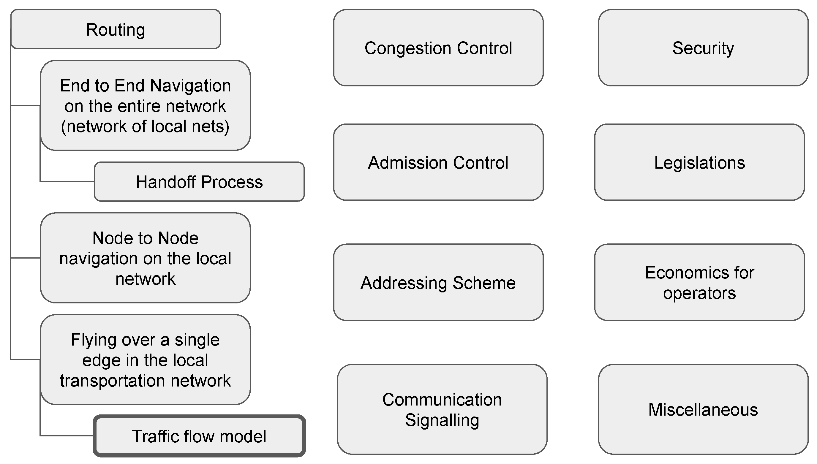
A common point of confusion is the relationship between the UTM concept and that of a traffic flow model. A traffic flow model is only a small aspect of IoD/UTM. In this paper, we are solely focused on the latter and Figure 1 helps situate this problem within the much larger context of IoD/UTM. Furthermore, in some contexts, UAS Traffic Flow Management (UTFM) is used to refer to UTM and this only aggravates the confusion over the term flow. Despite the similarity of the term flow, the traffic flow model is an entirely different concept than UTM or UTFM.
The motivation for creating a traffic flow model for UAVs is two-fold, as it relates to drone air traffic control architectures such as IoD:
- Firstly, it serves as a stable speed assignment scheme to be used for the movements of UAVs over the links in future UAV traffic control architectures such as IoD. Even though the speed assignment scheme is for UAVs on a single link (also known as Airways within IoD analogous to the roads for ground vehicles) as a first step, it is straightforward to generalize it to UAVs on a network (analogous to the road network for ground vehicles) in a future work as follows. For each drone, the single link is replaced by the path from the source to the destination for that drone. Then, to calculate the speed for the current drone we consider all the drones on that path as well as drones that are about to merge on that path in our speed assignment scheme.
- Secondly, we need computing tools for analyzing the behaviors of drones in the air and use the gained insights to improve the airway structures in UAV traffic control architectures (e.g., IoD) and provide additional capacity or services as the need for them becomes clear. Among these tools are traffic flow models. In the traffic literature for ground vehicles, traffic models have a long history and have been successfully used to analyze various traffic conditions such as formation of congestion and in general the interaction of vehicles with the road network infrastructure.
In this work, we are interested in microscopic traffic flow models. The traffic flow models can be divided into two main categories: Macroscopic and microscopic. In the former, we model the flow and the density at any location along the channel as if the vehicles form a gas traveling across a channel whereas in the latter, we model the individual position and the movement of the vehicles along the channel. Developing microscopic traffic flow modeling for UAVs is a new problem with its unique set of requirements. The closest related research area we can look for solutions is that of traffic flow models for ground vehicles. As we will see, even the limited existing works on UAV traffic flow models are adaptations of ground vehicle traffic flow models. A main characteristic of traffic flow models for ground vehicles is that they structure the road into one or multiple lanes and allow the movement of vehicles in this 2D space [10]. We call this general view of the modeling One/Multi-lane View (OMV). Within OMV, in the simpler case of one lane, no passing occurs. Most models are first introduced as one lane models and then with the aid of a separate lane-changing model are extended to multi-lane models [10,11,12].
An OMV-based model is limited in its application to UAVs as their movements are in the 3D space and lanes are not defined. Furthermore, not only the pass planning aspect is ambiguous in the 3D space, but also a low-level detail that adds to the complexity of a microscopic model and therefore should be aggregated. This is so since the overall goal is understanding the longitudinal movements of vehicles along the highway. Finally, in OMV models, a velocity will be assigned to each vehicle based on the congestion in their lane. In the same vein, it is ambiguous how the velocity must be determined in the 3D space with no lanes.
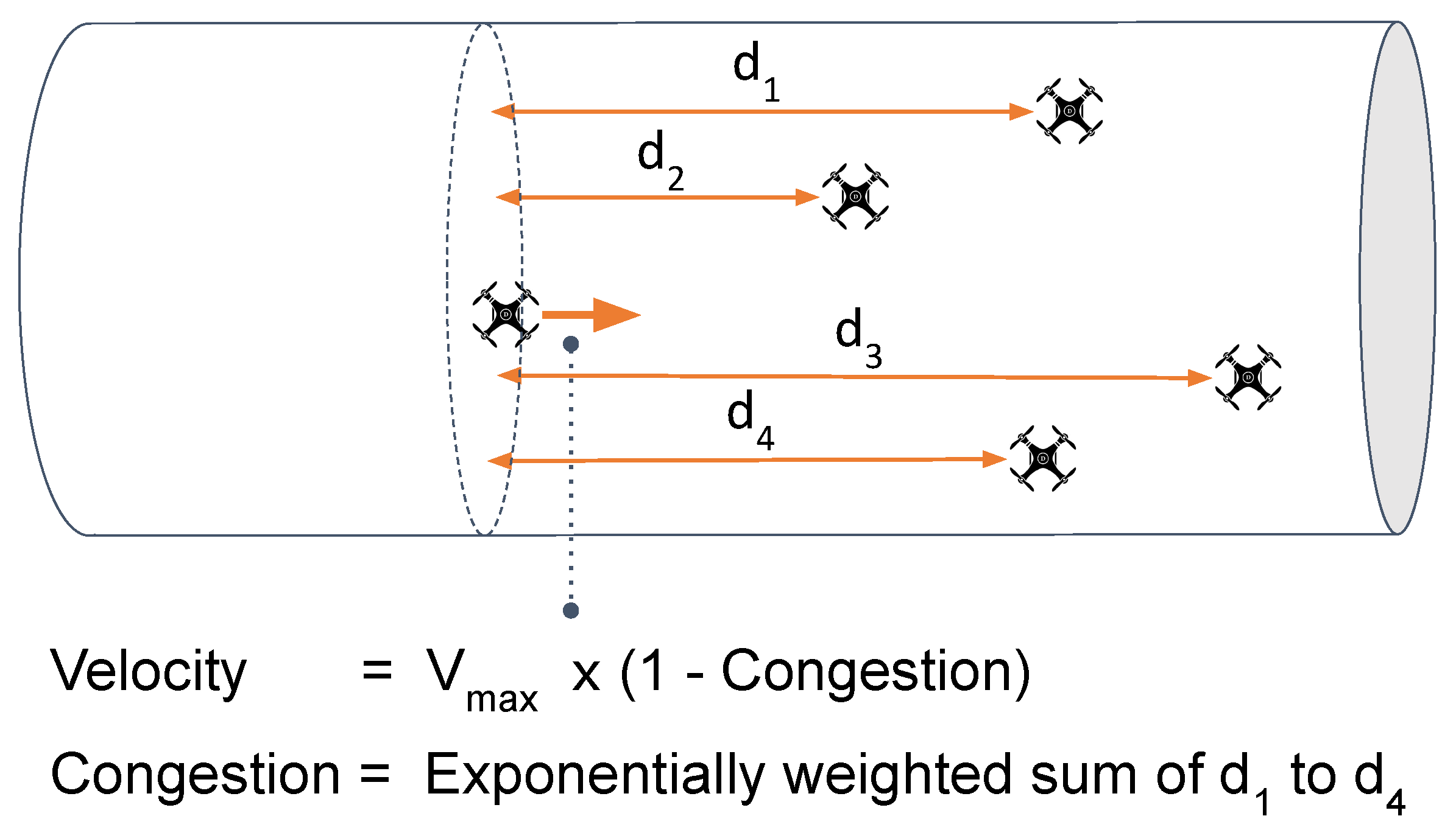
The main problem is to formulate a traffic flow model in a 3D space with no lanes for UAVs. We solve this problem by using a concept of a channel in which vehicles move and a density/capacity framework where for a vehicle to move forward, the density (or congestion) in its horizon must be under the set capacity of the channel. That is the velocity of each vehicle is set based on the perceived congestion (Figure 2). We call this general view in modeling, a DCV as an alternative to OMV. A DCV-based model also aggregates the pass planning aspect by allowing a vehicle to pass when the congestion is sufficiently low. Furthermore, if instead, we use an OMV model to represent the UAV traffic flow and velocity assignment, we effectively limit the movement of UAVs in an artificial way. This is because while ground vehicles can overtake each other only by moving to the adjacent lanes, we do not have the same channel topology for UAVs in the air. To illustrate the difference, even if we decide to organize the UAV traffic flow in lanes, one might envision many lanes and for a UAV to pass another one, any of these lanes can be used. In other words, any of the lanes are considered adjacent whereas on the road network this is impossible due to the 2D nature of the roads. Therefore, using an OMV model for UAVs will result in reduced traffic flow when used as a velocity assignment scheme.
In our model above, we have made the following simplifying assumptions for a futuristic world. Firstly, that all drones are aware of the location and the identity of the other drones. In fact, Federal Aviation Administration (FAA) requires almost all drones to be equipped with remote identification modules [13,14]. Secondly, every drone will be fully autonomous. Furthermore, we have assumed that drones can momentarily adjust their speed and also can assume zero velocity for a simplified model.
2. Related Works
Car following theories model the vehicles’ movements on a single lane as they follow each other [10]. There are separate lane changing models such as MOBIL (short for Minimizing Overall Braking Induced by Lane Change) [11] or the model in [12] that are used to extend these models to multilane.
Most (if not all) the modern microscopic models are modeled as either single lane or multilane. These include most of the well-known traffic flow models (and their extensions) such as Optimal Velocity Model (OVM) [15], Full Velocity Difference Model (FVDM) [10], Intelligent Driver Model (IDM) [16], and Newell’s Car-Following Model [17].
We argued in the introduction that pass planning should be aggregated. It is worth noting that in [18], for macroscopic models (with lanes), authors define a rate of lane changing based on macroscopic quantities such as density. In [19], based on the work of [18], authors combine this with a microscopic model together with quantizing the prescribed rate to make it applicable to the microscopic model. However, still, the model is essentially OMV-based, although to some extent the lane changing modeling complexity is avoided.
The implicit assumption we made was that with a low enough density of drones in any given space, the collision risk is negligible has a history in aviation as well. In the airspace, aircraft maintain a minimum required separation distance along at least one of the three dimensions, namely, along the route, vertical, and lateral. The required safe distances are put in place based on the field data as well as the economic cost of unnecessarily wide standards versus the cost of collision given the calculated upper bound on the risk of collision [20]. Similarly, in the work [21], from field data cited, the risk of collision was highly correlated with the density of the aircraft in an area. This notion was formalized using the gas model where the risk of collision between two aircraft in free flying paths is calculated and the mean collision-free distance is obtained. The goal will be to set the maximum permitted density in a way that keeps the mean collision-free distance above the desired threshold. In [22], expanded the gas model one step further by considering more advanced cases of collision such as overtaking model. According to [22], a uniform distribution over the flying direction will maximize the collision probability. Hence, the one-directional channel in our model avoids this pitfall. On the other hand, uniform distribution in space minimizes the probability of the collision.
2.1. UAV and Air Traffic Flow Models
To integrate UAVs in the airspace, researchers in NASA [23], proposed various structures for the airspace; including a road network like design (below the skyline; that is the tallest building height in a city) similar to our work in [1]. They set certain behavioral rules (i.e., a traffic flow model) for UAVs and accordingly extract the fundamental diagram of flow versus density. However, no stability analysis is done which is the standard in the traffic engineering community. Authors perform only a numerical simulation under acceleration from a standstill, followed by cruising and then braking of the leader on a flight lane. The traffic flow model is an OMV-based 1-lane model similar to that of ground vehicle models. In the model, authors consider the reaction delay. Their traffic flow model is based on a constant gain controller that adjusts the velocity to reach a goal velocity for some required separation. Additionally, the lane change is done collaboratively utilizing wireless communication between vehicles.
In [24], to study the wind effect on the fundamental diagram, the authors extend a car following model by Greenshields et al. [25] to include the wind force. This is a 1-lane model and no stability analysis is performed for the new model beyond what is already done for the original model by the research community.
In [26] the authors consider two self-organizing algorithms for UAVs. One is based on preferring a constant velocity for the agents, and in the other one, the preference is given to a fixed direction of flight. There is no channel in the air, instead, the flight happens in the open space, and the separation is enforced by considering the so-called “social” repulsion force between UAVs.
To formulate congestion, in [27], authors introduce the idea of pheromone deposits for the UAVs (similar to the ants), which act as repellents for other UAVs and can be considered as a metric for congestion. In [28], authors use the idea of fluid queuing models to also take into account the effect of weather disturbances on the congestion. The authors achieve this by adjusting the maximum flow rate (i.e., capacity) in the links (i.e., channels) in a stochastic way to simulate the weather disturbances effect.
Various macroscopic air traffic flow models exist for aircraft. In a pioneering work and inspired by the ground traffic flow models [29,30,31,32,33], Monen et al. develop a model called Cell Transmission Model. In this model, each cell is basically a one dimensional airway where aircraft flow enters from one end and leaves from the other end [34]. In [35], the authors extend the work in [34] by allowing flights in eight different directions, connecting the airspace volumes, rather that only one dimension that represents flights along jet routes and Victor airways. This is necessary to achieve a high fidelity model given the increasing number of flights that choose directions that are optimal given the wind direction. In [36], Sun et al. create a new model called large-capacity cell transmission model or CTM(L) for short where the word large refers to the fact that no hard limit on aircraft count is imposed on each cell within a sector other than the limit already imposed on the total aircraft count in the entire sector. A main advantage of this model is that by utilizing a multicommodity flow structure it resolves the issues related to the splitting and diffusion that was affecting the previous Eulerian models such as [32,33,34,35]. In [37], the authors improve over the work of [36] by reducing the number of states in the model by aggregating the number of aircraft on a edge on a given trajectory instead of looking at the count at the level of sectors. They also add ground and en-route delays to the model. In [38], the authors propose a supply-chain- based model which allows the delays to be accumulated by reducing the velocity of the aircraft rather than assigning zero velocity to the aircraft as is the case with the Cell Transmission Model.
There is a long history of using aircraft-level (microscopic) traffic flow models in aviation. One of the main uses for these models are detecting and resolving conflicts. However, due to the number of variables involved, the computational complexity of solving these models are much higher than the macroscopic models. In [39,40], the authors formulate a mixed integer linear programming (MILP) model that takes into account the capacity of the sectors and the airports and the goal is to minimize the air and ground delay cost for the flights. In the works that use a similar modeling framework based on mixed integer programming, the individual aircraft trajectories in the space are discretized. So in this sense, they are similar to the discrete microscopic traffic flow models (such as the cellular automata based models). In [41], the authors discretize the trajectory of the flights by segmentation of the trajectory and propose a MILP model for the traffic flow. In [42], Grabbe et al. convert the flight scheduling problem into an instance of the job shop scheduling problem. The authors then formulate this problem as a MILP instance which is then solved using the CPLEX software. In [43], the authors solve the traffic scheduling problem by picking a critical collection of the flights and sectors and giving them a higher priority while the solution to the other flights and sectors is formed around the solution to this collection. This model is based on [39] and the speedup is achieved by reducing the problem space by the careful selection of the critical collection. In [44], the authors give an architecture to solve the latter model using parallel processes for a faster computation time. In [45], Bayen et al. give a linear programming model that minimizes the arrival time for each aircraft modeled while maintaining a separation gap between the aircraft.
2.2. Ground Vehicle Traffic Flow Models
Traffic flow theory finds its root in the work of Greenshields in 1930s [25]. Traffic flow models can be classified across different dimensions, such as the aggregation level. Macroscopic models take a high-level view of traffic flow similar to the flow of liquids or gases. Quantities of interest are local density, flow, mean speed and variance and their evolution through time [29,30,46,47,48,49,50]. Microscopic models (e.g., see below) to which our models belong such as car-following or cellular automata models describe the interaction of each driver with its environment. In these models, we are interested in quantities such as individual position and speed and perhaps acceleration [46].
Within microscopic models, we categorize the models based on their relevance to our model. In particular, a distinction is made between 1-lane or multi-lane models. Many of the classic models are 1-lane models. Among the classics are the Optimal Velocity Model (OVM) [15], Full Velocity Difference Model (FVDM) [10], and Intelligent Driver Model (IDM) [16] whereas [51] is a more recent example. However, it is possible to extend these to multi-lane models by use of a lane change model such as MOBIL which dictates the rule of when it is safe and beneficial for a vehicle to change lanes [11].
Another distinction is whether a vehicle takes the optimal velocity in equilibrium instantly similar to our model or gradually. Models with delays can demonstrate delay-induced traffic phenomena at the expense of added complexity. No delay classic models include Reuschel and Pipe’s models [52,53]. Classic models such as OVM [15], FVDM [10], and Newell’s Car-Following Model [17] exhibit delay. In [54], the authors extend FVDM by anticipating the behavior of the next vehicle in the front and hence reducing the delay in the reaction.
Furthermore, one difference is whether the drivers only react to the immediate vehicle in the front or beyond. In particular, in multi-vehicle anticipation models, a few vehicles at the front are considered by the driver for better stability (fewer accidents) [46]. In [55], the authors extend some of the traffic flow models including OVM, FVDM, and IDM by adding multi-vehicle anticipation features. In [56,57], the authors extend OVM and Gipps [58].
Additionally, a distinguishing factor is whether the velocity is adjusted based on the time gaps between two vehicles or the space gaps (such as our model). Models such as FVDM [10,16] use time gaps whereas OVM [15] and Newell’s car following model [17] use space gaps.
We know of very few models that can be solved analytically. A 1-lane model by Hasebe et al. [59] uses the tangent hyperbolic function to relate the distance between only subsequent vehicles to their velocity with an exact solution for various delays.
An interesting class of car-following models are those based on the cellular automata. In these models, both the time and the space are discretized into time steps and cells. In [60], the authors propose a model where the cells’ width can vary. This helps represents the obstacles in the road and the narrowness of the lanes. In [61], the authors study the effect of in-flow and random deceleration on the average traffic velocity, using a single lane cellular automata model. In [62], the authors train a neural network based lane-changing model according to the vehicle overtaking trajectories in a simulator.
In a highly related work [63], Newell designs a 1-lane model that can be solved analytically. It was later extended by Whitham [64], finding various exact wave solutions, such as periodic and solitary waves. The model assigns the velocity at time to a follower vehicle according to an exponential decay congestion term at time t where is a delay constant. The congestion term is based on only the distance between the follower and the leader. This results in a non-linear differential equation which Newell transforms into a linear form when and cars are identical. There are similarities and differences in how this model relates to our work. We use a similar technique to make our differential equations linear. Additionally, we use an exponential decay scheme, but our formulation is different in that we use all the vehicles in the front and not just the first one. Our model is DCV-based and can exhibit passing or blocking behavior according to the set value for capacity whereas this is a 1-lane model. Furthermore, except for having the same horizon for each car, we do not require cars to be identical. Certain details of the models are also different. For example, our model being DCV based does not have a concept of minimum headway or vehicle length.
3. Model and Analytical Solution
In this section, we present our microscopic lane-free traffic flow model in detail. Furthermore, we present the model’s closed-form and piece-wise closed-form solutions for blocking and passing regimes, respectively. Finally, we determine if the proposed closed-form solution is suitable for performing stability analysis.
In our model, we consider a sequence of vehicles numbered as 0 up to from the first to the last vehicle traveling along an infinite link. The position of each vehicle is designated by for some chosen origin (Figure 3).
The vehicles adjust their speeds based on the distances to the vehicles in front of them according to some exponential weighting scheme. This model is represented by the non-linear differential equations described by (1)–(3) as follows.
where the constant is the maximum free flow speed for vehicle i and is the congestion factor. The constant is called the horizon in front of each vehicle. Once the leading cars are inside this horizon, they will have a substantial effect on slowing down vehicle i, otherwise their effects will be small. Parameter is called capacity. Intuitively, is roughly the maximum number of vehicles permitted inside the horizon . One way to see this is that if all vehicles in front of a vehicle i are located right in front of it, it takes vehicles for to be 1 in (2) and as a result vehicle i to slow down to 0 velocity (i.e., a perfect jam). However, it is worth mentioning that need not be an integer and can take any real positive value.
Following this, in Section 4.2, we prove that given , faster vehicles cannot overtake slower vehicles, corresponding to effectively a 1-lane link (since intuitively only 1 vehicle is allowed in ith vehicle’s horizon as explained above). However, if , faster vehicles might be able to pass slower vehicles if certain conditions are satisfied; corresponding to a multi-lane link. We refer to these two different regimes as passing and blocking hereafter.
3.1. Discussion and Design Philosophy
In this section, we discuss the model in greater depth as well as some of the details of the model. Some of the main design decisions or features of the model are already presented in the introduction and throughout the chapter and we do not revisit them here.
Originally, in our architecture, Internet of Drones (IoD) [1], we proposed each airway to be a single lane to reduce the technological burden on drones to safely execute a passing maneuver. However, it is plausible that as the technology matures, allowing passing will increase the efficiency of airway usage. We are interested in both of these cases in this chapter.
We argued earlier that the pass planning should be aggregated. In pass planning, we are dealing with specific maneuvers that happen for a vehicle to change its lateral position (in DCV models) or lane (in OMV models) which has low relevance to the goal of studying the longitudinal movements. Furthermore, from a technical perspective, passing maneuvers for UAVs are less structured and require a more complex passing model.
One difference between ground vehicles and autonomous UAVs is the delay aspect. We have assumed the delay for an autonomous vehicle to adjust its velocity according to the traffic condition is negligible. This is not an entirely correct assumption as while it is plausible to assume the perception and reaction time will be very small compared to the human-operated vehicles, still, there will be a delay component dictated by the mechanical properties of the system and its inertia.
Another design choice that we made was the use of space gaps between vehicles compared to the time gaps. Time gaps seem to be the reasonable choices in cases where there is a high disparity between the maximum velocities of different vehicles. However, they also lack a crucial component for use for the airway. Since it is expected that the airway links will be very low altitude, they will be affected by the wind disturbances present in the urban centers. These can displace a UAV by several meters. Therefore, it seems the safest choice is to space vehicles apart enough to safeguard for these disturbances. While time gaps are important as well, we cannot rely solely on them to ensure the safety of flights.
A difference between our model and multi-anticipation models as reviewed in Chapter 1 is how the congestion is calculated. In our model in accordance with DCV, we take into account all the vehicles at the front whereas in multi-anticipation models, given the OMV frameworks, only the vehicles on the same lane are considered.
Our model makes it easy to introduce stationary or moving bottlenecks without modifying the model. For example, in the DCV framework, we can adjust the capacity locally by adding dummy vehicles (stationary or moving) whereas in the OMV case, we need to deal with explicit lane closures.
We study the passing and blocking regimes separately below.
3.2. Blocking Regime
We use a differential equation technique to transform the characterizing differential equation, i.e., (1) into a linear differential equation. A similar technique was used in [63]. Defining the auxiliary variable
we will have
After simplifications, we will have
Equation (7) creates a set of homogeneous linear differential equations. There is no shortage of ways to solve this set of equations. One particular way which is especially applicable here is to solve a series of first-order linear differential equations as follows. First, let us define
Starting from , it can be solved by solving the following differential equation
Since is a known function in time, can be solved easily by the standard methods as it is a first order linear differential equation. As a result, now is a known function in time, and similarly can be solved. Applying this method recursively, the whole set of equations can be solved by solving the resulting first order linear equation for each .
By solving the set of equations using a method like above, in the simple case where all ’s are unique, the general solution to this set of differential equations can be written as
where will be determined using the initial conditions.
In the case where velocities are not unique, the solution looks a bit more involved but can be expressed in the following way. First, let U be the set of smallest indices of vehicles with unique maximum velocities. Let be the multiplicity of each velocity for vehicles 0 to i (that is those ahead of vehicle i). Then the solution for will be of form
and will be determined by the initial conditions.
3.3. Passing Regime
The same analytical approach of the blocking regime applies to the passing regime. However, after each overtake, we need to solve the differential equations again for the vehicles involved in passing and all the vehicles behind them. Therefore, we need to compute the passing times or in other words the roots to the equations of type
or equivalently
The problem is to find the equation that has the smallest passing time and the passing time itself. This is necessary, so the coefficients in the solution can be corrected as soon as a passing occurs.
We have not developed any heuristics for the root-finding algorithm, but it seems plausible that an algorithm can generate a shortlist of candidate equations that are suspected to have the smallest root based on various heuristics such as the distance between two vehicles and the velocity differences among other things. It is then easy to verify whether the obtained passing time is indeed minimal by checking that only one pass has occurred.
3.4. Stability Analysis
As mentioned, a differential equation technique was used to turn (5) and (6) into the linear form of (7). However, since the variables in terms of which (7) is linear are at their cores exponential functions, they can never be 0. This is relevant since the point where all state variables are 0 is the unique equilibrium point for the linear systems of the form
where
Putting (7) in this matrix format will yield a lower triangular matrix A whose diagonal elements are and therefore non-zero. Since in a lower triangular matrix, the eigenvalues are the diagonal elements and no 0 eigenvalue exists in this case, the determinant is non-zero. Therefore, we cannot use our analytical result for stability analysis. In the next section, we rely on linearization and numerical simulation to study the stability of the model in the blocking regime.
4. Model’s Properties
This section presents some of the properties that are expected from a sound model. We show our model does not result in a negative velocity for any of the vehicles. Furthermore, we show that the vehicles with smaller maximum velocities will not pass vehicles with larger maximum velocity. Lastly, we analyze the system’s passing and blocking behavior and state the conditions that enable the vehicles to pass one another.
4.1. Soundness
In this section, we prove a few theorems that establish some of the expectations we have from a sound model.
We expect the velocities that are prescribed for each vehicle to be in the direction of the flow; that is non-negative. Here we show that our model never prescribes a negative velocity.
Theorem 1 (Non-negative velocity).
Given vehicle i with maximum velocity in a platoon, .
Proof.
For the sake of contradiction, and without loss of generality, let n be the vehicle closest to the front in a platoon whose velocity will become negative. Call the moment when the velocity becomes zero, . Taking a time derivative from both sides in (1), we will have
Evaluating (16) at , we will get
where the strict inequality holds since no vehicle j with can have a negative velocity due to our assumption and at least the first vehicle has a positive velocity. Since the derivative of velocity is positive, the velocity cannot become negative. □
Next, we prove that a vehicle with a smaller maximum velocity cannot pass a vehicle with a larger maximum velocity. One might perceive this is possible if the faster vehicle is subject to more congestion, but we show this will never be the case.
Before presenting the next theorem, let us first define a platoon. A platoon refers to a group of vehicles that travel together while keeping their distances under some upper bound (i.e., the distance of the first to the last vehicle is always bounded by some constant).
Theorem 2 (No overtaking by slow).
Given vehicles i and in a platoon, if
and
then
for all .
4.2. Passing or Blocking Behavior
First, we prove a necessary and sufficient condition for a vehicle to pass another. Then we prove one of our main results that there exists a threshold for above which, the model permits passing and below which it is not permitted. This constitutes a regime change in our model.
Theorem 3 (Passing condition).
Given vehicles i and in a platoon with
and
vehicle will pass vehicle i if and only if at the time of passing the following condition is met
Proof.
Equation (2) and Theorem 1 imply that
We use (1) for vehicle i and (22) for vehicle (which also holds here) in the following. Vehicle will pass vehicle i if and only if we have (at time of passing)
□
The next corollary states one of our main results.
Corollary 1.
is a sufficient condition for no passing to occur.
5. Asymptotic Behavior Analysis
In this section, we analyze the system’s asymptotic behavior in passing and blocking regimes. More precisely, we show that in the passing regime, the order of vehicles in the system remains stable (i.e., does not change) in an effort to prove stability-like properties for the model, given that the problem, in this case, does not lend itself well to a typical stability analysis around some well-defined equilibrium point. In addition, we present a condition that leads vehicles to be sorted through their passing based on their maximum velocities as time approaches infinity. In the case of the blocking regime, we perform both linear and non-linear stability analyses. For the former, we show an equilibrium point exists in which all vehicles travel in the infinite road with the same velocities. Furthermore, we prove the asymptotic linear stability and local stability of the scalar capacity model. For the latter, we consider vehicles located on a ring and show numerical evidence that an equilibrium point for the velocities exists.
5.1. Passing Regime
We cannot perform a straightforward stability analysis in the passing regime since it is not clear how to conceptualize a reasonable equilibrium point in this case. However, the following theorems will be useful in understanding the passing regime in the asymptotic case.
Theorem 4 (Order stability).
There exists a time T after which the order of vehicles in the system will not change.
Proof.
The number of possible orderings is fixed. Additionally, a slower vehicle cannot pass a faster vehicle according to Theorem 2. This creates a partial order on the set of ordering configurations. Therefore, at any state, either the system remains in that state forever or will move to a new state according to the partial order with no going back. Since the number of new admissible states is finite, the system will have to stay in one of the states forever after some time T. □
One might suspect that given enough time, vehicles will be sorted based on their maximum velocities; that is the fastest vehicle will become the first vehicle, the second fastest vehicle will be the second, and so on. However, as we will see in Theorem 5, this will not necessarily be the case unless there is a meaningful difference between the velocities of any two vehicles. Intuitively, this can be understood in the following way; if a highway is congested to some extent and two vehicles have slightly different maximum velocities, it is difficult for the fast vehicle to gain enough speed difference to take advantage of the little space available and overtake the slow vehicle.
Theorem 5 (All fast vehicles pass condition).
For an arbitrary set of N vehicles with the maximum velocities and arbitrary initial ordering, as time goes to infinity, vehicles will be sorted via passing according to their maximum velocities, if and only if the following holds
Proof.
We first prove given the condition in (32), a sorted order will be achieved. From Theorem 4, the final order will be stable. We take the moment we reach the stable state as the origin of time. For the sake of contradiction, assume the stable order is not sorted according to the maximum velocities. Let be the first vehicle with a larger maximum velocity than vehicle i, that is
Since the vehicles in front of i are faster than i, as the time goes to infinity, we have
So for any sufficiently small , there exists some such that for
we have
For any time , we can rewrite (1) for vehicle as
For vehicle i, we have
To prove the passing occurs, it is sufficient to show
for all and some fixed . Equation (32) implies that
for some . Replacing (40) in (37), yields
where the last inequality holds for any where is sufficiently small. Therefore will pass i which will be a contradiction. Therefore, the order is only stable, if it is sorted according to the maximum velocities.
Now, let us assume the set of given maximum velocities are sorted by index so that a larger index corresponds to a larger maximum velocity. To prove the other direction of the theorem, we assume the reverse of (32) holds
where without loss of generality, we assume and are the two velocities that maximize the middle term. The equality above can be inspected to be true by dividing both the numerator and the denominator in the second term by and observing that only consecutive indexes can result in a maximum.
We construct a non-passing example as follows. Vehicles and j will have maximum velocities and . All faster vehicles than will be placed in front of the th vehicle. Furthermore, all slower vehicles than will be placed behind the jth vehicle. This might induce a change of indices which will be done as needed.
For the sake of contradiction, let us assume the jth vehicle will pass the th vehicle. At the time of passing, Theorem 3 implies
given that from (2) and Theorem 1 we have
which results in a contradiction. □
5.2. Blocking Regime: The Case of Linear Stability Analysis
The standard tool to study the asymptotic behavior in this case is stability analysis. We will study linear stability analysis for vehicles placed on an infinitely long road.
5.2.1. Equilibrium Point for the Infinite Road Case
Our state variables are the velocities of each vehicle excluding the first vehicle which has a constant velocity of . Assuming we have a sequence of N vehicles such that
for all
there exists an equilibrium point where all vehicles travel at the same velocity
5.2.2. Local (Platoon) and Linear Stability Analysis
Theorem 6.
In the blocking regime, given a platoon of N vehicles, the Scalar Capacity Model has both local (platoon) and asymptotic linear stability.
Proof.
We first prove the asymptotic linear stability of the model and then the local (platoon) stability will follow as a special case. Our state variables are the velocities of all vehicles except the leader as it is fixed. Without loss of generality, we assume
for all (otherwise, we do not have a single platoon according to Lemma A2 in the Appendix A). We define the gap in front of vehicle i and the gap between vehicle n and i, respectively, as
In the equilibrium we have
Now we apply a small perturbation to the velocity of each follower as follows
For ’s we define an identity similar to (50) as follows
Assuming we kick all the follower vehicles out of equilibrium, for the nth vehicle we will have
After linearization and simplification using (51), we get
By inspection, A is a lower triangular matrix with only negative elements. Since the eigenvalues of a lower triangular matrix are the elements of the diagonal, all the eigenvalues of the matrix are negative. Therefore, according to the linear stability theory, variables are stable with an equilibrium point of all 0s. Hence, a similar thing can be said about . To understand the rate of convergence, we calculate the eigenvalues which are the elements of the diagonal of A. In other words, the eigenvalues are the coefficients of in (58). By inspection, we have
where the last equality is due to (51) and knowing . Therefore, the bigger the difference between and , the faster the convergence will be to the equilibrium point. The above proved the asymptotic linear stability of the model. Linear (platoon) stability is proven by considering the special case where there is 0 initial perturbation to the position and velocity of vehicles
and accordingly
□
5.3. Blocking Regime: The Case of Nonlinear Stability Analysis
In this section, we perform the non-linear stability analysis for vehicles placed on a ring road. Note that (2) and (3) are adjusted accordingly to become symmetrical for any vehicle i (i.e., now each vehicle regardless of their numbering is a follower to every other vehicle on the ring road).
5.3.1. Equilibrium Point for the Ring Road
Given a fleet of identical vehicles with maximum velocity traveling on a ring road, the exact locations of each vehicle are not important to us. However, their relative distance is important. We take the set of velocities as our state variables. Since the motion equations for all vehicles are symmetrical on the ring road, an immediately obvious equilibrium point is the case where all velocities are identical. This is equivalent to saying that all gaps are identical; that is
where L is the circumference of the ring road and N is the number of vehicles. We define the overall density as
The equilibrium velocity is calculated as follows:
Using the identity for the sum of the geometric series, we obtain
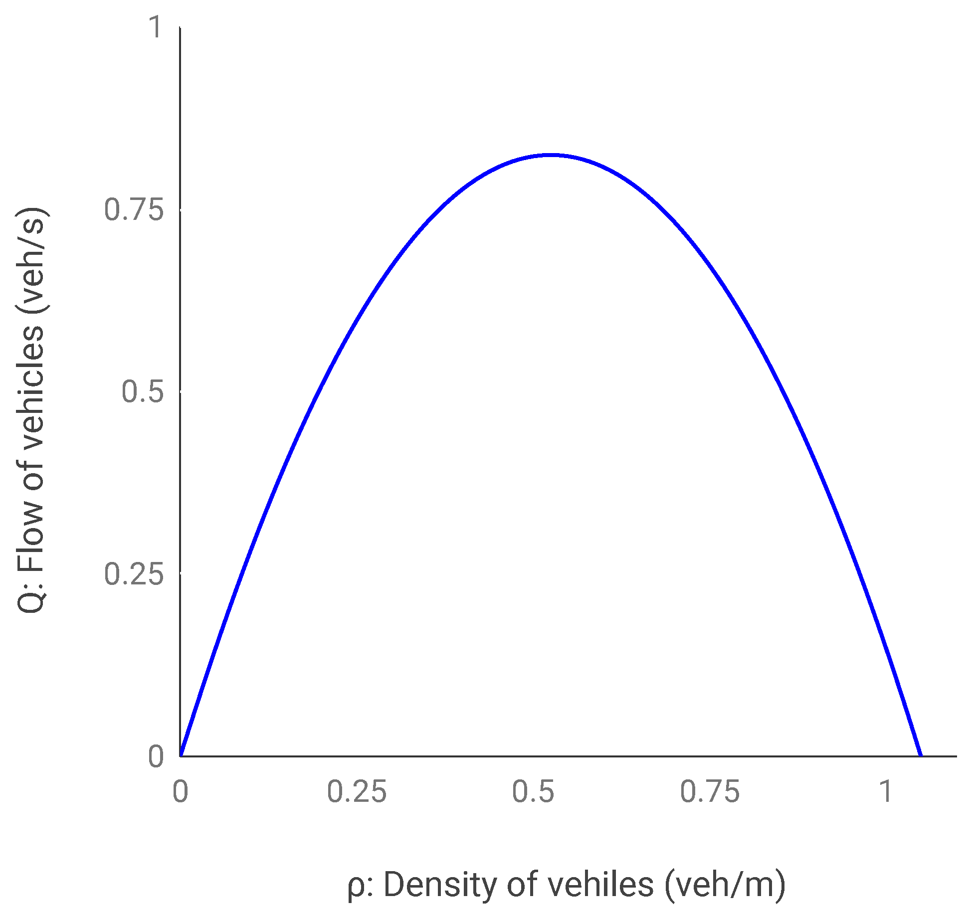
Vehicle flow, velocity, and density are related by
which results in the diagram in Figure 6 relating the traffic flow Q to the density . This graph is also one of the fundamental diagrams of a traffic flow model and it gives insight into the macroscopic behavior of our microscopic model. It also gives an intuitive justification for the soundness of our model, since all traffic flow models (including those cited in this work) produce a more or less similar graph. That is the traffic flow increases as the density increases till we reach a peak capacity after which adding any more vehicles will only serve to decrease the flow.
5.3.2. Numerical Experiments
In this section, we initiated the system with a variety of conditions and observed whether the system approached the equilibrium point. We used a chosen background density composed with a smaller region of higher density. We observed how this irregularity affected the system’s stability. Our experiments parameters were chosen as follows:
- L = 1000 m, length of the ring road (m).
- = 10 m, length of the horizon in front of each vehicle.
- = 6 m/s, for all vehicles.
- = 10, model’s capacity.
- = 0 s, = 500 s, start and finish time of simulation.
- , global density of vehicles. In other words, we have 500 vehicles on the ring road (a minimum number of vehicles that is required for a realistic simulation [46]). Note that this does not necessarily translate into an unreasonably high density of vehicles since the vehicles are not directly behind each other in the 3D space. In other words, they can be placed anywhere on the vertical plane that belongs to them.
To produce Figure 7 and Figure 8 we distributed the vehicles in two regions. One region consisted of 30% of the ring road and had the highest possible uniform density of the vehicles and the remaining vehicles were distributed in the rest of the ring road evenly; so as to make the overall density as above. These experiments provided evidence that no matter how far from equilibrium the system was, it converged to the equilibrium. Additionally, we performed the same test with the same number of vehicles when 10% or 20% of the ring road had a maximal traffic jam and each case produced essentially the same graphs.
6. Discussion and Future Work
Our work leaves many open questions. An important question is whether it is possible to add some mechanism for the delay, without losing the closed-form analytical solution feature of the model. It is an interesting avenue for research to analyze how delay modifies the stability analysis and introduces some critical traffic flow phenomena such as hysteresis in traffic flow and stop-and-go waves.
Another avenue for research is adding some dummy vehicles to play the role of moving or stationary obstacles for the traffic flow. This works by consuming the capacity of the airway/road dynamically. It organically gives rise to the inclusion of obstacles without modifying the model. In the same vein, it is possible to add weights to the exponential congestion term for different vehicles or dummy vehicles (obstacles). Currently, in our model, all these weights are equal. The ability to set weights can give us powerful tools for tuning the strength of these obstacles.
In terms of integration with an air traffic control architecture for drones (such as IoD), the following three points are pertinent.
- Given a scheduler that schedules the arrival times at certain points of interest (call them nodes), our work in this paper is related to UAVs flying through the links in a way that is stable and respects the link capacity. We need both these systems to work in tandem. That is the scheduler sets the target arrival time windows for each node for a UAV and the role of the traffic flow model is to meet those targets. The main inputs to the traffic flow model are the maximum velocity constants for each UAV. Therefore an important missing piece is a module that takes the scheduled times and translates them to appropriate values of maximum velocity constants periodically.
- An issue that needs to be addressed concerning work in this paper is that the speed of each drone is momentarily adjusted to the current state of traffic on the link. This is especially troublesome when a UAV enters a new link. While the congestion in the previous link might have been low and thus the UAV has been flying at high speed, suddenly it might face a high level of congestion and must reduce its speed sharply which might be physically impossible. Therefore mechanisms must be put in the place to smooth the transition between the links.
- Another use for our work in this paper in the context of IoD is traffic engineering of the airways capacities. Within the realm of any traffic control architectures (such as IoD), the traffic flow model might fail to meet the targets set by the scheduler, due to some links being persistently overloaded. It will be of great utility to design an algorithm that processes the data about airways utilization rate and the success rate in meeting the arrival targets and translate them into decisions about adjusting the capacity of the airways.
Furthermore, it is an interesting avenue for research to show more stability properties hold for our traffic flow model. In particular, the string stability analysis will add to the richness of the current work. Additionally, it would be an important problem to consider wind fluctuations along the channels. In other words, the airflow might be different throughout the channel and these disturbances will need to be considered for a richer model.
Another important problem to consider is in case of applying our model to a specific airspace geometry with known dimensions, what values should we assign to the parameters in our model such as the capacity for the channel, given the analysis similar to that of [20,21,22] to minimize the risk of collision. Furthermore, given any set channel capacity, it would be interesting to calculate the collision rate.
Finally, the grand contribution would be to use the real life drones to validate an enhanced version of our model with delay.
7. Conclusions
In this paper, we introduced a microscopic traffic flow model that can be used to study traffic patterns of unmanned aerial vehicles in the air as they become ubiquitous in the future. The model is equally applicable to the study of the traffic flow of ground vehicles on the road. We advanced the state of art by introducing a scalar capacity parameter for the airway (or roads) rather than the traditional approach of modeling links as 1 lane or multi-lane. This is suited for the study of the 3D nature of UAV flights as opposed to the 2D nature of ground vehicles movements while also resulting in a simpler model for ground vehicles by abstracting away the pass planning aspect. By adjusting the scalar capacity parameter, the model can exhibit passing or blocking behaviors. In the former, vehicles are free to pass each other while in the latter, no vehicle can pass another one similar to a one-lane road. Our model can be solved analytically for the blocking regime and piece-wise analytically in the passing regime. For the blocking regime, we proved linear local (platoon) stability as well as asymptotic linear stability. Additionally, using numerical simulation, we showed evidence for non-linear stability. For the passing regime, we proved theorems outlining the asymptotic behavior of the model such as whether every faster vehicle gets a chance to pass slower vehicles as time goes to infinity and what the final order of vehicles will be after all the overtakings are completed. Lastly, we proved a main theorem characterizing the transition from blocking to passing as we adjust the scalar capacity parameter.
Author Contributions
Conceptualization, M.G.; methodology, M.G.; software, M.G.; validation, M.G., R.B., S.L.W., and Z.G.; formal analysis, M.G.; investigation, M.G., R.B., S.L.W., and Z.G.; resources, M.G. and Z.G.; data curation, M.G.; writing—original draft preparation, M.G., R.B., S.L.W., and Z.G.; writing—review and editing, M.G., R.B., S.L.W., and Z.G.; visualization, M.G., Z.G.; supervision, R.B., S.L.W.; project administration, R.B., S.L.W.; funding acquisition, R.B., S.L.W. All authors have read and agreed to the published version of the manuscript.
Funding
This research received no external funding.
Institutional Review Board Statement
Not applicable.
Informed Consent Statement
Not applicable.
Data Availability Statement
Not applicable.
Acknowledgments
We would like to thank Claudio Cañizares, Ehsan Nasr Azadani, and Amir Khajepour for fruitful discussions on the subject.
Conflicts of Interest
The authors declare no conflict of interest.
Appendix A. Helpful Lemmas
Lemma A1 (Passing threshold).
Given only two vehicles on the road with
given enough time, vehicle 1 will pass vehicle 0 if and only if
Proof.
Proving vehicle 1 passes vehicle 0 implies
is a straightforward consequence of Theorem 3 since
at all times including the passing time between vehicles 0 and vehicle 1.
In the other direction, we prove
implies for all times, that
We first prove the two vehicles will meet as a condition for Theorem 3, so we can apply that theorem.
Variable takes its minimum value when vehicle 0 and 1 are (hypothetically) in the same position, that is . Therefore, a pass will occur in that case since we will have
and can use Theorem 3,
Therefore, at all other times,
This implies that there exists a time when the two vehicles will meet, or in other words they are in the same position
Therefore, according to Theorem 3, vehicle 1 will pass vehicle 0. □
Without loss of generality, assume vehicle n is the first vehicle for which
In the following lemma, we show if a vehicle n in a sequence of vehicles following a leader with speed has a maximum speed
then this will result in the creation of two platoons. When
this is easy to see. However, when the maximum speeds are equal, one can see that this still holds. More formally:
Lemma A2 (Platoon splitting).
Given a platoon of n vehicles with stable orders with an extra vehicle n with
and where vehicle 0 to are in equilibrium, if
for
then vehicle n is not part of the platoon.
References
- Gharibi, M.; Boutaba, R.; Waslander, S.L. Internet of drones. IEEE Access 2016, 4, 1148–1162. [Google Scholar] [CrossRef]
- Gharibi, M. On the Integration of Unmanned Aerial Vehicles into Public Airspace. 2020. Available online: https://uwspace.uwaterloo.ca/handle/10012/15943 (accessed on 11 September 2021).
- NASA. NASA UTM 2015: The Next Era of Aviation. Available online: http://utm.arc.nasa.gov/utm2015.shtml (accessed on 11 September 2021).
- NASA. UTM: Air Traffic Management for Low-Altitude Drones. Available online: https://www.nasa.gov/sites/default/files/atoms/files/utm-factsheet-11-05-15.pdf (accessed on 11 September 2021).
- Kopardekar, P. Safely Enabling UAS Operations in Low-Altitude Airspace. Available online: https://ntrs.nasa.gov/api/citations/20150006814/downloads/20150006814.pdf (accessed on 11 September 2021).
- Amazon.com Inc. Determining Safe Access with a Best-Equipped, Best-Served Model for Small Unmanned Aircraft Systems. Available online: https://www.nasa.gov/sites/default/files/atoms/files/amazon_determining_safe_access_with_a_best-equipped_best-served_model_for_suas2_0.pdf (accessed on 11 September 2021).
- Amazon.com Inc. Revising the Airspace Model for the Safe Integration of Small Unmanned Aircraft Systems. Available online: https://www.nasa.gov/sites/default/files/atoms/files/amazon_revising_the_airspace_model_for_the_safe_integration_of_suas6_0.pdf (accessed on 11 September 2021).
- Google Inc. Google UAS Airspace System Overview. Available online: https://www.nasa.gov/sites/default/files/atoms/files/googleuasairspacesystemoverview5pager-508_0.pdf (accessed on 11 September 2021).
- NASA. NASA UTM. Available online: https://www.nasa.gov/ames/utm (accessed on 11 September 2021).
- Jiang, R.; Wu, Q.; Zhu, Z. Full velocity difference model for a car-following theory. Phys. Rev. E 2001, 64, 017101. [Google Scholar] [CrossRef] [PubMed] [Green Version]
- Kesting, A.; Treiber, M.; Helbing, D. General lane-changing model MOBIL for car-following models. Transp. Res. Rec. 2007, 1999, 86–94. [Google Scholar] [CrossRef] [Green Version]
- Toledo, T.; Koutsopoulos, H.N.; Ben-Akiva, M.E. Modeling integrated lane-changing behavior. Transp. Res. Rec. 2003, 1857, 30–38. [Google Scholar] [CrossRef] [Green Version]
- FAA. Remote Identification for Drone Pilots. Available online: https://www.faa.gov/uas/getting_started/remote_id/drone_pilots/ (accessed on 11 September 2021).
- ASTM International. Standard Specification for Remote ID and Tracking. Available online: https://www.astm.org/Standards/F3411.htm (accessed on 11 September 2021).
- Bando, M.; Hasebe, K.; Nakayama, A.; Shibata, A.; Sugiyama, Y. Dynamical model of traffic congestion and numerical simulation. Phys. Rev. E 1995, 51, 1035. [Google Scholar] [CrossRef]
- Treiber, M.; Hennecke, A.; Helbing, D. Congested traffic states in empirical observations and microscopic simulations. Phys. Rev. E 2000, 62, 1805. [Google Scholar] [CrossRef] [Green Version]
- Newell, G.F. A simplified car-following theory: A lower order model. Transp. Res. Part B Methodol. 2002, 36, 195–205. [Google Scholar] [CrossRef]
- Laval, J.A.; Daganzo, C.F. Lane-changing in traffic streams. Transp. Res. Part B Methodol. 2006, 40, 251–264. [Google Scholar] [CrossRef]
- Laval, J.A.; Leclercq, L. Microscopic modeling of the relaxation phenomenon using a macroscopic lane-changing model. Transp. Res. Part B Methodol. 2008, 42, 511–522. [Google Scholar] [CrossRef]
- Reich, P.G. Analysis of long-range air traffic systems: Separation standards—I. J. Navig. 1966, 19, 88–98. [Google Scholar] [CrossRef]
- Alexander, B. Aircraft density and midair collision. Proc. IEEE 1970, 58, 377–381. [Google Scholar] [CrossRef]
- Endoh, S. Aircraft Collision Models. Ph.D. Thesis, Massachusetts Institute of Technology, Cambridge, MA, USA, 1982. [Google Scholar]
- Jang, D.S.; Ippolito, C.A.; Sankararaman, S.; Stepanyan, V. Concepts of airspace structures and system analysis for uas traffic flows for urban areas. In AIAA Information Systems-AIAA Infotech@ Aerospace; American Institute of Aeronautics and Astronautics: Reston, VA, USA, 2017; p. 0449. [Google Scholar]
- Battista, A.; Ni, D. Modeling Small Unmanned Aircraft System Traffic Flow Under External Force. Transp. Res. Rec. 2017, 2626, 74–84. [Google Scholar] [CrossRef]
- Greenshields, B.; Channing, W.; Miller, H.; Bibbins, J.R. A study of traffic capacity. In Highway Research Board Proceedings; National Research Council (USA), Highway Research Board: Rockville, MD, USA, 1935; Volume 1935. [Google Scholar]
- Virágh, C.; Nagy, M.; Gershenson, C.; Vásárhelyi, G. Self-organized UAV traffic in realistic environments. In Proceedings of the 2016 IEEE/RSJ International Conference on Intelligent Robots and Systems (IROS), Daejeon, Korea, 9–14 October2016; pp. 1645–1652. [Google Scholar] [CrossRef] [Green Version]
- Samir Labib, N.; Danoy, G.; Musial, J.; Brust, M.R.; Bouvry, P. Internet of unmanned aerial vehicles—A multilayer low-altitude airspace model for distributed UAV traffic management. Sensors 2019, 19, 4779. [Google Scholar] [CrossRef] [PubMed] [Green Version]
- Zhou, J.; Jin, L.; Wang, X.; Sun, D. Resilient uav traffic congestion control using fluid queuing models. IEEE Trans. Intell. Transp. Syst. 2020. [Google Scholar] [CrossRef]
- Lighthill, M.J.; Whitham, G.B. On kinematic waves II. A theory of traffic flow on long crowded roads. Proc. R. Soc. London. Ser. A Math. Phys. Sci. 1955, 229, 317–345. [Google Scholar]
- Richards, P.I. Shock waves on the highway. Oper. Res. 1956, 4, 42–51. [Google Scholar] [CrossRef]
- Newell, G.F. A simplified theory of kinematic waves in highway traffic, part I: General theory. Transp. Res. Part B Methodol. 1993, 27, 281–287. [Google Scholar] [CrossRef]
- Daganzo, C.F. The cell transmission model: A dynamic representation of highway traffic consistent with the hydrodynamic theory. Transp. Res. Part B Methodol. 1994, 28, 269–287. [Google Scholar] [CrossRef]
- Daganzo, C.F. The cell transmission model, part II: Network traffic. Transp. Res. Part B Methodol. 1995, 29, 79–93. [Google Scholar] [CrossRef]
- Menon, P.K.; Sweriduk, G.D.; Bilimoria, K.D. New approach for modeling, analysis, and control of air traffic flow. J. Guid. Control. Dyn. 2004, 27, 737–744. [Google Scholar] [CrossRef]
- Menon, P.; Sweriduk, G.; Lam, T.; Diaz, G.; Bilimoria, K.D. Computer-aided Eulerian air traffic flow modeling and predictive control. J. Guid. Control. Dyn. 2006, 29, 12–19. [Google Scholar] [CrossRef]
- Sun, D.; Bayen, A.M. Multicommodity Eulerian-Lagrangian large-capacity cell transmission model for en route traffic. J. Guid. Control. Dyn. 2008, 31, 616–628. [Google Scholar] [CrossRef]
- Cao, Y.; Sun, D. Link transmission model for air traffic flow management. J. Guid. Control. Dyn. 2011, 34, 1342–1351. [Google Scholar] [CrossRef] [Green Version]
- Roy, K.; Tomlin, C. Traffic Flow Management using Supply Chain and FIR Filter Methods. In Proceedings of the AIAA Guidance, Navigation and Control Conference and Exhibit, Honolulu, HI, USA, 18–21 August 2008; p. 7400. [Google Scholar]
- Bertsimas, D.; Patterson, S.S. The air traffic flow management problem with enroute capacities. Oper. Res. 1998, 46, 406–422. [Google Scholar] [CrossRef]
- Bertsimas, D.; Lulli, G.; Odoni, A. An integer optimization approach to large-scale air traffic flow management. Oper. Res. 2011, 59, 211–227. [Google Scholar] [CrossRef]
- Chen, D.; Hu, M.; Zhang, H.; Yin, J.; Han, K. A network based dynamic air traffic flow model for en route airspace system traffic flow optimization. Transp. Res. Part E Logist. Transp. Rev. 2017, 106, 1–19. [Google Scholar] [CrossRef]
- Grabbe, S.; Sridhar, B.; Mukherjee, A. Central east pacific flight scheduling. In Proceedings of the AIAA Guidance, Navigation and Control Conference and Exhibit, Hilton Head, SC, USA, 20–23 August 2007; p. 6447. [Google Scholar]
- Rios, J.; Ross, K. Solving high fidelity, large-scale traffic flow management problems in reduced time. In Proceedings of the 26th Congress of ICAS and 8th AIAA ATIO, Reston, VA, USA, 14–19 September 2008; p. 8910. [Google Scholar]
- Rios, J.; Ross, K. Parallelization of the traffic flow management problem. In Proceedings of the AIAA Guidance, Navigation and Control Conference and Exhibit, Honolulu, HI, USA, 18–21 August 2008; p. 6519. [Google Scholar]
- Bayen, A.; Grieder, P.; Meyer, G.; Tomlin, C.J. Langrangian delay predictive model for sector-based air traffic flow. J. Guid. Control. Dyn. 2005, 28, 1015–1026. [Google Scholar] [CrossRef]
- Treiber, M.; Kesting, A. Traffic flow dynamics. In Traffic Flow Dynamics: Data, Models and Simulation; Springer: Berlin/Heidelberg, Germany, 2013. [Google Scholar]
- Khabbaz, M.J.; Fawaz, W.F.; Assi, C.M. A simple free-flow traffic model for vehicular intermittently connected networks. IEEE Trans. Intell. Transp. Syst. 2012, 13, 1312–1326. [Google Scholar] [CrossRef]
- Gning, A.; Mihaylova, L.; Boel, R.K. Interval macroscopic models for traffic networks. IEEE Trans. Intell. Transp. Syst. 2011, 12, 523–536. [Google Scholar] [CrossRef] [Green Version]
- Kumar, P.; Merzouki, R.; Conrard, B.; Coelen, V.; Bouamama, B.O. Multilevel modeling of the traffic dynamic. IEEE Trans. Intell. Transp. Syst. 2014, 15, 1066–1082. [Google Scholar] [CrossRef]
- Li, K.; Ioannou, P. Modeling of traffic flow of automated vehicles. IEEE Trans. Intell. Transp. Syst. 2004, 5, 99–113. [Google Scholar] [CrossRef]
- Li, Z.; Khasawneh, F.; Yin, X.; Li, A.; Song, Z. A New Microscopic Traffic Model Using a Spring-Mass-Damper-Clutch System. IEEE Trans. Intell. Transp. Syst. 2019. [Google Scholar] [CrossRef]
- Reuschel, A. Fahrzeugbewegungen in der Kolonne. Osterreichisches Ing. Arch. 1950, 4, 193–215. [Google Scholar]
- Pipes, L.A. An operational analysis of traffic dynamics. J. Appl. Phys. 1953, 24, 274–281. [Google Scholar] [CrossRef]
- Zhang, J.; Wang, B.; Li, S.; Sun, T.; Wang, T. Modeling and application analysis of car-following model with predictive headway variation. Phys. A Stat. Mech. Its Appl. 2020, 540, 123171. [Google Scholar] [CrossRef]
- Treiber, M.; Kesting, A.; Helbing, D. Delays, inaccuracies and anticipation in microscopic traffic models. Phys. A Stat. Mech. Its Appl. 2006, 360, 71–88. [Google Scholar] [CrossRef]
- Lenz, H.; Wagner, C.; Sollacher, R. Multi-anticipative car-following model. Eur. Phys. J. B-Condens. Matter Complex Syst. 1999, 7, 331–335. [Google Scholar] [CrossRef]
- Eissfeldt, N.; Wagner, P. Effects of anticipatory driving in a traffic flow model. Eur. Phys. J. B-Condens. Matter Complex Syst. 2003, 33, 121–129. [Google Scholar] [CrossRef] [Green Version]
- Gipps, P.G. A behavioural car-following model for computer simulation. Transp. Res. Part B Methodol. 1981, 15, 105–111. [Google Scholar] [CrossRef]
- Hasebe, K.; Nakayama, A.; Sugiyama, Y. Exact solutions of differential equations with delay for dissipative systems. Phys. Lett. A 1999, 259, 135–139. [Google Scholar] [CrossRef]
- Hua, W.; Yue, Y.; Wei, Z.; Chen, J.; Wang, W. A cellular automata traffic flow model with spatial variation in the cell width. Phys. A Stat. Mech. Appl. 2020, 556, 124777. [Google Scholar] [CrossRef]
- Zhang, H.; Wei, J.; Gao, X.; Hu, J. The study of traffic flow model based on cellular automata and Naive Bayes. Int. J. Mod. Phys. C 2019, 30, 1950034. [Google Scholar] [CrossRef]
- Liu, M.; Shi, J. A cellular automata traffic flow model combined with a BP neural network based microscopic lane changing decision model. J. Intell. Transp. Syst. 2019, 23, 309–318. [Google Scholar] [CrossRef]
- Newell, G.F. Nonlinear effects in the dynamics of car following. Oper. Res. 1961, 9, 209–229. [Google Scholar] [CrossRef]
- Whitham, G.B. Exact solutions for a discrete system arising in traffic flow. Proc. R. Soc. Lond. A Math. Phys. Sci. 1990, 428, 49–69. [Google Scholar]
- Wilson, R.E.; Ward, J.A. Car-following models: Fifty years of linear stability analysis–a mathematical perspective. Transp. Plan. Technol. 2011, 34, 3–18. [Google Scholar] [CrossRef]
Figure 1.
Our previously designed architecture named IoD is a potential UTM solution. It defines the many challenges that exist and are in need of solutions before a system based on IoD architecture can be implemented. In the present work, we focus on one of these challenges, namely, that of the design of a traffic flow model over a single edge in the transporation network.

Figure 2.
The velocity of each UAV is set based on the perceived congestion by that UAV as follows. Each vehicle moves forward with a velocity that depends on the density of the vehicles on the horizon and the channel’s capacity. We introduce the concept of density and capacity in a novel way in the area of microscopic traffic flow models. This allows us to eliminate lanes and lane change models altogether.

Figure 3.
Vehicle i’s position on the one directional link is shown with . The first vehicles is indexed 0.
Figure 3.
Vehicle i’s position on the one directional link is shown with . The first vehicles is indexed 0.

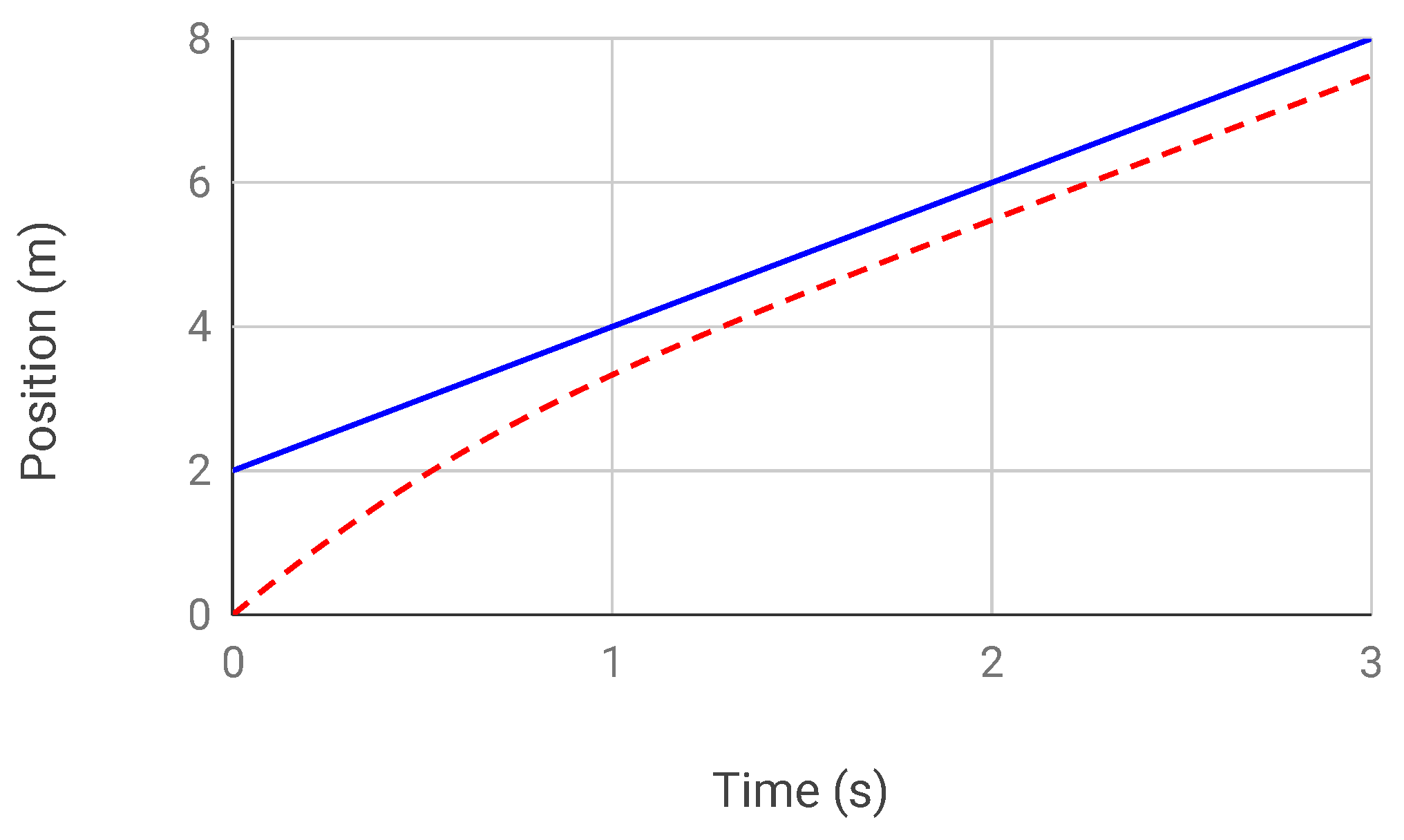
Figure 4.
In this case, due to the low capacity of the link () a faster vehicle gets stuck behind a slower vehicle.
Figure 4.
In this case, due to the low capacity of the link () a faster vehicle gets stuck behind a slower vehicle.

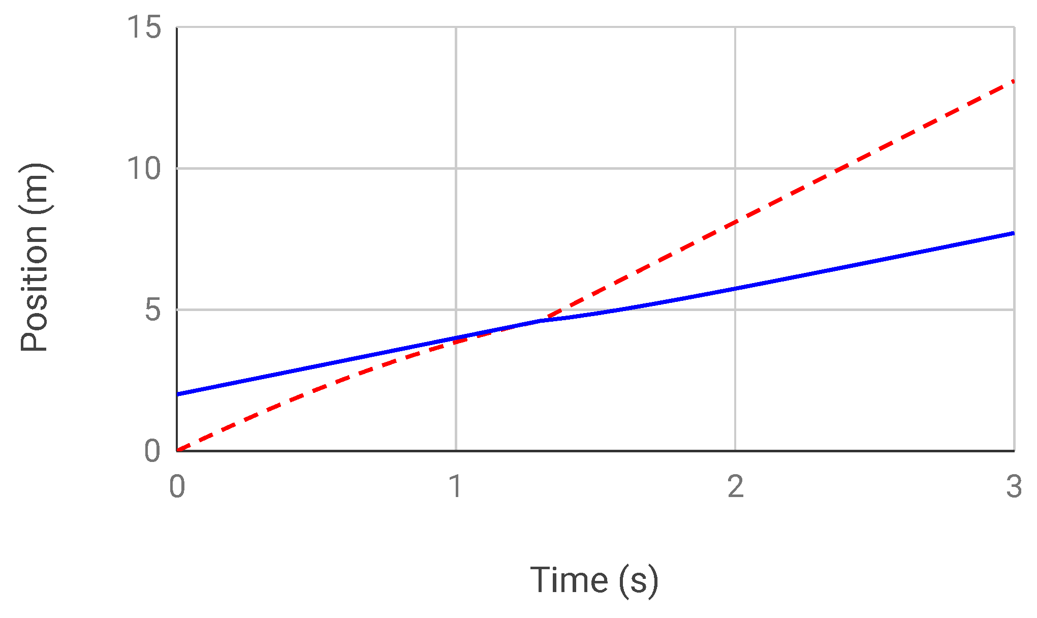
Figure 5.
In this case, the link has enough capacity () and a faster vehicle easily passes a slower vehicle.
Figure 5.
In this case, the link has enough capacity () and a faster vehicle easily passes a slower vehicle.

Figure 6.
Vehicle flow versus density: For our microscopic model, this graph shows the macroscopic relationship between the number of identical vehicles passing a fixed point on a ring road per unit of time and the density of vehicles. As is expected from a traffic flow model, after a peak density matching the available capacity is reached, traffic flow starts deteriorating in the sense that any more vehicles only serve to slow down every vehicle. Before this peak, the traffic is in the free flow regime and then switches to congested.

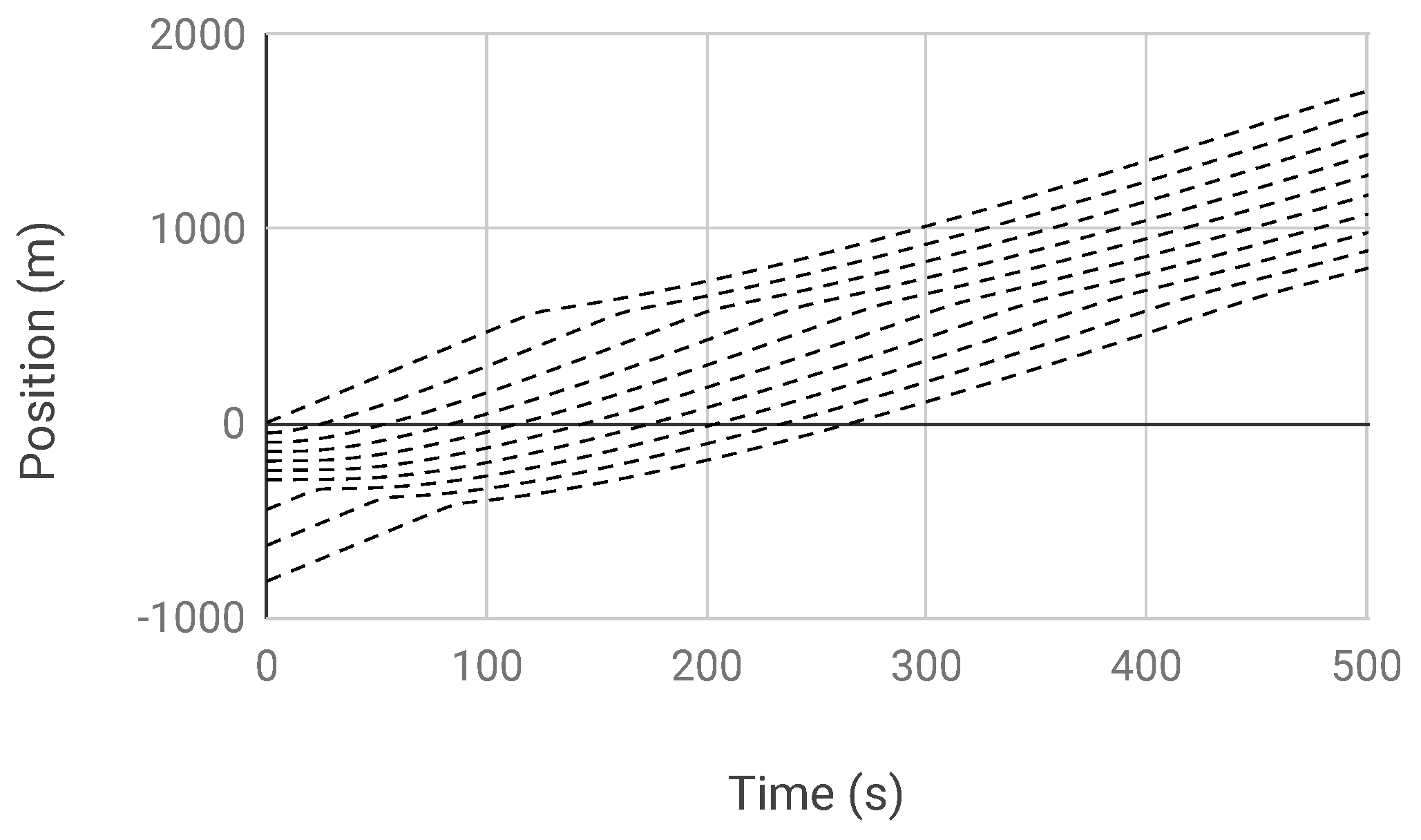
Figure 7.
Time-Space Diagram for every 50th vehicle: of the ring road has a maximal uniform vehicle density of and the remaining has a uniform density of . The ring road vehicle density is . Initially, some vehicles are slowed down, but as time goes on, all the velocities converge to the equilibrium velocity.

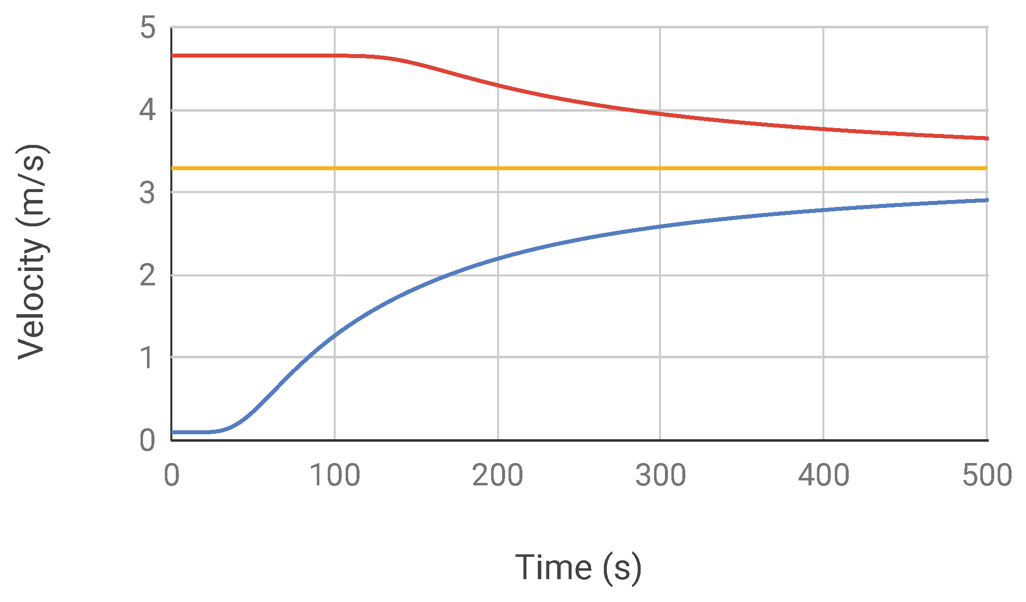
Figure 8.
Minimum and maximum momentary velocity among all vehicles: of the ring road has a maximal uniform vehicle density of and the remaining has a uniform density of . The ring road vehicle density is . This graph shows the convergence to equilibrium velocity.
Figure 8.
Minimum and maximum momentary velocity among all vehicles: of the ring road has a maximal uniform vehicle density of and the remaining has a uniform density of . The ring road vehicle density is . This graph shows the convergence to equilibrium velocity.


Table 1.
Effect of capacity () on the model’s behavior.
| Capacity () | Model’s Behavior |
|---|---|
| Low: | Blocking regime: No vehicle can pass |
| Medium: | Passing regime: Initial position of vehicles determines the final ordering; that is which vehicles will end up passing |
| High: | Passing regime: All faster vehicles end up ahead of slower ones |
Publisher’s Note: MDPI stays neutral with regard to jurisdictional claims in published maps and institutional affiliations. |
© 2021 by the authors. Licensee MDPI, Basel, Switzerland. This article is an open access article distributed under the terms and conditions of the Creative Commons Attribution (CC BY) license (https://creativecommons.org/licenses/by/4.0/).
Share and Cite
MDPI and ACS Style
Gharibi, M.; Gharibi, Z.; Boutaba, R.; Waslander, S.L. A Density-Based and Lane-Free Microscopic Traffic Flow Model Applied to Unmanned Aerial Vehicles. Drones 2021, 5, 116. https://doi.org/10.3390/drones5040116
AMA Style
Gharibi M, Gharibi Z, Boutaba R, Waslander SL. A Density-Based and Lane-Free Microscopic Traffic Flow Model Applied to Unmanned Aerial Vehicles. Drones. 2021; 5(4):116. https://doi.org/10.3390/drones5040116
Chicago/Turabian StyleGharibi, Mirmojtaba, Zahra Gharibi, Raouf Boutaba, and Steven L. Waslander. 2021. "A Density-Based and Lane-Free Microscopic Traffic Flow Model Applied to Unmanned Aerial Vehicles" Drones 5, no. 4: 116. https://doi.org/10.3390/drones5040116