
Ensemble-Based Classification Using Neural Networks and Machine Learning Models for Windows PE Malware Detection

 , , and
Abstract
:1. Introduction
- (1)
- The detailed experimental analysis and verification of machine learning and deep learning methods for malware recognition performed on the Classification of Malware with PE headers (ClaMP) dataset;
- (2)
- A novel ensemble learning-based hybrid classification framework for malware detection with a heterogeneous batch of convolutional neural networks (CNNs) as base classifiers and a machine learning algorithm as a final-stage classifier, which allows us to achieve the improvement of malware detection accuracy;
- (3)
- An extensive ablation study to select CNN model architectures and a machine learning algorithm for the best overall malware detection performance.
2. Related Works
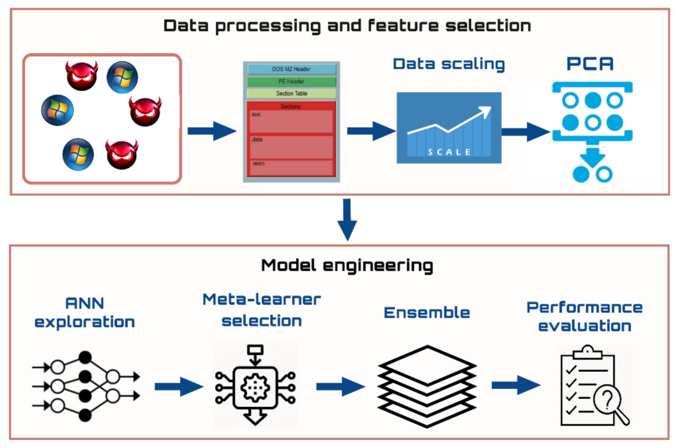
3. Materials and Methods
3.1. Data Collection and Processing
- -
- DOS image header: e_cp–pages in file, e_cblp–bytes on the last page, e_cparhdr–size of header, e_crlc–number of relocations, e_cs–initial CS value, e_csum - checksum, e_ip–initial IP value, e_lfanewe_lfarlc, e_magic–Magic number, e_maxalloc–maximum extra paragraphs, e_minalloc–minimum number of extra paragraphs, e_oemid–OEM ID, e_oeminfo–OEM information, e_ovno–overlay number, e_res and e_res2–reserved words, e_sp–initial SP value, e_ss–initial SS value.
- -
- File header features: CharacteristicsCreationYear, Machine, NumberOfSections, NumberOfSymbols, PointerToSymbolTable, SizeOfOptionalHeader.
- -
- Other raw features: AddressOfEntryPoint, BaseOfCode, BaseOfData, CheckSum, DllCharacteristics, FileAlignment, ImageBase, LoaderFlags, Magic, MajorImageVersion, MajorLinkerVersion, MajorOperatingSystemVersion, MajorSubsystemVersion, MinorImageVersion, MinorLinkerVersion, MinorOperatingSystemVersion, MinorSubsystemVersion, NumberOfRvaAndSizes, SectionAlignment, SizeOfCode, SizeOfHeaders, SizeOfHeapCommit, SizeOfHeapReserve, SizeOfImage, SizeOfInitializedData, SizeOfStackCommit, SizeOfStackReserve, SizeOfUninitializedData, Subsystem.
- -
- Derived features: sus_sections, non_sus_sections, packer, packer_type, E_text, E_data, filesize, E_file, fileinfo.
3.2. Dimensionality Reduction
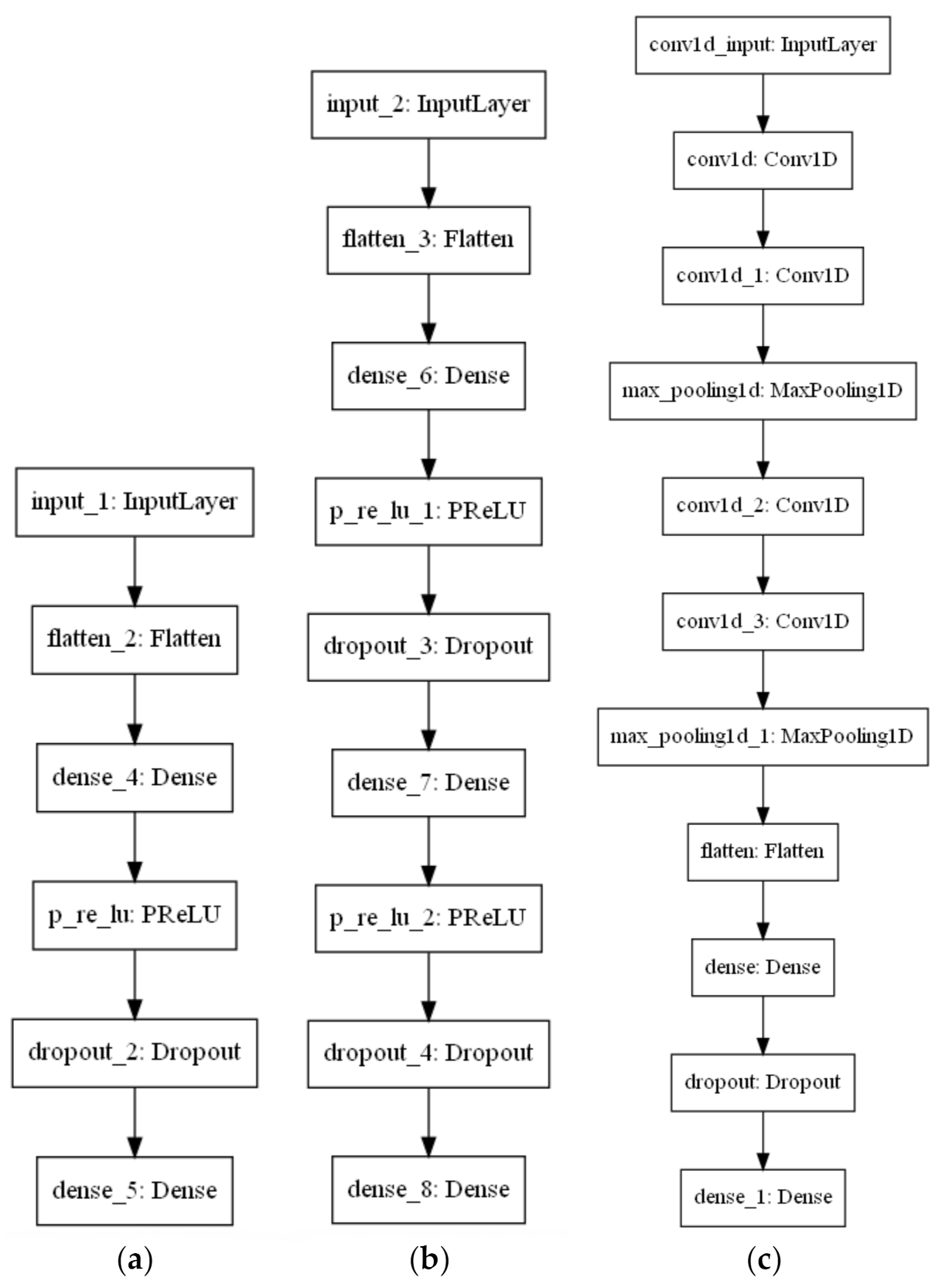
3.3. Deep Learning Models
3.3.1. Multilayer Perceptron
3.3.2. One-Dimensional Convolutional Neural Network (1D-CNN)
3.4. Network Model Optimization
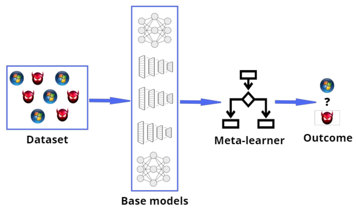
3.5. Ensemble Classification
- Set up the ensemble:
- (a)
- Select base learners;
- (b)
- Select a meta-learning algorithm.
- Train the ensemble:
- (a)
- Train each of the base learners on the training dataset , where is the number of samples;
- (b)
- Perform the k-fold cross-validation on each of the base learners and record the cross-validated predictions
- (c)
- Combine cross-validated predictions from base learners to form a new feature matrix as follows. Train the meta-learner on the new data (features x predictions from base-level classifiers) . Combine base learning models and the meta-learner to generate more accurate predictions on unknown data.
- Test on new data:
- (a)
- Record output decisions from the base learners;
- (b)
- Send base-level decisions to the meta-learner to make ensemble decision.
3.6. Evaluation of Malware Detection Results
4. Implementation and Results
4.1. Experimental Settings
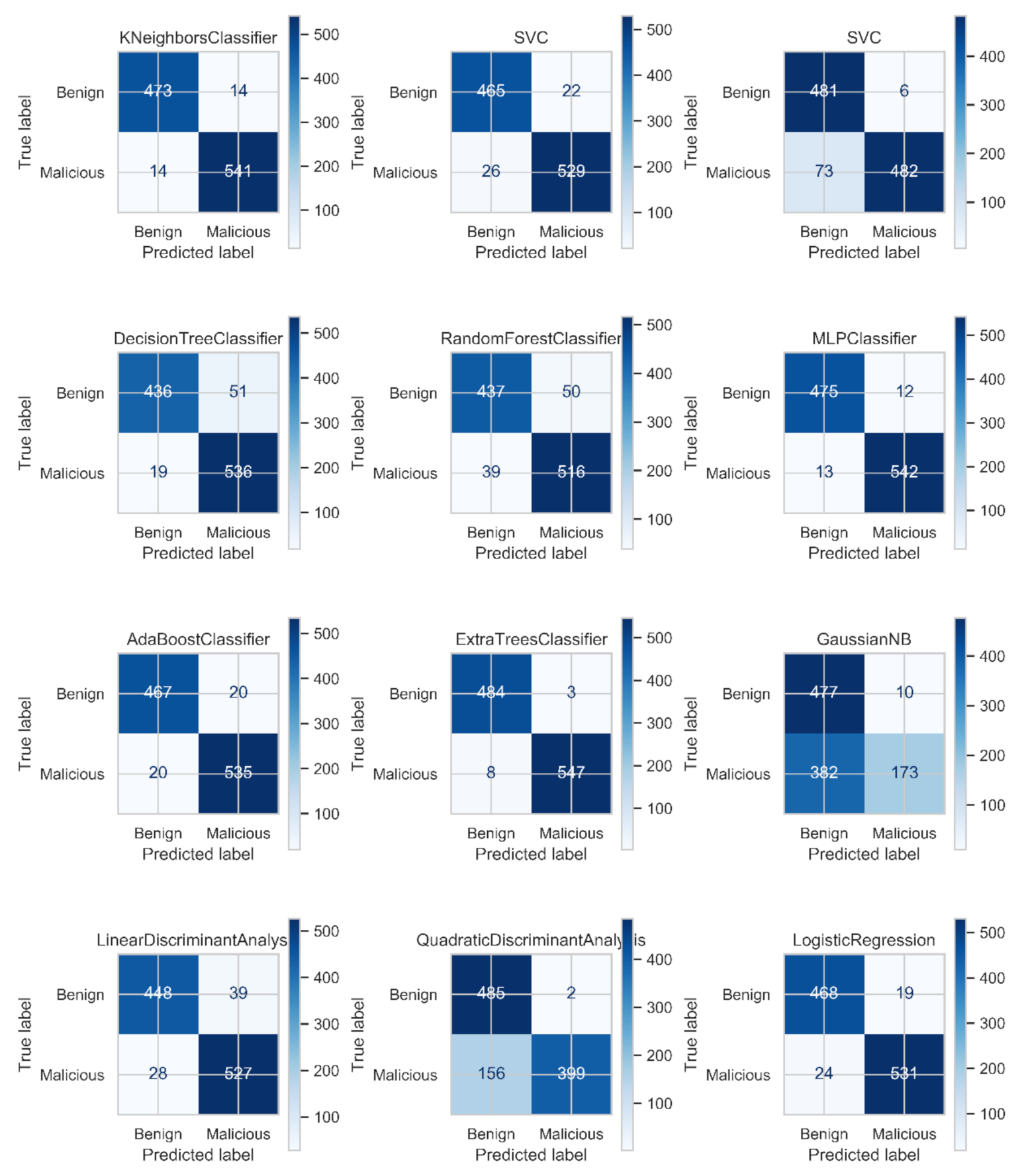
4.2. Results of Machine Learning Methods
4.3. Results of Neural Network Classifiers
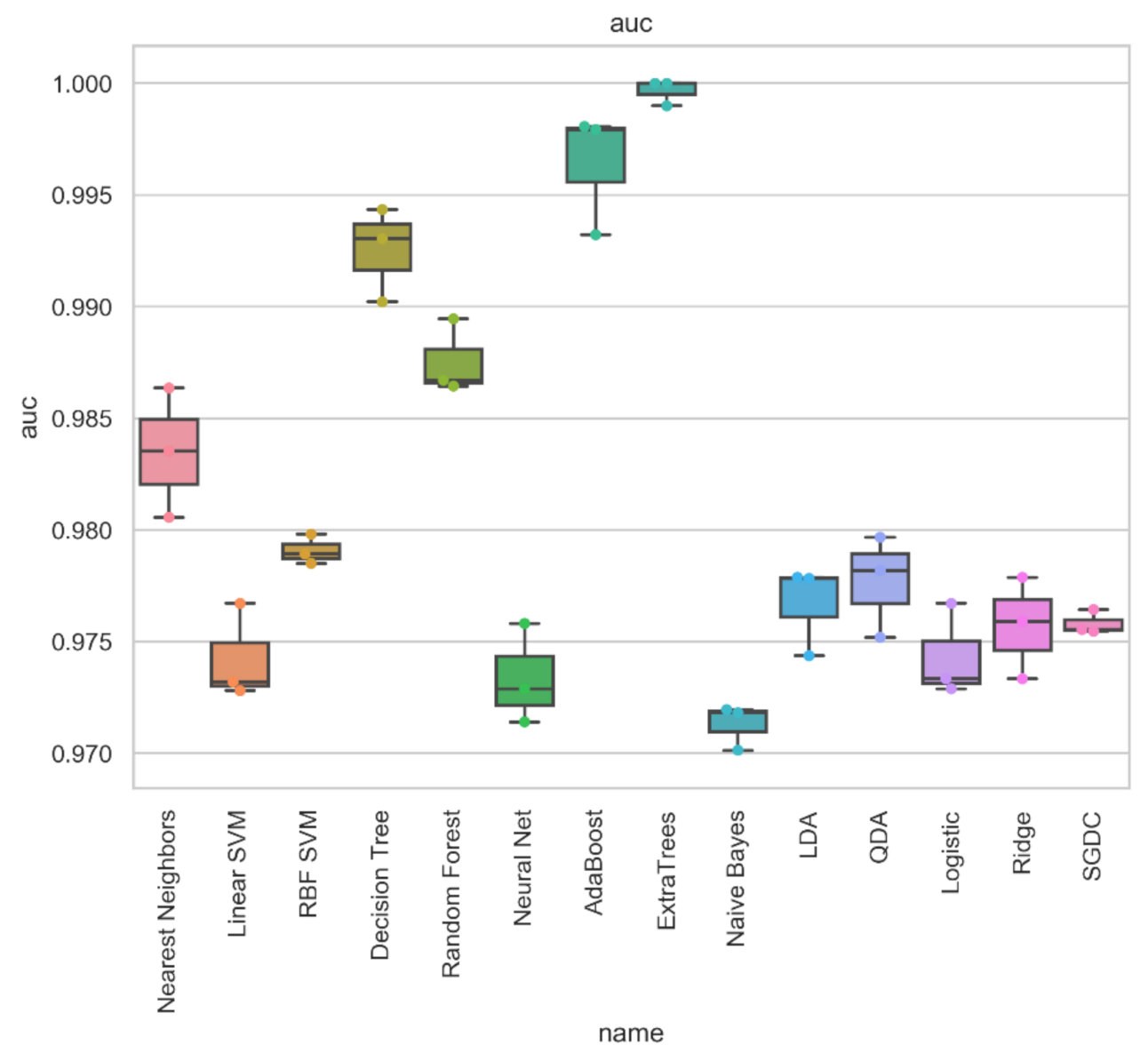
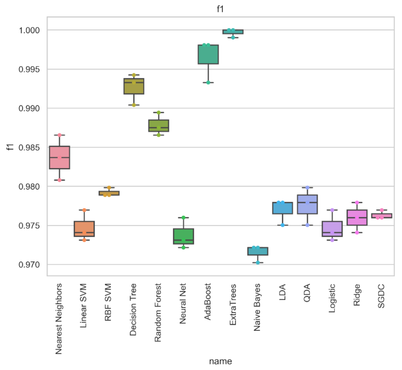
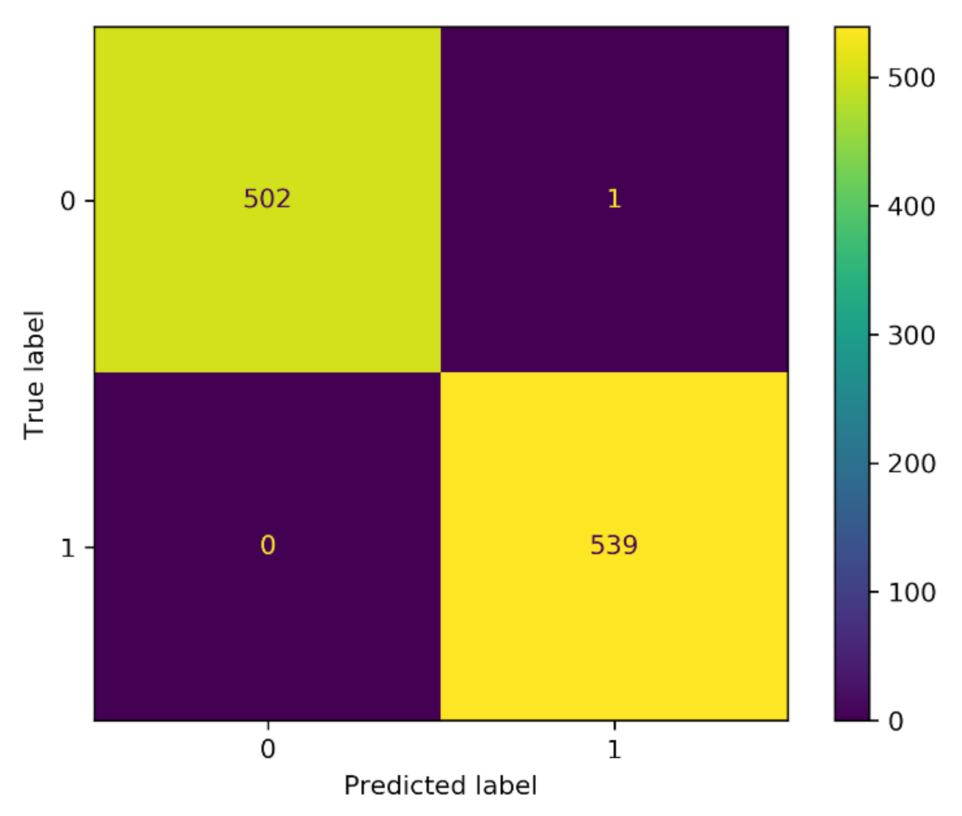
4.4. Results of Ensemble Learning
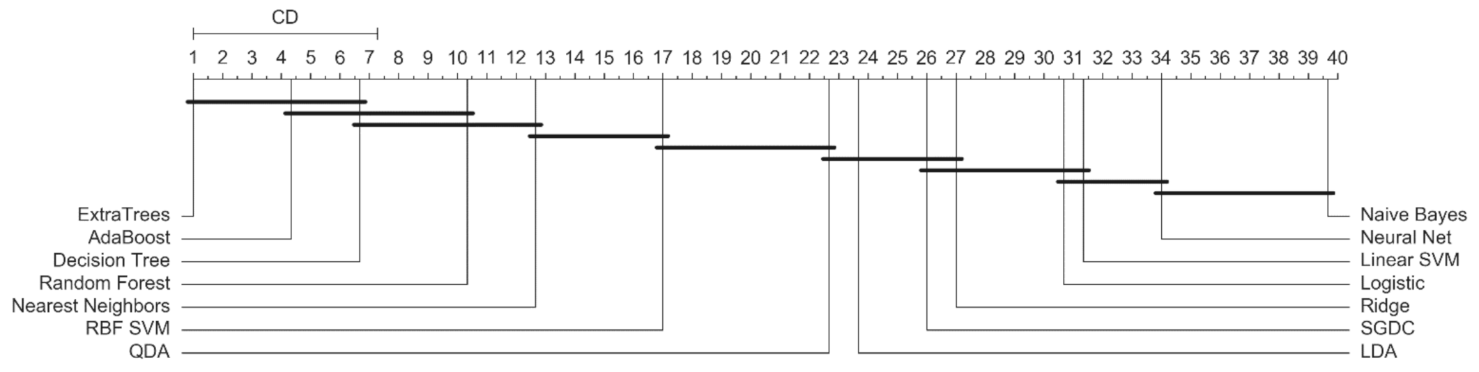
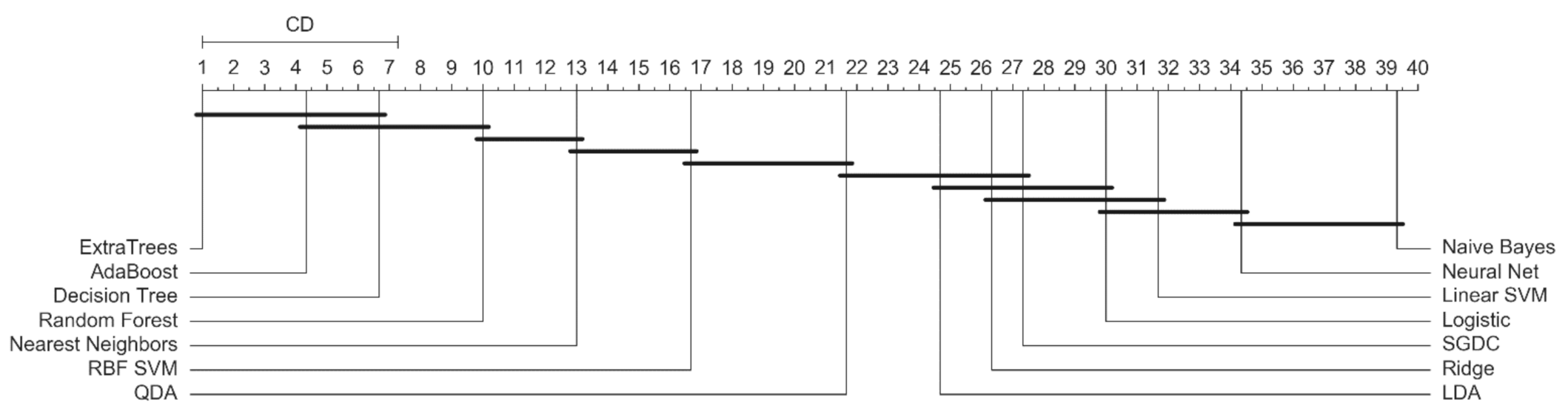
4.5. Statistical Analysis
4.6. Ablation Study of the Ensemble
- Case ENSEMBLE1: two Dense-2 (with (40,40) and (40,50) neurons) models and two 1D-CNN (with (25,25) and (30,35) neurons) models;
- Case ENSEMBLE2: one Dense-1 (with 35 neurons) model, one Dense-2 (with (40,40) neurons) model and two 1D-CNN ((25,25), and (30,35) neurons) models;
- Case ENSEMBLE3: one Dense-1 (with 35 neurons) model, two Dense-2 (with (40,40) and (40,50) neurons) models and one 1D-CNN (with (30;35) neurons) model.
4.7. Comparison with Related Work

| Reference | Benign | Malware | Acc. (%) | Prec. (%) | Recall (%) | F-Score (%) |
|---|---|---|---|---|---|---|
| Alzaylaee et al. [54] | 19,620 | 11,505 | 98.5 | 98.09 | 99.56 | 98.82 |
| Bakour and Ünver [55] | - | 4850 | 98.14 | n/a | n/a | n/a |
| Cai et al. [56] | 3000 | 3000 | 96.92 | 96.75 | 97.23 | 96.99 |
| Chen et al. [57] | 4596 | 4596 | 97.23 | 98.69 | 98.69 | 98.69 |
| Fang et al. [58] | 749 | 726 | n/a | n/a | 98.07 | n/a |
| Imtiaz et al. [59] | 5065 | 426 | 93.4 | 93.5 | 93.4 | 93.2 |
| Jeon and Moon [60] | 1000 | 1000 | 96 | n/a | 95 | n/a |
| Jha et al. [61] | 20,000 | 20,000 | 91.91 | n/a | n/a | 91.76 |
| Namavar Jahromi et al. [62] | - | 18,831 | 99.03 | n/a | n/a | n/a |
| Narayanan and Davuluru [63] | - | 7826 | 99.8 | n/a | n/a | n/a |
| Song et al. [64] | 30,487 | 29,893 | 97.71 | n/a | n/a | 98.29 |
| Wang et al. [65] | 6375 | 6375 | n/a | 94 | n/a | n/a |
| Yen and Sun [66] | 720 | 720 | 92.67 | n/a | n/a | n/a |
| This paper | 2488 | 2722 | 99.99 | 99.99 | 99.98 | 99.99 |
5. Conclusions
Author Contributions
Funding
Data Availability Statement
Conflicts of Interest
References
- Lallie, H.S.; Shepherd, L.A.; Nurse, J.R.C.; Erola, A.; Epiphaniou, G.; Maple, C.; Bellekens, X.J.A. Cyber Security in the Age of COVID-19: A Timeline and Analysis of Cyber-Crime and Cyber-Attacks during the Pandemic. arXiv 2020, arXiv:2006.11929. [Google Scholar]
- Anderson, R.; Barton, C.; Böhme, R.; Clayton, R.; Van Eeten, M.J.G.; Levi, M.; Moore, T.; Savage, S. Measuring the Cost of Cybercrime. In The Economics of Information Security and Privacy; Springer: Berlin/Heidelberg, Germany, 2013; pp. 265–300. [Google Scholar]
- Bissell, K.; la Salle, R.; Dal, C.P. The 2020 Cyber Security Report. 2020. Available online: https://pages.checkpoint.com/cyber-security-report-2020 (accessed on 4 May 2020).
- Chebyshev, V. Mobile Malware Evolution. 2018. Available online: https://securelist.com/mobile-malware-evolution-2018/89689/ (accessed on 18 June 2020).
- Kaspersky Lab. The Great Bank Robbery. 2015. Available online: https://www.kaspersky.com/about/press-releases/2015_the-great-bank-robbery-carbanak-cybergang-steals--1bn-from-100-financial-institutions-worldwide (accessed on 17 February 2015).
- Kingsoft. 2015–2016 Internet Security Research Report in China. 2016. Available online: https://cn.cmcm.com/news/media/2016-01-14/60.html (accessed on 14 January 2016).
- Bissell, K.; la Salle, R.M.; Dal, C.P. The Cost of Cybercrime—Ninth Annual Cost of Cybercrime Study. Technical Report, Ponemon Institute LLC, Accenture. 2019. Available online: https://www.accenture.com/_acnmedia/pdf-96/accenture-2019-cost-of-cybercrime-study-final.pdf (accessed on 3 March 2020).
- Cybersecurity Ventures. Cybercrime Damages Will Cost the World $6 Trillion Annually by 2021. 2017. Available online: https://cybersecurityventures.com/cybercrime-damages-6-trillion-by-2021/ (accessed on 21 December 2020).
- Williams, C.M.; Chaturvedi, R.; Chakravarthy, K. Cybersecurity Risks in a Pandemic. J. Med. Internet Res. 2020, 22, e23692. [Google Scholar] [CrossRef]
- Hakak, S.; Khan, W.Z.; Imran, M.; Choo, K.-K.R.; Shoaib, M. Have You Been a Victim of COVID-19-Related Cyber Incidents? Survey, Taxonomy, and Mitigation Strategies. IEEE Access 2020, 8, 124134–124144. [Google Scholar] [CrossRef]
- Seh, A.H.; Zarour, M.; Alenezi, M.; Sarkar, A.K.; Agrawal, A.; Kumar, R.; Khan, R.A. Healthcare Data Breaches: Insights and Implications. Healthcare 2020, 8, 133. [Google Scholar] [CrossRef]
- Pierazzi, F.; Mezzour, G.; Han, Q.; Colajanni, M.; Subrahmanian, V.S. A Data-driven Characterization of Modern Android Spyware. ACM Trans. Manag. Inf. Syst. 2020, 11, 1–38. [Google Scholar] [CrossRef] [Green Version]
- Odusami, M.; Abayomi-Alli, O.; Misra, S.; Shobayo, O.; Damasevicius, R.; Maskeliunas, R. Android Malware Detection: A Survey. In Communications in Computer and Information Science; Springer International Publishing: Cham, Switzerland, 2018; Volume 942, pp. 255–266. [Google Scholar] [CrossRef]
- Subairu, S.O.; Alhassan, J.; Misra, S.; Abayomi-Alli, O.; Ahuja, R.; Damasevicius, R.; Maskeliunas, R. An Experimental Approach to Unravel Effects of Malware on System Network Interface. In Lecture Notes in Electrical Engineering; Springer International Publishing: Cham, Switzerland, 2019; Volume 612, pp. 225–235. [Google Scholar] [CrossRef]
- Alsoghyer, S.; Almomani, I. Ransomware Detection System for Android Applications. Electronics 2019, 8, 868. [Google Scholar] [CrossRef] [Green Version]
- Hindy, H.; Atkinson, R.; Tachtatzis, C.; Colin, J.-N.; Bayne, E.; Bellekens, X. Utilising Deep Learning Techniques for Effective Zero-Day Attack Detection. Electronics 2020, 9, 1684. [Google Scholar] [CrossRef]
- Martín, I.; Hernández, J.A.; Santos, S.D.L. Machine-Learning based analysis and classification of Android malware signatures. Futur. Gener. Comput. Syst. 2019, 97, 295–305. [Google Scholar] [CrossRef]
- Aslan, O.; Samet, R. A Comprehensive Review on Malware Detection Approaches. IEEE Access 2020, 8, 6249–6271. [Google Scholar] [CrossRef]
- Souri, A.; Hosseini, R. A state-of-the-art survey of malware detection approaches using data mining techniques. Hum. Cent. Comput. Inf. Sci. 2018, 8, 3. [Google Scholar] [CrossRef]
- Ye, Y.; Li, T.; Adjeroh, D.; Iyengar, S.S. A Survey on Malware Detection Using Data Mining Techniques. ACM Comput. Surv. 2017, 50, 1–40. [Google Scholar] [CrossRef]
- Ucci, D.; Aniello, L.; Baldoni, R. Survey of machine learning techniques for malware analysis. Comput. Secur. 2019, 81, 123–147. [Google Scholar] [CrossRef] [Green Version]
- Liu, K.; Xu, S.; Xu, G.; Zhang, M.; Sun, D.; Liu, H. A Review of Android Malware Detection Approaches Based on Machine Learning. IEEE Access 2020, 8, 124579–124607. [Google Scholar] [CrossRef]
- Truong, T.C.; Diep, Q.B.; Zelinka, I. Artificial Intelligence in the Cyber Domain: Offense and Defense. Symmetry 2020, 12, 410. [Google Scholar] [CrossRef] [Green Version]
- Ngo, Q.-D.; Nguyen, H.-T.; Le, V.-H.; Nguyen, D.-H. A survey of IoT malware and detection methods based on static features. ICT Express 2020, 6, 280–286. [Google Scholar] [CrossRef]
- Egele, M.; Scholte, T.; Kirda, E.; Kruegel, C. A survey on automated dynamic malware-analysis techniques and tools. ACM Comput. Surv. 2012, 44, 1–42. [Google Scholar] [CrossRef]
- Ye, Y.; Wang, D.; Li, T.; Ye, D.; Jiang, Q. An intelligent PE-malware detection system based on association mining. J. Comput. Virol. 2008, 4, 323–334. [Google Scholar] [CrossRef]
- Nisa, M.; Shah, J.H.; Kanwal, S.; Raza, M.; Khan, M.A.; Damaševičius, R.; Blažauskas, T. Hybrid Malware Classification Method Using Segmentation-Based Fractal Texture Analysis and Deep Convolution Neural Network Features. Appl. Sci. 2020, 10, 4966. [Google Scholar] [CrossRef]
- Yong, B.; Wei, W.; Li, K.; Shen, J.; Zhou, Q.; Wozniak, M.; Połap, D.; Damaševičius, R. Ensemble machine learning approaches for webshell detection in Internet of things environments. Trans. Emerg. Telecommun. Technol. 2020. [Google Scholar] [CrossRef]
- Wei, W.; Woźniak, M.; Damaševičius, R.; Fan, X.; Li, Y. Algorithm research of known-plaintext attack on double random phase mask based on WSNs. J. Internet Technol. 2019, 20, 39–48. [Google Scholar] [CrossRef]
- Berman, D.S.; Buczak, A.L.; Chavis, J.S.; Corbett, C.L. A Survey of Deep Learning Methods for Cyber Security. Information 2019, 10, 122. [Google Scholar] [CrossRef] [Green Version]
- Ren, Z.; Wu, H.; Ning, Q.; Hussain, I.; Chen, B. End-to-end malware detection for android IoT devices using deep learning. Ad Hoc Netw. 2020, 101, 102098. [Google Scholar] [CrossRef]
- Yuxin, D.; Siyi, Z. Malware detection based on deep learning algorithm. Neural Comput. Appl. 2017, 31, 461–472. [Google Scholar] [CrossRef]
- Pei, X.; Yu, L.; Tian, S. AMalNet: A deep learning framework based on graph convolutional networks for malware detection. Comput. Secur. 2020, 93, 101792. [Google Scholar] [CrossRef]
- Čeponis, D.; Goranin, N. Investigation of Dual-Flow Deep Learning Models LSTM-FCN and GRU-FCN Efficiency against Single-Flow CNN Models for the Host-Based Intrusion and Malware Detection Task on Univariate Times Series Data. Appl. Sci. 2020, 10, 2373. [Google Scholar] [CrossRef] [Green Version]
- Huang, X.; Ma, L.; Yang, W.; Zhong, Y. A Method for Windows Malware Detection Based on Deep Learning. J. Signal Process. Syst. 2020, 1–9. [Google Scholar] [CrossRef]
- Martins, N.; Cruz, J.M.; Cruz, T.; Abreu, P.H. Adversarial Machine Learning Applied to Intrusion and Malware Scenarios: A Systematic Review. IEEE Access 2020, 8, 35403–35419. [Google Scholar] [CrossRef]
- Zador, A.M. A critique of pure learning and what artificial neural networks can learn from animal brains. Nat. Commun. 2019, 10, 1–7. [Google Scholar] [CrossRef] [PubMed] [Green Version]
- Idrees, F.; Rajarajan, M.; Conti, M.; Chen, T.M.; Rahulamathavan, Y. PIndroid: A novel Android malware detection system using ensemble learning methods. Comput. Secur. 2017, 68, 36–46. [Google Scholar] [CrossRef] [Green Version]
- Feng, P.; Ma, J.; Sun, C.; Xu, X.; Ma, Y. A Novel Dynamic Android Malware Detection System with Ensemble Learning. IEEE Access 2018, 6, 30996–31011. [Google Scholar] [CrossRef]
- Wang, W.; Li, Y.; Wang, X.; Liu, J.; Zhang, X. Detecting Android malicious apps and categorizing benign apps with ensemble of classifiers. Futur. Gener. Comput. Syst. 2018, 78, 987–994. [Google Scholar] [CrossRef] [Green Version]
- Yan, J.; Qi, Y.; Rao, Q. Detecting Malware with an Ensemble Method Based on Deep Neural Networks. Secur. Commun. Netw. 2018, 2018, 1–16. [Google Scholar] [CrossRef] [Green Version]
- Gupta, D.; Rani, R. Improving malware detection using big data and ensemble learning. Comput. Electr. Eng. 2020, 86, 106729. [Google Scholar] [CrossRef]
- Sagi, O.; Rokach, L. Ensemble learning: A survey. Wiley Interdiscip. Rev. Data Min. Knowl. Discov. 2018, 8, e1249. [Google Scholar] [CrossRef]
- Basu, I. Malware detection based on source data using data mining: A survey. Am. J. Adv. Comput. 2016, 3, 18–37. [Google Scholar]
- Srivastava, N.; Hinton, G.; Krizhevsky, A.; Sutskever, I.; Salakhutdinov, R. Dropout: A simple way to prevent neural networks from overfitting. J. Mach. Learn. Res. 2014, 15, 1929–1958. [Google Scholar]
- Ruder, S. An overview of gradient descent optimization algorithms. arXiv 2016, arXiv:1609.04747. [Google Scholar]
- Duchi, J.; Hazan, E.; Singer, Y. Adaptive subgradient methods for online learning and stochastic optimization. J. Mach. Learn. Res. 2011, 12, 2121–2159. [Google Scholar]
- Tieleman, T.; Hinton, G. Lecture 6.5-rmsprop: Divide the gradient by a running average of its recent magnitude. Coursera Neural Netw. Mach. Learn. 2012, 4, 26–31. [Google Scholar]
- Kingma, D.P.; Ba, J. Adam: A method for stochastic optimization. In Proceedings of the International Conference on Learning Representation (ICLR), San Diego, CA, USA, 5–8 May 2015. [Google Scholar]
- Ragab, M.; Abdulkadir, S.; Aziz, N.; Al-Tashi, Q.; Alyousifi, Y.; Alhussian, H.; Alqushaibi, A. A Novel One-Dimensional CNN with Exponential Adaptive Gradients for Air Pollution Index Prediction. Sustainability 2020, 12, 10090. [Google Scholar] [CrossRef]
- Luo, L.; Xiong, Y.; Liu, Y.; Sun, X. Adaptive gradient methods with dynamic bound of learning rate. arXiv 2019, arXiv:1902.09843. [Google Scholar]
- Van der Laan, M.J.; Polley, E.C.; Hubbard, A.E. Super Learner. Stat. Appl. Genet. Mol. Biol. 2007, 6. [Google Scholar] [CrossRef] [PubMed]
- Geurts, P.; Ernst, D.; Wehenkel, L. Extremely randomized trees. Mach. Learn. 2006, 63, 3–42. [Google Scholar] [CrossRef] [Green Version]
- Alzaylaee, M.K.; Yerima, S.Y.; Sezer, S. DL-Droid: Deep learning based android malware detection using real devices. Comput. Secur. 2020, 89, 101663. [Google Scholar] [CrossRef]
- Bakour, K.; Ünver, H.M. VisDroid: Android malware classification based on local and global image features, bag of visual words and machine learning techniques. Neural Comput. Appl. 2020, 2020, 1–21. [Google Scholar] [CrossRef]
- Cai, L.; Li, Y.; Xiong, Z. JOWMDroid: Android malware detection based on feature weighting with joint optimization of weight-mapping and classifier parameters. Comput. Secur. 2021, 100, 102086. [Google Scholar] [CrossRef]
- Chen, J.; Guo, S.; Ma, X.; Li, H.; Guo, J.; Chen, M.; Pan, Z. SLAM: A Malware Detection Method Based on Sliding Local Attention Mechanism. Secur. Commun. Netw. 2020, 2020, 1–11. [Google Scholar] [CrossRef]
- Fang, Y.; Zeng, Y.; Li, B.; Liu, L.; Zhang, L. DeepDetectNet vs RLAttackNet: An adversarial method to improve deep learning-based static malware detection model. PLoS ONE 2020, 15, e0231626. [Google Scholar] [CrossRef]
- Imtiaz, S.I.; Rehman, S.U.; Javed, A.R.; Jalil, Z.; Liu, X.; Alnumay, W.S. DeepAMD: Detection and identification of Android malware using high-efficient Deep Artificial Neural Network. Futur. Gener. Comput. Syst. 2021, 115, 844–856. [Google Scholar] [CrossRef]
- Jeon, S.; Moon, J. Malware-Detection Method with a Convolutional Recurrent Neural Network Using Opcode Sequences. Inf. Sci. 2020, 535, 1–15. [Google Scholar] [CrossRef]
- Jha, S.; Prashar, D.; Long, H.V.; Taniar, D. Recurrent neural network for detecting malware. Comput. Secur. 2020, 99, 102037. [Google Scholar] [CrossRef]
- Jahromi, A.N.; Hashemi, S.; Dehghantanha, A.; Choo, K.-K.R.; Karimipour, H.; Newton, D.E.; Parizi, R.M. An improved two-hidden-layer extreme learning machine for malware hunting. Comput. Secur. 2020, 89, 101655. [Google Scholar] [CrossRef]
- Narayanan, B.N.; Davuluru, V.S.P. Ensemble Malware Classification System Using Deep Neural Networks. Electronics 2020, 9, 721. [Google Scholar] [CrossRef]
- Song, X.; Chen, C.; Cui, B.; Fu, J. Malicious JavaScript Detection Based on Bidirectional LSTM Model. Appl. Sci. 2020, 10, 3440. [Google Scholar] [CrossRef]
- Wang, X.; Li, C.; Song, D.; Wang, C. CrowdNet: Identifying Large-Scale Malicious Attacks Over Android Kernel Structures. IEEE Access 2020, 8, 15823–15837. [Google Scholar] [CrossRef]
- Yen, Y.-S.; Sun, H.-M. An Android mutation malware detection based on deep learning using visualization of importance from codes. Microelectron. Reliab. 2019, 93, 109–114. [Google Scholar] [CrossRef]
- Zanni-Merk, C. On the Need of an Explainable Artificial Intelligence. In Proceedings of the 40th Anniversary International Conference on Information Systems Architecture and Technology, Wroclaw, Poland, 15–17 September 2019; p. 3. [Google Scholar]


| Dense-1 Network | Dense-2 Network | 1D-CNN Network |
|---|---|---|
| Parameters | ||
| X—number of neurons in 1st hidden layer | X—number of neurons in 1st hidden layer Y—number of neurons in 2nd hidden layer | F—number of filters in convolutional layers N—number of neurons in dense layer |
| Input layer of 40 × 1 features | ||
| 1 FC layer (X neurons) | 1 FC layer (X neurons) | 2 Conv1D layers (F 2 × 2 filters) |
| PReLU | PReLU | Max-pooling layer |
| Dropout layer (p = 0.3) | Dropout layer (p = 0.3) | 2 Conv1D layers (F 2 × 2 filters) |
| 1 FC layer (2 neurons) | 1 FC layer (Y neurons) | Max-pooling layer |
| Softmax output layer | PReLU | 1 FC layer (N neurons) |
| Dropout layer (p = 0.3) | Dropout layer (p = 0.5) | |
| 1 FC layer (2 neurons) | 1 FC layer (2 neurons) | |
| Softmax output layer | Softmax output layer | |
| Meta-Learner | Acc | Prec | Rec | Spec | FPR | FNR | F1 | AUC | MCC | Kappa |
|---|---|---|---|---|---|---|---|---|---|---|
| Nearest Neighbors | 0.973 | 0.973 | 0.973 | 0.973 | 0.029 | 0.025 | 0.973 | 0.973 | 0.946 | 0.946 |
| Linear SVM | 0.954 | 0.954 | 0.954 | 0.954 | 0.045 | 0.047 | 0.954 | 0.954 | 0.908 | 0.908 |
| RBF SVM | 0.924 | 0.924 | 0.924 | 0.924 | 0.012 | 0.132 | 0.924 | 0.928 | 0.856 | 0.849 |
| Decision Tree | 0.933 | 0.933 | 0.933 | 0.933 | 0.107 | 0.032 | 0.933 | 0.93 | 0.866 | 0.864 |
| Random Forest | 0.931 | 0.931 | 0.931 | 0.931 | 0.08 | 0.059 | 0.931 | 0.93 | 0.861 | 0.861 |
| Neural Net | 0.977 | 0.977 | 0.977 | 0.977 | 0.021 | 0.025 | 0.977 | 0.977 | 0.954 | 0.954 |
| AdaBoost | 0.962 | 0.962 | 0.962 | 0.962 | 0.041 | 0.036 | 0.962 | 0.961 | 0.923 | 0.923 |
| ExtraTrees | 0.988 | 0.988 | 0.988 | 0.988 | 0.008 | 0.014 | 0.988 | 0.989 | 0.977 | 0.977 |
| LDA | 0.936 | 0.936 | 0.936 | 0.936 | 0.08 | 0.05 | 0.936 | 0.935 | 0.871 | 0.871 |
| Logistic | 0.959 | 0.959 | 0.959 | 0.959 | 0.039 | 0.043 | 0.959 | 0.959 | 0.917 | 0.917 |
| Passive | 0.933 | 0.933 | 0.933 | 0.933 | 0.037 | 0.094 | 0.933 | 0.935 | 0.867 | 0.866 |
| Ridge | 0.936 | 0.936 | 0.936 | 0.936 | 0.08 | 0.05 | 0.936 | 0.935 | 0.871 | 0.871 |
| SGDC | 0.958 | 0.958 | 0.958 | 0.958 | 0.035 | 0.049 | 0.958 | 0.958 | 0.915 | 0.915 |
| No. of Neurons in 1st Layer | Acc | Prec | Rec | Spec | FPR | FNR | F1 | AUC | MCC | Kappa |
|---|---|---|---|---|---|---|---|---|---|---|
| 5 | 0.956 | 0.956 | 0.956 | 0.956 | 0.035 | 0.052 | 0.956 | 0.956 | 0.912 | 0.912 |
| 10 | 0.962 | 0.962 | 0.962 | 0.962 | 0.043 | 0.033 | 0.962 | 0.962 | 0.924 | 0.924 |
| 15 | 0.965 | 0.965 | 0.965 | 0.965 | 0.034 | 0.036 | 0.965 | 0.965 | 0.929 | 0.929 |
| 20 | 0.971 | 0.971 | 0.971 | 0.971 | 0.026 | 0.033 | 0.971 | 0.971 | 0.941 | 0.941 |
| 25 | 0.977 | 0.977 | 0.977 | 0.977 | 0.023 | 0.023 | 0.977 | 0.977 | 0.954 | 0.954 |
| 30 | 0.977 | 0.977 | 0.977 | 0.977 | 0.022 | 0.024 | 0.977 | 0.977 | 0.954 | 0.954 |
| 35 | 0.980 | 0.980 | 0.980 | 0.980 | 0.022 | 0.019 | 0.980 | 0.979 | 0.959 | 0.959 |
| 40 | 0.979 | 0.979 | 0.979 | 0.979 | 0.023 | 0.019 | 0.979 | 0.979 | 0.958 | 0.958 |
| No. of Neurons in 1st Layer | No. of Neurons in 2nd Layer | Acc | Prec | Rec | Spec | FPR | FNR | F1 | AUC | MCC | Kappa |
|---|---|---|---|---|---|---|---|---|---|---|---|
| 5 | 5 | 0.954 | 0.954 | 0.954 | 0.954 | 0.057 | 0.036 | 0.954 | 0.953 | 0.908 | 0.908 |
| 5 | 10 | 0.958 | 0.958 | 0.958 | 0.958 | 0.046 | 0.039 | 0.958 | 0.958 | 0.915 | 0.915 |
| 5 | 15 | 0.960 | 0.960 | 0.960 | 0.960 | 0.032 | 0.047 | 0.960 | 0.960 | 0.919 | 0.919 |
| 5 | 20 | 0.964 | 0.964 | 0.964 | 0.964 | 0.039 | 0.033 | 0.964 | 0.964 | 0.928 | 0.928 |
| 5 | 25 | 0.961 | 0.961 | 0.961 | 0.961 | 0.042 | 0.036 | 0.961 | 0.961 | 0.922 | 0.922 |
| 5 | 30 | 0.965 | 0.965 | 0.965 | 0.965 | 0.038 | 0.033 | 0.965 | 0.965 | 0.929 | 0.929 |
| 5 | 35 | 0.963 | 0.963 | 0.963 | 0.963 | 0.040 | 0.034 | 0.963 | 0.963 | 0.926 | 0.926 |
| 10 | 5 | 0.963 | 0.963 | 0.963 | 0.963 | 0.042 | 0.033 | 0.963 | 0.963 | 0.926 | 0.926 |
| 10 | 10 | 0.969 | 0.969 | 0.969 | 0.969 | 0.031 | 0.032 | 0.969 | 0.969 | 0.937 | 0.937 |
| 10 | 15 | 0.965 | 0.965 | 0.965 | 0.965 | 0.036 | 0.033 | 0.965 | 0.965 | 0.931 | 0.931 |
| 10 | 20 | 0.968 | 0.968 | 0.968 | 0.968 | 0.030 | 0.034 | 0.968 | 0.968 | 0.936 | 0.936 |
| 10 | 25 | 0.971 | 0.971 | 0.971 | 0.971 | 0.028 | 0.030 | 0.971 | 0.971 | 0.941 | 0.941 |
| 10 | 30 | 0.971 | 0.971 | 0.971 | 0.971 | 0.028 | 0.030 | 0.971 | 0.971 | 0.941 | 0.941 |
| 10 | 35 | 0.972 | 0.972 | 0.972 | 0.972 | 0.024 | 0.030 | 0.972 | 0.973 | 0.945 | 0.945 |
| 15 | 5 | 0.958 | 0.958 | 0.958 | 0.958 | 0.055 | 0.029 | 0.958 | 0.958 | 0.917 | 0.917 |
| 15 | 10 | 0.972 | 0.972 | 0.972 | 0.972 | 0.026 | 0.030 | 0.972 | 0.972 | 0.944 | 0.944 |
| 15 | 15 | 0.972 | 0.972 | 0.972 | 0.972 | 0.034 | 0.023 | 0.972 | 0.972 | 0.944 | 0.944 |
| 15 | 20 | 0.969 | 0.969 | 0.969 | 0.969 | 0.028 | 0.034 | 0.969 | 0.969 | 0.937 | 0.937 |
| 15 | 25 | 0.971 | 0.971 | 0.971 | 0.971 | 0.024 | 0.033 | 0.971 | 0.971 | 0.942 | 0.942 |
| 15 | 30 | 0.977 | 0.977 | 0.977 | 0.977 | 0.026 | 0.021 | 0.977 | 0.977 | 0.954 | 0.954 |
| 15 | 35 | 0.980 | 0.980 | 0.980 | 0.980 | 0.022 | 0.019 | 0.980 | 0.979 | 0.959 | 0.959 |
| 20 | 5 | 0.967 | 0.967 | 0.967 | 0.967 | 0.035 | 0.032 | 0.967 | 0.967 | 0.933 | 0.933 |
| 20 | 10 | 0.976 | 0.976 | 0.976 | 0.976 | 0.016 | 0.032 | 0.976 | 0.976 | 0.951 | 0.951 |
| 20 | 15 | 0.972 | 0.972 | 0.972 | 0.972 | 0.028 | 0.027 | 0.972 | 0.972 | 0.945 | 0.945 |
| 20 | 20 | 0.973 | 0.973 | 0.973 | 0.973 | 0.027 | 0.027 | 0.973 | 0.973 | 0.946 | 0.946 |
| 20 | 25 | 0.980 | 0.980 | 0.980 | 0.980 | 0.023 | 0.018 | 0.980 | 0.979 | 0.959 | 0.959 |
| 20 | 30 | 0.978 | 0.978 | 0.978 | 0.978 | 0.023 | 0.022 | 0.978 | 0.978 | 0.955 | 0.955 |
| 20 | 35 | 0.978 | 0.978 | 0.978 | 0.978 | 0.022 | 0.022 | 0.978 | 0.978 | 0.956 | 0.956 |
| 25 | 5 | 0.970 | 0.970 | 0.970 | 0.970 | 0.030 | 0.030 | 0.970 | 0.970 | 0.940 | 0.940 |
| 25 | 10 | 0.974 | 0.974 | 0.974 | 0.974 | 0.024 | 0.027 | 0.974 | 0.974 | 0.949 | 0.949 |
| 25 | 15 | 0.974 | 0.974 | 0.974 | 0.974 | 0.022 | 0.030 | 0.974 | 0.974 | 0.947 | 0.947 |
| 25 | 20 | 0.975 | 0.975 | 0.975 | 0.975 | 0.028 | 0.022 | 0.975 | 0.975 | 0.950 | 0.950 |
| 25 | 25 | 0.980 | 0.980 | 0.980 | 0.980 | 0.023 | 0.017 | 0.980 | 0.980 | 0.960 | 0.960 |
| 25 | 30 | 0.980 | 0.980 | 0.980 | 0.980 | 0.023 | 0.018 | 0.980 | 0.979 | 0.959 | 0.959 |
| 25 | 35 | 0.980 | 0.980 | 0.980 | 0.980 | 0.024 | 0.017 | 0.980 | 0.979 | 0.959 | 0.959 |
| 30 | 5 | 0.976 | 0.976 | 0.976 | 0.976 | 0.031 | 0.017 | 0.976 | 0.976 | 0.953 | 0.952 |
| 30 | 10 | 0.978 | 0.978 | 0.978 | 0.978 | 0.015 | 0.029 | 0.978 | 0.978 | 0.955 | 0.955 |
| 30 | 15 | 0.974 | 0.974 | 0.974 | 0.974 | 0.024 | 0.027 | 0.974 | 0.974 | 0.949 | 0.949 |
| 30 | 20 | 0.979 | 0.979 | 0.979 | 0.979 | 0.024 | 0.018 | 0.979 | 0.979 | 0.958 | 0.958 |
| 30 | 25 | 0.980 | 0.980 | 0.980 | 0.980 | 0.024 | 0.017 | 0.980 | 0.979 | 0.959 | 0.959 |
| 30 | 30 | 0.981 | 0.981 | 0.981 | 0.981 | 0.022 | 0.017 | 0.981 | 0.981 | 0.962 | 0.962 |
| 30 | 35 | 0.983 | 0.983 | 0.983 | 0.983 | 0.013 | 0.019 | 0.983 | 0.984 | 0.967 | 0.967 |
| No. of Filters | No. of Neurons | Acc | Prec | Rec | Spec | FPR | FNR | F1 | AUC | MCC | Kappa |
|---|---|---|---|---|---|---|---|---|---|---|---|
| 32 | 10 | 0.957 | 0.957 | 0.957 | 0.957 | 0.045 | 0.041 | 0.957 | 0.957 | 0.914 | 0.914 |
| 32 | 15 | 0.960 | 0.960 | 0.960 | 0.960 | 0.055 | 0.027 | 0.960 | 0.959 | 0.919 | 0.919 |
| 32 | 20 | 0.964 | 0.964 | 0.964 | 0.964 | 0.036 | 0.036 | 0.964 | 0.964 | 0.927 | 0.927 |
| 32 | 25 | 0.960 | 0.960 | 0.960 | 0.960 | 0.053 | 0.028 | 0.960 | 0.960 | 0.921 | 0.920 |
| 32 | 30 | 0.961 | 0.961 | 0.961 | 0.961 | 0.058 | 0.022 | 0.961 | 0.960 | 0.922 | 0.922 |
| 32 | 35 | 0.964 | 0.964 | 0.964 | 0.964 | 0.049 | 0.026 | 0.964 | 0.963 | 0.927 | 0.927 |
| 32 | 40 | 0.966 | 0.966 | 0.966 | 0.966 | 0.039 | 0.029 | 0.966 | 0.966 | 0.932 | 0.932 |
| 32 | 45 | 0.967 | 0.967 | 0.967 | 0.967 | 0.042 | 0.026 | 0.967 | 0.966 | 0.933 | 0.933 |
| 48 | 10 | 0.967 | 0.967 | 0.967 | 0.967 | 0.032 | 0.033 | 0.967 | 0.967 | 0.935 | 0.935 |
| 48 | 15 | 0.965 | 0.965 | 0.965 | 0.965 | 0.039 | 0.032 | 0.965 | 0.965 | 0.929 | 0.929 |
| 48 | 20 | 0.972 | 0.972 | 0.972 | 0.972 | 0.020 | 0.035 | 0.972 | 0.972 | 0.944 | 0.944 |
| 48 | 25 | 0.962 | 0.962 | 0.962 | 0.962 | 0.032 | 0.043 | 0.962 | 0.963 | 0.924 | 0.924 |
| 48 | 30 | 0.969 | 0.969 | 0.969 | 0.969 | 0.016 | 0.045 | 0.969 | 0.969 | 0.938 | 0.937 |
| 48 | 35 | 0.970 | 0.970 | 0.970 | 0.970 | 0.018 | 0.041 | 0.970 | 0.971 | 0.940 | 0.940 |
| 48 | 40 | 0.972 | 0.972 | 0.972 | 0.972 | 0.019 | 0.036 | 0.972 | 0.972 | 0.944 | 0.944 |
| 48 | 45 | 0.971 | 0.971 | 0.971 | 0.971 | 0.026 | 0.033 | 0.971 | 0.971 | 0.941 | 0.941 |
| 64 | 10 | 0.961 | 0.961 | 0.961 | 0.961 | 0.053 | 0.027 | 0.961 | 0.960 | 0.922 | 0.922 |
| 64 | 15 | 0.965 | 0.965 | 0.965 | 0.965 | 0.020 | 0.047 | 0.965 | 0.966 | 0.931 | 0.931 |
| 64 | 20 | 0.980 | 0.980 | 0.980 | 0.980 | 0.019 | 0.022 | 0.980 | 0.980 | 0.959 | 0.959 |
| 64 | 25 | 0.972 | 0.972 | 0.972 | 0.972 | 0.040 | 0.017 | 0.972 | 0.971 | 0.944 | 0.943 |
| 64 | 30 | 0.974 | 0.974 | 0.974 | 0.974 | 0.016 | 0.035 | 0.974 | 0.974 | 0.948 | 0.947 |
| 64 | 35 | 0.969 | 0.969 | 0.969 | 0.969 | 0.046 | 0.017 | 0.969 | 0.969 | 0.939 | 0.938 |
| 64 | 40 | 0.979 | 0.979 | 0.979 | 0.979 | 0.022 | 0.021 | 0.979 | 0.979 | 0.958 | 0.958 |
| 64 | 45 | 0.974 | 0.974 | 0.974 | 0.974 | 0.023 | 0.029 | 0.974 | 0.974 | 0.947 | 0.947 |
| 128 | 10 | 0.978 | 0.978 | 0.978 | 0.978 | 0.013 | 0.029 | 0.978 | 0.979 | 0.957 | 0.956 |
| 128 | 15 | 0.980 | 0.980 | 0.980 | 0.980 | 0.022 | 0.018 | 0.980 | 0.980 | 0.960 | 0.960 |
| 128 | 20 | 0.975 | 0.975 | 0.975 | 0.975 | 0.011 | 0.038 | 0.975 | 0.976 | 0.950 | 0.950 |
| 128 | 25 | 0.980 | 0.980 | 0.980 | 0.980 | 0.022 | 0.019 | 0.980 | 0.979 | 0.959 | 0.959 |
| 128 | 30 | 0.979 | 0.979 | 0.979 | 0.979 | 0.020 | 0.022 | 0.979 | 0.979 | 0.958 | 0.958 |
| 128 | 35 | 0.985 | 0.985 | 0.985 | 0.985 | 0.018 | 0.013 | 0.985 | 0.985 | 0.969 | 0.969 |
| 128 | 40 | 0.983 | 0.983 | 0.983 | 0.983 | 0.019 | 0.015 | 0.983 | 0.983 | 0.967 | 0.967 |
| 128 | 45 | 0.979 | 0.979 | 0.979 | 0.979 | 0.013 | 0.028 | 0.979 | 0.979 | 0.958 | 0.958 |
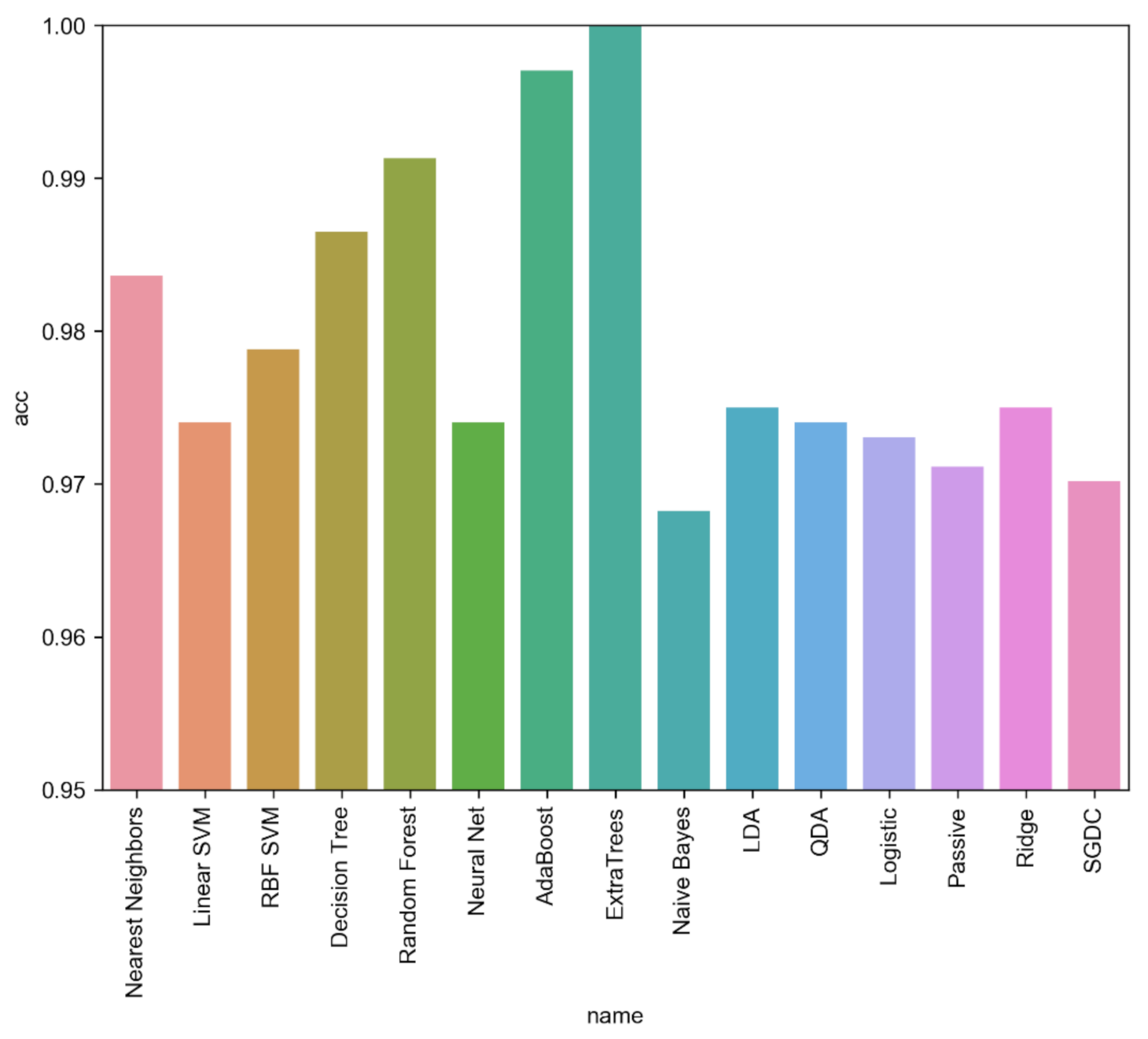
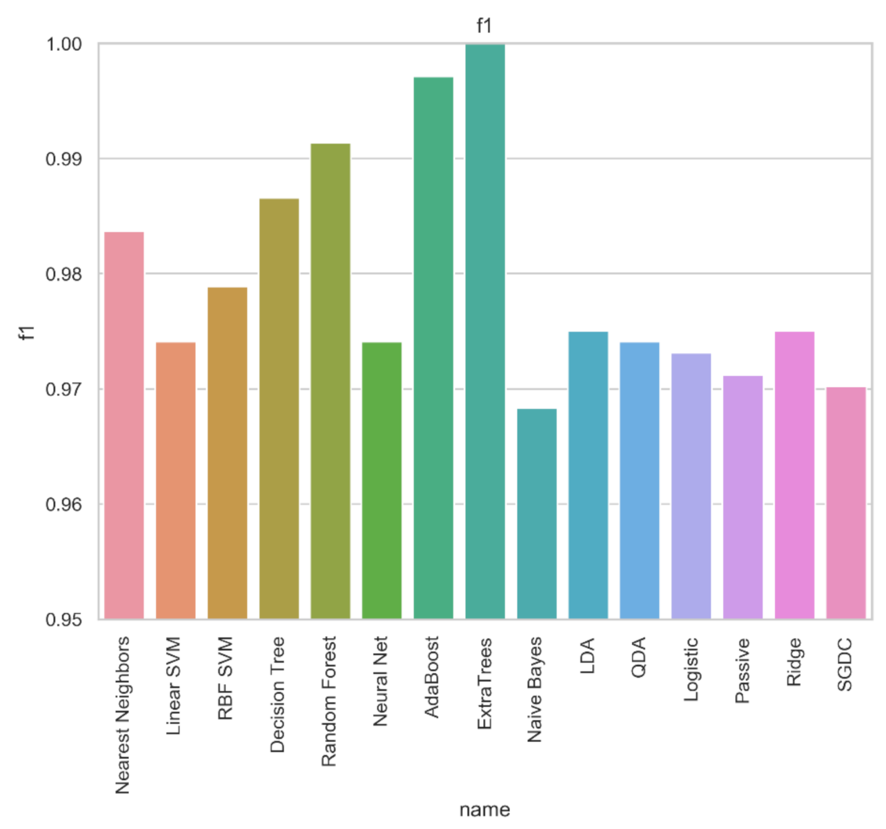
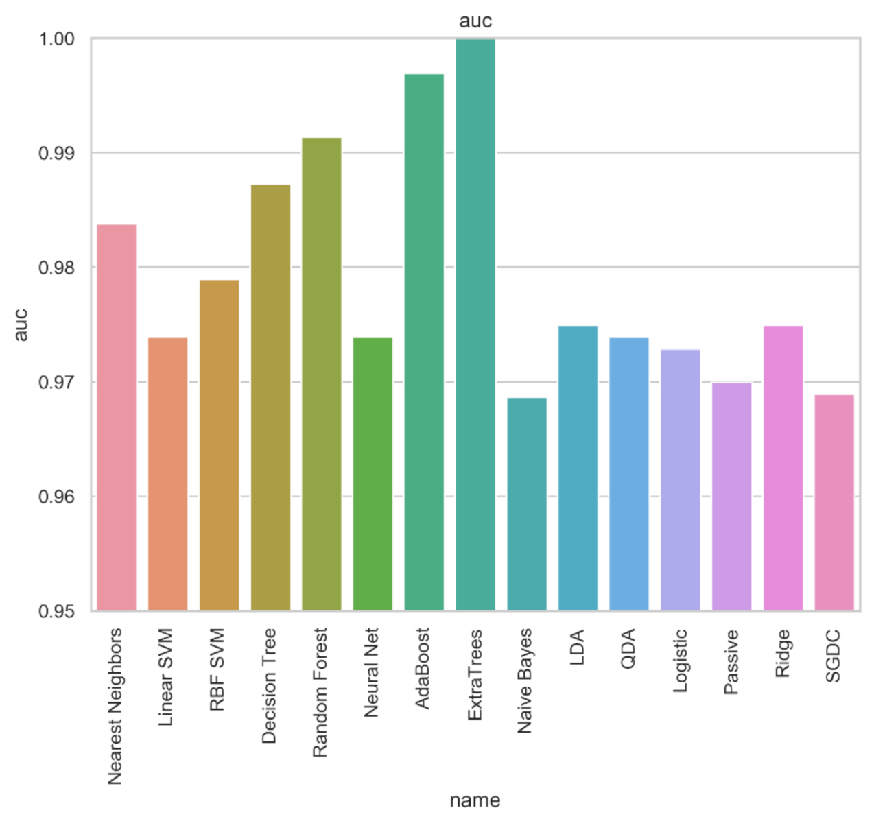
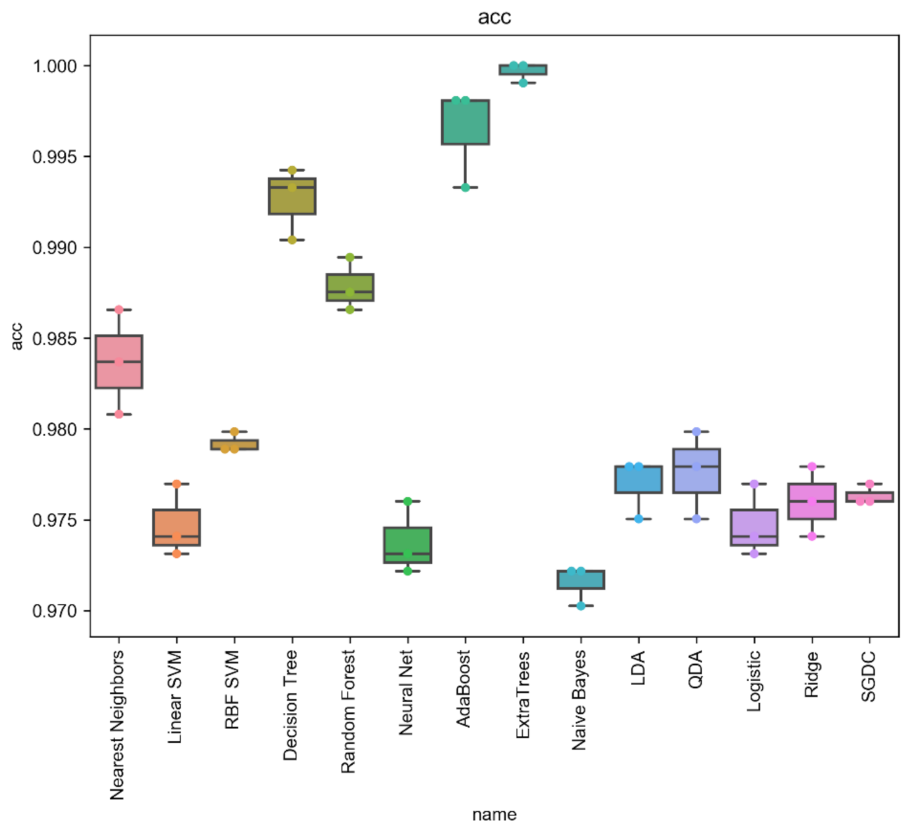
| Meta-Learner | Acc | Prec | Rec | Spec | FPR | FNR | F1 | AUC | MCC | Kappa |
|---|---|---|---|---|---|---|---|---|---|---|
| Nearest Neighbors | 0.984 | 0.984 | 0.984 | 0.984 | 0.014 | 0.018 | 0.984 | 0.984 | 0.967 | 0.967 |
| Linear SVM | 0.974 | 0.974 | 0.974 | 0.974 | 0.029 | 0.023 | 0.974 | 0.974 | 0.948 | 0.948 |
| RBF SVM | 0.979 | 0.979 | 0.979 | 0.979 | 0.021 | 0.022 | 0.979 | 0.979 | 0.958 | 0.958 |
| Decision Tree | 0.987 | 0.987 | 0.987 | 0.987 | 0.002 | 0.023 | 0.987 | 0.987 | 0.973 | 0.973 |
| Random Forest | 0.991 | 0.991 | 0.991 | 0.991 | 0.008 | 0.009 | 0.991 | 0.991 | 0.983 | 0.983 |
| Neural Net | 0.974 | 0.974 | 0.974 | 0.974 | 0.029 | 0.023 | 0.974 | 0.974 | 0.948 | 0.948 |
| AdaBoost | 0.997 | 0.997 | 0.997 | 0.997 | 0.006 | 0 | 0.997 | 0.997 | 0.994 | 0.994 |
| ExtraTrees | 0.999 | 0.999 | 0.998 | 1.000 | 0.000 | 0.002 | 0.999 | 0.999 | 0.999 | 0.999 |
| Naive Bayes | 0.968 | 0.968 | 0.968 | 0.968 | 0.027 | 0.036 | 0.968 | 0.969 | 0.937 | 0.936 |
| LDA | 0.975 | 0.975 | 0.975 | 0.975 | 0.027 | 0.023 | 0.975 | 0.975 | 0.95 | 0.95 |
| QDA | 0.974 | 0.974 | 0.974 | 0.974 | 0.029 | 0.023 | 0.974 | 0.974 | 0.948 | 0.948 |
| Logistic | 0.973 | 0.973 | 0.973 | 0.973 | 0.031 | 0.023 | 0.973 | 0.973 | 0.946 | 0.946 |
| Ridge | 0.971 | 0.971 | 0.971 | 0.971 | 0.049 | 0.011 | 0.971 | 0.97 | 0.943 | 0.942 |
| SGDC | 0.975 | 0.975 | 0.975 | 0.975 | 0.027 | 0.023 | 0.975 | 0.975 | 0.95 | 0.95 |
| Case | Acc | Prec | Rec | Spec | FPR | FNR | F1 | AUC | MCC | Kappa |
|---|---|---|---|---|---|---|---|---|---|---|
| ENSEMBLE1 | 0.989 | 0.988 | 0.987 | 0.979 | 0.011 | 0.012 | 0.989 | 0.989 | 0.968 | 0.968 |
| ENSEMBLE2 | 0.985 | 0.983 | 0.985 | 0.983 | 0.017 | 0.014 | 0.984 | 0.984 | 0.967 | 0.967 |
| ENSEMBLE3 | 0.985 | 0.984 | 0.984 | 0.985 | 0.013 | 0.016 | 0.986 | 0.988 | 0.971 | 0.970 |
| Full Model | 0.999 | 0.999 | 0.998 | 1.000 | 0.000 | 0.002 | 0.999 | 0.999 | 0.999 | 0.999 |
Publisher’s Note: MDPI stays neutral with regard to jurisdictional claims in published maps and institutional affiliations. |
© 2021 by the authors. Licensee MDPI, Basel, Switzerland. This article is an open access article distributed under the terms and conditions of the Creative Commons Attribution (CC BY) license (http://creativecommons.org/licenses/by/4.0/).
Share and Cite
Damaševičius, R.; Venčkauskas, A.; Toldinas, J.; Grigaliūnas, Š. Ensemble-Based Classification Using Neural Networks and Machine Learning Models for Windows PE Malware Detection. Electronics 2021, 10, 485. https://doi.org/10.3390/electronics10040485
Damaševičius R, Venčkauskas A, Toldinas J, Grigaliūnas Š. Ensemble-Based Classification Using Neural Networks and Machine Learning Models for Windows PE Malware Detection. Electronics. 2021; 10(4):485. https://doi.org/10.3390/electronics10040485
Chicago/Turabian StyleDamaševičius, Robertas, Algimantas Venčkauskas, Jevgenijus Toldinas, and Šarūnas Grigaliūnas. 2021. "Ensemble-Based Classification Using Neural Networks and Machine Learning Models for Windows PE Malware Detection" Electronics 10, no. 4: 485. https://doi.org/10.3390/electronics10040485