Identification of Plant-Leaf Diseases Using CNN and Transfer-Learning Approach

Abstract

The timely identification and early prevention of crop diseases are essential for improving production. In this paper, deep convolutional-neural-network (CNN) models are implemented to identify and diagnose diseases in plants from their leaves, since CNNs have achieved impressive results in the field of machine vision. Standard CNN models require a large number of parameters and higher computation cost. In this paper, we replaced standard convolution with depth=separable convolution, which reduces the parameter number and computation cost. The implemented models were trained with an open dataset consisting of 14 different plant species, and 38 different categorical disease classes and healthy plant leaves. To evaluate the performance of the models, different parameters such as batch size, dropout, and different numbers of epochs were incorporated. The implemented models achieved a disease-classification accuracy rates of 98.42%, 99.11%, 97.02%, and 99.56% using InceptionV3, InceptionResNetV2, MobileNetV2, and EfficientNetB0, respectively, which were greater than that of traditional handcrafted-feature-based approaches. In comparison with other deep-learning models, the implemented model achieved better performance in terms of accuracy and it required less training time. Moreover, the MobileNetV2 architecture is compatible with mobile devices using the optimized parameter. The accuracy results in the identification of diseases showed that the deep CNN model is promising and can greatly impact the efficient identification of the diseases, and may have potential in the detection of diseases in real-time agricultural systems.

1. Introduction

The automated identification of plant diseases based on plant leaves is a major landmark in the field of agriculture. Moreover, the early and timely identification of plant diseases positively impacts crop yield and quality [1]. Due to the cultivation of a large number of crop products, even an agriculturist and pathologist may often fail to identify the diseases in plants by visualizing disease-affected leaves. However, in the rural areas of developing countries, visual observation is still the primary approach of disease identification [2]. It also requires continuous monitoring by experts. In remote areas, farmers may need to travel far to consult an expert, which is time-consuming and expensive [3,4]. Automated computational systems for the detection and diagnosis of plant diseases assist farmers and agronomists with their high throughput and precision.

In order to overcome the above problems, researchers have thought of several solutions. Various types of feature sets can be used in machine learning for the classification of plant diseases. Among these, the most popular feature sets are traditional handcrafted and deep-learning (DL)-based features. Preprocessing, such as image enhancement, color transformation, and segmentation [5], is a prerequisite before efficiently extracting features. After feature extraction, different classifiers can be used. Some popular classifiers are K-nearest neighbor (KNN) [6], support vector machine (SVM) [7], decision tree, random forest (RF) [8], naive Bayes (NB), logistic regression (LR), rule generation [9], artificial neural networks (ANNs), and Deep CNN. KNN is a simple supervised-machine-learning algorithm used in classification problems, and it uses similarity measurements (i.e., distance, proximity, or closeness) [10]. SVM is also a popular supervised-machine-learning technique used for classification purposes [11,12]. The idea behind SVM is to find a hyperplane between data classes that divides each class [13,14]. An NB classifier makes predictions on the basis of probability measurements [15]. It assumes that the generated features are independent from each other [16]. ANN is a set of connected inputs, an output network that is modeled after the human neural system cells [17]. The network consists of an input layer, intermediate layer, and output layer. Learning is performed by adjusting weights [18]. Handcrafted-feature-based methods achieve good classification results, but have some limitations such as requiring huge amounts of preprocessing, and the process is time-consuming. Feature extraction in the handcrafted-based approach is limited, and extracted features might not be enough for correct identification, which affects accuracy.

On the other hand, deep-learning-based techniques, particularly CNNs, are the most promising approach for automatically learning decisive and discriminative features. Deep learning (DL) consists of different convolutional layers that represent learning features from the data [19,20]. Plant-disease detection can be accomplished using a deep-learning model [21,22,23]. Deep learning also has some drawbacks, as it requires large amounts of data to train the network. If an available dataset does not contain enough images, performance is worse. Transfer learning has several advantages; for example, it does not needs a large amount of data to train the network. Transfer learning improves learning a new task through knowledge transfer from a similar task that had already been learned. Many studies used transfer learning in their disease-detection approach [24,25,26,27]. The benefits of using transfer learning are a decrease in training time, generalization error, and computational cost of building a DL model [28]. In this work, we use different DL models to identify plant diseases. The inception module can extract more specific and relevant features as it allows for simultaneous multilevel feature extraction. We replaced the standard convolution of an inception block with depthwise separable convolution to reduce the parameter number. Multiple feature extraction improves the performance of the model. In a residual network, it has a shortcut connection that basically feeds the previous layer output to the next layer, which strengthens features and improves accuracy. To evaluate performance on a lightweight memory-efficient interface, the MobileNet model is used. MobileNetV2 architecture can achieve high accuracy rates while keeping parameter number and computation as low as possible. According to [29], network depth, width, and resolution can lead to better performance accuracy with fewer parameters. We also used this EfficientNet model to identify diseases in plant and evaluated its performance. In the implemented DL architecture, we used different batch sizes of 32–180 to evaluate performance. Different dropout values and learning rates were also used to examine performance. Several epochs were used to run the model. The evaluation showed that the implemented deep CNN achieved impressive results and better performance in comparison with those of state-of-the-art machine-learning techniques.The main contributions of the paper are as follows:

• Different convolutional-neural-network (CNN) architectures such as InceptionV3, InceptionResNetV2, MobileNetV2, and EfficientNetB0 are implemented to diagnose plant diseases on the basis of healthy- and diseased-leaf images.
• In InceptionV3 and InceptionResNetV2, standard convolution was replaced with depthwise separable convolution, which reduced the number of parameters by a large margin while achieving the same performance-accuracy level.
• The implemented InceptionV3 and InceptionResNetV2 use fewer parameters and are faster than the standard InceptionV3 and InceptionResNetV2 architectures.
• A transfer-learning-based CNN was applied on a MobileNetV2 and an EfficientNetB0 model. In each model, we froze the layer weight before the fully connected layer and removed all layers after that. We added a stack of an activation layer, batch-normalization layer, and dense layer. After each batch-normalization layer, we used a dropout layer with different dropout values, which prevents the architecture from overfitting. Since a large number of features were there, we used the L1 and L2 regularization techniques in the dense layer of all models, which simplified the models.
• We finetuned the network with different parameters to achieve optimal results. We performed extensive testing by adjusting the different parameters. We used different batch sizes in the range of 32–180, and different dropout values in the range of 0.2–0.8. To optimize the model, we tested it with different learning rates in the range of 0.01–0.0001. The models were trained with different epochs.
• To examine the robustness of the model, we used three formats of images, namely, color, segmented, and grayscale images.
• We compared the performance of the implemented models with that of other deep-learning models and state-of-the-art machine-learning techniques. Results showed that the implemented model performed better in terms of both accuracy and required training time.

This paper is organized as follows. Section 2 illustrates the literature related to the detection of plant diseases. Section 3 presents the CNN models and the details of the datasets that are used in the experiments, along with their class and labels. Section 4 presents the results and performance of the models on the basis of their ability to predict the correct class among 38 different classes. Section 5 offers a discussion, and outlines the study’s limitations and future directions towards the development and enhancement of the system Section 6 concludes the work.

2. Related Work

The implementation of proper techniques to identify healthy and diseased leaves helps in controlling crop loss and increasing productivity. This section comprises different existing machine-learning techniques for the identification of plant diseases.

2.1. Shape- and Texture-Based Identification

In [30], the authors identified diseases using tomato-leaf images. They used different geometric and histogram-based features from segmented diseased portions and applied an SVM classifier with different kernels for classification. S.Kaur et al. [31] identified three different soybean diseases using different color and texture features. In [32] P Babu et al. used a feed-forward neural network and backpropagation to identify plant leaves and their diseases. S. S. Chouhan et al. [33] used a bacterial-foraging-optimization-based radial-basis-function neural network (BRBFNN) for the identification of leaves and fungal diseases in plants. In their approaches, they used a region-growing algorithm to extract features from a leaf on the basis of seed points having similar attributes. The bacterial-foraging optimization technique is used to speed up a network and improve classification accuracy.

2.2. Deep-Learning-Based Identification

Mohanty et al. [24] used AlexNet and GoogleNet CNN architectures in the identification of 26 different plant diseases. Ferentinos et al. [25] used different CNN architectures to identify 58 different plant diseases, achieving high levels of classification accuracy. In their approach, they also tested the CNN architecture with real-time images. Sladojevic et al. [26] designed a DL architecture to identify 13 different plant diseases. They used the Caffe DL framework to perform CNN training. Kamilaris et al. [34] exhaustively researched different DL approaches and their drawbacks in the field of agriculture. In [35], the authors proposed a nine-layer CNN model to identify plant diseases. For experimentation purposes, they used the PlantVillage dataset and data-augmentation techniques to increase the data size, and analyzed performance. The authors reported better accuracy than that of a traditional machine-learning-based approach.

Pretrained AlexNet and GoogleNet were used in [36] to detect 3 different soybean diseases from healthy-leaf images with modified hyperparameters such as minibatch size, max epoch, and bias learning rate. Six different pre-trained network(AlexNet, VGG16, VGG19, GoogLeNet, ResNet101 and DenseNet201) used by KR Aravind et al. [37] to identify 10 different diseases in plants, and they achieved the highest accuracy rate of 97.3% using GoogleNet. A pretrained VGG16 as the feature extractor and multiclass SVM were used in [38] to classify different eggplant diseases. Different color spaces (RGB, HSV, YCbCr, and grayscale) were used to evaluate performance; using RGB images, the highest classification accuracy of 99.4% was achieved. In [39], the authors classified maize-leaf diseases from healthy leaves using deep-forest techniques. In their approach, they varied the deep-forest hyperparameters regarding number of trees, forests, and grains, and compared their results with those of traditional machine-learning models such as SVM, RF, LR, and KNN. Lee et al. compared different deep-learning architectures in the identification of plant diseases [22]. To improve the accuracy of the model, Ghazi et al. used a transfer-learning-based approach on pretrained deep-learning models [40].

In [41], the authors used a shallow CNN with SVM and RF classifiers to classify three different types of plant diseases. In their work, they mainly compared their results with those of deep-learning methods and showed that classification using SVM and RF classifiers with extracted features from the shallow CNN outperformed pretrained deep-learning models. A self-attention convolutional neural network (SACNN) was used in [42] to identify several crop diseases. To examine the robustness of the model, the authors added different noise levels in the test-image set.

Oyewola et al. [43] identified 5 different cassava-plant diseases using plain convolutional neural network (PCNN) and deep residual network (DRNN), and found that DRNN outperformed PCNN by a margin of 9.25%. Ramacharan et al. [4] used a transfer-learning approach in the identification of three diseases and two pest-damage types in cassava plants. The authors then extended their work on the identification of cassava plant diseases using a smartphone-based CNN model and achieved accuracy of 80.6% [44].

A NASNet-based deep CNN architecture was used in [45] to identify leaf diseases in plants, and an accuracy rate of 93.82% was achieved. Rice- and maize-leaf diseases were identified by Chen et al. [2] using the INC-VGGN method. In their approach, they replaced the last convolutional layer of VGG19 with two inception layers and one global average pooling layer. A shallow CNN (SCNN) was used by Yang Li et al. [41] in the identification of maize, apple, and grape diseases. First, they extracted CNN features and classified them using SVM and RF classifiers. Sethy et al. [1] used different deep-learning models to extract features and classify them using an SVM classifier. Using ResNet50 with SVM, they achieved the highest performance accuracy. A VGG16, ResNet, and DenseNet model was used by Yafeng Zhao et al. [46] to identify plant diseases from the plant village dataset. To increase the dataset size, they used a double generative adversarial network (DoubleGAN), which improved the performance results. A summary of the related work on plant-disease identification based on leaf images is shown in

Table 1. Summary of related work on plant-disease detection.

Author	Methods	Results
Mohantyet al. [24] (2016)	AlexNet and GoogleNet	99.27% in AlexNet 99.34% in GoogleNet
Sladojevic et al. [26] (2016)	Finetuned CNN architecture	96.3% accuracy
Ramcharan et al. [4] (2017)	Inception V3 based on GoogleNet	93% accuracy
Fuentes et al. [23] (2017)	Faster R-CNN	83% accuracy
Ferentinos et al. [25] (2018)	AlexNetOWTBn and VGG	99.49% in AleXNetOWTBn 99.53% in VGG
Ramacharan el al. [44] (2019)	Single-shot multibox (SSD) model with MobileNet detector and classifier	80.6% accuracy on images 70.4% accuracy on video
Geetharamani et al. [35] (2019)	Nine-layer deep CNN	96.46% accuracy
Chen et al. [2] (2020)	INC VGGN	92% accuracy
Li et al. [41] (2020)	Shallow CNN with SVM and RF	94% accuracy
Oyewola et al. [43] (2021)	Deep residual neural network (DRNN)	96.75% accuracy

.

3. Materials and Methods

3.1. Convolutional-Neural-Network Models

Interest in CNNs has recently surged, and DL is the most popular architecture because DL models can learn relevant features from input images at different convolutional levels similar, to the function of the human brain. DL can solve complex problems particularly well and quickly with high classification accuracy and a lower error rate [47]. The DL model is composed of different components (convolutional, pooling layer, and fully connected layers, and activation functions).

Table 2. Comparison among different CNN architectures regarding layer number and parameter size.

Model	No. of Layer	Parameters (Million)	Size
AlexNet	8	60	-
VGGNet-16	23	138	528 MB
VGGNet-19	26	143	549 MB
Inception-V1	27	7	-
Inception-V3	42	27	93 MB
ResNet-152	152	50	132 MB
ResNet-101	101	44	171 MB
InceptionResNetV2	572	55	215 MB
MobileNet-V1	28	4.2	16 MB
MobileNet-V2	28	3.37	14 MB
EfficientNet B0	-	5	-

shows the number of layers and parameter sizes of different CNN architectures. AlexNet has a layer size of 8 and 60 millions parameters, whereas VGGNet-16 and GoogleNet have parameter sizes of 138 and 7 million, respectively. The layers in those two models are 16 and 27. The layers in ResNet-152 are 152, and the parameter size is 50 million. InceptionV3, MobileNetV1, and MobileNetV2 have a parameter size of 27, 4.2, and 3.37 million, respectively. In our work, we used the InceptionV3, InceptionResNetV2, MobileNetV2, and EfficientNetB0 architectures to identify different plant diseases using the leaves of different disease-affected plants. We used these models because their parameter size is optimal in comparison with that of other architectures. During implementation, we used a pretrained weight based on the ImageNet Large-Scale Visual Recognition (ILSVRC) [48] dataset.

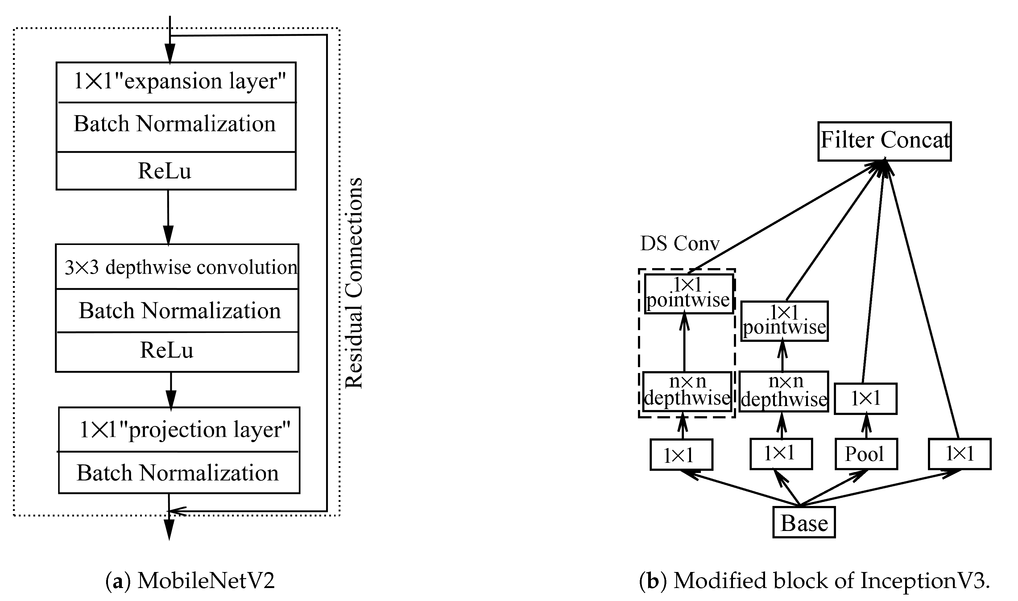
Convolutional neural networks became familiar in machine vision since the AlexNet model was popularized in DL architecture. The development of the Inception model was important in the field of machine vision. Inception is a simple and more powerful DL network with sparsely connected filters, which can replace fully connected network architectures, especially inside convolutional layers, as shown in Figure 1b. The Inception model’s computational efficiency and number of used parameters are much lower in comparison with those of other models such as AlexNet and VGGNet. An inception layer consists of differently dized convolutional layers (e.g., 1 × 1, 3 × 3, and n × n convolutional layers) and pooling layers with all outputs integrated together and propagating to the input of the next layer. Instead of using standard convolution in the inception block, we used depthwise separable convolution.

Table 3. Required parameters using standard convolution in the Inception block.

Layer	Input	Filter (Size/Number)	Parameter
Input image	299 × 299 × 3	-	-
Conv1	Input image	1 × 1/32	128
Conv2	Conv1	1 × 1/64	2112
Conv3	Conv1	1 × 1/64	2112
Conv4	Conv3	3 × 3/96	55,392
Conv5	Conv1	1 × 1/64	2112
Conv6	Conv5	5 × 5/48	76,848
Avg. pooling	Conv1	3 × 3	-
Conv7	Avg. pooling	1 × 1/32	1056
Total			139,760

and

Table 4. Required parameters using depthwise separable convolution in the Inception block.

Layer	Input	Filter (Size/Number)	Parameter
Input image	299 × 299 × 3	-	-
Conv1	Input image	1 × 1/32	128
Conv2	Conv1	1 × 1/64	2112
Conv3	Conv1	1 × 1/64	2112
Depthwise separable conv1	Conv3	3 × 3/96	6816
Conv4	Conv1	1 × 1/64	2112
Depthwise separable conv2	Conv4	5 × 5/48	4720
Avg. pooling	Conv1	3 × 3	-
Conv5	Avg. pooling	1 × 1/32	1056
Total			19,056

show the required parameters in standard convolution and depthwise separable convolution, respectively. The number of parameters required in depthwise separable convolution is much less than that of standard convolution.

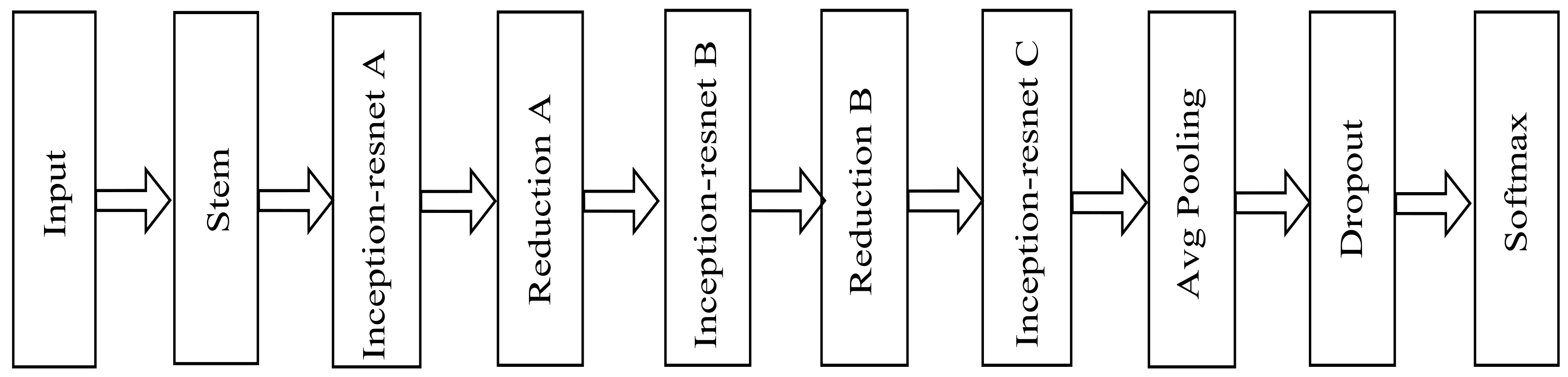
The InceptionResNetV2 architecture is the combination of recent deep-learning models: residual connection and the Inception architecture [49]. This hybrid deep-learning model has the advantages of a residual network and retains the unique characteristics of the multiconvolutional core of the Inception network. In [50], the authors showed that residual connections are implicit approaches for training very deep architectures. This improved version of the Inception architecture significantly improved performance and accelerated the model. Figure 2 shows the basic block diagram of InceptionResNetV2.

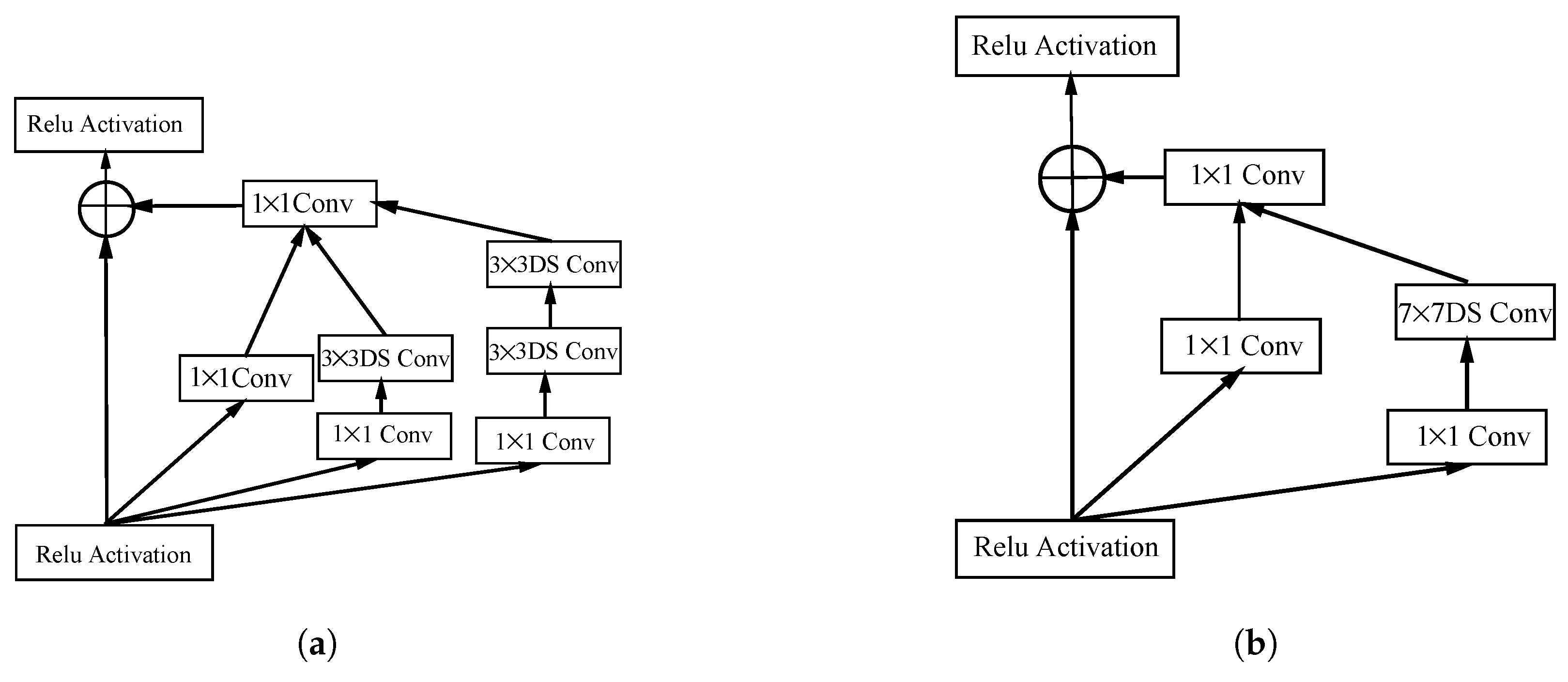
InceptionResNetV2 consists of three inception blocks. Figure 3a shows the modified InceptionResNet-A block where the inception module uses parallel structure to extract the features. The 3 × 3 standard convolution was replaced by 3 × 3 depthwise separable convolution. Figure 3b represents the modified InceptionResNet-B block, where the 7 × 7 standard convolutional structure of inception model was replaced by 7 × 7 depthwise separable convolution.

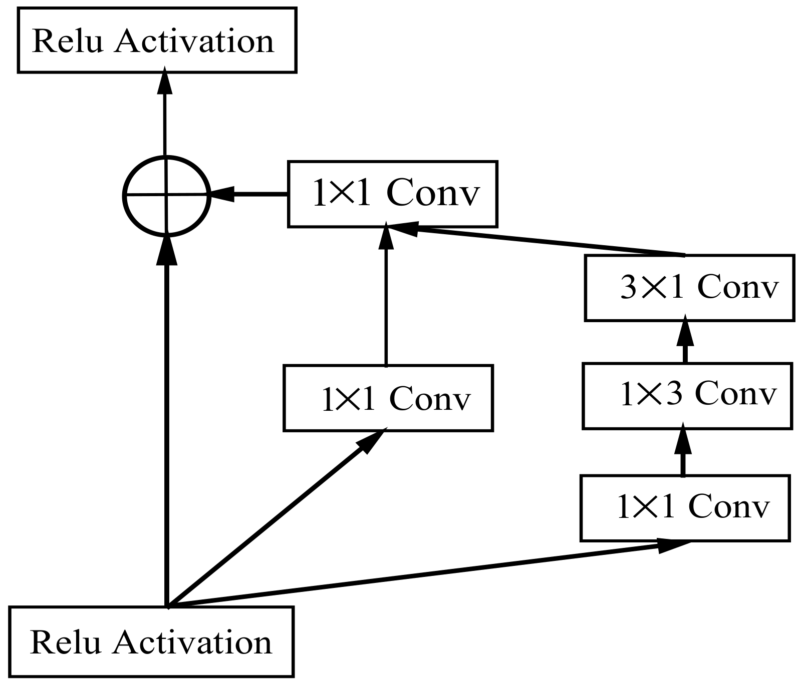
In the InceptionResNet-C block, the 3 × 3 convolutional structure was replaced by successive 3 × 1 and 1 × 3, as shown in Figure 4. By replacing the original convolutional kernel with multiple smaller convolutional kernels, this model effectively reduced computational complexity. An increase in the number of convolutional layers and the deepening of the network improved performance accuracy.

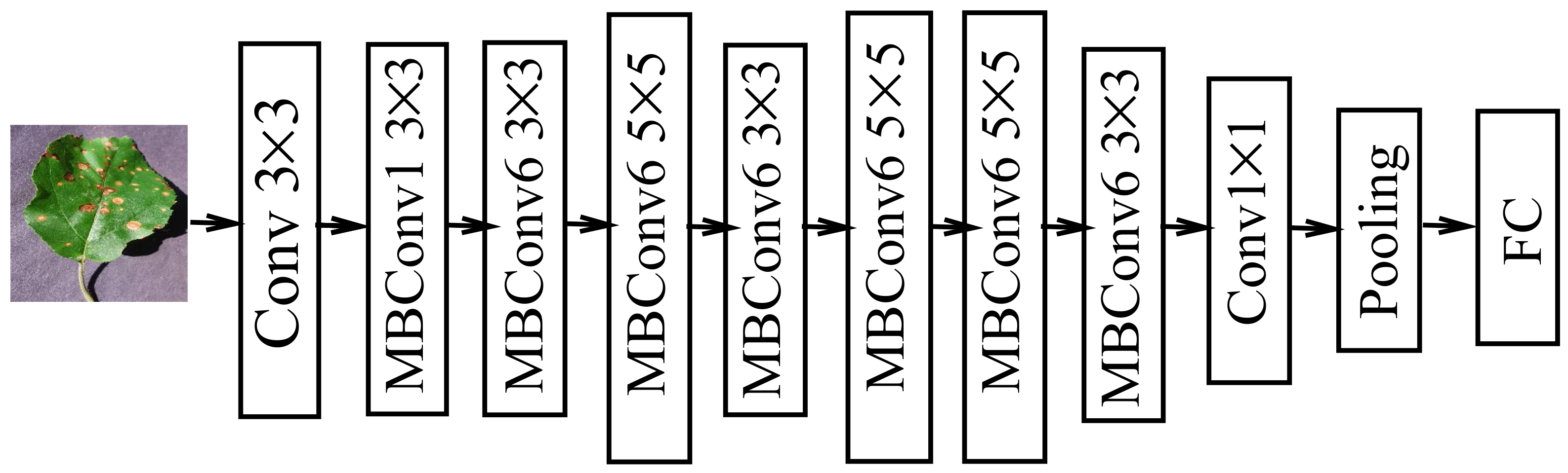
The main intention behind the use of MobileNetV2 architecture is the convolutional layer, which is quite expensive in normal convolutions in comparison with in MobileNetV2. To improve efficiency, depthwise separable convolution is used in the MobileNetV2 architecture [51,52]. Depthwise convolution is independently performed for each input channel. The blocks of MobileNetV2 are shown in Figure 1a. The first layer is called the expansion layer of 1 × 1 convolution, and its purpose is to expand the number of channels in the data. Next is the projection layer. In this layer, a high number of dimensions is reduced to a smaller number. Except for the projection layer, each layer comprises a batch-normalization function and activation function ReLU. In the MobileNetV2 architecture, there is one residual connection between input and output layers. The residual network tries to learn already learned features; those that are not useful in decision making are discarded. This architecture can reduce the number of computations and of parameters. The MobileNetV2 architecture consists of 17 building blocks in a row followed by a 1 × 1 convolutional layer, global average pooling layer, and classification layer.

A deep-learning architecture aims to achieve better performance accuracy and efficiency with smaller models. Unlike other state-of-the-art deep=learning models, the EfficientNet architecture is a compound scaling method that uses a compound coefficient to uniformly scale network width, depth, and resolution [29]. EfficientNet consists of 8 different models from B0 to B7. Instead of using the ReLU activation function, EfficientNet uses a new activation function, swish activation. EfficientNet uses inverted bottleneck convolution, which was first introduced in the MobileNetV2 model, which consists of a layer that first expands the network and then compresses the channels [52]. This architecture reduces computation by a factor of $f^2$ as compared to normal convolution, where f is the filter size. The authors in [29] showed that EfficientNetB0 is the simplest of all 8 models and uses fewer parameters. So, in our experiment, we directly used EfficientNetB0 to evaluate performance. Figure 5 shows the basic block diagram of EfficientNetB0.

3.2. Transfer-Learning Approach

In deep learning, transfer learning is the reuse of a pretrained network on a new task. Transfer learning is very popular in deep learning because it can train the network with a small amount of data and high accuracy. In transfer learning, a machine exploits knowledge gained from a previous task to improve generalization about another. In transfer learning, the last few layers of the trained network are replaced with new layers, such as a fully connected layer and softmax classification layer, with number of classes, which is 38 in our paper. In each model, we unfroze the layer and added a stack of one activation layer, one batch-normalization layer, and one dropout layer. All models were tested with different dropout values, learning rates, and batch sizes. The input size used in MobileNetV2 and EfficientnetB0 is 224 × 224.

3.3. Dataset

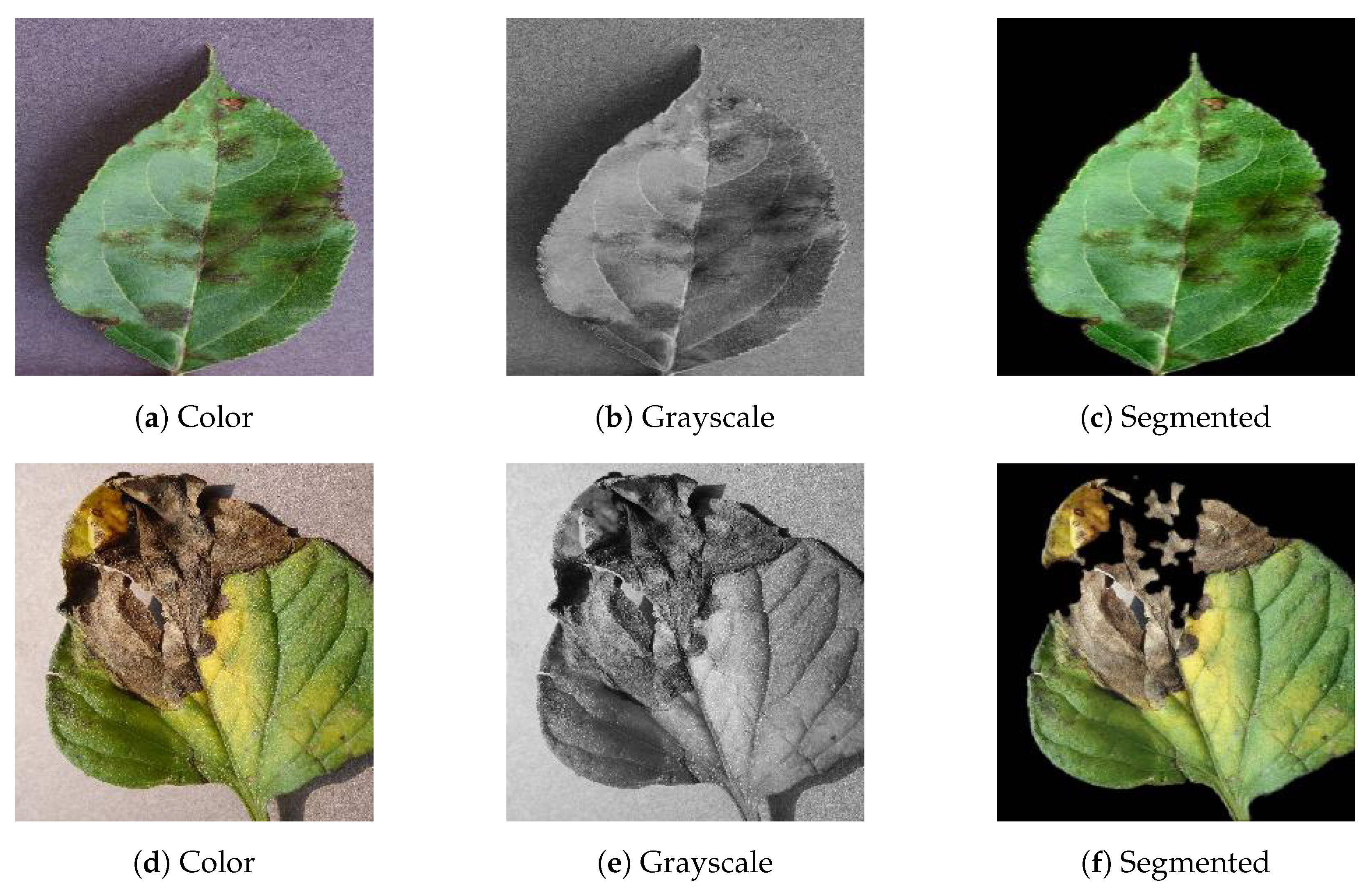
For training and testing purposes, we used the standard open-access PlantVillage dataset [53], which consists of 54,305 numbers of healthy- and infected-plant leaves. Detailed database information, the number of classes and images in each class, their common and scientific names, and the disease-causing viruses are shown in

Table 5. Detailed description of PlantVillage dataset with relative information.

Class	Plant Name	Disease Name	Causes Virus Name	Type of Disease	No. of Images
C1	Apple	Healthy	-	-	1645
C2	Apple	Apple scab	Venturiainaequalis	Fungus	630
C3	Apple	Black rot	Botryosphaeriaobtusa	Fungus	621
C4	Apple	Cedar apple rust	Gymnosp-orangium	Fungus	275
C5	Blueberry	Healthy	-	-	1502
C6	Cherry	Healthy	-	-	854
C7	Cherry	Powdery mildew	Podosphaeraclandestina	Biotrophic Fungus	1052
C8	Corn	Healthy	-	-	1162
C9	Corn	Cercospora leaf spot	Cercosporazeae-maydis	Fungal	513
C10	Corn	Common rust	Puccinia sorghi	Fungus	1192
C11	Corn	Northern Leaf Blight	Exserohilumturcicum	Foliar	985
C12	Grape	Healthy	-	-	423
C13	Grape	Black rot	Guignardiabidwellii	Fungus	1180
C14	Grape	Esca (Black Measles)	Phaeomoniellachlamydospora	Fungus	1383
C15	Grape	Leaf blight (Isariopsis)	Pseudocercosporavitis	Fungus	1076
C16	Orange	Healthy	-	-	5507
C17	Peach	Healthy	-	-	360
C18	Peach	Bacterial spot	Xanthomonascampestris pv. pruni	Bacterial	2297
C19	Pepper/bell	Healthy	-	-	1478
C20	Pepper/bell	Bacterial spot	Xanthomonascampestris pv.	Bacterial	997
C21	Potato	Healthy	-	-	152
C22	Potato	Early blight	Alternaria solani	Fungal	1000
C23	Potato	Late blight	Phytophthorainfestans	Fungal	1000
C24	Raspberry	Healthy	-	-	371
C25	Soybean	Healthy	-	-	5090
C26	Squash	Powdery mildew	Podosphaeraxanthii	Fungal	1835

and

Table 6. Detailed description of PlantVillage Dataset with relative information.

Class	Plant Name	Disease Name	Causes Virus Name	Type of Disease	No. of Images
C27	Strawberry	Healthy	-	-	456
C28	Strawberry	Leaf scorch	Diplocarpon earliana	Fungal	1109
C29	Tomato	Healthy	-	-	1591
C30	Tomato	Bacterial spot	Xanthomonas perforans	Bacterial	2127
C31	Tomato	Early blight	Alternaria˙sp.	Fungal	1000
C32	Tomato	Late blight	Phytophthora infestans	Fungal	1909
C33	Tomato	Leaf Mold	Lycopersicon	Fungal	952
C34	Tomato	Septoria leaf spot	Septoria lycopersici	Fungal	1771
C35	Tomato	Spider mites	Tetranychus spp.	Pest	1676
C36	Tomato	Target Spot	Corynespora cassiicola	Fungal	1404
C37	Tomato	Tomato mosaic virus	Tomato mosaic	Viral	373
C38	Tomato	Tomato Yellow Leaf	Begomovirus	Viral	5357

. The database contains 38 different classes of 14 different plant species with healthy- and disease-affected-leaf images. All images were captured in laboratory conditions. Figure 6 shows some sample leaf images from the PlantVillage datasets [53].

In our experiment, we used three different formats of PlantVillage datasets. First, we ran the experiment with colored leaf images, and then with segmented leaf images of the same dataset. In the segmented images, the background was smoothed, so that it could provide more meaningful information that would be easier to analyze. Lastly, we used grayscale images of the same dataset to evaluate the performance of the implemented methods. All leaf images were divided into two sets, a training set and the testing set. To evaluate performance, we split leaf images into three different sets, namely 80–20 (80% training images and 20% testing images), 70–30 (70% training images and 30% testing images), and 60–40 (60% training images and 40% testing images).

4. Results

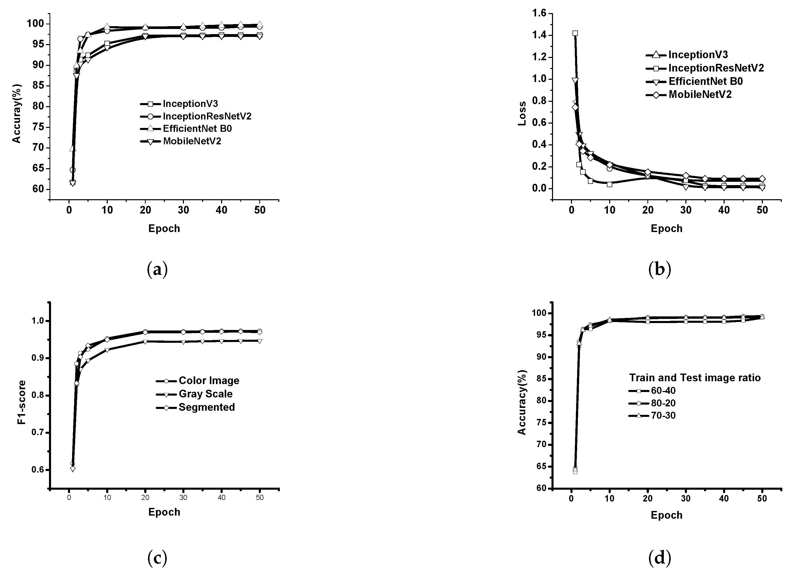
The implemented CNN architectures, as described in the previous section, used the parameters in

Table 7. Parameters used in CNN for training.

Parameters	Value
Training epoch	30–50
Batch size	32–180
Dropout	0.2–0.8
Learning rate	0.01–0.0001

. EfficientNetB0 achieved the best accuracy in comparison with that of InceptionV3, MobileNetV2, and InceptionResNetV2. To evaluate performance, we used different parameters, for example, performance accuracy, F1 score, precision, recall, training loss, and time required per epoch. As in our experiment, we used three different representations (i.e., color, grayscale, segmented) of PlantVillage image data, which showed different performance metrics in all cases. The color-image dataset performed better than those with grayscale and segmented images; the same number of CNN network parameters was maintained in all cases. Figure 7a–c shows the graphs for testing the accuracy, loss, and F1-score regarding the number of epochs for the implemented models. Figure 7d represents the accuracy graph of the InceptionResnetV2 model with different training and testing split images. A summary of the performance comparisons of the implemented models based on testing accuracy and testing loss is represented in

Table 8. Performance comparison of different DL architectures.

Model	Training Acc (%)	Testing Acc (%)	Loss	Epoch	Avg Time (s/Epoch)
AlexNet [25]	-	98.64	0.0658	50	7034
VGG [25]	-	98.87	0.0542	49	4208
NASNet [45]	-	93.82	-	9	-
ResNet	-	92.56	-	-	-
Deep CNN [26]	-	96.3	-	100,000	-
Nine Layer CNN [35]	97.87	96.46	0.2487	3000	-
CNN [54]	99.99	97.1	-	-	-
InceptionV3	98.92	98.42	0.0129	50	1027
InceptionResNetV2	99.47	99.11	0.0241	50	836
MobileNetV2	97.17	97.02	0.0921	50	565
EfficientNetB0	99.78	99.56	0.0091	50	545

. The performance metrics that are considered in our proposed work are as follows.

• Performance accuracy: the total number of correctly classified images to the total number of images.
• Loss function: how well the architecture models the data.
• Precision: the ratio of the number of correctly predicted observations (true positives) to the total number of positive predictions (true positives + false positives).
• Recall: the ratio of correctly predicted observations (true positives) to all observations in that class (true positives + false negatives).
• F1 score: the harmonic mean between precision and recall.
• Time requirement (in sec) per epoch for training each DL model.

To avoid overfitting, we phasewise divided the dataset into different training and testing ratios. In the case of 80% of training and 20% of testing image data, we achieved an accuracy of 98.42% in InceptionV3, 99.11% in InceptionResNetV2, 97.02% in MobilenetV2, and 99.56% in EfficientNetB0 for color images. After splitting the dataset into different training and testing ratios, there was not much variation in the accuracy of the models. Hence, they did not suffer from the problem of overfitting.The accuracy of all models for different image types with loss and number of epochs are shown in

Table 9. Accuracy and loss of implemented models regarding different image types along with different train-test split ratios.

Dataset	Model	Image Type	Accuracy(%)	Loss	Epoch
Train-80% Test-20%	InceptionV3	Color	98.92	0.0392	50
		Grayscale	96.39	0.1391	50
		Segmented	98.71	0.0571	50
	InceptionResNetV2	Color	99.47	0.0731	50
		Grayscale	98.13	0.0972	50
		Segmented	99.39	0.0347	50
	MobileNetV2	Color	97.17	0.0921	50
		Grayscale	93.53	0.1152	50
		Segmented	99.69	0.0973	50
	EfficientNetB0	Color	99.75	0.0137	50
		Grayscale	98.83	0.0837	50
		Segmented	99.78	0.0091	50
Train-70% Test-30%	InceptionV3	Color	97.14	0.0931	45
		Grayscale	94.32	0.1937	45
		Segmented	96.85	0.1198	45
	InceptionResNetV2	Color	99.11	0.0397	45
		Grayscale	96.93	0.1078	45
		Segmented	98.87	0.0683	45
	MobileNetV2	Color	96.87	0.0965	45
		Grayscale	93.21	0.2145	45
		Segmented	96.69	0.0998	45
	EfficientNetB0	Color	99.64	0.0341	45
		Grayscale	98.43	0.0987	45
		Segmented	99.61	0.0653	45
Train-60% Test-40%	InceptionV3	Color	96.81	0.1012	30
		Grayscale	94.11	0.2241	30
		Segmented	96.42	0.1019	30
	InceptionResNetV2	Color	98.97	0.0634	30
		Grayscale	96.17	0.1134	30
		Segmented	98.45	0.0687	30
	MobileNetV2	Color	96.54	0.1391	30
		Grayscale	93.07	0.3112	30
		Segmented	96.37	0.1424	30
	EfficientNetB0	Color	99.13	0.1139	30
		Grayscale	98.17	0.1463	30
		Segmented	99.17	0.1127	30

.

Table 10. Precision, recall, and F1 score of implemented models.

Deep-Learning Model	Precision	Recall	F1-Score
InceptionV3	0.9836	0.9911	0.9873
InceptionResNetV2	0.9921	0.9961	0.9940
MobileNetV2	0.9732	0.9962	0.9845
EfficientNetB0	0.9953	0.9971	0.9961

presents the precision, recall, and F1 score of the implemented models on splitting the dataset into 80–20% training and testing ratios. EffcientNetB0 had a precision value of 0.9953, recall of 0.9971, and F1 score of 0.9961, which were higher than those of the other models.

Table 8 indicates that the implemented techniques achieved better performance in terms of the combination of accuracy and average time per epoch in comparison with that of other implemented techniques. The highest successful classification accuracy, obtained by EfficientNetB0, was 99.56%, and training time was much less as compared with that of the InceptionV3, InceptionResNetV2, and MobileNetV2 architectures. The decrease in time per epoch was because the number of parameters in these models was quite smaller than that of other existing models. A comparison between the number of parameters used in different models is highlighted in Table 1. The novelty of the implemented model lies in the fact that we used depthwise separable convolution, which reduces the network parameters. We considered different deep-learning models, such as a deep-learning model with an inception layer, deep learning with a residual connection, deep learning with depthwise separable convolution, and deep-learning models with depth, width, and resolution. We finetuned the network parameters to achieve better performance accuracy with less time, as is shown in Table 8.

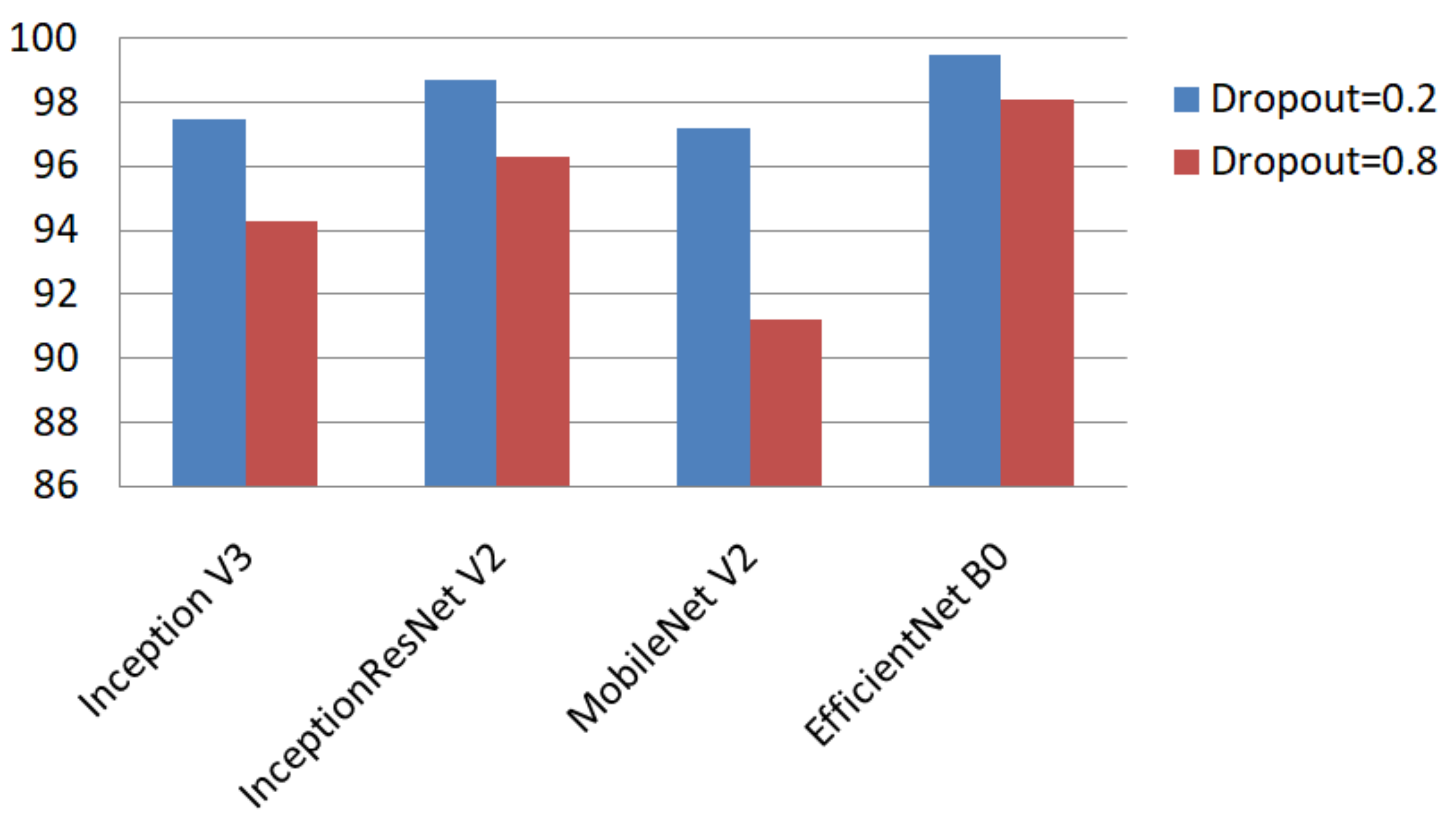
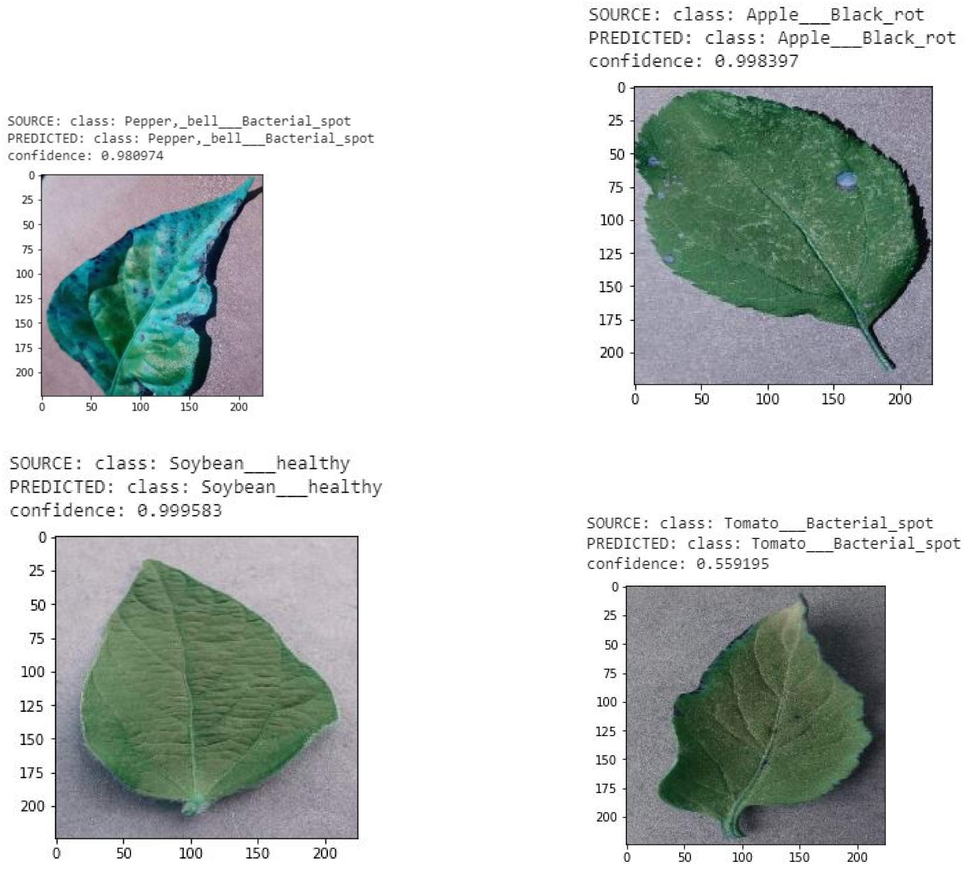
The accuracy of the model with respect to the number of predictions in the MobileNetV2 architecture decreased to 91% if we used a dropout value of 0.8. Figure 8 shows performance accuracy with respect to the different dropout values used in the network. Figure 9 shows correctly classified results from the test image dataset with their predicted and source class. The predicted class was returned with the confidence of that class.

5. Discussion

The early detection and identification of plant diseases using deep-learning techniques has recently made tremendous progress. Identification using traditional approaches heavily depends on some factors such as image enhancement, the segmentation of disease regions, and feature extraction.

Our approach is based on the identification of diseases using a deep-learning-based transfer-learning approach. Instead of using standard convolution, we used depthwise separable convolution in the inception block, which reduced the number of parameters by a large margin. To use both the inception and the residual network connection layer, we used the InceptionResNetV2 model. The model both has higher accuracy and requires less training time than the original architecture does, as the used parameters are much fewer. To check the performance towards a smartphone-implemented lightweight model to assist in plant-disease diagnosis, we implemented the MobileNetV2 model. We also implemented EfficientNetB0, which considers depth, width, and resolution during convolution.

Although the convolutional-neural-network-based deep-learning architecture achieved high success rates in the detection of plant diseases, it has some limitations, and there is a scope for future works. A little noise in the sample images led to misclassification by the deep-learning model [55,56]. Future work includes evaluating performance on noisy images and improving it. The dataset that we used to evaluate performance included 38 different diseases and healthy leaves. However, there is a need for the expansion of the dataset with wider land areas and more varieties of disease images. The dataset can also be improved with aerial photos, which are captured by drones. Another important issue is that the testing images are all from the same image dataset. Testing the network with real-time field images is an important challenging issue. The images that were used to test performance were all captured in laboratory conditions. The images that we used for testing our model are part of the same dataset, the training dataset. There is a need for the development of an efficient machine-learning system that could identify diseases in real-time scenarios and from collected data from different datasets. Some researchers are working on this field; they tested their model with real-time images, and performance worsened by a huge margin—around 25–30%. Mohanty et al. [24] conducted an experiment where they tested their model with different images from those in the training dataset and achieved an accuracy rate of 31.5%. Ferentinos et al. [25] measured performance with training images in laboratory conditions and tested the images in real-time conditions, and achieved an accuracy rate of 33%. To improve this, we need wide variety in databases, for example, with images taken in different lighting conditions, from different geographical areas, and with cultivating conditions. In addition, we aim to carry this research forward by implementing it with a new deep-learning model, such as ACNet [57], and a transformer-based architecture, such as ViT [58] and the MLP Mixer [59] method, in plant disease identification, and evaluate its performance.

6. Conclusions

There are many developed methods in the detection and classification of plant diseases using diseased leaves of plants. However, there is still no efficient and effective commercial solution that can be used to identify the diseases. In our work, we used four different DL models (InceptionV3, InceptionResnetV2, MobileNetV2, EfficientNetB0) for the detection of plant diseases using healthy- and diseased-leaf images of plants. To train and test the model, we used the standard PlantVillage dataset with 53,407 images, which were all captured in laboratory conditions. This dataset consists of 38 different classes of different healthy- and diseased-leaf images of 14 different species. After splitting the dataset into 80–20 (80% of whole data for training, 20% whole images for testing), we achieved the best accuracy rate of 99.56% in EfficientNetB0 model. On average, less time was required to train the images in the MobileNetV2 and EfficientNetB0 architectures, and it took 565 and 545 s/epoch, respectively, on colored images. In comparison with other deep-learning approaches, the implemented deep-learning model has better predictive ability in terms of both accuracy and loss. The required time to train the model was much less than that of other machine-learning approaches. Moreover, the MobileNetV2 architecture is an optimized deep convolutional neural network that limits the parameter number and operations as much as possible, and can easily run on mobile devices.

References

- Sethy, P.K.; Barpanda, N.K.; Rath, A.K.; Behera, S.K. Deep feature based rice leaf disease identification using support vector machine. Comput. Electron. Agric. 2020, 175, 105527. [Google Scholar]
- Chen, J.; Chen, J.; Zhang, D.; Sun, Y.; Nanehkaran, Y.A. Using deep transfer learning for image-based plant disease identification. Comput. Electron. Agric. 2020, 173, 105393. [Google Scholar]
- Bai, X.; Cao, Z.; Zhao, L.; Zhang, J.; Lv, C.; Li, C.; Xie, J. Rice heading stage automatic observation by multi-classifier cascade based rice spike detection method. Agric. For. Meteorol. 2018, 259, 260–270. [Google Scholar] [CrossRef]
- Ramcharan, A.; Baranowski, K.; McCloskey, P.; Ahmed, B.; Legg, J.; Hughes, D.P. Deep Learning for Image-Based Cassava Disease Detection. Front. Plant Sci. 2017, 8, 1852. [Google Scholar] [CrossRef] [Green Version]
- Camargo, A.; Smith, J. An image-processing based algorithm to automatically identify plant disease visual symptoms. Biosyst. Eng. 2009, 102, 9–21. [Google Scholar]
- Singh, J.; Kaur, H. Plant disease detection based on region-based segmentation and KNN classifier. In Proceedings of the International Conference on ISMAC in Computational Vision and Bio-Engineering 2018, Palladam, India, 16–17 May 2018; pp. 1667–1675. [Google Scholar]
- Camargo, A.; Smith, J. Image pattern classification for the identification of disease causing agents in plants. Comput. Electron. Agric. 2009, 66, 121–125. [Google Scholar]
- Chaudhary, A.; Kolhe, S.; Kamal, R. An improved random forest classifier for multi-class classification. Inf. Process. Agric. 2016, 3, 215–222. [Google Scholar]
- Phadikar, S.; Sil, J.; Das, A.K. Rice diseases classification using feature selection and rule generation techniques. Comput. Electron. Agric. 2013, 90, 76–85. [Google Scholar] [CrossRef]
- Munisami, T.; Ramsurn, M.; Kishnah, S.; Pudaruth, S. Plant leaf recognition using shape features and colour histogram with K-nearest neighbour classifiers. Procedia Comput. Sci. 2015, 58, 740–747. [Google Scholar]
- Ebrahimi, M.; Khoshtaghaza, M.; Minaei, S.; Jamshidi, B. Vision-based pest detection based on SVM classification method. Comput. Electron. Agric. 2017, 137, 52–58. [Google Scholar] [CrossRef]
- Garcia-Ruiz, F.; Sankaran, S.; Maja, J.M.; Lee, W.S.; Rasmussen, J.; Ehsani, R. Comparison of two aerial imaging platforms for identification of Huanglongbing-infected citrus trees. Comput. Electron. Agric. 2013, 91, 106–115. [Google Scholar] [CrossRef]
- Yao, Q.; Guan, Z.; Zhou, Y.; Tang, J.; Hu, Y.; Yang, B. Application of support vector machine for detecting rice diseases using shape and color texture features. In Proceedings of the 2009 International Conference on Engineering Computation, Hong Kong, China, 2–3 May 2009; pp. 79–83. [Google Scholar]
- Islam, M.; Dinh, A.; Wahid, K.; Bhowmik, P. Detection of potato diseases using image segmentation and multiclass support vector machine. In Proceedings of the 2017 IEEE 30th Canadian Conference on Electrical and Computer Engineering (CCECE), Windsor, ON, Canada, 30 April–3 May 2017; pp. 1–4. [Google Scholar]
- Tan, J.W.; Chang, S.W.; Kareem, S.B.A.; Yap, H.J.; Yong, K.T. Deep Learning for Plant Species Classification using Leaf Vein Morphometric. IEEE/ACM Trans. Comput. Biol. Bioinform. 2018, 17, 82–90. [Google Scholar] [CrossRef] [PubMed]
- McCallum, A.; Nigam, K. A comparison of event models for naive bayes text classification. In Proceedings of the AAAI-98 Workshop on Learning for Text Categorization, Madison, WI, USA, 26–27 July 1998; Volume 752, pp. 41–48. [Google Scholar]
- ÖZTÜRK, A.E.; Ceylan, M. Fusion and ANN based classification of liver focal lesions using phases in magnetic resonance imaging. In Proceedings of the 2015 IEEE 12th International Symposium on Biomedical Imaging (ISBI), Brooklyn, NY, USA, 16–19 April 2015; pp. 415–419. [Google Scholar]
- Pujari, D.; Yakkundimath, R.; Byadgi, A.S. SVM and ANN based classification of plant diseases using feature reduction technique. IJIMAI 2016, 3, 6–14. [Google Scholar] [CrossRef] [Green Version]
- Lee, S.H.; Chan, C.S.; Mayo, S.J.; Remagnino, P. How deep learning extracts and learns leaf features for plant classification. Pattern Recognit. 2017, 71, 1–13. [Google Scholar] [CrossRef] [Green Version]
- Shah, M.P.; Singha, S.; Awate, S.P. Leaf classification using marginalized shape context and shape+ texture dual-path deep convolutional neural network. In Proceedings of the 2017 IEEE International Conference on Image Processing (ICIP), Beijing, China, 17–20 September 2017; pp. 860–864. [Google Scholar]
- Li, Y.; Yang, J. Few-shot cotton pest recognition and terminal realization. Comput. Electron. Agric. 2020, 169, 105240. [Google Scholar] [CrossRef]
- Lee, S.H.; Goëau, H.; Bonnet, P.; Joly, A. New perspectives on plant disease characterization based on deep learning. Comput. Electron. Agric. 2020, 170, 105220. [Google Scholar] [CrossRef]
- Fuentes, A.; Yoon, S.; Kim, S.C.; Park, D.S. A robust deep-learning-based detector for real-time tomato plant diseases and pests recognition. Sensors 2017, 17, 2022. [Google Scholar] [CrossRef] [Green Version]
- Mohanty, S.P.; Hughes, D.P.; Salathé, M. Using deep learning for image-based plant disease detection. Front. Plant Sci. 2016, 7, 1419. [Google Scholar] [CrossRef] [Green Version]
- Ferentinos, K.P. Deep learning models for plant disease detection and diagnosis. Comput. Electron. Agric. 2018, 145, 311–318. [Google Scholar] [CrossRef]
- Sladojevic, S.; Arsenovic, M.; Anderla, A.; Culibrk, D.; Stefanovic, D. Deep neural networks based recognition of plant diseases by leaf image classification. Comput. Intell. Neurosci. 2016, 2016, 1–10. [Google Scholar] [CrossRef] [PubMed] [Green Version]
- Too, E.C.; Yujian, L.; Njuki, S.; Yingchun, L. A comparative study of fine-tuning deep learning models for plant disease identification. Comput. Electron. Agric. 2019, 161, 272–279. [Google Scholar] [CrossRef]
- Hussain, M.; Bird, J.J.; Faria, D.R. A study on cnn transfer learning for image classification. In UK Workshop on Computational Intelligence; Springer: Berlin/Heidelberg, Germany, 2018; pp. 191–202. [Google Scholar]
- Tan, M.; Le, Q. Efficientnet: Rethinking model scaling for convolutional neural networks. In Proceedings of the 2019 International Conference on Machine Learning, Long Beach, CA, USA, 9–15 June 2019; pp. 6105–6114. [Google Scholar]
- Mokhtar, U.; Ali, M.A.; Hassanien, A.E.; Hefny, H. Identifying two of tomatoes leaf viruses using support vector machine. In Information Systems Design and Intelligent Applications; Springer: Berlin/Heidelberg, Germany, 2015; pp. 771–782. [Google Scholar]
- Kaur, S.; Pandey, S.; Goel, S. Semi-automatic Leaf Disease Detection and Classification System for Soybean Culture. IET Image Process. 2018, 12, 1038–1048. [Google Scholar] [CrossRef]
- Babu, M.P.; Rao, B.S. Leaves Recognition Using Back Propagation Neural Network-Advice for Pest and Disease Control on Crops. Available online: https://citeseerx.ist.psu.edu/viewdoc/download?doi=10.1.1.110.3632&rep=rep1&type=pdf (accessed on 1 May 2021).
- Chouhan, S.S.; Kaul, A.; Singh, U.P.; Jain, S. Bacterial foraging optimization based radial basis function neural network (BRBFNN) for identification and classification of plant leaf diseases: An automatic approach towards plant pathology. IEEE Access 2018, 6, 8852–8863. [Google Scholar] [CrossRef]
- Kamilaris, A.; Prenafeta-Boldú, F.X. Deep learning in agriculture: A survey. Comput. Electron. Agric. 2018, 147, 70–90. [Google Scholar] [CrossRef] [Green Version]
- Geetharamani, G.; Pandian, A. Identification of plant leaf diseases using a nine-layer deep convolutional neural network. Comput. Electr. Eng. 2019, 76, 323–338. [Google Scholar]
- Jadhav, S.B.; Udupi, V.R.; Patil, S.B. Identification of plant diseases using convolutional neural networks. Int. J. Inf. Technol. 2020, 1–10. [Google Scholar] [CrossRef]
- Rangarajan Aravind, K.; Raja, P. Automated disease classification in (Selected) agricultural crops using transfer learning. Autom. Časopis Autom. Mjer. Elektron. Računarstvo Komun. 2020, 61, 260–272. [Google Scholar] [CrossRef]
- Rangarajan, A.K.; Purushothaman, R. Disease classification in eggplant using pre-trained vgg16 and msvm. Sci. Rep. 2020, 10, 1–11. [Google Scholar]
- Arora, J.; Agrawal, U. Classification of Maize leaf diseases from healthy leaves using Deep Forest. J. Artif. Intell. Syst. 2020, 2, 14–26. [Google Scholar] [CrossRef] [Green Version]
- Ghazi, M.M.; Yanikoglu, B.; Aptoula, E. Plant identification using deep neural networks via optimization of transfer learning parameters. Neurocomputing 2017, 235, 228–235. [Google Scholar] [CrossRef]
- Li, Y.; Nie, J.; Chao, X. Do we really need deep CNN for plant diseases identification? Comput. Electron. Agric. 2020, 178, 105803. [Google Scholar] [CrossRef]
- Zeng, W.; Li, M. Crop leaf disease recognition based on Self-Attention convolutional neural network. Comput. Electron. Agric. 2020, 172, 105341. [Google Scholar] [CrossRef]
- Oyewola, D.O.; Dada, E.G.; Misra, S.; Damaševičius, R. Detecting cassava mosaic disease using a deep residual convolutional neural network with distinct block processing. PeerJ Comput. Sci. 2021, 7, e352. [Google Scholar] [CrossRef] [PubMed]
- Ramcharan, A.; McCloskey, P.; Baranowski, K.; Mbilinyi, N.; Mrisho, L.; Ndalahwa, M.; Legg, J.; Hughes, D.P. A mobile-based deep learning model for cassava disease diagnosis. Front. Plant Sci. 2019, 10, 272. [Google Scholar] [CrossRef] [PubMed] [Green Version]
- Adedoja, A.; Owolawi, P.A.; Mapayi, T. Deep learning based on NASNet for plant disease recognition using leave images. In Proceedings of the 2019 International Conference on Advances in Big Data, Computing and Data Communication Systems (icABCD), Winterton, South Africa, 5–6 August 2019; pp. 1–5. [Google Scholar]
- Zhao, Y.; Chen, Z.; Gao, X.; Song, W.; Xiong, Q.; Hu, J.; Zhang, Z. Plant Disease Detection using Generated Leaves Based on DoubleGAN. IEEE ACM Trans. Comput. Biol. Bioinform. 2021. [Google Scholar] [CrossRef] [PubMed]
- Simonyan, K.; Zisserman, A. Very deep convolutional networks for large-scale image recognition. arXiv 2014, arXiv:1409.1556. [Google Scholar]
- Russakovsky, O.; Deng, J.; Su, H.; Krause, J.; Satheesh, S.; Ma, S.; Huang, Z.; Karpathy, A.; Khosla, A.; Bernstein, M.; et al. ImageNet Large Scale Visual Recognition Challenge. Int. J. Comput. Vis. (IJCV) 2015, 115, 211–252. [Google Scholar] [CrossRef] [Green Version]
- Szegedy, C.; Ioffe, S.; Vanhoucke, V.; Alemi, A. Inception-v4, inception-resnet and the impact of residual connections on learning. In Proceedings of the AAAI Conference on Artificial Intelligence 2017, San Francisco, CA, USA, 4–9 February 2017; Volume 31. [Google Scholar]
- He, K.; Zhang, X.; Ren, S.; Sun, J. Deep residual learning for image recognition. In Proceedings of the IEEE Conference on Computer Vision and Pattern Recognition, Las Vegas, NV, USA, 27–30 June 2016; pp. 770–778. [Google Scholar]
- Howard, A.G.; Zhu, M.; Chen, B.; Kalenichenko, D.; Wang, W.; Weyand, T.; Andreetto, M.; Adam, H. Mobilenets: Efficient convolutional neural networks for mobile vision applications. arXiv 2017, arXiv:1704.04861. [Google Scholar]
- Sandler, M.; Howard, A.; Zhu, M.; Zhmoginov, A.; Chen, L.C. Mobilenetv2: Inverted residuals and linear bottlenecks. In Proceedings of the IEEE Conference on Computer Vision and Pattern Recognition 2018, Salt Lake City, UT, USA, 18–23 June 2018; pp. 4510–4520. [Google Scholar]
- Plant Village Dataset. Available online: https://github.com/spMohanty/PlantVillage-Dataset (accessed on 16 February 2019).
- Toda, Y.; Okura, F. How convolutional neural networks diagnose plant disease. Plant Phenomics 2019, 2019, 1–14. [Google Scholar] [CrossRef]
- Kwon, H.; Yoon, H.; Park, K.W. Acoustic-decoy: Detection of adversarial examples through audio modification on speech recognition system. Neurocomputing 2020, 417, 357–370. [Google Scholar] [CrossRef]
- Kwon, H.; Yoon, H.; Choi, D. Restricted evasion attack: Generation of restricted-area adversarial example. IEEE Access 2019, 7, 60908–60919. [Google Scholar] [CrossRef]
- Hu, X.; Yang, K.; Fei, L.; Wang, K. Acnet: Attention based network to exploit complementary features for rgbd semantic segmentation. In Proceedings of the 2019 IEEE International Conference on Image Processing (ICIP), Taipei, Taiwan, 22–25 September 2019; pp. 1440–1444. [Google Scholar]
- Dosovitskiy, A.; Beyer, L.; Kolesnikov, A.; Weissenborn, D.; Zhai, X.; Unterthiner, T.; Dehghani, M.; Minderer, M.; Heigold, G.; Gelly, S.; et al. An image is worth 16x16 words: Transformers for image recognition at scale. arXiv 2020, arXiv:2010.11929. [Google Scholar]
- Tolstikhin, I.; Houlsby, N.; Kolesnikov, A.; Beyer, L.; Zhai, X.; Unterthiner, T.; Yung, J.; Keysers, D.; Uszkoreit, J.; Lucic, M.; et al. Mlp-mixer: An all-mlp architecture for vision. arXiv 2021, arXiv:2105.01601. [Google Scholar]
Figure 1.
Basic architectures of implemented DL models.
Figure 2.
Basic block diagram of InceptionResNetV2 model.
Figure 3.
(a) Modified structures of InceptionResnet-A. (b) Structures of InceptionResnet-B of InceptionResNetV2 model.
Figure 4.
Structures of InceptionResNet-C in InceptionResNetV2.
Figure 5.
Basic block diagram of EfficientNet model.
Figure 6.
Sample images of color, grayscale and segmented version of PlantVillage image dataset.
Figure 7.
(a) Performance accuracy of implemented model. (b) Performance loss of implemented model. (c) F1 score of InceptionV3. (d) Accuracy of InceptionResNetV2 grouped by training.
Figure 8.
Performance accuracy with different dropout values.
Figure 9.
Example of correct classification from test image set.