Optimal Placement and Sizing of D-STATCOM in Radial and Meshed Distribution Networks Using a Discrete-Continuous Version of the Genetic Algorithm

Abstract

In this paper, we propose a new discrete-continuous codification of the Chu–Beasley genetic algorithm to address the optimal placement and sizing problem of the distribution static compensators (D-STATCOM) in electrical distribution grids. The discrete part of the codification determines the nodes where D-STATCOM will be installed. The continuous part of the codification regulates their sizes. The objective function considered in this study is the minimization of the annual operative costs regarding energy losses and installation investments in D-STATCOM. This objective function is subject to the classical power balance constraints and devices’ capabilities. The proposed discrete-continuous version of the genetic algorithm solves the mixed-integer non-linear programming model that the classical power balance generates. Numerical validations in the 33 test feeder with radial and meshed configurations show that the proposed approach effectively minimizes the annual operating costs of the grid. In addition, the GAMS software compares the results of the proposed optimization method, which allows demonstrating its efficiency and robustness.

1. Introduction

In electrical power systems, some problems correspond to the high values of energy losses [1]. In addition, these losses are significantly higher in percentage terms in distribution systems, when compared to transmission networks due to the voltage levels used and the radial topology with which they are built [2]. Around the world, electricity distribution networks are the channels that supply electricity to millions of end-users. Furthermore, in the Colombian context, the distribution of electrical energy is carried out at medium and low voltage levels, i.e., with operational voltages typically between 10 kV and 15 kV [3]. The construction of distribution networks usually uses radial topology to minimize investment costs in conductors and protection elements. However, the main problem with these topologies corresponds to the high percentages of energy losses that can occur [2,4].

Losses of power in the supply of energy to consumers represent considerable economic losses for the companies that provide the service. A high percentage of losses in the distribution network produces a reduction in income. It is due to the unbilled energy, which manifests itself as an increase in the rates for the end-users of the service. In the Colombian context, the electrical system has energy losses of around 1.5% to 2.0% of the total energy generated. In medium voltage networks, energy losses can vary from 5% to 18% [2]. Loss levels lower than 10% correspond to networks in which, in compliance with the requirements of regulatory entities, maintenance has been carried out along with replacement of equipment. Levels above 10% are related to the inadequate management of distribution assets [2]. Additionally, since 2007, the Energy and Gas Regulation Commission (CREG), through CREG resolution number 121, limits the maximum charge for losses (13%) transfer to users of electricity service in Colombia [5]. If the losses show an increase concerning this limit, the network operator must assume the differential [5].

To address the technical and economic problems caused by energy losses in distribution networks. The specialized literature proposes different methodologies to reduce technical losses in distribution networks [1]. These methodologies are the location of distributed generation [6], reconfiguration of primary feeders [7], and a connection of shunt capacitors [8,9]. In the same way, distributed generation is the best option to reduce power losses. However, their initial installation costs can be very high compared to strategies such as reconfiguration and shunt capacitor connection [2]. The main problem with capacitor banks is that they inject reactive power in fixed steps of reactive power. They do not consider that the daily demand for active and reactive power along the electrical distribution networks is variable and continuous. In recent years, compensators based on power electronics have gained importance [10] to solve the compensation challenges based on shunt capacitors. Distribution networks utilize these mechanisms due to their versatility and ability to vary reactive power injections depending on the demand. These devices are known as static power compensators (D-STATCOM) [10]. The D-STATCOM implementation presents some relevant advantages, such as (i) high reliability, (ii) low operating costs, and (iii) long useful life (typically 5 to 15 years) [2]. This article proposes the installation and optimal sizing of D-STATCOM in distribution systems to reduce annual operating costs associated with energy losses. The variables of interest in this work will be the size and optimal location of these devices through the distribution network [11].

In the specialized literature, the problem of optimal location and dimensioning of D-STATCOM has been explored mainly through metaheuristic methods; below, some of them are presented. The authors in [12] represent the application of an imperialist competition algorithm to find the optimal location and dimensioning of D-STATCOM in distribution networks. The objectives of the optimization problem are the voltage profile index, the load balance index, and the annual cost savings index. The previous mains are combined to obtain a general objective function using a Max-geometric mean operator. The authors validate the proposed methodology in test systems of 33 and 69 nodes. In addition, they take into account the variability of the system load from a fuzzy technique. The performance of the proposed methodology is slightly better than the bacterial foraging optimization algorithm [13], the secure hash algorithm [14], and the immune algorithm [15], respectively.

The authors in [16] propose an optimization method based on a multi-target particle swarm algorithm; this allows finding the optimal location and dimensioning of D-STATCOM in distribution systems. This method takes into account the possibility of reconfiguring the network for different demand scenarios. The objective function of the problem considers the minimization of active power losses, the voltage stability index, and the load factor of the distribution networks. The algorithm works only under maximum load conditions. Although the results obtained are adequate, working with peak demand can lead to oversizing of the D-STATCOM.

In [17], an ant colony optimization algorithm is worked that integrates a multi-objective fuzzy technique. This work proposes the simultaneous realization of a reconfiguration and the assignment (location and dimensioning) of photovoltaic sources and D-STATCOM in distribution systems. The objective was to minimize network losses and improve voltage profiles. The IEEE 33-node system implements the algorithm. The authors of [18] propose a heuristic method based on power and voltage loss indicators to optimally locate and size D-STATCOM in radial networks to reduce energy losses. However, the authors only consider a peak demand scenario. On the IEEE 33-node system, computational validations are performed.

The authors of [19] present an optimization strategy based on the bio-inspired search algorithm in the cuckoo bird for the location and sizing of D-STATCOM. In this work, from the loss sensitivity factor, the optimal location of the D-STATCOM is determined; while through CSA, the capacity of the D-STATCOM is calculated. By a method of successive approximations, the power flow is calculated. The objective function of the problem is the reduction of the total power losses of the system. To demonstrate the efficiency of the algorithm, IEEE 33- and IEEE 69-node systems are used.

Table 1. Summary of methodologies used in the literature for the location and dimensioning of D-STATCOM.

Solution Methodology	Objective Function	Ref.	Year
Genetic algorithm	Power losses minimization	[20]	2011
Ant colony optimization	Power losses minimization and voltage profile improvement	[17]	2015
Sensitivity indexes	Power losses minimization	[18]	2015
Harmony search algorithm	Power losses minimization	[14]	2015
Heuristic search algorithm	Power losses minimization	[21]	2016
Imperialist competitive algorithm	Minimization of energy costs and voltage profile improvement	[12]	2017
Modified crow search algorithm	Voltage profile improvement, reduce line losses, maximize economic benefit, and decrease the pollution level	[22]	2018
Particle swarm optimization	Power losses reduction and voltage profile improvement	[16]	2019
Ant lion optimization algorithm	The system loss minimization and voltage profile improvement	[23]	2019
Hybrid analytical–coyote	Active power losses minimization and voltage profile improvement	[24]	2019
Modified sine cosine algorithm	Power losses minimization and voltage profile improvement	[25]	2020
Discrete-continuous vortex search algorithm	Investment and operating costs reduction	[2]	2021
Genetic algorithm and conic programming	Investment and operating costs reduction	[11]	2021
Solution of the exact MINLP model in the GAMS software	Investment and operating costs reduction	[26]	2021

represents a summary of the methodologies most used in the specialized literature for the dimensioning and location of D-STATCOM in distribution networks.

From the literature review presented in Table 1, we can note that: (i) most of the objective functions used to study the optimal placement and size D-STATCOM problem in distribution networks focus on minimizing the power losses (energy losses) and voltage profile improvement. A few of them consider investment and operating costs as will be analyzed in this proposal. (ii) In 2021, three recent approaches have introduced the investment and operative costs of the D-STATCOM considering daily active and reactive power curves into the analysis. (iii) Most of the optimization methodologies are based on the usage of metaheuristic algorithms to solve the problem and increase the possibility of escaping from local optimums. For these reasons, after reviewing the specialized literature, this article proposes the location and optimal dimensioning of D-STATCOM in distribution systems through a Chu and Beasley genetic algorithm (CBGA) [27], with coding that integrates discrete and continuous variables.

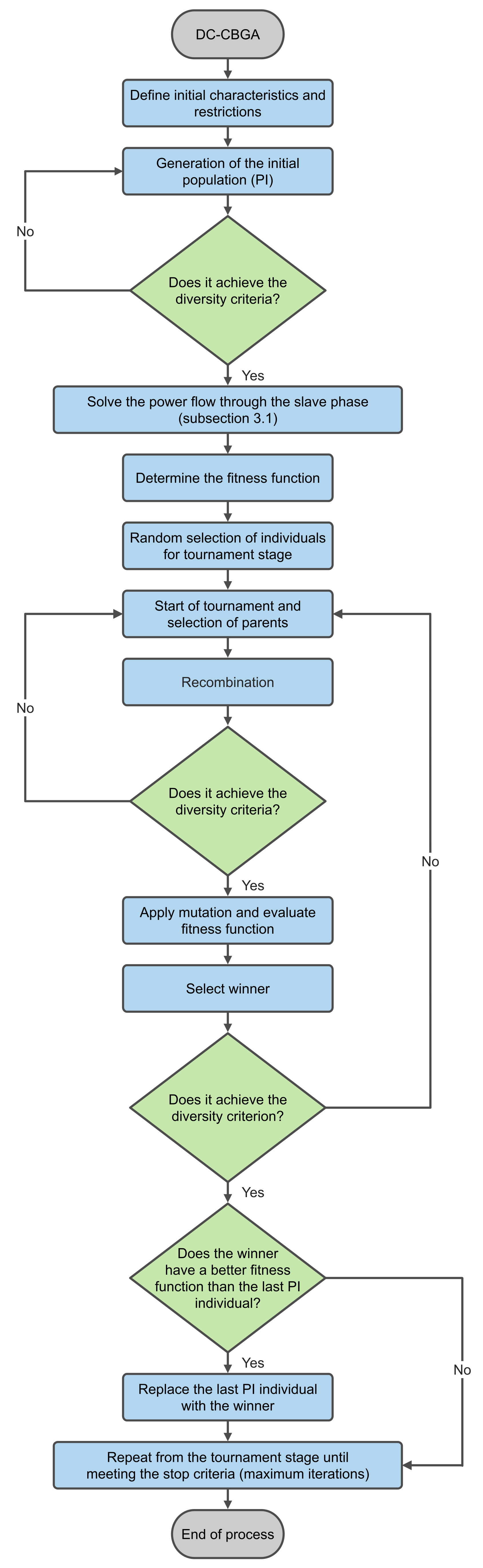
The discrete-continuous version of the CBGA proposed in this work will be called DC-CBGA. The specialized literature does not report any studies with these characteristics, implementing a unified codification with integer and continuous variables for the CBGA (the discrete part of the codification determines the nodes considering the location of the D-STATCOM, and the continuous part is in charge of their optimal dimensioning). This study proposed a master–slave methodology. The phase directed by the DC-CBGA and responsible for the dimensioning and location of the D-STATCOMs is the master phase. The slave phase is in charge of running the power flow whenever the master phase requires it. It is relevant to highlight that the proposed methodology is functional for radial and meshed topologies.

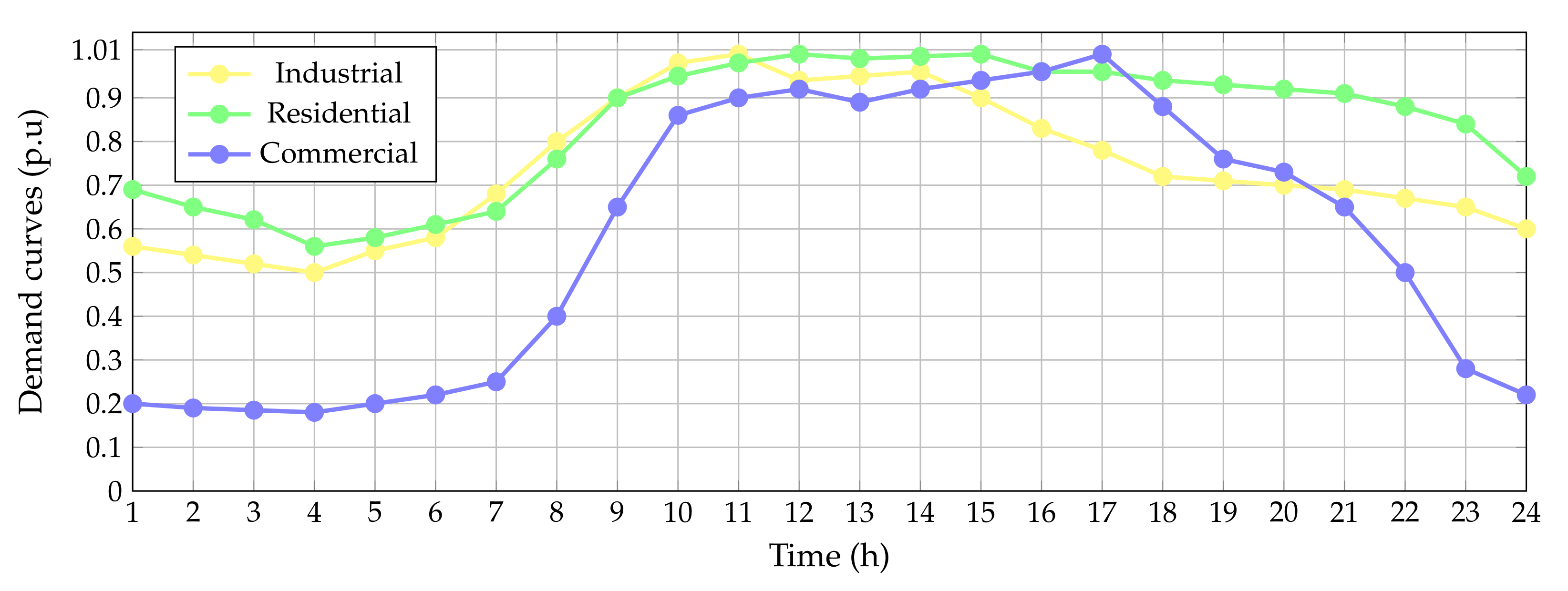
The slave phase uses the method of successive approximations that is compatible with both types of topology. In addition, it discriminates against the demand according to the application. According to the demand curve of the system, it categorizes three zones, residential, commercial, and industrial. Through a mixed-integer non-linear programming model (MINLP), the above mentioned is represented. The GAMS software compares the results obtained by the proposed methodology. It is relevant to highlight that using a unified codification with integer and continuous variables reduces the total processing time required to solve the problem compared with combined algorithms that divide the exploration of the solution space among discrete and continuous variables. In the same way, it considers the contribution of this research to the optimization with genetic algorithms that involves different types of variables.

The current literature presents three similar works regarding the optimal location and sizing of D-STATCOM in distribution networks. Authors in [2] present a master–slave optimization approach based on the discrete-continuous version of vortex search algorithm to locate and size D-STATCOM in distribution networks with a unified codification. Even if the codification is similar to the DC-CBGA, the main difference of our approach concerning this work corresponds to the possibility of analyzing radial and meshed distribution networks without any special modification to the power flow method in the slave optimization stage. In addition, we consider the effect of residential, industrial, and commercial loads distributed in different areas of the test feeder.

The authors of [11] have proposed a hybrid optimization methodology based on the combination of the CBGA and a second-order cone programming (SOCP) optimization. The CBGA is in charge of determining the nodes regarding the D-STACOM location, and the SOCP model solves the optimal multi-period power flow problem to establish the optimal D-STATCOM sizes; even though this methodology is efficient to solve the problem, it has three main difficulties: (i) the SOCP only works with pure-radial distribution networks; (ii) the SOCP only works with the minimization of the energy losses in the networks; and (iii) the processing times of the methodology can increase significantly as a function of the number of nodes in the distribution system. These difficulties imply that the costs of the final solution cannot be the global optimum due to the problem being solved in a decoupled way. The main advantage of the current proposal, based on the DC-CBGA, is that the methodology can deal with radial and meshed distribution networks with low computational effort. At the same time, the results initially reported in [11] are improved, which demonstrates that the Genetic-Convex approach stays stuck in a local optimum.

Finally, the authors of [26] have presented a generalized optimization model to locate and size STATCOM in power and distribution systems with radial or meshed topologies. To solve the exact MINLP optimization problem, the GAMS software and the BONMIN solver are used; however, the main issue of this methodology is the high probability of being stuck in a locally optimal solution due to 145, the non-linear non-convexity of the solution space. The main advantage of the proposed DC-CBGA is that the optimal solutions reaching the radial and meshed distribution configurations have better quality when compared to the GAMS software, i.e., the DC-CBGA can escape to the local optimums to explore more promissory solution regions.

The rest of this document is presented with the following order: Section 2 describes the general mixed-integer non-linear programming model representing the D-STATCOM location and sizing problem; this model considers a variant formulation in time that minimizes annual operating costs. Section 3 presents the master–slave stages of the solution model. First the slave phase (i.e., power flow through the successive approximations method) and then the master phase based on the discrete-continuous version of the CBGA. 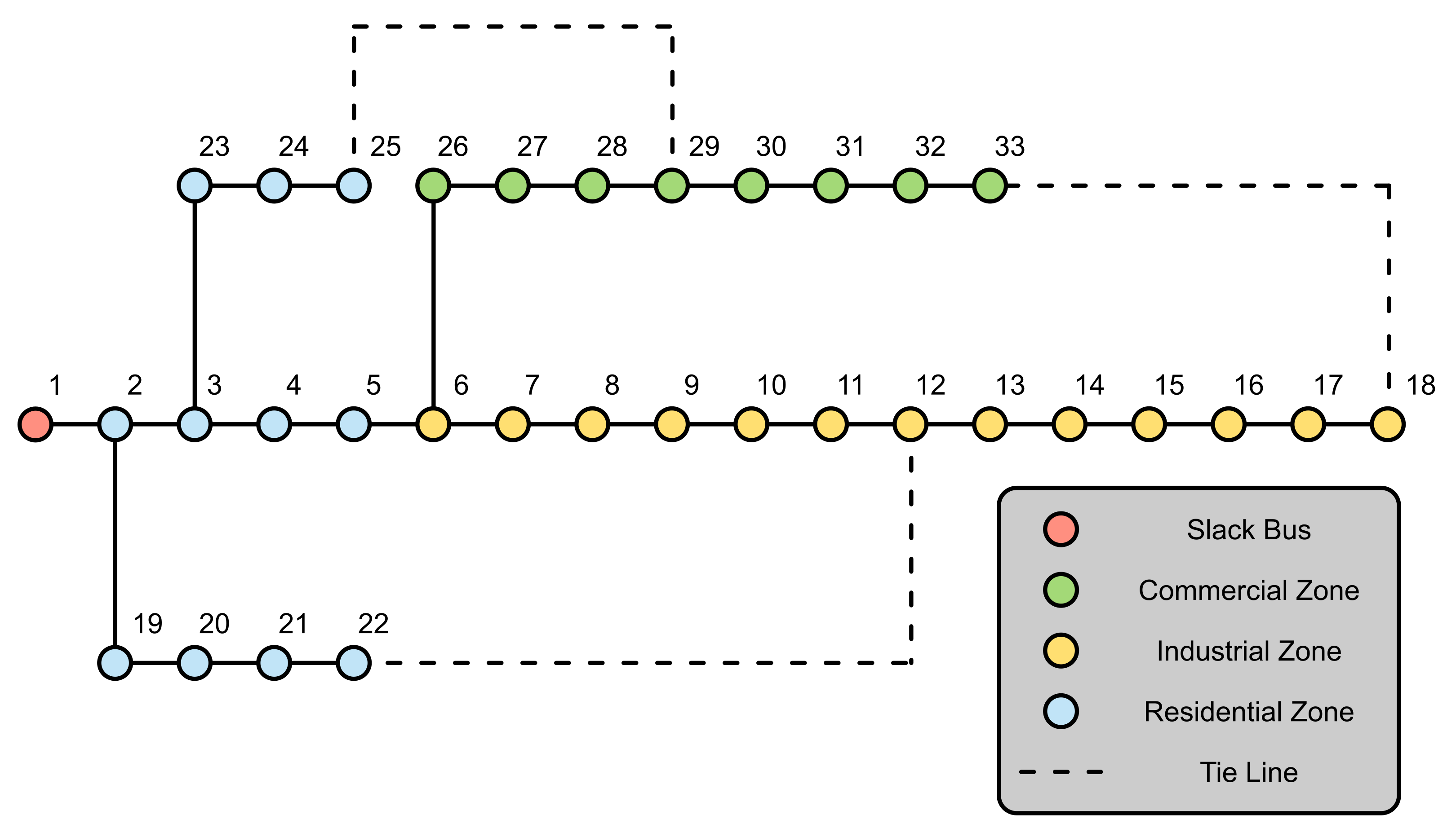Section 4 characterizes the networks used to evaluate the proposed methodology; it uses IEEE 33-node network with radial and meshed configurations. In Section 5, the results obtained are presented, contrasted, and analyzed. Finally, Section 6 contains conclusions.

2. Mathematical Modeling

This section presents the mathematical model of the optimal location and dimensioning problem of D-STATCOM in electrical power distribution systems with radial or meshed topologies. By containing this problem, a Mixed Integer Non-linear Programming (MINLP) model [26] can be represented as discrete variables (nodes where the D-STATCOM will be located) and continuous (size of the D-STATCOM). In addition, there will be an objective function, which is the sum of the costs for power losses for one year and the annualized investment costs related to the D-STATCOM. Below is presented the mathematical formulation of the problem under study.

2.1. Objective Function

The structure of each of the components that make up the objective function, i.e., the annual cost function of energy losses ($f_1$), and the annualized investment cost function of D-STATCOM ($f_2$), are defined through Equations (1) and (2).

$$f_1=C_{kWh}T\sum _{h\in \mathbb{H}}^{}\sum _{k\in \mathbb{N}}^{}\sum _{m\in \mathbb{N}}^{}{Y}_{km}{V}_{kh}{V}_{mh}cos\left({\delta }_{kh}-{\delta }_{mh}-{\theta }_{km}\right){\Delta }_h,$$

(1)

$$f_2=T\left(\frac{k_1}{k_2}\right)\sum _{k\in \mathbb{N}}^{}\left(\alpha {\left(Q_k^{DS}\right)}^2+\beta Q_k^{DS}+\gamma \right)Q_k^{DS}.$$

(2)

Equation (1) defines the annual cost functions of energy losses in all sections of the distribution network. $C_{kWh}$ is the average cost per $kWh$, T is a constant associated with the study period (365 days), $Y_{km}$ is the magnitude of the component associated nodal admittance matrix that relates the nodes k and m with an angle ${\theta }_{km}$, $V_{kh}$ and $V_{mh}$ are the voltages related to nodes k and m in period h with angles ${\delta }_{kh}$ and ${\delta }_{mh}$, respectively, ${\Delta }_h$ corresponds to the time associated with the power flow (1 h) evaluation. Finally, $\mathbb{H}$ and $\mathbb{N}$ are the sets that contain all the periods and all the nodes of the network, respectively.

Equation (2) is the annualized investment cost function of D-STATCOM, where $k_1$ and $k_2$ are positive constants. The first refers to the annualized investment costs, and the second refers to the useful life of the D-STATCOM. The parameters $\alpha$, $\beta$, and $\gamma$ are positive constants and correspond to the variable installation costs of D-STATCOM with nominal reactive power generation capacity, i.e., $Q_k^{DS}$. To obtain the general objective function of the problem (Equation (3)), we proceed to the algebraic sum of Equations (1) and (2).

$$min{A}_{\mathrm{cost}}=f_1+f_2$$

(3)

$A_{\mathrm{cost}}$ represents the annual operating cost of the network and the investment in D-STATCOM.

2.2. Definition of Restrictions

The constraints of the problem of location and dimensioning of D-STATCOM in distribution networks correspond to the maximum number of D-STATCOM, voltage regulation, active and reactive power balance, and power limit the D-STATCOM can provide. Equations (4)–(8) define the constraints for the problem under study.

$$P_{kh}^g-P_{kh}^d=\sum _{k\in \mathbb{N}}^{}\sum _{m\in \mathbb{N}}^{}{Y}_{km}{V}_{kh}{V}_{mh}cos\left({\delta }_{kh}-{\delta }_{mh}-{\theta }_{kh}\right),\forall \left\{k\in \mathbb{N}\&h\in \mathbb{H}\right\},$$

(4)

$$Q_{kh}^g+Q_k^{DS}-Q_{kh}^d=\sum _{k\in \mathbb{N}}^{}\sum _{m\in \mathbb{N}}^{}{Y}_{km}{V}_{kh}{V}_{mh}sin\left({\delta }_{kh}-{\delta }_{mh}-{\mathrm{\Theta }}_{km}\right),\forall \left\{k\in \mathbb{N}\&h\in \mathbb{H}\right\},$$

(5)

$$V_{min}\le V_{kh}\le V_{max},\forall \left\{k\in \mathbb{N}\&h\in \mathbb{H}\right\},$$

(6)

$$Z_k{Q}_{min}^{DS}\le Q_k^{DS}\le Z_k{Q}_{max}^{DS},\forall \left\{k\in \mathbb{N}\right\},$$

(7)

$$\sum _{k\in \mathbb{N}}^{}{Z}_k\le N_A^{DS}.$$

(8)

Equations (4) and (5) represent the balance of active and reactive power, respectively, for each node and period. It is relevant to highlight that in Equation (5), the variable $Q_k^{DS}$ is introduced, which will have the effect of injecting reactive power from the D-STATCOM in the nodes where they are assigned. Variables $P_{kh}^g$ and $Q_{kh}^g$ are the active and reactive power injections of the generator connected to node k in period h. $P_{kh}^d$ and $Q_{kh}^d$ are the active and reactive power demands of the loads connected to node k in time h. It is necessary to mention that these consumptions vary according to the average daily demand curve. The inequality in Equation (6) defines the upper and lower limits of voltage for each node’s network in each period. This restriction is due to impositions made by regulatory authorities of the electricity sector [28]. The constants $V_{min}$ and $V_{max}$ indicate the permitted voltage limits for all nodes. In Equation (7), the nominal reactive power limit for each D-STATCOM is shown, the binary variable $Z_k$ indicates whether or not the D-STATCOM is located at node k. The constants $Q_{min}^{DS}$ and $Q_{max}^{DS}$ are the upper and lower limits associated with the injection of reactive power from the D-STATCOM. The inequality (8) limits the number of installed D-STATCOM in the distribution network, where $N_A^{DS}$ is the maximum installed number in the distributed network.

It is necessary to mention that the mathematical model (1)–(8) is, as mentioned in the beginning, an MINLP type. This type is due to several variable types, as follows: continuous variables related to the generation of active and reactive power, including the magnitudes and angles of the nodal voltages; and binary variables associated with the location of the D-STATCOM on the network. Additionally, it has a non-linear structure due to the trigonometric functions and voltage products that present the active and reactive power balance restrictions [2].

3. Solution Methodology

For the solution of the MINLP (Equations (1)–(8)) model associated with the location and optimal dimensioning of D-STATCOM in electrical distribution networks proposed in Section 2, it suggests a master–slave optimization methodology [2]. The master phase uses a modified CBGA of a discrete-continuous nature. The slave phase employs the method of successive approximations. The master phase defines the nodes where the D-STATCOM and their optimal dimensions are located. On the other hand, the slave phase is in charge of determining the daily energy losses through the multi-period power flow solution [2]. Below are presented each of these phases.

3.1. Slave Stage: Power Flow

The slave phase utilizes the successive approximations method. This method is in charge of determining the power flow for each period h [29,30]. The slave stage has a task illustrating the effects of the operational changes caused by the inclusion of D-STATCOM in the network assigned by the master stage. To solve the power balance restriction in Equations (4) and (5) is necessary to rewrite them in their complex form, as observed in Equations (9) and (10) [29].

$${\mathbf{S}}_{sh}^{*}=\mathrm{diag}\left({\mathbf{V}}_{\mathbf{sh}}^{*}\right)\left[{\mathbb{Y}}_{ss}{\mathbf{V}}_{\mathbf{sh}}+{\mathbb{Y}}_{sd}{\mathbf{V}}_{\mathbf{dh}}\right],\forall \left\{h\in \mathbb{H}\right\},$$

(9)

$${\mathbf{S}}_{qh}^{*}-{\mathbf{S}}_{dh}^{s,*}=\mathrm{diag}\left({\mathbf{V}}_{\mathbf{dh}}^{*}\right)\left[{\mathbb{Y}}_{ds}{\mathbf{V}}_{\mathbf{sh}}+{\mathbb{Y}}_{dd}{\mathbf{V}}_{\mathbf{dh}}\right],\forall \left\{h\in \mathbb{H}\right\}.$$

(10)

where ${\mathbf{S}}_{sh}^{*}$ is the complex vector that contains all the apparent power generation at the slack node for each period h, ${\mathbf{V}}_{sh}^{*}$ is the complex vector that holds all the voltages of the slack nodes for each time h, ${\mathbf{V}}_{dh}^{*}$ is a vector that contains all the voltages of the demand nodes, in their complex form, in each time h, ${\mathbb{Y}}_{ss}$, ${\mathbb{Y}}_{sd}$, ${\mathbb{Y}}_{ds}$, and ${\mathbb{Y}}_{dd}$ are sub-matrices obtained from the matrix of nodal admittances that relate the slack and demand nodes, respectively. ${\mathbf{S}}_{qh}^{*}$ and ${\mathbf{S}}_{dh}^{*}$ contain the reactive powers generated by the D-STATCOM and the apparent power demanded for each period h, respectively. Note that ${\mathbf{V}}_{sh}$ is a known variable since these correspond to the voltages of the slack nodes, while ${\mathbf{V}}_{dh}$ is an unknown variable that is necessary to determine in each period. To find the unknown variables ${\mathbf{V}}_{dh}$, Equation (11) is applied iteratively, which is the result of rearranging Equation (10) as recommended in [29] to solve the power flow problem through the successive approximation method. For this to be possible, the reactive power injections of the D-STATCOM must be known, which is provided by the master stage [2].

$${\mathbf{V}}_{dh}^{m+1}={\mathbb{Y}}_{dd}^{-1}\left[{\mathrm{diag}}^{-1}\left({\mathbf{V}}_{dh}^{m,*}\right)\left[{\mathbf{S}}_{qh}^{m,*}-{\mathbf{S}}_{dh}^{s,*}\right]-{\mathbb{Y}}_{ds}{\mathbf{V}}_{sh}\right],\forall \left\{h\in \mathbb{H}\right\}.$$

(11)

m corresponds to the iteration counter. When m equals zero, ${\mathbf{V}}_{dh}^0=1\angle 0^{\circ }$ defines the initial values as the initial voltage condition using the per-unit representation. As the counter advances, it updates the values with those obtained in the immediately previous iteration. The iterative process ends when the program reaches the stop criterion, defined through Equation (12).

$$max\left\{\left|\left|{\mathbf{V}}_{dh}^{m+1}\right|-\left|{\mathbf{V}}_{dh}^m\right|\right|\right\}\le ϵ.$$

(12)

In Equation (12), the criterion presented must be reached before the maximum number of iterations, where $ϵ$ is the assigned tolerance. Convergence is guaranteed since the successive approximation method corresponds to a contraction map, and therefore converges whenever the initial system is far from the stress collapse point [30].

3.2. Master Algorithm: Discrete-Continuous Genetic Algorithm

The master phase is the one in charge of making modifications to the network throughout the implementation of the D-STATCOM [29]. Restrictions that help the method find the optimal configuration have directed this process. This article proposes a discrete-continuous version of the CBGA. The hybrid DC CBGA configuration determines the nodes where the D-STATCOM are located (discrete part) and their sizes (continuous side).

The CBGA is part of the metaheuristic evolutionary computation methods based on Darwin’s theory of evolution, i.e., the natural selection process present in nature [31]. Mathematically, it is considered a combinatorial optimization technique. This technique has a high probability of finding global explanations for complex problems of great size and along multiple local optima [32]. In the case of electrical engineering, they have been used successfully in problems as electrical demand control [31], reactive power compensation in primary distribution circuits [29], reconfiguration of distribution systems [33], and the location of devices based on power electronics [34]. The implementation of this optimization strategy involves the following stages: selection, recombination, and mutation [33]. Below are some details about the proposed encoding and the phases that make up the CBGA.

First, the algorithm creates (I) individuals randomly in the limits established for the population; the creation of these individuals follows the model described in Equation (13).

$$\begin{gathered} X_I=\left[U_1^{DS},...,U_{N_A}^{DS}⋮Q_1^{DS},...,Q_{N_A}^{DS}\right], \\ {X}_{min}=\left[2,...,2⋮Q_{min}^{DS},...,Q_{min}^{DS}\right] \\ {X}_{max}=\left[N,...,N⋮Q_{max}^{DS},...,Q_{max}^{DS}\right] \\ {X}_i=X_{min}+\mathrm{rand}\left(1\right)·(X_{max}-X_{min}) \end{gathered}$$

(13)

.

Equation (13) represents how the algorithm creates each individual. Vector $X_I$ corresponds to the generic form of individual I. This arrangement divides into two parts of an equal number of positions. The first part is discrete; it contains the nodal area, where D-STATCOM ($U_{N_A}^{DS}$) is localized. The second is continuous in nature and stores the sizes of the D-STATCOM ($Q_{N_A}^{DS}$). $X_{min}$ and $X_{max}$ are the lower and upper bounds for the population. Its discrete part is between the range of 2 and N (number of nodes), because the slack node is not considered a compensation node. Its continuous part is between $Q_{min}^{DS}$ and $Q_{max}^{DS}$. Finally, $X_i$ represents how it creates each individual, where $\mathrm{rand}\left(1\right)$ is a single uniformly distributed random number in the interval (0,1). It is worth mentioning that for the first part of the array, the value is rounded to the nearest integer to preserve the discrete nature of the D-STATCOM location problem.

After creating the initial population, which must meet the diversity criterion, that is, no repeating individual, the adequacy function is evaluated (slave phase); and, concerning this, in the population, the individuals are ordered from best to worst. If the process does not achieve this standard, it is mandatory to restart the process. In the selection phase, four individuals are chosen to participate in the tournament; then, the two individuals with the best fitness function (winners) are selected. The previous ones take the role of parents in the recombination phase; in this instance, it chooses a random position of each parent to ensure that the arrangement is divided into two parts. These fragments combine to form two new individuals (children) who possess sections of both parents. After this process, the mutation phase begins, where each child chooses a random position. Randomly the value of the above is replaced considering the limits. Then the adequacy function is evaluated for each mutated child, and a winner is selected, verifying if it fulfills the diversity criterion. If not, it must repeat the process from the selection phase. It replaces the worst individual in the original population as long as he is better. The process continues until it completes the maximum number of iterations.

Figure 1 shows the flow chart corresponding to the algorithm used.

The previous model does not adhere faithfully to the CBGA due to the adaptations made for this case study. Review the following references [27] for more about the strategy.

4. Test Systems

To test the methodology applied to this case study, a widely known distribution network is used, composed of 33 nodes and 32 lines called the IEEE 33-bus network system. The system has a voltage of 12.66 kV at its slack node, and a peak active and reactive power consumption of 3715 kW and 2300 kvar, respectively. Additionally, the total losses of the network are 210.9876 kW in the hour of peak demand [2]. This network has an original radial structure with some disused interconnection lines [35] (see Figure 2), which can be enabled to add some meshes to the original radial system. For this research, the pattern structure (radial) and the modified system (meshed) are implemented. The objective is to be able to analyze the DC-CBGA algorithm in radial networks in meshed networks.

Table 2. Electrical parameters of the IEEE 33-bus network.

Node i	Node j	R($\mathbf{\Omega }$)	X($\mathbf{\Omega }$)	Node i	Node j	R($\mathbf{\Omega }$)	X($\mathbf{\Omega }$)
1	2	0.0922	0.04770	17	18	0.7320	0.57400
2	3	0.4930	0.25110	2	19	0.1640	0.15650
3	4	0.3660	0.18640	19	20	1.5042	1.35540
4	5	0.3811	0.19410	20	21	0.4095	0.47840
5	6	0.8190	0.70700	21	22	0.7089	0.93730
6	7	0.1872	0.61880	3	23	0.4512	0.30830
7	8	17.114	123.510	23	24	0.8980	0.70910
8	9	10.300	0.74000	24	25	0.8960	0.70110
9	10	10.400	0.74000	6	26	0.2030	0.10340
10	11	0.1966	0.06500	26	27	0.2842	0.14470
11	12	0.3744	0.12380	27	28	10.590	0.93370
12	13	14.680	115.500	28	29	0.8042	0.70060
13	14	0.5416	0.71290	29	30	0.5075	0.25850
14	15	0.5910	0.52600	30	31	0.9744	0.96300
15	16	0.7463	0.54500	31	32	0.3105	0.36190
16	17	12.860	172.100	32	33	0.3410	0.53020

describes the system parameters.

Table 3. Additional branches for the IEEE 33-bus system with meshed structure.

Node i	Node j	R ($\mathbf{\Omega }$)	X ($\mathbf{\Omega }$)
12	22	2	2
18	33	0.5	0.5
25	29	0.5	0.5

presents the characteristics of the lines that allow meshing some areas of the system, and

Table 4. Demand information of the IEEE 33-bus test feeder in the receiving node.

Node i	P (kW)	Q (kvar)	Node i	P (kW)	Q (kvar)
1	0	0	18	90	40
2	100	60	19	90	40
3	90	40	20	90	40
4	120	80	21	90	40
5	60	30	22	90	40
6	60	20	23	90	50
7	200	100	24	420	200
8	200	100	25	420	200
9	60	20	26	60	25
10	60	20	27	60	25
11	45	30	28	60	20
12	60	35	29	120	70
13	60	35	30	200	600
14	120	80	31	150	70
15	60	10	32	210	100
16	60	20	33	60	40
17	60	20	-	-	-

represents the demand information.

The network has three zones with different types of loads: industrial, residential, and commercial. Each of these zones has a different daily demand curve.

Table 5. Daily load profiles.

Hour (h)	Ind. (pu)	Res. (pu)	Com. (pu)	Hour (h)	Ind. (pu)	Res. (pu)	Com. (pu)
1	0.56	0.69	0.2	13	0.95	0.99	0.89
2	0.54	0.65	0.19	14	0.96	0.99	0.92
3	0.52	0.62	0.18	15	0.9	1	0.94
4	0.5	0.56	0.18	16	0.83	0.96	0.96
5	0.55	0.58	0.2	17	0.78	0.96	1
6	0.58	0.61	0.22	18	0.72	0.94	0.88
7	0.68	0.64	0.25	19	0.71	0.93	0.76
8	0.8	0.76	0.4	20	0.7	0.92	0.73
9	0.9	0.9	0.65	21	0.69	0.91	0.65
10	0.98	0.95	0.86	22	0.67	0.88	0.5
11	1	0.98	0.9	23	0.65	0.84	0.28
12	0.94	1	0.92	24	0.6	0.72	0.22

and Figure 3 contain hour-by-hour demand data for 24 h for each of these load types.

Table 6. Parametric information of the D-STATCOM for investment cost calculation.

Parameter	Value	Unit	Parameter	Value	Unit
$C_{kWh}$	$0.139$	USD-kW/h	T	365	Days
${\Delta }_h$	1	h	$\alpha$	0.3	USD/Mvar${}^3$
$\beta$	$-305.1$	USD/Mvar${}^2$	$\gamma$	$127,380$	USD/Mvar
$k_1$	$6/2190$	1/days	$k_2$	10	Years
$V_{\mathrm{base}}$	$12.66$	kV	$S_{base}$	10,000	kVA

shows the parameters used for evaluating the objective function (Equation (3)). Additionally, it presents the voltage and base power data of the network. Some of these values are from [2].

5. Computational Implementation

This section presents the computational results obtained by the proposed master–slave methodology. The Matlab software in its 2020a version on a PC with a seventh-generation Intel Core $i7$ 7500U 2.70 GHz processor and 8 GB of RAM has implemented this methodology. This software ran on a 64-bit version of Microsoft Windows 10.

Table 7. Algorithm parameterization.

DC-CBGA (Master)		Successive Approximations (Slave)
Number of individuals	Number of iterations	Convergence error	Number of iterations
20–100	1000	1 × 10${}^{-6}$	100

presents the number of iterations of each phase, the population size, and the convergence error. Additionally, to make a statistical assessment of its performance, the algorithm is run 100 consecutive times for each population size.

5.1. Radial Configuration

To determine which population size presents the best results for this configuration, the population varies between 20 and 100 individuals, with spaces of 20 individuals.

Table 8. Algorithm performance with different population sizes.

Population Size	Site and Size (Node, Mvar)	Cost (USD/year)	Proc. Times
Benchmark case	—	130,580.82	Total (min)	Per iteration (s)
20	$\left\{14\left(0.2327\right),25\left(0.1057\right),30\left(0.5403\right)\right\}$	108,196.46	26.1738	15.7043
40	$\left\{14\left(0.2233\right),25\left(0.0894\right),30\left(0.5444\right)\right\}$	108,201.92	26.2666	15.7600
60	$\left\{8(0,1186),14(0,1941),30\left(0.5153\right)\right\}$	108,203.76	27.4621	16.4772
80	$\left\{14\left(0.2210\right),25\left(0.1122\right),30\left(0.5457\right)\right\}$	108,205.20	26.9526	16.1715
100	$\left\{8\left(0.1201\right),14\left(0.1856\right),30\left(0.5232\right)\right\}$	108,203.09	26.6594	15.9956

shows the evaluated adequacy function (annual operating costs), the nodes and sizes of the D-STATCOM, the processing time of the entire algorithm, and the time per iteration for each population size. Additionally, it presents the base case data.

The following observations are from Table 8:

• The population with the best annual operating costs and processing times (the lowest) is 20 individuals with 108,196.46 USD per year, with an average total processing time of 26.1738 min and 15.7043 s per iteration. For this population size, the selected nodes are nodes 30, 25, and 14, which connect D-STATCOM of 0.5403 Mvar, 0.1057 Mvar, and 0.5444 Mvar, respectively. This scenario allows reducing annual operating costs concerning the base case by 17.14%.
• The worst fitness function achieved by the DC-CBGA algorithm corresponds to the population size of 80 individuals. In this scenario, there are nodes 30, 25, and 14 with connected D-STATCOM of 0.5457 Mvar, 0.1122 Mvar, and 0.2210 Mvar, respectively. The difference between the best and worst adequacy function is 8.74 USD.
• The worst processing times are obtained with a population of 80 individuals. The total processing time is 27.4621 min, and per iteration is 16.4772 s. However, the difference concerning the best is not high. In general terms, it is only 1.2883 min.
• The nodes 30 and 14 appear for all population sizes. The third node for all cases is either 25 or 8. Node 30 localizes the commercial area. Node 14 and node 8 are in the industrial area, and finally, node 25 belongs to the residential area (see Figure 2).

According to the information in

Table 9. Lists of the best results reported by the proposed methodology.

Solution No.	Location and Sizing (Node, Mvar)	Annual Cost (USD/year)
1	$\left\{14\left(0.2327\right),25\left(0.1056\right),30\left(0.5403\right)\right\}$	108,196.46
2	$\left\{14\left(0.2318\right),25\left(0.1051\right),30\left(0.5328\right)\right\}$	108,196.90
3	$\left\{14\left(0.2292\right),25\left(0.0930\right),30\left(0.5365\right)\right\}$	108,196.98
4	$\left\{8\left(0.1039\right),14(0.1913,30(0.5225)\right\}$	108,204.08
5	$\left\{14\left(0.2376\right),25\left(0.0828\right),30\left(0.5370\right)\right\}$	108,204.24
6	$\left\{14\left(0.2422\right),25\left(0.1025\right),30\left(0.5341\right)\right\}$	108,204.37
7	$\left\{14\left(0.2413\right),25\left(0.1068\right),30\left(0.5304\right)\right\}$	108,204.58
8	$\left\{9\left(0.1064\right),14\left(0.1779\right),30\left(0.5195\right)\right\}$	108,205.24
9	$\left\{9\left(0.1143\right),14\left(0.1733\right),30\left(0.5173\right)\right\}$	108,205.43
10	$\left\{8\left(0.1215\right),14\left(0.1829\right),30\left(0.5266\right)\right\}$	108,205.80

, we conclude that:

• Nodes 30 and 14 appear in all the solutions obtained by the algorithm. These results confirm that these nodes are the most sensitive in cost minimization terms; this happens when considering discriminated sectors and daily load profiles.
• The difference between solution 1 (best) and 10 (worst) is approximately 9 USD, which corresponds to 0.008%. Therefore, in terms of minimizing operating costs in this distribution network, all the solutions present in Table 9 can be considered efficient solutions. The above reflects the precision of the implemented algorithm.

It implements the GAMS software to evaluate the performance of the implemented algorithm, which is capable of solving MINLP-type problems. The aforementioned is able through various solvers that the application has. The same model is implemented and executed in GAMS with four different solvers. Additionally, with an article [11] of the specialized literature with the same approach, which uses a Genetic-Convex technique, it is compared to the methodology.

Table 10. Comparison of results obtained by DC-CBGA for GAMS and Genetic-Convex.

Methodology	Location and Sizing (Node, Mvar)	Annual Cost (USD/year)
Benchmark case	—	130,580.82
XPRESS	$\left\{13\left(0.1822\right),16\left(0.0727\right),32\left(0.2328\right)\right\}$	112,376.45
SBB, DICOPT y LINDO	$\left\{13\left(0.1850\right),16\left(0.0825\right),32\left(0.4478\right)\right\}$	109,768.70
Genetic-Convex [11]	$\left\{14\left(0.2896\right),30\left(0.5593\right),32\left(0.1177\right)\right\}$	109,455.96
DC-CBGA	$\left\{14\left(0.2327\right),25\left(0.1056\right),30\left(0.5403\right)\right\}$	108,196.46

describes the results of the D-STATCOM location, size, and annual operating costs for six solution methodologies. XPRESS, SBB, DISCOPT, and LINDO correspond to solvers of the GAMS software, the Genetic-Convex method corresponds to the proposal developed in [11], and the DC-CBGA algorithm developed in this article.

According to the information in Table 10, we conclude that:

• The GAMS solvers used are stuck in a local optimum compared to the DC-CBGA methodology developed. SBB, DISCOPT, and LINDO reduce annual operating costs in the radial distribution network by 15.94%, while the XPRESS solver only reduces it by 13.94%. The solvers identify the same nodes for the compensation of reactants. Additionally, the sizes of the D-STATCOM in these nodes are similar, except for the one located at node 32. This node is the one that generates the difference between the adequacy function, the XPRESS solver, and the others.
• The Genetic-Convex methodology reduces annual operating costs by 16.18% for this radial distribution network, which represents an improvement compared to GAMS solvers. However, the proposed technique in this DC-CBGA article reduces operating costs by 1259.50 USD, concerning Genetic-Convex. This result represents a 17.14% reduction of the adequacy function evaluated for the base case. This reduction presents a saving of 22,384.36 USD for the network operator.
• An aspect to highlight of the DC-CBGA methodology is the existence of D-STATCOM in each zone of Figure 2, while the GAMS and Genetic-Convex solvers only locate the D-STATCOM in the commercial and industrial areas. Furthermore, the sizes of the D-STATCOM localized by the Genetic-Convex and the DC-CBGA are similar. The only representative differences are the exchange of node 32 for node 25, and a reduction of the compensator connected to node 14 by 56.90 kvar. Therefore, these differences represent the improvement in annual operating costs.

Figure 4 presents the discriminated costs for each of the methodologies used. $f_1$ refers to energy loss costs, $f_2$ represents investment costs in D-STATCOM, and $A_{\mathrm{cost}}$ corresponds to total annual operating costs. Figure 4 shows that GAMS solvers reduce implementation costs compared to DC-CBGA and Genetic-Convex algorithms. The XPRESS solver reduces these costs by 49.51% and 44.45%, and the SBB, DICOPT, and LINDO solvers by 26.01% and 18.60%. The above percentages are about Genetic-Convex and DC-CBGA, respectively. However, the opposite is true for energy loss costs. In percentage conclusions, DC-CBGA invests 80.03% more than the XPRESS solver (approximately 4969.86 USD). However, this investment reflects a better performance of the distribution network, which reduces costs due to energy losses by 8.62% compared to XPRESS (approximately 9199.26 USD). It is also noteworthy that Genetic-Convex and DC-CBGA show similar values in terms of reducing energy losses. The highest difference lies in the implementation costs, where the DC-CBGA reduces these by 1120 USD concerning the Genetic-Convex. This result is because the DC-CBGA efficiently ranges the sizes of the D-STATCOM, generating similar reductions in energy losses through smaller compensators.

5.2. Mesh Configuration

For this configuration, a population of 20 individuals is taken as in the radial coding since it presented the best results in the previous section. Out of 100 iterations, we selected the 10 best.

Table 11. Best results of the iterative process for the network in meshed configuration and its base case.

Solution No.	Location and Sizing (Node, Mvar)	Annual Cost (USD/year)
1	$\left\{14\left(0.1134\right),30\left(0.4705\right),32\left(0.1503\right)\right\}$	77,809.98
2	$\left\{14\left(0.1163\right),30\left(0.4726\right),32\left(0.1466\right)\right\}$	77,810.11
3	$\left\{14\left(0.1186\right),30\left(0.4625\right),32\left(0.1462\right)\right\}$	77,810.36
4	$\left\{14\left(0.1166\right),30\left(0.4754\right),32\left(0.1387\right)\right\}$	77,811.01
5	$\left\{14\left(0.1183\right),30\left(0.4778\right),32\left(0.1434\right)\right\}$	77,811.21
6	$\left\{14\left(0.1127\right),30\left(0.4706\right),32\left(0.1397\right)\right\}$	77,812.07
7	$\left\{14\left(0.1174\right),30\left(0.4547\right),32\left(0.1656\right)\right\}$	77,812.13
8	$\left\{14\left(0.1113\right),30\left(0.4639\right),32\left(0.1448\right)\right\}$	77,812.22
9	$\left\{14\left(0.1135\right),30\left(0.4562\right),32\left(0.1493\right)\right\}$	77,812.23
10	$\left\{14\left(0.1187\right),30\left(0.4710\right),32\left(0.1348\right)\right\}$	77,812.74

represents these results along with the sizes and location nodes of the D-STATCOM.

According to the information in Table 11, we conclude that:

• Nodes 30, 14, and 32 are present in all the solutions obtained by the algorithm. These results confirm that, for this configuration, these nodes are the most sensitive for minimizing operation costs; this happens when considering discriminated sectors and daily load profiles. As for nodes 30 and 32, they are nodes located in the commercial zone (see Figure 2), and node 14 belongs to the industrial area.
• The difference between solutions 1 (best) and 10 (worst) is 2.76 USD, which corresponds to 0.00003%. As a result of this, all the solutions in Table 11 can be considered efficient solutions. When it comes to minimizing operating costs in this distribution network, this result confirms the accuracy of the DC-CBGA algorithm.

The DC-CBGA algorithm is not compared with other genetic algorithms since there is no article in the specialized literature with this approach. Instead, a comparison is made with four solvers of the GAMS software as is done in the radial configuration. This comparison is to test the efficiency of the algorithm for this particular configuration.

Table 12. Comparison of results obtained by the DC-CBGA concerning GAMS in meshed configuration.

Methodology	Location and Sizing (Node, Mvar)	Annual Cost (USD/year)
Benchmark case	—	86,882.81
XPRESS	$\left\{13\left(0.2000\right),16\left(0.0453\right),32\left(0.3923\right)\right\}$	79,535.02
SBB, DICOPT y LINDO	$\left\{13\left(0.0960\right),16\left(0.0531\right),32\left(0.4480\right)\right\}$	79,350.36
DC-CBGA	$\left\{14\left(0.1134\right),30\left(0.4705\right),32\left(0.1503\right)\right\}$	77,809.98

shows the results of the location, size, and annual operating costs of the D-STATCOM for five solution methodologies. XPRESS, SBB, DISCOPT, and LINDO correspond to solvers of the GAMS software and the DC-CBGA algorithm developed in this article.

According to the information in Table 12, we conclude that:

• The GAMS solvers used are stuck in a local optimum compared to the DC-CBGA methodology developed. SBB, DISCOPT, and LINDO reduce annual operating costs in the radial distribution network by 8.66%, while the XPRESS solver only reduces it by 8.45%. Solvers identify the same nodes for reagent compensation. The sizes of the D-STATCOM vary by 0.104 Mvar at node 13, 0.0078 Mvar at node 16, and 0.0557 Mvar at node 32. Of the above, the most notable difference in size was that of node 13, which suggests that the overshoot of this compensator represents higher investment costs that are not in cost reduction due to energy losses.
• The DC-CBGA methodology reduces operating costs concerning GAMS solvers: SBB, DICOPT, and LINDO by approximately 1540 USD. Additionally, the DC-CBGA methodology reduces distribution networks combined by 10.44% to the base case. This result represents a total savings for the operator of approximately 9070 USD.
• One aspect of the DC-CBGA methodology to highlight is the existence of D-STATCOM in only the industrial and commercial zones of Figure 2. GAMS solvers also only locate in these zones. Representative differences are the exchange of nodes 16 and 13 for nodes 14 and 30; and an increase in the compensator connected to node 32 by 291.7 kvar. Therefore, these differences represent the improvement in annual operating costs.

The graph shown in Figure 5 presents the operating costs discriminated in investment costs and costs due to energy losses for the network in meshed configuration for its base case, the GAMS solvers: XPRESS, SBB, DICOPT, and LINDO, and also for the scenario compensated with D-STATCOM.

Figure 5 shows that the DC-CBGA methodology reduces costs due to energy losses by 21.19% concerning the base case. This percentage represents a saving of 18,410 USD produced through an investment of 9340 USD in D-STATCOM. Again, the investment costs are lower for the GAMS solvers as in the radial configuration. XPRESS reduces investment costs by 13.06% compared to DC-CBGA. The SBB, DICOPT, and LINDO solvers reduced these costs by 18.63% compared to DC-CBGA. This extra investment made by DC-CBGA in reactive compensation produced a reduction in energy loss costs of approximately 2950 USD and 3280 USD to the XPRESS and SBB, DICOPT, and LINDO methodologies, respectively. This reduction confirms that the DC-CBGA sizes and locates the D-STATCOM more efficiently than the GAMS solvers, as demonstrated for the radial case.

6. Conclusions

This research solves the problem of the optimal dimensioning and location of D-STATCOM in electrical distribution networks, both radial and meshed networks, implementing variations in loads and discrimination by zones: residential, commercial, and industrial. These variations seek to reduce annual operating costs in terms of energy loss costs and implementation of D-STATCOM through implementing a new hybrid optimization methodology based on combined a discrete-continuous CBGA (DC-CBGA) and the successive approximation method. The DC-CBGA takes care of the sizing and optimal location of the D-STATCOM, while the consecutive approximation method takes care of running the power flow whenever the DC-CBGA requires it.

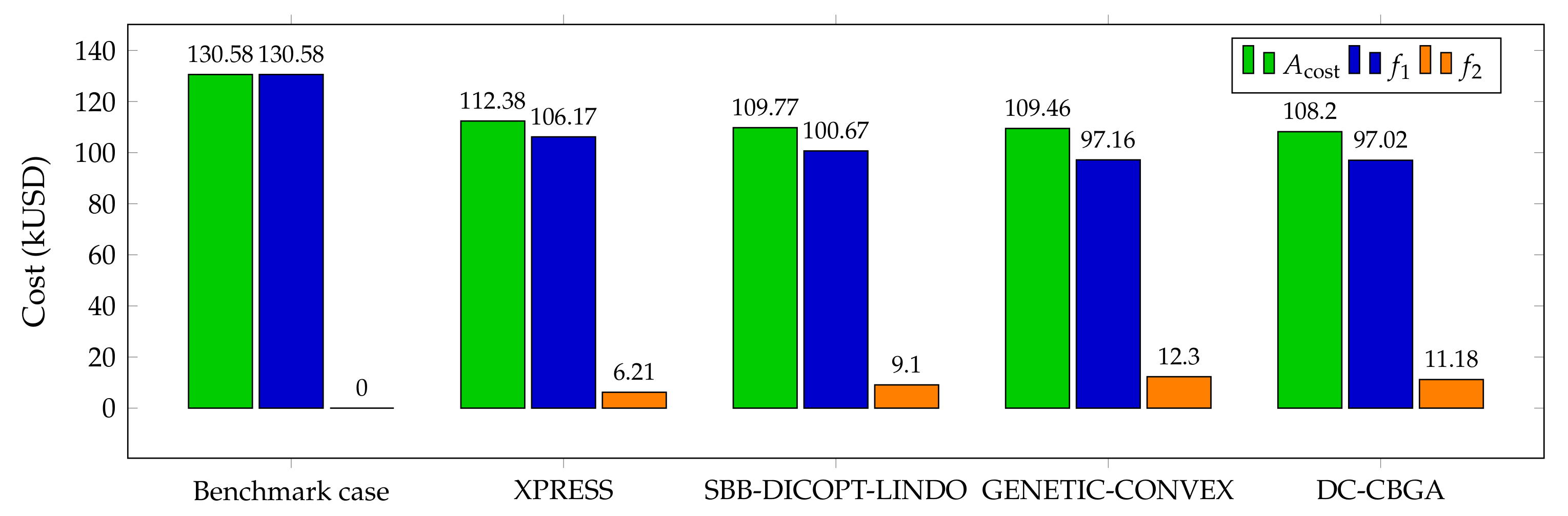
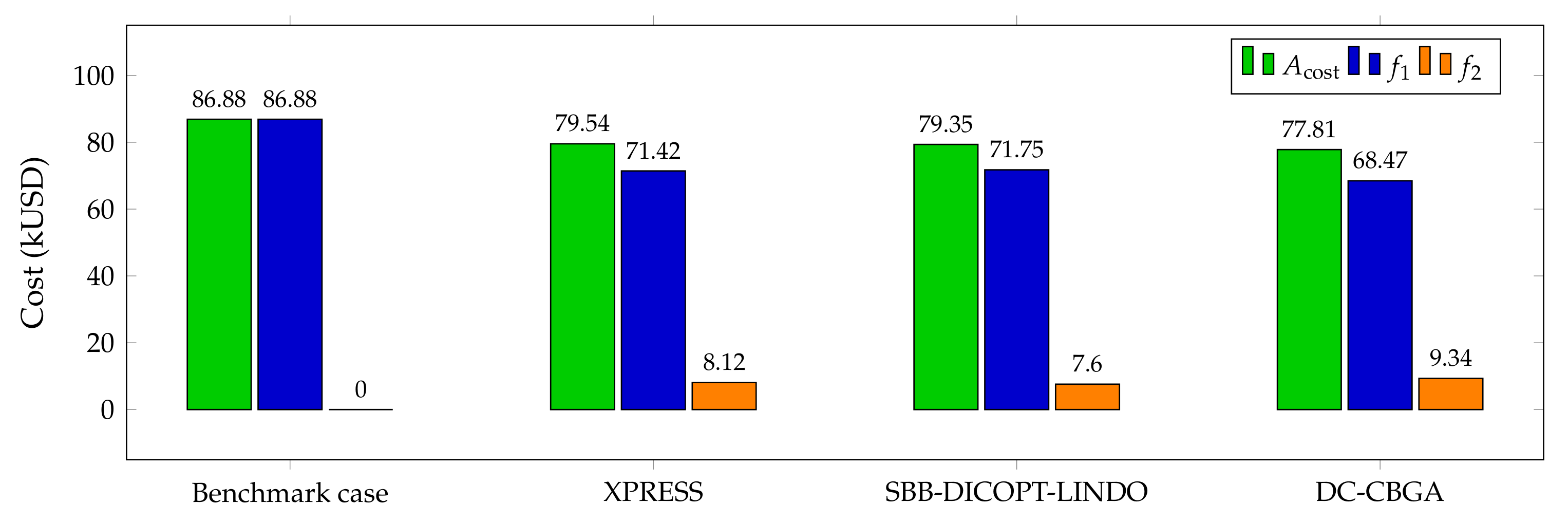
The results obtained show that with a population size of 20 individuals, DC-CBGA finds the optimal solution. The radial and mesh configuration reduces the total annual operating costs of 17.14% and 10.44% through an approximate investment in D-STATCOM of US$11.180 and US$9.340 per year, respectively.

The DC-CBGA methodology achieved better results than the GAMS solvers: XPRESS, SBB, DICOPT, and LINDO for both radial and mesh configurations. In both cases, the GAMS solvers ended stuck in a locally optimal solution. This condition happens because these solvers have non-convex solution spaces, making their exploration difficult with exact optimization methodologies. In addition, the results obtained are compared with the Genetic-Convex method only for the radial configuration. The DC-CBGA methodology reduced energy loss costs by 140 USD with an investment in compensation systems of 1120 USD less than the Genetic-Convex methodology. Additionally, the DC-CBGA obtained processing times of approximately 26 min while the Genetic-Convex close to 3 h, showing a considerable reduction in these, considering that the computer equipment used has similar technical characteristics.

From this study, it will be possible to develop the following further studies: (i) include into the optimization problem the analysis of the uncertainties regarding demand curves or consider periods longer than one day to capture possible different load behaviors, for example, using some weeks or months; (ii) propose a unified optimization methodology based on mixed-integer convex optimization that allows reaching the global optimum of the problem of the optimal location and sizing of D-STATCOM in distribution networks with radial or meshed configurations; (iii) evaluate the effects of the installation of D-STATCOM in three-phase networks with relevant load imbalances.

References

1. Cavellucci, C.; Lyra, C. Minimization of Energy Losses in Electric Power Distribution Systems by Intelligent Search Strategies. IFAC Proc. Vol. 1995, 28, 589–594. [Google Scholar] [CrossRef]
2. Montoya, O.D.; Gil-González, W.; Hernández, J.C. Efficient Operative Cost Reduction in Distribution Grids Considering the Optimal Placement and Sizing of D-STATCOMs Using a Discrete-Continuous VSA. Appl. Sci. 2021, 11, 2175. [Google Scholar] [CrossRef]
3. Alam, M.S.; Arefifar, S.A. Energy Management in Power Distribution Systems: Review, Classification, Limitations and Challenges. IEEE Access 2019, 7, 92979–93001. [Google Scholar] [CrossRef]
4. Sadovskaia, K.; Bogdanov, D.; Honkapuro, S.; Breyer, C. Power transmission and distribution losses—A model based on available empirical data and future trends for all countries globally. Int. J. Electr. Power Energy Syst. 2019, 107, 98–109. [Google Scholar] [CrossRef]
5. Comisión de Regulación de Energía y Gas. CREG. Resolución CREG 119 de 21 de Diciembre de 2007; CREG: Bogotá, Colombia, 2007. [Google Scholar]
6. Colmenar-Santos, A.; Reino-Rio, C.; Borge-Diez, D.; Collado-Fernández, E. Distributed generation: A review of factors that can contribute most to achieve a scenario of DG units embedded in the new distribution networks. Renew. Sustain. Energy Rev. 2016, 59, 1130–1148. [Google Scholar] [CrossRef]
7. Muruganantham, B.; Selvam, M.M.; Gnanadass, R.; Padhy, N.P. Energy loss reduction and load balancing through network reconfiguration in practical LV distribution feeder using GAMS. In Proceedings of the 7th International Conference on Power Systems (ICPS), Pune, India, 21–23 December 2017; IEEE: Piscataway, NJ, USA, 2017. [Google Scholar] [CrossRef]
8. Elsheikh, A.; Helmy, Y.; Abouelseoud, Y.; Elsherif, A. Optimal capacitor placement and sizing in radial electric power systems. Alex. Eng. J. 2014, 53, 809–816. [Google Scholar] [CrossRef] [Green Version]
9. Tamilselvan, V.; Jayabarathi, T.; Raghunathan, T.; Yang, X.S. Optimal capacitor placement in radial distribution systems using flower pollination algorithm. Alex. Eng. J. 2018, 57, 2775–2786. [Google Scholar] [CrossRef]
10. Sirjani, R.; Jordehi, A.R. Optimal placement and sizing of distribution static compensator (D-STATCOM) in electric distribution networks: A review. Renew. Sustain. Energy Rev. 2017, 77, 688–694. [Google Scholar] [CrossRef]
11. Montoya, O.D.; Chamorro, H.R.; Alvarado-Barrios, L.; Gil-González, W.; Orozco-Henao, C. Genetic-Convex Model for Dynamic Reactive Power Compensation in Distribution Networks Using D-STATCOMs. Appl. Sci. 2021, 11, 3353. [Google Scholar] [CrossRef]
12. Sedighizadeh, M.; Eisapour-Moarref, A. The Imperialist Competitive Algorithm for Optimal Multi-Objective Location and Sizing of DSTATCOM in Distribution Systems Considering Loads Uncertainty. INAE Lett. 2017, 2, 83–95. [Google Scholar] [CrossRef] [Green Version]
13. Zhang, Q.; Chen, H.; Luo, J.; Xu, Y.; Wu, C.; Li, C. Chaos Enhanced Bacterial Foraging Optimization for Global Optimization. IEEE Access 2018, 6, 64905–64919. [Google Scholar] [CrossRef]
14. Yuvaraj, T.; Devabalaji, K.; Ravi, K. Optimal Placement and Sizing of DSTATCOM Using Harmony Search Algorithm. Energy Procedia 2015, 79, 759–765. [Google Scholar] [CrossRef] [Green Version]
15. Taher, S.A.; Afsari, S.A. Optimal location and sizing of DSTATCOM in distribution systems by immune algorithm. Int. J. Electr. Power Energy Syst. 2014, 60, 34–44. [Google Scholar] [CrossRef]
16. Marjani, S.R.; Talavat, V.; Galvani, S. Optimal allocation of D-STATCOM and reconfiguration in radial distribution network using MOPSO algorithm in TOPSIS framework. Int. Trans. Electr. Energy Syst. 2018, 29, e2723. [Google Scholar] [CrossRef]
17. Tolabi, H.B.; Ali, M.H.; Rizwan, M. Simultaneous Reconfiguration, Optimal Placement of DSTATCOM, and Photovoltaic Array in a Distribution System Based on Fuzzy-ACO Approach. IEEE Trans. Sustain. Energy 2015, 6, 210–218. [Google Scholar] [CrossRef]
18. Gupta, A.R.; Kumar, A. Energy Savings Using D-STATCOM Placement in Radial Distribution System; Elsevier: Amsterdam, The Netherlands, 2015; Volume 70, pp. 558–564. [Google Scholar] [CrossRef] [Green Version]
19. Rukmani, D.K.; Thangaraj, Y.; Subramaniam, U.; Ramachandran, S.; Elavarasan, R.M.; Das, N.; Baringo, L.; Rasheed, M.I.A. A New Approach to Optimal Location and Sizing of DSTATCOM in Radial Distribution Networks Using Bio-Inspired Cuckoo Search Algorithm. Energies 2020, 13, 4615. [Google Scholar] [CrossRef]
20. Samimi, A.; Golkar, M.A. A Novel Method for Optimal Placement of STATCOM in Distribution Networks Using Sensitivity Analysis by DIgSILENT Software. In Proceedings of the 2011 Asia-Pacific Power and Energy Engineering Conference, Wuhan, China, 25–28 March 2011; pp. 1–5. [Google Scholar] [CrossRef]
21. Muthukumar, K.; Jayalalitha, S. Optimal placement and sizing of distributed generators and shunt capacitors for power loss minimization in radial distribution networks using hybrid heuristic search optimization technique. Int. J. Electr. Power Energy Syst. 2016, 78, 299–319. [Google Scholar] [CrossRef]
22. Sannigrahi, S.; Acharjee, P. Implementation of crow search algorithm for optimal allocation of DG and DSTATCOM in practical distribution system. In Proceedings of the 2018 International Conference on Power, Instrumentation, Control and Computing (PICC), Thrissur, India, 18–20 January 2018; IEEE: Piscataway, NJ, USA, 2018. [Google Scholar] [CrossRef]
23. Rajan, C.S.G.; Ravi, K. Optimal placement and sizing of DSTATCOM using Ant lion optimization algorithm. In Proceedings of the 2019 International Conference on Computation of Power, Energy, Information and Communication (ICCPEIC), Melmaruvathur, India, 27–28 March 2019; IEEE: Piscataway, NJ, USA, 2019. [Google Scholar] [CrossRef]
24. Amin, A.; Kamel, S.; Selim, A.; Nasrat, L. Optimal Placement of Distribution Static Compensators in Radial Distribution Systems Using Hybrid Analytical-Coyote optimization Technique. In Proceedings of the 2019 21st International Middle East Power Systems Conference (MEPCON), Cairo, Egypt, 17–19 December 2019; IEEE: Piscataway, NJ, USA, 2019. [Google Scholar] [CrossRef]
25. Dash, S.; Mishra, S. Simultaneous Optimal Placement and Sizing of D- STATCOMs Using a Modified Sine Cosine Algorithm. In Advances in Intelligent Computing and Communication; Springer: Singapore, 2020. [Google Scholar]
26. Montoya, O.D.; Fuentes, J.E.; Moya, F.D.; Barrios, J.Á.; Chamorro, H.R. Reduction of Annual Operational Costs in Power Systems through the Optimal Siting and Sizing of STATCOMs. Appl. Sci. 2021, 11, 4634. [Google Scholar] [CrossRef]
27. Huanca, D.; Gallego, L. Chu and Beasley Genetic Algorithm to Solve the Transmission Network Expansion Planning Problem Considering Active Power Losses. IEEE Latin Am. Trans. 2021, 19, 1967–1975. [Google Scholar]
28. Comisión de Regulación De Energía y Gas. CREG. RESOLUCIÓN No. 024 de 2005; CREG: Bogotá, Colombia, 2005. [Google Scholar]
29. Montoya, O.D.; Gil-González, W.; Giral, D.A. On the Matricial Formulation of Iterative Sweep Power Flow for Radial and Meshed Distribution Networks with Guarantee of Convergence. Appl. Sci. 2020, 10, 5802. [Google Scholar] [CrossRef]
30. Shen, T.; Li, Y.; Xiang, J. A Graph-Based Power Flow Method for Balanced Distribution Systems. Energies 2018, 11, 511. [Google Scholar] [CrossRef] [Green Version]
31. Vasconcellos, D.B.; González, P.P.; González, G.F. Control de demanda eléctrica aplicando algoritmos genéticos. Ingeniare Rev. Chilena de Ingeniería 2017, 25, 389–398. [Google Scholar] [CrossRef] [Green Version]
32. Zhao, J.-Q.; Wang, L. Center Based Genetic Algorithm and its application to the stiffness equivalence of the aircraft wing. Expert Syst. Appl. 2011, 38, 6254–6261. [Google Scholar] [CrossRef]
33. Duan, D.L.; Ling, X.D.; Wu, X.Y.; Zhong, B. Reconfiguration of distribution network for loss reduction and reliability improvement based on an enhanced genetic algorithm. Int. J. Electr. Power Energy Syst. 2015, 64, 88–95. [Google Scholar] [CrossRef]
34. Singh, B.; Singh, S. GA-based optimization for integration of DGs, STATCOM and PHEVs in distribution systems. Energy Rep. 2019, 5, 84–103. [Google Scholar] [CrossRef]
35. Venkatesh, B.; Ranjan, R. Optimal radial distribution system reconfiguration using fuzzy adaptation of evolutionary programming. Int. J. Electr. Power Energy Syst. 2003, 25, 775–780. [Google Scholar] [CrossRef]
Figure 1. Flow chart for the proposed master–slave solution methodology.
Electronics 10 01452 g001
Figure 2. IEEE 33-bus network.
Electronics 10 01452 g002
Figure 3. Load curves: residential, commercial, and industrial.
Electronics 10 01452 g003
Figure 4. Operating costs discriminated into investment costs and loss costs for the methodologies used in the radial configuration.
Electronics 10 01452 g004
Figure 5. Operating costs discriminated into investment costs and costs for losses for the methodologies used in the mesh configuration.
Electronics 10 01452 g005