Lyapunov Based Reference Model of Tension Control in a Continuous Strip Processing Line with Multi-Motor Drive


1
Department of Electrical Engineering and Mechatronics, FEI TU of Košice, Letná 9, 042 00 Košice, Slovakia
2
Department of Energy Technology, Aalborg University, 6700 Esbjerg, Denmark
*
Author to whom correspondence should be addressed.
Electronics 2019, 8(1), 60; https://doi.org/10.3390/electronics8010060
Submission received: 20 November 2018
/
Revised: 21 December 2018
/
Accepted: 26 December 2018
/
Published: 4 January 2019
(This article belongs to the Special Issue Renewable Electric Energy Systems)
Abstract
:The article describes design and experimental verification of a new control structure with reference model for a multi-motor drive of a continuous technological line in which the motors are mutually mechanically coupled through processed material. Its principle consists in creating an additional information by introducing a new suitable state variable into the system. This helps to achieve a zero steady-state control deviation of the tension in the strip. Afterwards, the tension controller is designed to ensure asymptotic stability of the extended system by applying the second Lyapunov method. The realized experimental measurements performed on a continuous line laboratory model confirm the advantages and correctness of the proposed control structure: it is simple, stable, robust against changes of parameters, invariant to operating disturbances and ensures a high-quality dynamics of the controlled system prescribed by the reference model. To demonstrate effectiveness of the design, the performance of the controller was compared with properties of a standard Proportional Integral Derivative/Proportional Integral (PID/PI) controller designed in frequency domain.
1. Introduction
Multi-motor motor drive of a continuous technological line for production and processing of strips of various materials (metal, paper, plastic, etc.) in various profiles (strips, tubes, foils, etc.) presents a complex and coupled multi-input multi-output (MIMO) nonlinear system. Here, the drives are mutually mechanically coupled by the processed material which influences behaviour of the drives (torque, speed), esp. in dynamical states. From technological point of view, the tension in the material within an area of elastic deformations causes changes in its internal structure by appropriate rearrangement of the material elementary particles and hence the material obtains new mechanical properties. Thus the quality of the strip exiting from the line depends on quality of the tension control system which should keep the constant tension in the strip regardless variations of the strip speed, external disturbances and variations of the system parameters. The system control should ensure constant and nonoscillating tensions in the strip in sections among processing machines during all operation states and regardless of any change of parameters of the system (e.g., moment of inertia).
The central (i.e., technological) section (CS) of the continuous line (CL) is the object of our research. Here, the basic requirement consists in control of the strip tension during all line operating states—starting, running-up, stopping, regardless of disturbances in the strip tension and change of mechanical parameters (e.g., moment of inertia, etc.), while the material should run at the prescribed constant line speed. This leads to necessity of high quality tension control of a nonlinear system with inaccurately known parameters and external additive disturbances, independently of its speed [1,2,3].
The objectives of the control goals are summarized as follows:
- Autonomous (decoupled) control of controlled variables of CL (tension and speed values).
- Invariance against additive disturbances.
- Robustness against changes of important line parameters (change of the processed material and its dimensions which cause change of damping constant and constant of elasticity and change of the moment of inertia of the drive).
- Required dynamics of the controlled variable (time courses of tensions in line sections without any overshoots).
- Stability of the controlled system.
Linear control methods are able to ensure invariance of the system against disturbances but they are inapplicable for synthesis of controllers of nonlinear MIMO systems. These methods do not ensure desired robustness and decoupled control, especially in dynamic states. For example, due to insufficient decoupling at changed parameters, a rapid change in the line speed may result in undesired tensions causing deformation of the strip and even could lead to strip disruption [4].
In recent years, many different control methods have been proposed and applied to tension control in CL [5]. Since the model of CL consists of several interconnected subsystems that are mutually influence themselves, the use of decentralized control structures is justified and often used, primarily due to using simple PID or PI controllers [6,7,8,9,10,11]. Methods of their design are simple, but arising interconnections between the speed and tension subsystems represent a significant limitation in technological line operation, especially in dynamic states. To avoid this, correction couplings are used, but they have more or less complex transfer functions.
Optimal control methods for MIMO systems [12,13,14,15,16,17] reduce impact of the described mutual interactions but they usually require knowledge of a precise model and parameters of the controlled system. A very important aspect at design of these controllers is presence of various external disturbances which can cause deterioration of the quality and even destruction of the processed strip [4]. Therefore, the control strategy should be enough robust to eliminate these failures.
To control the tension in the Central Section Continuous Line (CSCL), robust control structures providing stability and invariance against the disturbances have been proposed, but the robustness is often ensured only within a narrow range of changes of parameters [18,19,20,21,22,23], while using relatively complex correction couplings [24,25]. Advanced control methods, such as feedback control using observers [26,27,28], time-optimal control [29], and H-infinity control [30,31] are methods that achieve relatively good control performance but they are too complex in terms of structure and design of parameters of the controllers and this presents their main disadvantage in their wider implementation in industrial practice.
For control of nonlinear MIMO systems, intelligent control methods, especially those based on fuzzy logic, are also used. For example, for control of a CL, classical fuzzy logic controllers are designed on basis of linguistic rules based on expert experience [32,33,34,35,36]. Their main disadvantage dwells in the fact that there do not exist standard methods for transforming human knowledge base into fuzzy rules. An optimal PI controller based on a fuzzy model of CL [37] was also designed, but its quality depends strongly on quality and properties of the designed fuzzy model. The fuzzy model is obtained from experimental measurements of I/O functions and the obtained database should be consistent covering entire workspace of the control system. This is relatively complicated and time-consuming task. In addition, the operation of fuzzy controllers in boundary states very often leads to problems with the dynamics and stability of control and the application of fuzzy control methods is also difficult to understand and thus difficult to implement widely in common industrial practice.
Since the multi-motor drives are used in larger technological units, it is necessary to look for such methods of their control that would be simple and physically easy interpreted at providing all required control features such as decoupling, required dynamics, stability, invariance and robustness. Otherwise, they have not any chance to be widely used in industrial practice.
One way to achieve these goals consists in using control structures with a reference model designed on a basis of the second Lyapunov method. This method can also be applicable for MIMO systems [38,39,40,41]. Such control structures allow, that a general nonlinear time-variant continuous system would reach a defined stable steady state when using the prescribed reference model. The complexity of the structure of the proposed controllers depends on a suitable choice of the Lyapunov function [42,43,44,45]. Because the process of designing the control structures according to this method has some optional elements, there are generally many variations of such structures that are derived from the method.
In this article, a new robust control structure with a reference model whose stability is derived on basis of the second Lyapunov method [46] is designed to control the tension in the strip running in a line section between two work (or transport) rolls. This simplified system is used for the following reason: the designed structure has optimal dynamic properties in terms of the minimum control deviation and minimum input energy [47] criteria, which are normally used in control circuits. The main idea of the proposed method consists in extending the system control algorithm by a new additional information that can be easily obtained from the system output quantity that ensures the zero steady state value of the output variable. If for this extended system a control algorithm is designed ensuring asymptotic stability of the system and prescribed dynamics according to the reference model, it will automatically reach the goal of control both in the steady-state and in the transient state.
The properties of the novel control structure have been verified by experimental measurements on a continuous line laboratory model. The obtained results are compared with properties of a MIMO PID/PI controller designed for the speed and tension control of a CSCL. However, in the case of MIMO controllers, it is necessary to design corrective couplings with corresponding transfer functions that ensure decoupling of the speed and tension transfer channels.
2. Continuous Line Model
2.1. Continuous Line Description
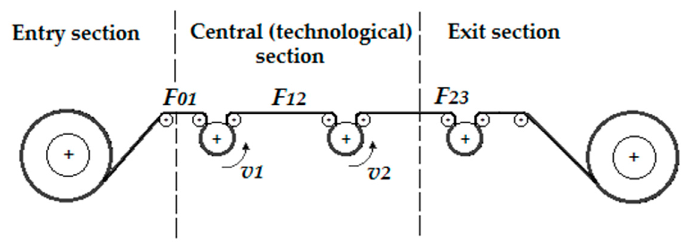
A CL generally consists of three sections [4]:
- The entry section consisting of un-coiler, strip linking machine and entry accumulator serving for accumulation of a stock of material for the technological section and sometimes also for reduction of tension in the strip (between the uncoiler and the following part of the line).
- The central (technological section), where technological operations are carried out according to the technological prescription for the particular material.
- The exit section consisting of coiler for coiling of the strip materials (including also exit accumulator and strip divider).
In industry there exists various typical multi-motor drive configurations of CSCL [4]. The tension in the strip arises due to different circumferential speeds of the work rolls in the line section. For the sake of simplicity, the coupling of only a two-motor drive is investigated here but the proposed idea can be extended to an indefinite number of machines coupled by processed material. Thus, in CL, with more sections it is possible to control the strip tension individually in each section of the line.
In our case, two DC motors of a considered CSCL are supplied by power electronic converters (TC, Figure 1) through the gear with the gear ratio j. Here F12 is the tension in the strip and v1, v2 are circumferential speeds of the machine rolls. In the considered arrangement the tension in the precedent section and in the section following the considered section line present main disturbances which affect the load torques of the first and of the second drives. In Figure 1 KF is the tension sensor, Kv is the circumferential speed sensor (considering , where r is roll radius and is motor angular speed), uF12 is the output voltage of the tension sensor and uv1, uv2 are output voltages from the speed sensors.
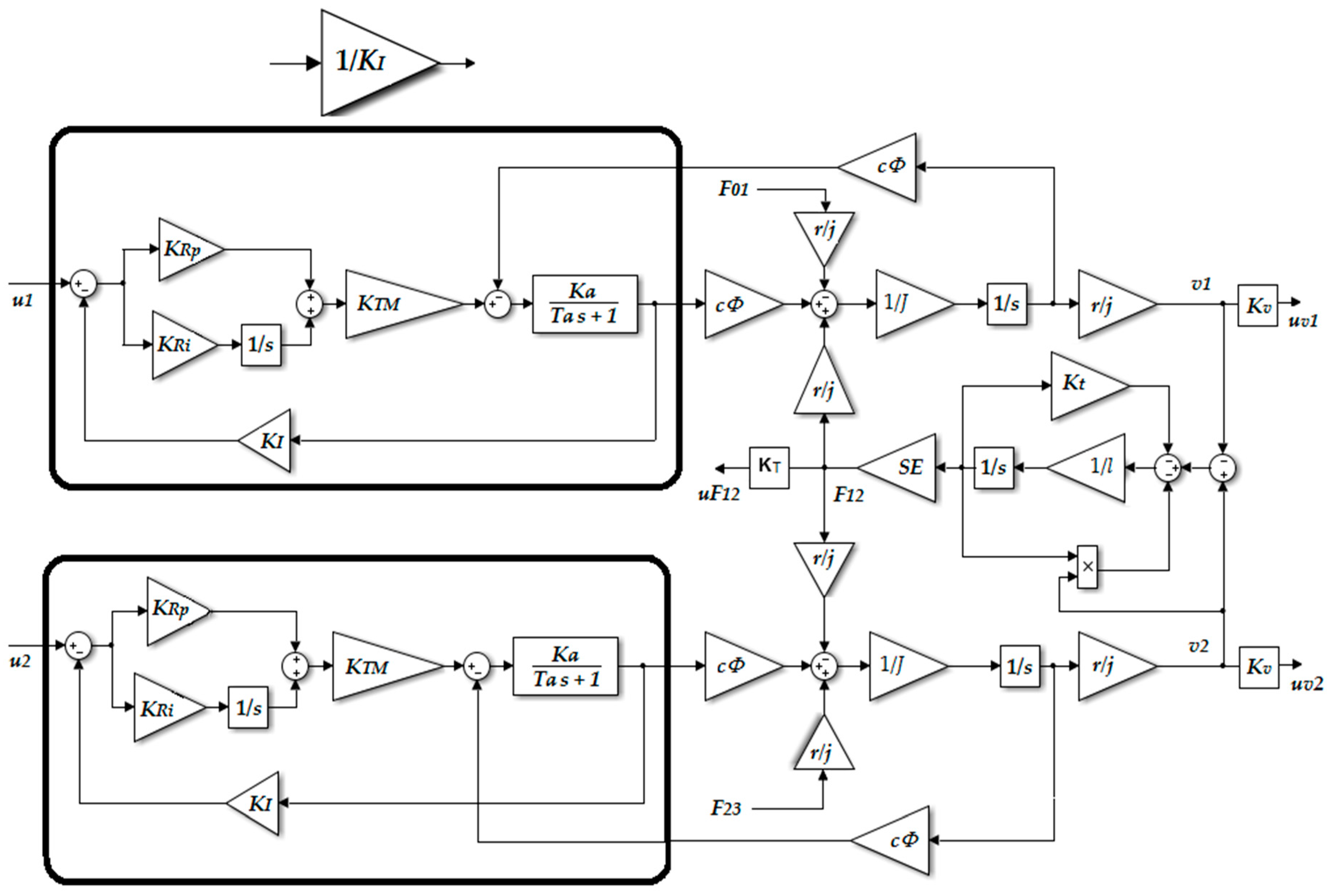
The corresponding block diagram is shown in Figure 2. The elastic coupling is modelled according to Brandenburg [48,49,50], taking into consideration variable time mechanical constant of the running elastic strip depending on the strip speed which makes the model nonlinear. In Figure 2, l is distance between the rollers of the work machines, S—the cross-section of the processed material, E represents the Young modulus of elasticity, Kt—material damping constant, KT—gain of the tension sensor, J—total moment of inertia on the motor shaft (let us consider for sake of simplicity that both motors and work machines are similar) and cΦ—torque constant of the motor.
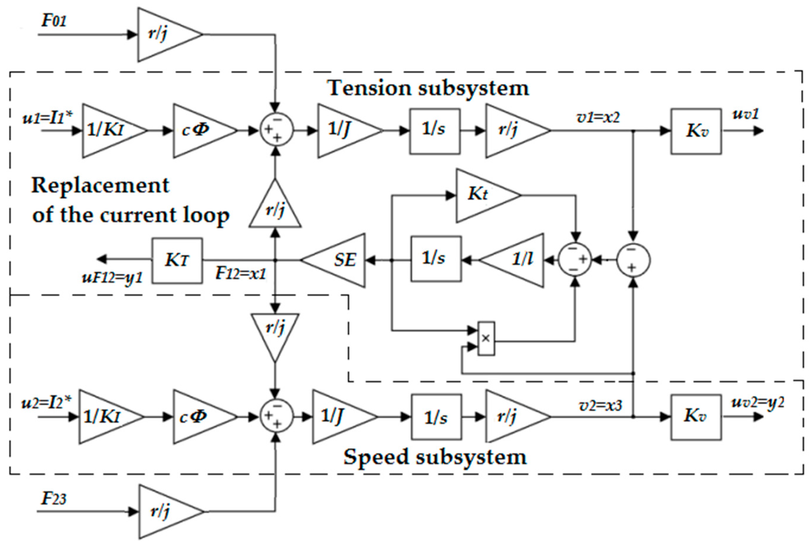
The power converters (TC) have proportional gain KTM and built-in fast current control loops with current controllers of the PI type having parameters KRp (proportional gain) and KRi (integral gain). If the mechanical time constant of the drive is much greater than the electrical time constant of the motor, neglected can be the dynamics of the current loop (the box marked by a thick line in Figure 2) and the motor emf. By such simplification, the current loop can be replaced with satisfactory precision by the transfer function 1/KI (marked in Figure 2) where KI is the current sensor gain. By such simplification the current references ( and ) present inputs into CSCL model. The block diagram with the described simplification is shown in Figure 3.
2.2. Mathematical Model of a Part of a Continuous Line with Two Machines
The analytical design of the Lyapunov-based model reference tension control in CSCL starts from a mathematical description of the electromechanical system. From the control point of view, the CSCL presents a multivariable nonlinear MIMO system of the third order with two inputs (u1 = , u2 = ), two outputs (y1 = uF12; y2 = uv2), and two additive disturbances (F01, F23), which represent tensions in the previous () and the following () sections of the considered part of the CSCL. In the block diagram in Figure 3, the state variables were chosen as follows: x1 = F12, x2 = v1, and x3 = v2, i.e., the vectors are:
The general form of state-space description of the dynamical system is:
In the block diagram in Figure 3 the elements of the matrix C present gains of sensors of output quantities, E is disturbance matrix, and D is zero matrix.
Note: numerical values of matrices for the line parameters in considered model of the line are listed the Appendix A.
2.3. Analysis of Properties of the Central Section of the Continuous Line
To determine basic properties of CSCL, experimental identification measurements were made on the laboratory model described in Section 4.1 for current pulses applied sequentially to each input of the model that are shown in Figure 4: the reference signals of —the first motor current and —the second one. The calculations were performed with a sampling time of 1 ms, and the outputs are plotted in the graph.
From the time courses in Figure 4b it is seen that the system contains a fast (tension) subsystem with oscillating response and a slow (speed) subsystem. They are coupled and mutually interact. From the physical analysis of the continuous line model [4,13], it follows that change of the strip speed or change of properties of the processed strip material cause change of the controlled system dynamics. In such a MIMO system, a strong interaction between the transfer channels of the tension and of the speed leads to worsening of the strip quality, even can lead to destruction of the processed strip.
3. Design of a Control Structure with Reference Model for the Central Section of a Continuous Line
3.1. Mathematical Model of the Tension Subsystem
From point of view of control, the tension subsystem (marked by dashed line in Figure 3) presents the second order system with one input u1 = and one output variable y1 = uF12. Regarding the tension control (where the tension is controlled by the first drive, i.e., by the input u1), the input u2 in the diagram in Figure 3 is understood as a slowly changing external disturbance. In our notation the first state variable presents the tension (x1 = F12 = xT1 and the second one is the circumferential speed of the first work rolls (x2 = v1 = xT1), where from view of the tension control the speed of the output strip v2 is considered as an additive external disturbance. Here the index T denotes variables of the tension subsystem. The disturbance vector fT for the tension subsystem, consisting of the tension F01 in the strip inputting into the considered line section and of the circumferential speed of the second work rolls v2, presents another additive disturbance to the disturbance F23 (which is the tension of the outputting strip, behind the second work rolls).
The state equations of the tension subsystem are similar to Equations (2) and (3):
where now the vectors have the notation:
The matrices of the state-space model of the tensions subsystem of the 2nd order are in the form:
3.2. Reference Model Design
The required dynamic properties of CL will be influenced by a suitable reference model. It is suitable to choose this model as a linear system, because it can be optimally designed using known methods of optimal control theory and generally it is of the same order as the controlled system. Let us select the reference model for our controlled system in the state-space form:
where AM is the state matrix of the reference model, BM is the reference model input matrix, xM is the state vector of the reference model, and w is the setpoint (the index M denotes the reference model variables).
Since it is intended to obtain additional information about unknown parametric and additive disturbances for a controlled second order system, the reference model will be extended by a new state variable xM3 = xMe (the index e—extended) ensuring that the tension deviation is equal to zero in the steady state. According to [47] a linear system of the third order has been chosen as the reference model. Its dynamics is adjustable by the only optional positive parameter α. Such reference model is able to provide the optimal dynamic properties of the controlled system in accordance with the criteria of minimum regulatory deviation criterion and minimum input energy.
The block diagram of the third order reference model under consideration is shown in Figure 5, where in steady state the input of the integrator xM3 is equal to zero and the tension is equal to the reference value w = uF12* (the asterisk * denotes the required value).
The augmented state description of the reference model for the third order system in Figure 5 is in the form:
which in our case according to [47] is:
Note: In the present consideration the tension is generated by the first drive and the controlled strip speed is equal to the circumferential speed v2 of the work rollers driven by the second drive.
The optional positive parameter in the reference model α allows us to set the optimal dynamics of the controlled variable. The value of the parameter α is inversely proportional to the model dynamics; e.g., if we want to stabilize the tension in the strip material within time Ts = 1 s then on the basis of the Shannon–Kotelnik theorem , thus the value of the optional parameter is α = 1/T = 5.
3.3. Extended Tension Subsystem
The controlled system is described by the state Equations (2) and (3). From the point of view of the tension control, it presents a controlled system of the second order which, like the reference model, will be extended by the integrator of the output controlled variable. Its state description is:
where xTe is the added state variable and fTe is the disturbance acting upon this state variable.
Since the aim of controlling the electric drive is not to reach any zero state of the state vector x, but to reach the zero state of its control deviation from the set values, for the state vector components it is preferable to choose deviations of the state vector x from the desired values. The system stability will be also investigated with respect to these deviations.
If we introduce a deviation between the reference model and the controlled system in the form:
then by simple modifications we get a system whose states are represented by the state deviation e:
where we denoted:
which is a generalized disturbance vector including all parametric and additive disturbances acting on the system.
3.4. Principle of the Tension Controller Design by the Second Lyapunov Method
The aim of the controller design is to find such a mathematical formula for setting the input u that the zero solution of the system (25) would be asymptotically stable, i.e., , (the zero vector).
Generally, the Lyapunov function is most often chosen as a weighted quadratic form of system states because this is positively defined and simple. Let us choose the Lyapunov function for the system (25) in the form:
where:
is the weighted vector of deviations. The i-th element of this vector is in the form:
where pki are elements of a symmetric positively definite matrix P and n is order of the augmented system. The derivation of the Lyapunov function (27) considering the system (25) and with the vector bT according to the Equation (13) can be easy derived as follows:
The zero solution of the system (25) will be asymptotically stable if we ensure that the derivative of Lyapunov function (27) is negative definite. Then the following equation must be valid:
Equation (31) is the matrix Lyapunov equation, where P and Q are symmetric positive definite matrices.
By choice of the reference model according to Equation (10) we can avoid solving the Equation (31). According to the optimal control theory [47] for the state matrix of the reference model in the controllability form it is possible to determine the elements of the matrix P analytically and the following equation is valid:
Based on the above Equations (28), (31), (32) for the derivation of the Lyapunov function, we get:
where the positive definite matrix P, according to [45] is in the form of:
The specific elements of the matrix P in the Equation (36) are determined with regard to the desired dynamics of the controlled system prescribed by the reference model.
The first component on the right side in Equation (35) is always negative, because the expression eTz = eTPe, where z = Pe, is always positive. Then the system (25) will be asymptotically stable, i.e., its derivation will be negative, if for the input u it is valid:
where K is optional parameter. Its value we determine from the following consideration: the second component on the right side in the Equation (35) will be negative if the following inequality is met:
which can always be ensured by a sufficiently large value of the optional positive parameter K.
For creation of deviations of the state variables of the reference model and the system according to Equation (22), we can use the following arrangement:
CSCL as a controlled system described by the state, Equation (21) will then follow the reference model (Equation (19)) with , (the zero vector), i.e., the controlled system will be asymptotically stable if the input u1 is calculated according to Equation (37):
For the individual components of the vector z according to Equation (28) we can write
where the elements of the matrix P are determined by Equation (36).
The resulting block diagram of the tension control of CSCL is shown in Figure 6.
The tension control is decisive for the final product quality and thus, for controlling the speed of the CSCL (v2—circumferential speed of the work rolls driven by the second drive), an ordinary standard PI controller is used. As mentioned above, the change in speed v2 presents another additive disturbance for the proposed tension controller. PI speed controller parameters have been tuned using standard MATLAB tools, and its parameters are listed in the Appendix A.
4. Verification of the Designed Control Structure
4.1. Experimental Setup
Simulation results were verified by experimental measurements on a laboratory model of a continuous line that was built in the laboratory of the authors.
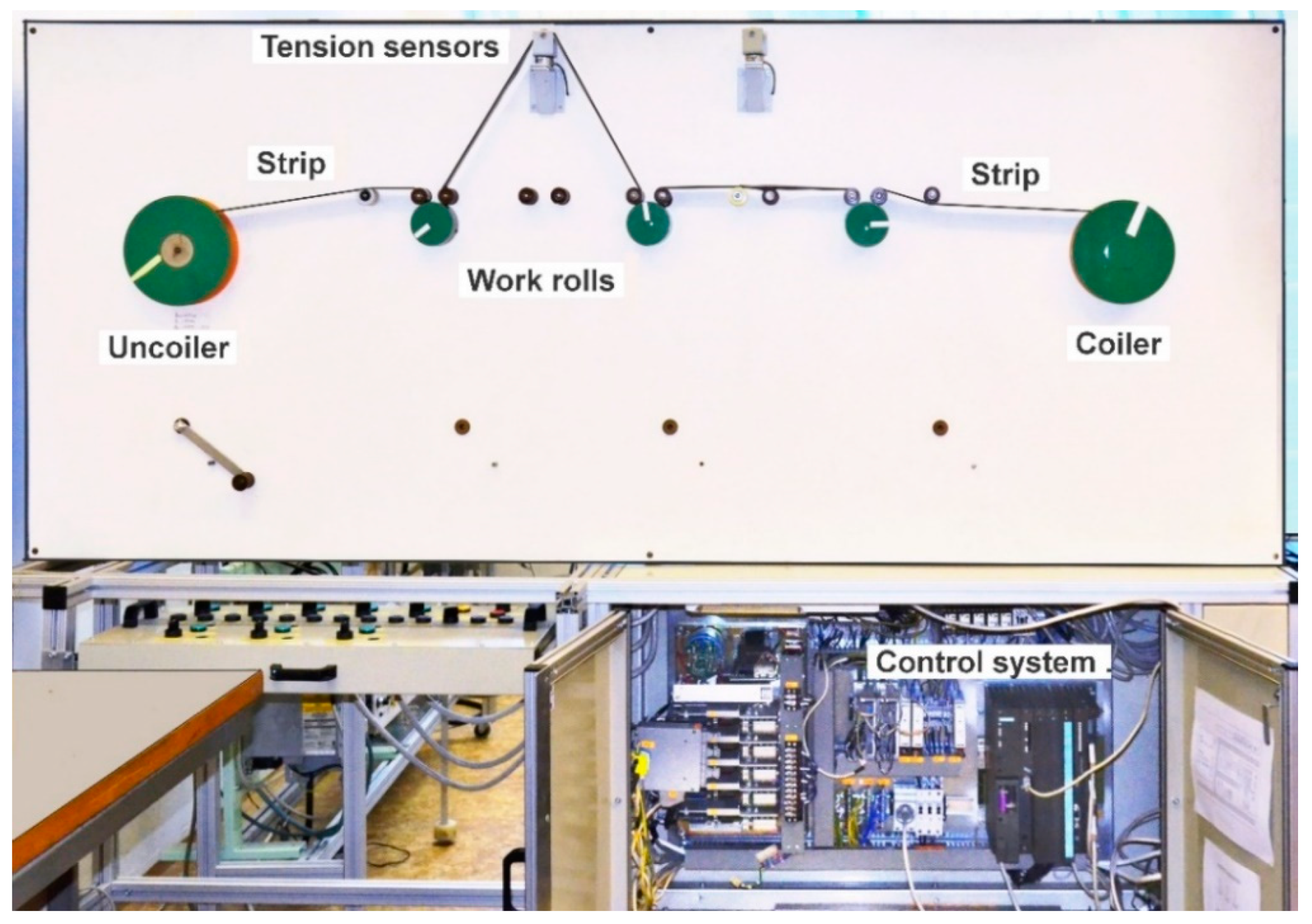
The laboratory model presents a functional model of a multi-motor drive with the sketch in Figure 7 where the drives are mutually coupled by a running strip of elastic material, which is a magnetic tape of the 0.03 m width. The strip, wound up into a coil, runs from the uncoiler to coiler, while its belt was around the three work rolls (in order to increase the friction surface between the strip and roll).
The model is driven by five Direct Current (DC) disc motors powered by Allen Bradley DC converters 1386 DC Servo Drive System with Pulse Width Modulation (PWM) modulation. The control system is based on a programmable controller PLC S7-400 with FM458 technological card. CFC language was used for the control program development. Controlling voltages for the converters within the range of ±10 V present inputs into the system and the speeds of the drives and tensions in the sections between the work rolls present outputs from the system. Incremental sensors (IRC) generating 4000 increments per revolution are used for measuring the revolutions of the motors. The tensions are sensed by two tension sensors. In our experiment to demonstrate the proposed control method we utilize the section with only two rolls and one tension sensor.
The CL laboratory model is shown in Figure 8. Its parameters used for calculation and simulation are specified in Appendix A.
4.2. Experimental Results
The features of the proposed control structure for the control of CSCL were verified in laboratory by experimental measurements on the described laboratory model. The operation cycle consists of three phases—starting the line, running at constant speed and stopping the line.
When verifying the properties of the proposed control, we have assumed that two types of external (additive) disturbances could occur, namely:
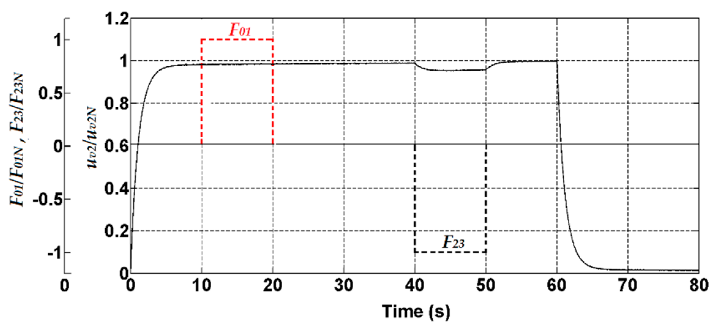
- Step changes of the tension before (F01) and after (F23) the considered line section with the amplitude of nominal tension at time t = 10 s and t = 40 s (Figure 9). In real line these disturbances are caused by sudden short changing the thickness in the material strip—when end of one strip is joined by welding to begin of other one.
- Slowly changing line speed v2, which is controlled by a standard PI controller. The time course of the strip speed v2 for the desired value equal to the nominal speed, i.e., for v2 = 0.6 ms−1, is shown in Figure 9 at simultaneous occurrence of the disturbances F01 and F23.
4.2.1. Experimental Results for the Designed Controller based on the Second Lyapunov Method
The proposed controller structure is based on the second Lyapunov method, which defines the range of its optional parameters, i.e., values of the elements of the matrix P and the positive optional parameter K for which the controlled system as a whole is stable. The elements of the matrix P are computed from the matrix Lyapunov Equation (31), where the positive definite matrix Q must be chosen. The values of elements of the matrix Q (and thus of the matrix P) influence the speed of declining the Lyapunov function (Equation [27]), which means a deceleration rate of the control deviation e. The system (25) will be stable for arbitrarily selected elements of the matrix Q when fulfilling the condition of its positive definiteness. However, if we choose the reference model to ensure the optimal dynamic properties of the controlled system according to the criterion of minimal control deviation and minimum input energy, then we can avoid solving the matrix Lyapunov Equation (27), because the elements of the matrix P can be determined analytically, based on Equation (32) from the matrix (36), as shown in Section 3.4.
The designed controlled structure also includes an optional parameter K in the Equation (40) for calculating the input u. This parameter must be positive and large enough to ensure asymptotic stability of the controlled system. On the other hand, the value of the parameter K is limited by physical constraints in the controlled system such as maximal current of electric motors, dynamics of real power converters, etc. The dynamic course of the output controlled variable—the tension F12 for the considered working cycle and for the parameter K = 2 is shown in Figure 10. It is obvious that the tension in CSCL practically monitors the reference tension prescribed by the reference model during the entire work cycle, even during the step disturbances F01 and F23 which act in time instants t = 10 s and t = 40 s, as shown in Figure 10. It is also observed on changes of the speed in Figure 9, which verifies the invariance of the proposed control against additive disturbances.
Due to the strong coupling between the strip speed and the web tension during normal operation cycle there exists many sources of disturbances, e.g., strip sliding along surface of the work roll or change of the material properties (i.e., the strip elasticity and damping). These disturbances influence the web tension and can lead to wrinkling or even breaking of the material. Therefore, the robustness during the entire operation cycle is an important target of the control strategy.
The robustness of the proposed control structure has been verified at change of two most important parameters of the controlled system that significantly affect properties of the elastic strip, namely the damping of the processed strip material (corresponding to changed material properties) and the moment of inertia of the drives. Figure 11 shows the time responses of the speed v2 and tension F12 when the damping constant of the material was decreased five times (i.e., five times more elastic material) and the moment of inertia was increased twice (the parameter K = 2).
Similarly, Figure 12 shows the dynamics of the speed and tension control when the damping of the strip material was increased five times and the moment inertia has been doubled (the parameter K = 2).
From the point of view of the real CL, there are significant and border changes in values of the parameters under consideration, while the dynamics, decoupling and invariance of the tension control remains virtually unchanged. This confirms the robustness of the proposed controller.
Experimental measurements have confirmed that the proposed controller is able to meet the basic control objectives, i.e., to predict the dynamics, invariance to external disturbances, robustness against changes of important parameters and this to ensure high quality material processing throughout the entire operation cycle (incl. the transient states).
4.2.2. Design of a CSCL Controller by MIMO System Design Method in Frequency Domain
In order to show the excellent properties of the proposed control structure with the reference model for control of CSCL, the obtained results are compared with those obtained when using the classical PID/PI controller for speed and tension control.
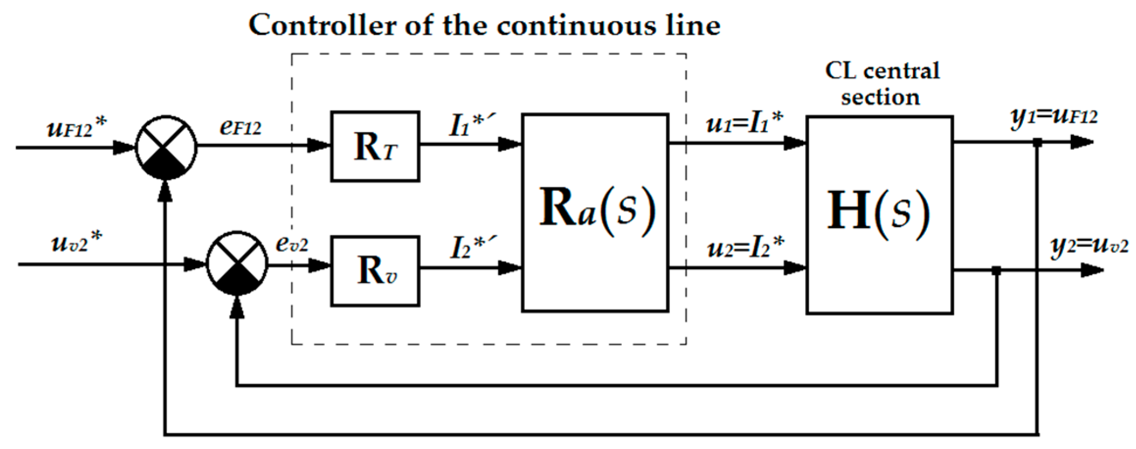
The overall block diagram of the standard control structure of the MIMO system in frequency domain is shown in Figure 13.
The design of the MIMO system control by standard methods is based on mathematical description of the controlled system by the matrix transfer function H(s), which describes the transfer functions among individual inputs and outputs of the MIMO system. This matrix is derived from the system mathematical description or can be computed, e.g., from matrices of the state-space model of the controlled system by the relationship:
Note: When calculating the H(s) matrix, we refer to CSCL as the third order system with the input, output and status variables as shown in Figure 3.
For each element of the transfer matrix H(s) it holds that:
and the transfer matrix H(s) for the parameters listed in the Appendix A is:
In the block diagram in Figure 13 the matrix Ra(s) is a matrix of decoupling controllers which ensure elimination of couplings between transfer channels of the tension and of the speed. From the point of view of a classic approach this means that for system decoupling in the open control circuit the following condition must be valid:
where the notation presents a diagonal matrix.
In our case, the controlled system described by the transfer matrix H(s) (46) has two cross couplings (transfer functions h12(s) and h21(s)) which must be compensated by the decoupling controller Ra(s):
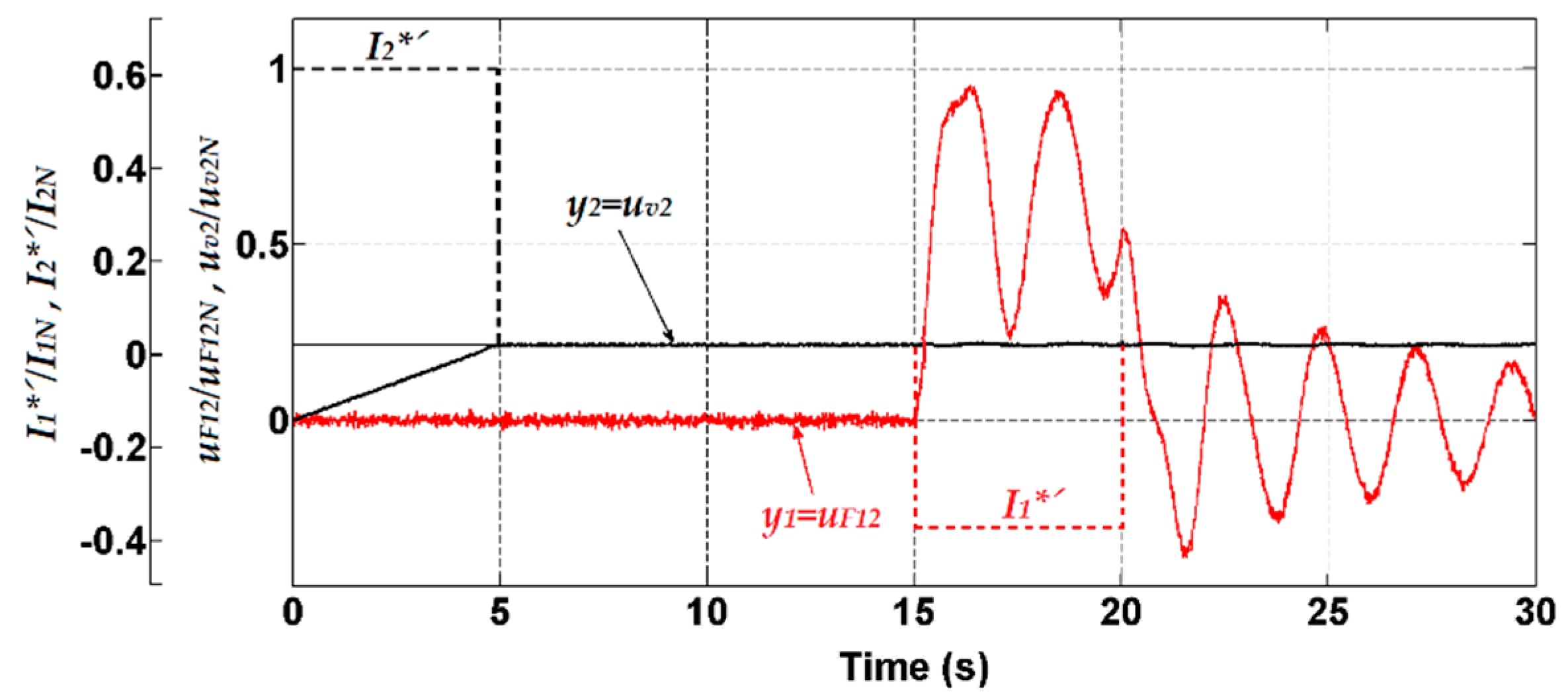
The achieved decoupling is demonstrated in the time responses shown in Figure 14. When changing the input only the output y2 = uv2 is changed, while the tension F12 remains unchanged and vice versa: when changing the input , only the output y1 = uF12 is changed and the speed v2 remains unchanged. The decoupling controller has transformed CL with two machines into two independent subsystems—a fast oscillating tension subsystem y1 = uF21 and a slow nonoscillating speed subsystem y2 = uv2.
For the speed and tension control it is possible to design by standard methods the PID-type controller for the tension subsystem and the PI type speed controller (Figure 15).
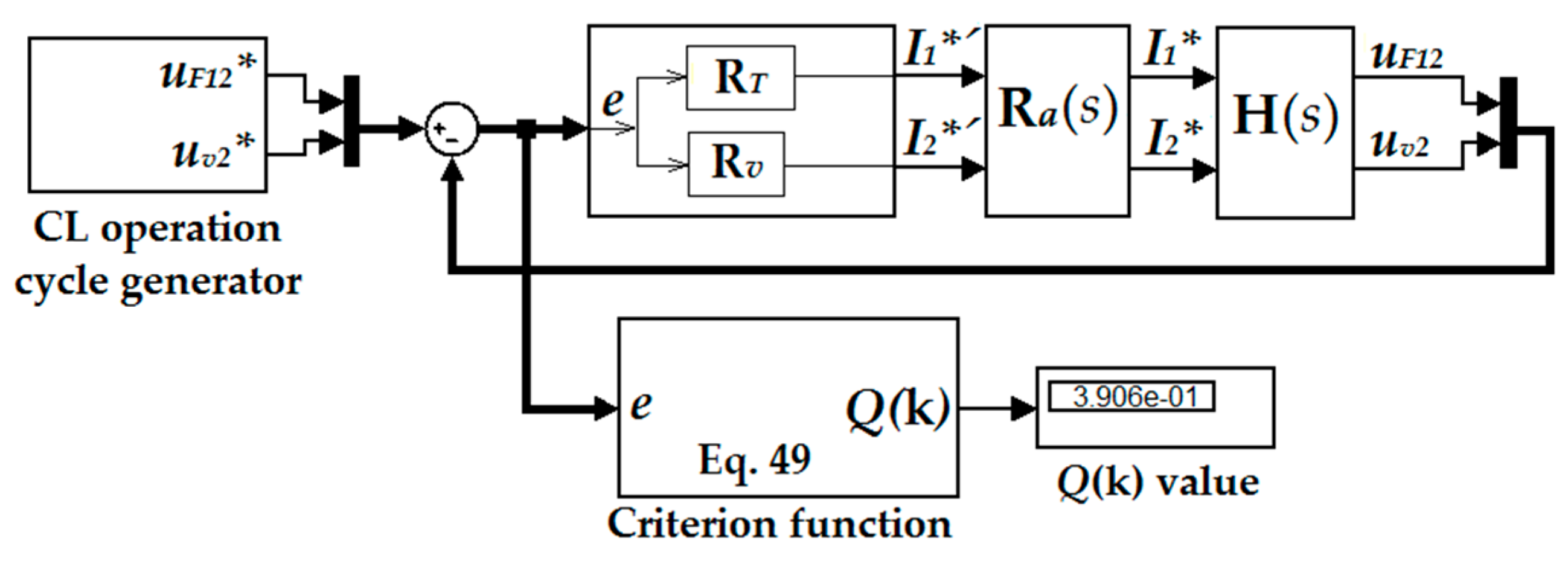
For such control structure, optimal parameters of the controllers were sought. The goal of the optimization consists in finding such vector of the controller parameters k = [KpF12 KiF12 KdF12 Kpv2 Kiv2]T so that the selected optimization criterion would be minimal. The optimization criterion was chosen in the quadratic form:
where e1 and e2 are the control deviations of the tension (uF12) and the strip speed (uv2) from the referenced values, and the coefficients C1 and C2 determine the weights (importance) that we confer to the individual output control deviations. In our case, we have chosen the values C1 = 5 and C2 = 1, which are physically interpreted as giving a stronger emphasis on quality of the tension control deviation e1 (i.e., to the tension in the material strip that primarily determines the quality of the output product). The optimal value of the parameters of the controller vector k is to be searched in the space of real values of gains of proportional, integration and derivation components.
It is a search of an extreme function of more variables, for which several methods of optimization are available (e.g., genetic algorithms, network charts, etc.). In our case, the method of uniform geometric partitioning of the parameter space into equal intervals and its systematic scan was chosen. This was realized by an m-file in MATLAB/Simulink environment (Figure 15). The advantage of this procedure is that the global minimum function (49) can be always found. The disadvantage consists in the time and computational difficulty if the vector k has more parameters and the division of the space is denser.
The algorithm of optimization works as follows: at the beginning of the optimization we chose the initial values of the controller parameters KpF120 = KiF120 = KdF120 = Kpv20 = Kiv20 = 1 (vector k0) and the space of parameters of particular controller gains is divided by the increments △KpF120 = 1, △KiF120 = 5, △KdF120 = 5, △Kpv20 = 1, △Kiv20 = 5. Maximum values for each parameter are defined: KpF12max = 50, KiF12max = 100, KdF12max = 100, Kpv2max = 50, Kiv2max = 100, according to the usual values of the proportional, integration and derivation components of the PID regulators The criteria function for initial values of the vector k0 and for the selected operation cycle of CL as specified in the Section 4.2 has a value Q(k0) = 37.19. After finding the optimal parameter vector kopt = [9, 20, 18, 7, 80]T, we obtained the value of the optimization criterion Q(kopt) = 0.3906.
4.2.3. Comparison of Results Obtained by Both Types of Controllers
The properties of both control structures, i.e.:
- The structure with the reference model structure and tension controller designed by the second Lyapunov method (having notation “Lyap” in time responses below).
- The structure with the speed and tension controllers designed in the frequency domain (notation and ) for the decoupled system, were compared for the reference values equal to the nominal tension and speed values, i.e., uF12 = 100% uF12N, uv2 = 100% uv2N, and with external additive disturbances, as shown in Figure 16.
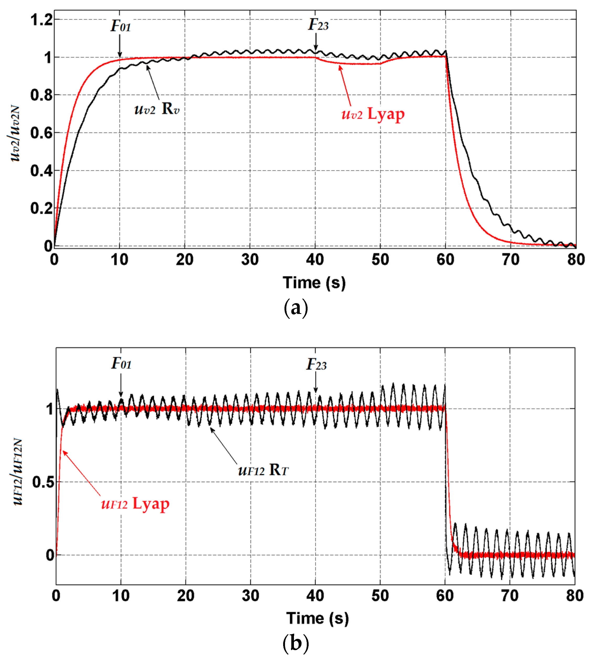
The degree of the robustness achieved for both control structures is shown in Figure 17 and holds for five times reduction in material damping and twice the increased moment of inertia of the drive.
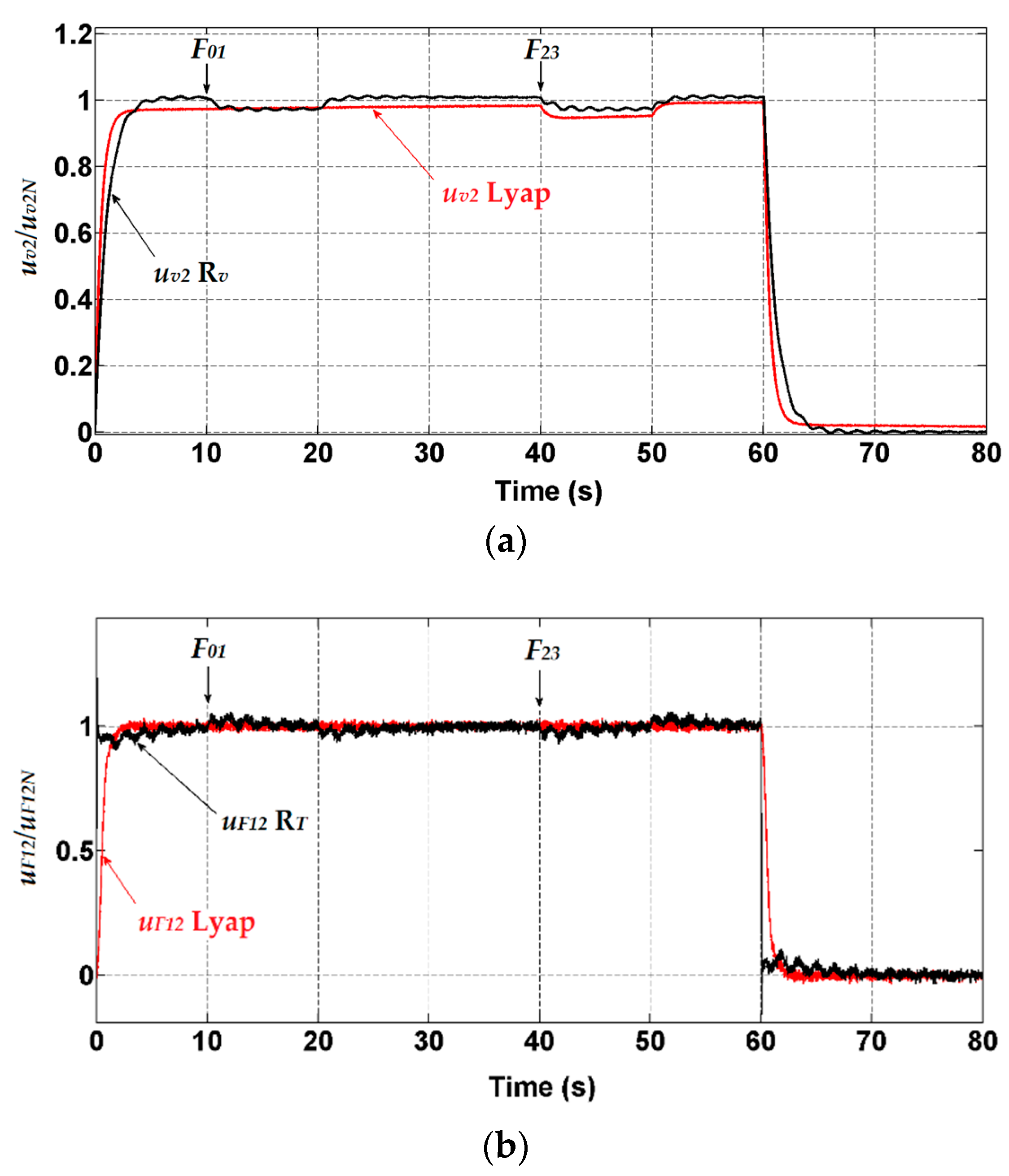
Similarly, the time responses in Figure 18 confirm the robustness of both control structures for the five-times increased damping of the material and twice-times the reduced moment of inertia of the drives. As mentioned above, this present a change of the material and machine important parameters which significantly affects the quality of the processed material.
5. Discussion of the Results
By comparing the above figures and based on the results obtained, we can say that both control structures are able to ensure the independent control of individual output variables: the speed and the tension in the CSCL. But the standard control structure with a PID tension controller and PI speed controllers showed a significant oscillation at occurrence of external disturbances—tensions in the previous and next sections of the considered part of CL. Similar oscillations occurred at the change of the damping constant of the strip material (i.e., processing other material) and the moment of inertia of the drives. This is unacceptable in practice because for ensuring the high quality of the processed material a constant and nonoscillating course of the tension is required.
When designing a standard MIMO controller, the decoupling of the system into two independent transfer channels is provided by design of the decupling controller Ra(s) (Equation (47)) based on the matrix transfer function H(s). The nondiagonal elements of the decoupling controller matrix are practically nonrealized if the degree of the numerator is higher than that of the denominator, which depends on elements of transfer functions in the matrix H(s). The main disadvantage of the MIMO control structure is that stability cannot be guaranteed when changing some of the important parameters of the controlled system at simultaneous acting external disturbances. The border case is shown in Figure 17b, where in time t = 40 s the external disturbance of the amplitude F23 = 100 % F12N appears there while the damping of the material is five times smaller and the moment of inertia of the drives is doubled. The time course of the tension has an oscillating and unstable character in this case.
On the other hand, the proposed novel control structure with the reference model is very simple and stable, without necessity of knowledge about mathematical model of the system (Equations (2) and (3)) nor any calculation of the controller parameters. Dynamic tension properties are generally prescribed by the linear reference model in the state space (Equation (9)) and the stability is ensured by calculating the parameters (elements of the positive definite matrix P) by means of the matrix Lyapunov equation (30) and by choosing the positive parameter K.
An important feature of the control structure consists in the fact that it is robust within a wide range of changes of CSCL changeable parameters (see Figure 11b and Figure 12b). It also ensures decoupling of transfer channels of the speed and tension in CL. The required dynamics is prescribed by the reference model, and is invariant against additive disturbances coming from tension variations in the preceding and following sections of CL.
6. Conclusions
The paper proposes and experimentally verifies properties of a new stable control structure with a reference model for the control of multi-motor drive in the central section of a continuous line for processing strip materials. The basic idea of designing a new control structure consists in extending a standard MRAS system by an added state variable and estimation of its state deviation. The controller is then designed to provide asymptotic stability of the extended system and thus ensures automatically zero control deviation by application of principle of the second Lyapunov method. This connection eliminates the need for direct access to individual state variables of the controlled system, which is not always possible with real systems.
From the point of view of output variables control in the continuous line (tension and speed), the novel method presents a decentralized approach to their control because the speed and tension subsystems are considered as independent subsystems and the couplings between them are considered as disturbances. The controller of dynamics for each subsystem is then designed independently.
Properties of the novel control structure were verified by experimental measurements on the laboratory model of the continuous line built at the workplace of the authors. The presented results were compared with the properties of the MIMO PI / PID control of the CL. The design of the standard PID controller and the PI speed controller in this case also require design of decoupling controllers whose transfer functions are not always realizable. In addition, dynamic courses of the tension exhibit undesirable vibrations at occurring external additive disturbances or at changes controlled system parameters. In the practice they can cause deterioration of the quality of the material to be treated and, in some cases, it leads to the instability of the entire controlled system.
On the other hand, the main advantage of the proposed novel control structure with the reference model consists in its strong robustness over a wide range of changes of the controlled system parameters. The set goals for controlling such dynamic systems were met, i.e., invariance and the required dynamics prescribed by the reference model in both transition and steady states. The Lyapunov synthesis procedure also ensures the stability of the entire controlled system.
The synthesis of the controller requires data about all state variables of the controlled system, which is the main drawback of the proposed stable control structure, but application of observers of state variables can eliminate this drawback. The real limit for utilisation of the proposed control structure are maximal values of the controller proportional component (in order of several tens) and of the integrating component (several thousands) in the closed loop. Otherwise physical limitation of actuating elements of the controlled system can be reached. In our case of the CSCL they are current and voltage ranges of the motor supplying converters.
The proposed control structure is very simple in comparison with other known control structures for nonlinear MIMO systems. Based on the achieved experimental results, the structure is effective not only for control of presented multi-motor drives of continuous lines but it is also applicable to control of the majority of nonlinear SISO and MIMO mechatronic systems (the systems with DC and AC drives, multi-motor drives for various applications, etc.), where state variables must be continuous, regardless if they are of a linear or nonlinear character. Therefore, a broad application of the presented method in industrial practice can be assumed.
Author Contributions
D.P. came with the idea of design of new controller structure and elaborated its application for the multi-motor drive. She derived the mathematical model and was supervising all experimental works and data collection; was also responsible for graphical processing of obtained results from simulation and experiments. She prepared the first version of the article. P.F. dealt with derivation of stability of the system in the Lyapunov sense, was responsible for physical model construction and preparing the experimentation environment, also contributed to the mathematical background and dealt with simulations. V.F. extended the original version of the article, translated it and made its overall rearrangement. He also took part in simulation works. S.P. made important contributions in the overview of the references, made final reviews of the paper, was in touch with the journal and helpful in uploading the article, and prepared replies to the reviewer comments.
Funding
This work was supported by the Slovak Research and Development Agency under the contract No. APVV-16-0206 and by Slovak Scientific Grant Agency under the contract VEGA 1/0187/18 (Development of Optimal Electromechanical Systems with High Dynamics).
Conflicts of Interest
The authors declare no conflict of interest.
Appendix A. Parameters of the Continuous Line Laboratory Model
DC motors and gears:
PN = 140 W nN = 3650 rpm/s MN = 0.37 Nm UN = 24 V IN = 8.5 A J = 0.002 kg m2
Ra = 0.7 Ω La = 0.1 mH cΦ = 0.043 Vs j = 24
Processed material:
F12N = 25 N vN = 0.6 ms−1
b = 0.03 m h = 0.1 × 10⁻³ m S = b h = 3 × 10⁻⁶ m2 E = 1.8 × 10⁹ Nm−2 SE = 5400 N
T12= 2.25 s l = 1.35 m
Sensors: KT = 0.2 VN−1 (tension sensor gain) Kv = 6.6 Vms−1 (circumferential speed sensor gain)
Work rolls: r = 0.04 m
Reference model: α = 5
Parameters of the controllers:
- PI speed controller gains for a stable structure with a reference model: KP = 20, KI = 2
- PID tension controller gains designed for standard control: P = 9, I = 20, D = 18
- PI speed controller gains for standard control: P = 7, I = 80
Matrices of state space description (Equations (4)–(8)):
.
Matrices of the tension subsystem (Equations (12)–(16)):
Positive definite matrix P (36) for the chosen parameter α = 5:
.
Matrix transfer function of the system (Equation (46)):
References
- Li, J.; Liu, S.H.; Cai, L.J. Coupling model and controller design for four-layer register system. In Proceedings of the International Conference on Mechatronics, Manufacturing and Materials Engineering (MMME 2016), Wuhan, China, 15–16 October 2016; Volume 63. [Google Scholar]
- Norris, R.N. Sectional electric drive for paper machines. Trans. Am. Inst. Electr. Eng. 2009, 45, 496–511. [Google Scholar]
- Valenzuela, M.A.; Bentley, J.M.; Lorenz, R.D. Evaluation of torsional oscillations in paper machine sections. IEEE Trans. Ind. Appl. 2005, 41, 493–501. [Google Scholar] [CrossRef]
- Jeftenič, B.; Bebič, M.; Štatkič, S. Controlled multi-motor drives. In Proceedings of the International Symposium on Power Electronics, Electrical Drives, Automation and Motion—SPEEDAM 2006, Taormina, Italy, 23–26 May 2006. [Google Scholar]
- Wolfermann, W. Tension control of webs, a review of the problems and solutions in the present and future. In Proceedings of the Third International Conference on strip Handling, Stillwater, OK, USA, 18–21 June 1995; pp. 198–229. [Google Scholar]
- Allaoua, B.; Laoufi, A.; Gasbaoui, B. Multi-drive paper system control based on multi-input multi-output PID controller. Leonardo J. Sci. 2010, 16, 59–70. [Google Scholar]
- Bouchiba, B.; Hazzab, A.; Glaoui, H.; Med-Karim, F.; Bousserhane, I.K.; Sicard, P. Decentralized PI controller for multi-motors strip winding system. J. Autom. Mob. Robot. Intell. Syst. 2012, 6, 32–36. [Google Scholar]
- Lin, P.; Lan, M.S. Effects of PID gains for controller with dancer mechanism on strip tension. In Proceedings of the Second International Conference on strip Handling, Stillwater, OK, USA, 6–9 June 1993; pp. 66–76. [Google Scholar]
- Pagilla, P.R.; Siraskar, N.B.; Dwivedula, R.V. Decentralized control of strip processing lines. IEEE Trans. Control Syst. Technol. 2007, 15, 106–117. [Google Scholar] [CrossRef]
- Thiffault, C.; Sicard, P.; Bouscayrol, A. Tension control loop using a linear actuator based on the energetic macroscopic representation. In Proceedings of the Canadian Conference on Electrical and Computer Engineering—CCECE, Niagara Falls, ON, Canada, 2–5 May 2004. [Google Scholar]
- Priya, N.H.; Kavitha, P.; Srinivasan, N.M.S.; Ramkumar, K. Design of PSO-based PI controller for tension control in strip transport systems. In Proceedings of the International Conference Soft Computing Systems; Springer: New Delhi, India, 2015; pp. 509–516. [Google Scholar]
- Noura, H.; Bastogne, T. Tension optimal control of a multivariable winding process. In Proceedings of the American Control Conference, Albuquerque, NM, USA, 6 June 1997; pp. 2499–2503. [Google Scholar]
- Perduková, D.; Fedor, P.; Timko, J. Modern methods of complex drives control. Acta Tech. CSAV 2004, 49, 31–45. [Google Scholar]
- Fang, S.; Franitza, D.; Torlo, M.; Bekes, F.; Hiller, M. Motion control of a tendon-based parallel manipulator using optimal tension distribution. IEEE/ASME Trans. Mechatron. 2004, 9, 561–568. [Google Scholar] [CrossRef]
- Zhao, W.; Ren, X. Adaptive robust control for four-motor driving servo system with uncertain nonlinearities. Control Theory Technol. 2017, 15, 45–57. [Google Scholar] [CrossRef]
- Tan, S.; Wang, L.; Liu, J. Research on decoupling method of thickness and tension control in rolling process. In Proceedings of the 11th IEEE World Congress on Intelligent Control and Automation (WCICA 2014), Shenyang, China, 29 June–4 July 2014; pp. 4715–4717. [Google Scholar]
- Pin, G.; Francesconi, V.; Cuzzola, F.A.; Parisini, T. Adaptive task-space metal strip-flatness control in cold multi-roll mill stands. J. Process Control 2013, 23, 108–119. [Google Scholar] [CrossRef]
- Baumgart, M.D.; Pao, L.Y. Robust Lyapunov-based feedback control of nonlinear web-winding systems. In Proceedings of the 42nd IEEE Conference on Decision and Control, Maui, HI, USA, 9–12 December 2003. [Google Scholar]
- Koc, H.; Knittel, D.; Mathelin, M.D.; Abba, G. Robust gain-scheduled control of winding systems. In Proceedings of the 39th IEEE Conference on Decision and Control, Sydney, NSW, Australia, 12–15 December 2000. [Google Scholar]
- Pagilla, P.R.; King, E.O.; Dreinhoefer, L.H.; Garimella, S.S. Robust observer-based control of an aluminium strip processing line. IEEE Trans. Ind. Appl. 2000, 36, 865–870. [Google Scholar] [CrossRef]
- Benlatreche, A.; Knittel, D.; Ostertag, E. Robust decentralised control strategies for large-scale strip handling systems. Control Eng. Pract. 2008, 16, 736–750. [Google Scholar] [CrossRef]
- Lee, G.T.; Shin, J.M.; Kim, H.M.; Kim, J.S. A strip tension control strategy for multi-span strip transport systems in annealing furnace. ISIJ Int. 2010, 50, 854–863. [Google Scholar] [CrossRef]
- Shafiei, B.; Ekramian, M.; Shojaei, K. Robust tension control of strip for 5-stand tandem cold mills. J. Eng. 2014, 2014, 409014. [Google Scholar] [CrossRef]
- Zhang, X.; Zhang, Q. Robust control of strip tension for tandem cold rolling mill. In Proceedings of the 30th Chinese Control Conference (CCC 2011), Yantai, China, 22–24 July 2011; pp. 2390–2393. [Google Scholar]
- Koofigar, H.R.; Sheikholeslam, F.; Hosseinnia, S. Unified gauge-tension control in cold rolling mills: A robust control technique. Int. J. Precis. Eng. Manuf. 2011, 12, 393–403. [Google Scholar] [CrossRef]
- Hoshino, I.; Okamura, Y.; Kimura, H. Observer based multivariable tension control of aluminium hot rolling mills. In Proceedings of the 35th IEEE Conference on Decision Control, Kobe, Japan, 13 December 1996. [Google Scholar]
- Lin, K.C. Observer-based tension feedback control with friction and inertia compensation. IEEE Trans. Control Syst. Technol. 2003, 11, 109–118. [Google Scholar]
- Song, S.H.; Sul, S.K. A new tension controller for continuous strip processing line. IEEE Trans. Ind. Appl. 2000, 36, 633–639. [Google Scholar]
- Angermann, A.; Aicher, M.; Schroder, D. Time optimal tension control for processing plants with continuous moving webs. In Proceedings of the 35th Annual Meeting-IEEE Industry Applications Conference, Rome, Italy, 8–12 October 2000. [Google Scholar]
- Knittel, D.; Laroche, E.; Giran, D.; Koc, H. Tension control for winding systems with two-degrees-of-freedom H/sub /spl infin// controllers. IEEE Trans. Ind. Appl. 2003, 39, 113–120. [Google Scholar] [CrossRef]
- Giannoccaro, N.; Nishida, T.; Sakamoto, T. Decentralized H∞ based control of a strip transport system. In Proceedings of the 18th IFAC World Congress, Milano, Italy, 28 August–2 September 2011; pp. 8651–8656. [Google Scholar]
- He, F.; Wang, Q. Compensation and fuzzy control of tension in strip winding control system. In Proceedings of the 7th IEEE Conference on Industrial Electronics and Applications (ICIEA), Singapore, 18–20 July 2012. [Google Scholar]
- Okada, K.; Sakamoto, T. An adaptive fuzzy control for strip tension control system. In Proceedings of the 24th Annual Conference of the IEEE Industrial Electronics Society (IECON ’98), Aachen, Germany, 31 August–4 September 1998; pp. 1762–1768. [Google Scholar]
- Perduková, D.; Fedor, P. APPLICATION OF FUZZY LOGIC IN MOTION CONTROL. Int. Sci. J. Mach. Technol. Mater. 2007, 28–31. [Google Scholar]
- Wang, S.Y.; Tseng, C.L.; Lin, S.C.; Chiu, C.J.; Chou, J.H. An adaptive supervisory sliding fuzzy cerebellar model articulation controller for sensorless vector-controlled induction motor drive systems. Sensors 2015, 15, 7323–7348. [Google Scholar] [CrossRef]
- Saghafinia, A.; Ping, H.W.; Uddin, M.N. Sensored field oriented control of a robust induction motor drive using a novel boundary layer fuzzy controller. Sensors 2013, 13, 17025–17056. [Google Scholar] [CrossRef]
- Perduková, D.; Fedor, P.; Bačík, J.; Herčko, J.; Rofár, J. Multi-motor drive optimal control using a fuzzy model based approach. J. Ambient Intell. Smart Environ. 2017, 9, 329–344. [Google Scholar]
- Butler, H. Model Reference Adaptive Control: From Theory to Practice; Prentice Hall: Upper Saddle River, NJ, USA, 1992; pp. 80–113. [Google Scholar]
- Landau, I. Adaptive Control; Springer: London, UK, 2011; pp. 523–541. [Google Scholar]
- Orsag, M.; Korpela, C.; Bogdan, S.; Oh, P. Lyapunov based model reference adaptive control for aerial manipulation. In Proceedings of the International Conference Unmanned Aircraft Systems (ICUAS), Atlanta, GA, USA, 28–31 May 2013; pp. 966–973. [Google Scholar]
- Tang, M.; Cao, J.; Yang, X.; Wang, X.; Gu, B. Model reference adaptive control based on Lyapunov stability theory. In Proceedings of the 26th Chinese Control and Decision Conf. (CCDC 2014), Changsha, China, 31 May–2 June 2014; pp. 1828–1833. [Google Scholar]
- Sassano, M.; Astolfi, A. Dynamic Lyapunov functions. Automatica 2013, 49, 1056–1067. [Google Scholar] [CrossRef]
- Lakshmikantham, V. Advances in stability theory of Lyapunov: Old and new. Syst. Anal. Model. Simul. 2000, 37, 407–416. [Google Scholar]
- He, W.; Sun, C.; Ge, S.S. Top tension control of a flexible marine riser by using integral-barrier Lyapunov function. IEEE/ASME Trans. Mechatron. 2015, 20, 497–505. [Google Scholar] [CrossRef]
- Narendra, K.S.; Valavani, L.S. A comparison of Lyapunov and hyperstability approaches to adaptive control of continuous systems. IEEE Trans. Autom. Control 1980, 25, 243–247. [Google Scholar] [CrossRef]
- Lyapunov, A.M. Stability of Motion; Academic Press: New York, NY, USA; London, UK, 1966. [Google Scholar]
- Furasov, V.D. Ustojcivosť Dvizenija, Ocenki i Stabilizacija; Nauka: Moskva, Russia, 1977; pp. 213–220. (In Russian) [Google Scholar]
- Brandenburg, G. Ein mathematisches Modell fuer eine durchlaufende elastische Stoffbahn in einem System angetriebener umschlungener Walzen, Teil 1. Regelungstechnik und Prozessdatenverarbeitung 1973, 21, 69–77. [Google Scholar]
- Brandenburg, G. Ein mathematisches Modell fuer eine durchlaufende elastische Stoffbahn in einem System angetriebener umschlungener Walzen, Teil 2. Regelungstechnik und Prozessdatenverarbeitung 1973, 21, 125–129. [Google Scholar]
- Brandenburg, G. Ein mathematisches Modell fuer eine durchlaufende elastische Stoffbahn in einem System angetriebener umschlungener Walzen, Teil 3. Regelungstechnik und Prozessdatenverarbeitung 1973, 21, 157–162. [Google Scholar]
Figure 1.
Structure diagram of central section of a continuous line with elastic strip.

Figure 2.
Block diagram of the CL with two machines and PI current controllers.

Figure 3.
Simplified block diagram of a two-motor drive of CSCL with marked tension and speed subsystems which are mutually coupled.
Figure 3.
Simplified block diagram of a two-motor drive of CSCL with marked tension and speed subsystems which are mutually coupled.

Figure 4.
Time responses of the subsystems: the tension and the speed to the input pulses of the current references u2 = and u1 = .
Figure 4.
Time responses of the subsystems: the tension and the speed to the input pulses of the current references u2 = and u1 = .

Figure 5.
The reference model for the tension control augmented by a new state variable xMe.

Figure 6.
The block diagram of tension control in a two-motor continuous line.

Figure 7.
The principal arrangement of the work machines in the continuous line laboratory model.

Figure 8.
The realized laboratory model of CL with the control system (below the main panel).

Figure 9.
Time waveform of the speed v2 in CSCL at occurrence of the external disturbances F01 and F23. The quantities in the graphs are normalized in respect to nominal values.
Figure 9.
Time waveform of the speed v2 in CSCL at occurrence of the external disturbances F01 and F23. The quantities in the graphs are normalized in respect to nominal values.

Figure 10.
Time waveform of the tension control (F12) in CSCL for the parameter K = 2 and at occurrence of external disturbances F01 and F23.
Figure 10.
Time waveform of the tension control (F12) in CSCL for the parameter K = 2 and at occurrence of external disturbances F01 and F23.

Figure 11.
The time responses of: (a) The speed v2; (b) The tension F12 in CSCL at Kt = 0.2 KtN and J = 2 JN at occurrence of external disturbances F01 and F23.
Figure 11.
The time responses of: (a) The speed v2; (b) The tension F12 in CSCL at Kt = 0.2 KtN and J = 2 JN at occurrence of external disturbances F01 and F23.

Figure 12.
The time responses of: (a) The speed v2; (b) The tension F12 (b) in CSCL at Kt = 5 KtN and J = 0.5 JN and influence of the external disturbances.
Figure 12.
The time responses of: (a) The speed v2; (b) The tension F12 (b) in CSCL at Kt = 5 KtN and J = 0.5 JN and influence of the external disturbances.

Figure 13.
Block diagram of tension and speed control of CSCL section by a multivariable controller consisting of decoupling controller Ra(s), the tension controllers RT (of the PID type), and the speed controller Rv (PI type).
Figure 13.
Block diagram of tension and speed control of CSCL section by a multivariable controller consisting of decoupling controller Ra(s), the tension controllers RT (of the PID type), and the speed controller Rv (PI type).

Figure 14.
Time responses of the tension and strip speed in the CL with the decoupling controller Ra(s) to the input pulses of reference values of the currents and .
Figure 14.
Time responses of the tension and strip speed in the CL with the decoupling controller Ra(s) to the input pulses of reference values of the currents and .

Figure 15.
Simulation diagram for calculation of value of the criteria function Q(k).

Figure 16.
Time responses of: (a) The strip speed v2 when acting the disturbances F01 and F23; (b) The tension F12 when acting the disturbances F01 and F23 on the stable control structure with reference model and on the structure with the controller designed for the decoupled system.
Figure 16.
Time responses of: (a) The strip speed v2 when acting the disturbances F01 and F23; (b) The tension F12 when acting the disturbances F01 and F23 on the stable control structure with reference model and on the structure with the controller designed for the decoupled system.


Figure 17.
Time responses of: (a) The strip speed v2; (b) The tension F12 in CSCL at Kt = 0.2 KtN, J = 2 JN and in case of disturbances F01 and F23 acting on the stable control structure with the reference model (“Lyap”) and on the structure with the controller designed for the decoupled system.
Figure 17.
Time responses of: (a) The strip speed v2; (b) The tension F12 in CSCL at Kt = 0.2 KtN, J = 2 JN and in case of disturbances F01 and F23 acting on the stable control structure with the reference model (“Lyap”) and on the structure with the controller designed for the decoupled system.

Figure 18.
Time responses of: (a) The strip speed v2 (a); (b) The tension F12 in CSCL at Kt = 5 KtN, J = 0.5 JN and influence of disturbances F01 and F23 in case of structure with reference model and in the stable control structure and in the structure with controller designed for the decoupled MIMO system.

© 2019 by the authors. Licensee MDPI, Basel, Switzerland. This article is an open access article distributed under the terms and conditions of the Creative Commons Attribution (CC BY) license (http://creativecommons.org/licenses/by/4.0/).
Share and Cite
MDPI and ACS Style
Perduková, D.; Fedor, P.; Fedák, V.; Padmanaban, S. Lyapunov Based Reference Model of Tension Control in a Continuous Strip Processing Line with Multi-Motor Drive. Electronics 2019, 8, 60. https://doi.org/10.3390/electronics8010060
AMA Style
Perduková D, Fedor P, Fedák V, Padmanaban S. Lyapunov Based Reference Model of Tension Control in a Continuous Strip Processing Line with Multi-Motor Drive. Electronics. 2019; 8(1):60. https://doi.org/10.3390/electronics8010060
Chicago/Turabian StylePerduková, Daniela, Pavol Fedor, Viliam Fedák, and Sanjeevikumar Padmanaban. 2019. "Lyapunov Based Reference Model of Tension Control in a Continuous Strip Processing Line with Multi-Motor Drive" Electronics 8, no. 1: 60. https://doi.org/10.3390/electronics8010060
Note that from the first issue of 2016, this journal uses article numbers instead of page numbers. See further details here.