Breast Cancer Detection in Thermal Infrared Images Using Representation Learning and Texture Analysis Methods


1
Departament d’Enginyeria Informàtica i Matemátiques, Universitat Rovira i Virgili, Av. Paisos Catalans 26, 43007 Tarragona, Spain
2
Department of Electrical Engineering, Aswan University, Aswan 81542, Egypt
*
Author to whom correspondence should be addressed.
Electronics 2019, 8(1), 100; https://doi.org/10.3390/electronics8010100
Submission received: 3 December 2018
/
Revised: 10 January 2019
/
Accepted: 11 January 2019
/
Published: 16 January 2019
(This article belongs to the Section Bioelectronics)
Abstract
:Nowadays, breast cancer is one of the most common cancers diagnosed in women. Mammography is the standard screening imaging technique for the early detection of breast cancer. However, thermal infrared images (thermographies) can be used to reveal lesions in dense breasts. In these images, the temperature of the regions that contain tumors is warmer than the normal tissue. To detect that difference in temperature between normal and cancerous regions, a dynamic thermography procedure uses thermal infrared cameras to generate infrared images at fixed time steps, obtaining a sequence of infrared images. In this paper, we propose a novel method to model the changes on temperatures in normal and abnormal breasts using a representation learning technique called learning-to-rank and texture analysis methods. The proposed method generates a compact representation for the infrared images of each sequence, which is then exploited to differentiate between normal and cancerous cases. Our method produced competitive (AUC = 0.989) results when compared to other studies in the literature.
1. Introduction
Thousands of women suffer from breast cancer worldwide [1]. To detect breast cancer early, mammographic images are commonly used [2]; however, some studies have shown that thermal infrared images (known as thermographies) can yield better cancer detection results in the case of dense breasts (breasts of young females) [3]. The dynamic thermography technique is less expensive than the mammography and magnetic resonance imaging (MRI) techniques. In addition, it is a non-invasive, non-ionizing and safe diagnostic procedure, in which patients feel no pain. The principle of work of thermography is based on two facts: (1) the temperatures of breast cancer regions are warmer than the surrounding tissues, and (2) metabolic heat and blood perfusion rates generation in tumors are much higher than the rates of normal regions. This variation of temperature between healthy and abnormal breasts can be captured by thermal infrared cameras [4].
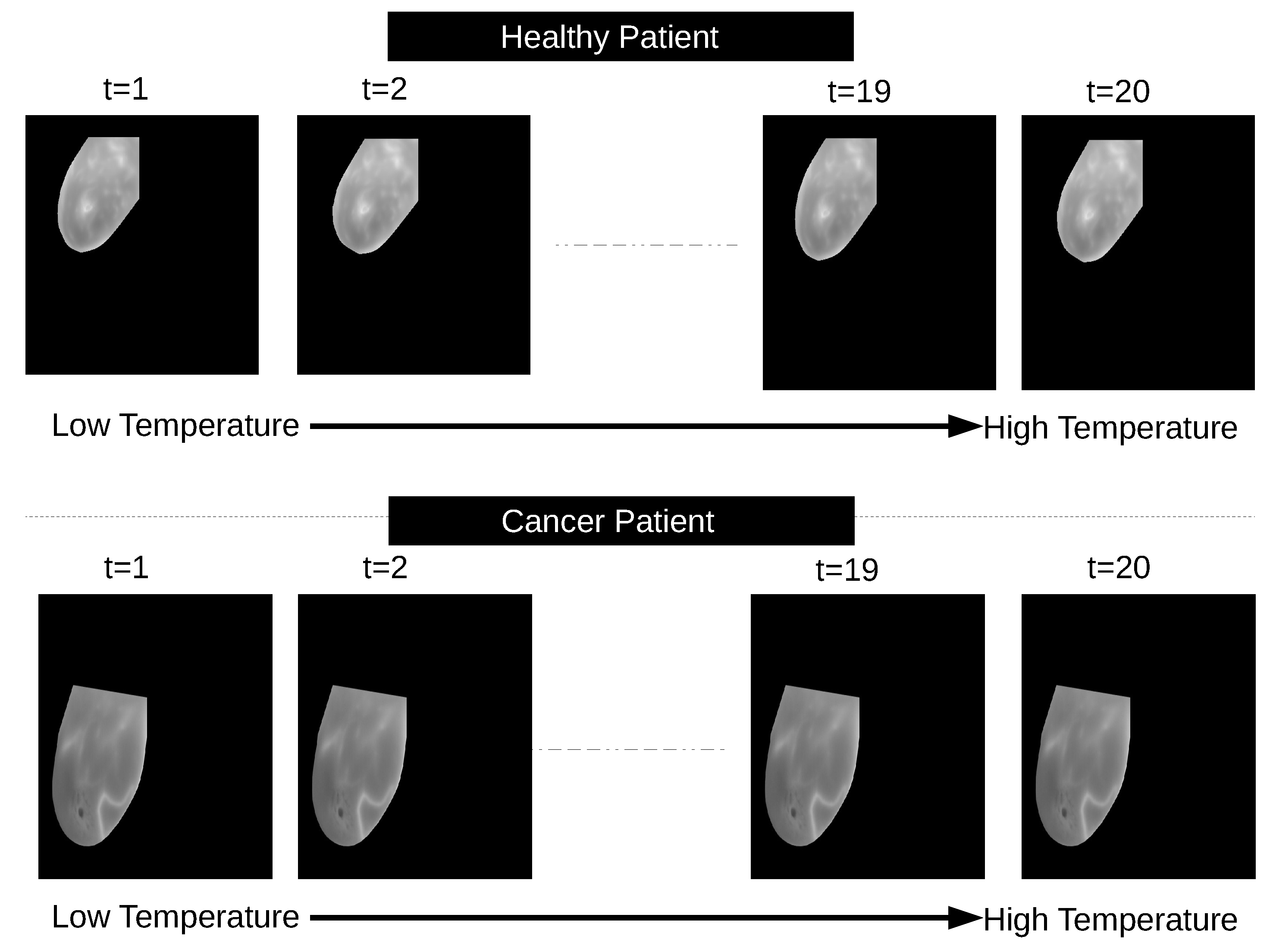
Dynamic infrared thermographies may enhance the detection results of static infrared images by employing a superficial stimulus to improve the thermal contrast [5]. Cooling or heating procedures can be exploited as a stimulus to thermally excite tissues of patients’ breasts. It is worth noting that the cooling procedure is much safer than the heating procedure as the temperature range of women body is C–C, and thus higher heating may harm the living tissues in the breasts. After applying the cooling procedure on the breasts, the temperature of healthy tissues decreases with an attenuation of vascular diameter; in turn, the temperature of abnormal tissues remains unaltered (or it increases with a vascular dilation), as reported in [6]. In this manner, the findings of the analysis of the similarity (or the dissimilarity) between infrared images acquired before and after the cooling procedure can be exploited to reveal breast cancer. Figure 1 shows samples of sequences of infrared images produced from a dynamic thermography procedure for a healthy case and a cancer patient. The dynamic thermography procedure generates a sequence of arrays for each patient. Each array is generated at a time step t and comprises the temperatures of the middle region of the patient’s body (specifically, the region between the neck and the waist). Examples of Figure 1 only show the temperature arrays of one breast for the two cases. Please note thatthe arrays that include the skin temperature (in Celsius) of the breasts are transformed into images.
In this paper, we propose a novel method for modeling the changes of temperature in the breasts during the dynamic thermography procedure using a representation learning technique called learning-to-rank (LTR) and texture analysis methods. We assess the performance of six texture analysis methods to describe the changes of breast temperatures in thermal infrared images: histogram of oriented gradients (HOG), features calculated from the gray level co-occurrence matrix (GLCM), lacunarity analysis of vascular networks (LVN), local binary pattern (LBP), local directional number pattern (LDN) and Gabor filters (GF). These texture analysis methods have been widely used in the literature to analyze breast cancer images. We use the LTR method to learn a representation for the whole sequence of infrared images. The LTR method produces a compact yet descriptive representation for each sequence of thermograms, which is then fed into a classifier to differentiate between healthy cases and cancer patients.
2. Related Work
Over the past two decades, several techniques have been presented for the early detection of breast cancer, such as mammography and MRI [7]. Sebastien et al. [8] presented a comparative study of several breast cancer detection techniques and discussed their main limitations. Hamidinekoo et al. [9] presented an overview of the recent state-of-the-art deep learning-based computer-aided diagnosis (CAD) systems developed for mammography and breast histopathology images. The authors proposed an approach to map features between mammographic abnormalities and the corresponding histopathological representations. Rampun et al. [10] proposed the use of local quinary patterns (LQP) for breast density classification in mammograms on various neighborhood topologies. Despite the fact that mammography is the standard method for early detection of breast cancer, its main drawback is that it may produce a large number of false positives [8]. In turn, the MRI technique is recommended as an adjunct to mammography for women with genetic mutations [11]. However, the main limitation of MRI is that it has a limited spatial resolution, yielding a low sensitivity for sub-centimeter lesions [12].
Infrared thermal imaging can overcome the limitations of the mammography technique because it can selectively optimize the contrast in areas of dense tissues (young women), as reported in [13]. Several methods have been proposed in the literature to analyze breast cancer using dynamic thermograms [14,15,16,17,18,19,20,21,22,23]. The authors of [24] reviewed different medical imaging modalities for computer-aided cancer detection methods with a focus on thermography. The authors of [25] presented a new method for extracting the region of interest (ROI) from breast thermograms by considering the lateral views and the frontal views of the breasts. The obtained ROIs help physicians to discriminate between the biomarkers of normal and abnormal cases. Mookiah et al. [26] evaluated the use of a discrete wavelet transform, texture descriptors, fuzzy and decision tree classifiers, to distinguish the normal cases from the abnormal ones. With 50 thermograms, their system achieved an average sensitivity of 86.70%, a specificity of 100% and an accuracy of 93.30%. Saniei et al. [27] proposed a five-step approach for analyzing the thermal images for cancer detection. The five steps are: (1) the breast region is extracted from the infrared images using the connected component labeling method, (2) the infrared images were aligned using a registration method, (3) the blood vessels were segmented using morphological operators, (4) for each vascular network, the branching points were exploited as thermal minutia points, and (5) the branching points were fed into a matching algorithm to classify breast regions into normal or abnormal, achieving a sensitivity of and a specificity of . Acharya et al. [28] extracted a co-occurrence matrix and a run length matrix texture features from each infrared image and then fed them into a support vector machine algorithm to discriminate the normal cases from the malignant ones, achieving a mean sensitivity of , a specificity of and an accuracy of . Furthermore, Etehadtavakol et al. [29] demonstrated the importance of extracting the hottest/coldest regions from thermographic images and used the Lazy snapping method (an interactive image cutout algorithm) to do so quickly with an easy detailed adjustment.
Gerasimova et al. [30] used the wavelet transform modulus maxima method in a multi-fractal analysis of time-series of breast temperatures obtained from dynamic thermograms. Homogeneous mono-fractal fluctuations statistics have been noticed from the temperature time-series obtained from breasts with malignant tumors. The authors of [31] used asymmetry features to classify breast thermograms while [32] used several feature extraction methods and hybrid classifiers to classify breast thermograms into normal or abnormal cases. In [33], statistical descriptors were extracted from thermograms and inputted into a fuzzy rule-based system to classify them into malignant or benign. The descriptors were collected from the two breasts of each case to quantify their bilateral changes. This method gave an accuracy of . Furthermore, the study of [34] proposed a three-step approach for identifying patients at risk of breast cancer. First, the infrared images of each case were registered. Second, the breast region was divided into kernels of pixels and the average temperature from each region was computed in all images of the same case. Then, two complexity features were computed from the thermal signals. Third, the k-means clustering method was used to construct two clusters from the feature vectors. Silhouette, Davies-Bouldin and Calinski-Harabasz indexes were computed and then used as descriptors. This method obtained an accuracy of using a decision tree classifier. In [35], a ground-truth-annotated breast thermogram database (DBT-TU-JU database) was proposed for the early prediction of breast lesions. The DBT-TU-JU database includes 1100 static thermograms of 100 cases.
Most of the methods proposed in the literature focus on the extraction of features from the images and do not consider the temporal evolution of temperature during the dynamic procedure (i.e., they ignore the temporal information in the infrared image sequences). Unlike the above-mentioned methods, we propose the use of the LTR method to generate a compact and robust representation of the whole sequence of infrared images of each case. The resulting representation models the evolution of temperature in the skin of breasts during the thermography procedure. Then, we use the generated representations to train a classifier to discriminate between healthy cases and cancer patients.
3. Proposed Method
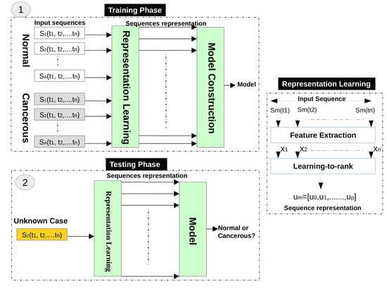
Figure 2 presents the proposed method for cancer detection in dynamic thermograms. It consists of two phases: training and testing. The training phase has two stages: representation learning and model construction. In the representation learning stage, we extract texture features from each thermogram, and then an LTR method is used to learn a compact and descriptive representation for the whole sequence. In the model construction stage, the learned representations are fed into a classifier to construct a model. This model is trained to discriminate between normal and cancerous cases. Please Please note thatthe representation learning step (feature extraction and LTR) does not use the ground truth of each sequence (i.e., the labels of each sequence: normal or cancer) to generate a compact representation of the infrared images of each sequence. The labels are only used to train a multilayer perceptron (MLP) classifier (the model construction stage of the training phase).
In the testing phase, we perform the first two steps of the training phase (feature extraction and LTR), and then we input the generated representations of test sequences into the model obtained in the training phase to predict their labels (normal/cancer). Below, we provide more details for each step of the proposed method.
3.1. Representation Learning
In this stage, we use six texture analysis methods to extract texture descriptors from each infrared image, and then the LTR method is exploited to generate a representation for the infrared images of each case.
3.1.1. Texture Analysis
To describe the texture of breast tissues in infrared images accurately, we assess the efficacy of six texture analysis methods: histogram of oriented gradients, lacunarity analysis of vascular networks, local binary pattern, local directional number pattern, Gabor filters and descriptors computed from the gray level co-occurrence matrix. These texture analysis methods have been widely used in medical image analysis and achieved good results with breast cancer image analysis [16,27,28,36,37,38].
Histogram of oriented gradients (HOG): The HOG method is considered as one of the most powerful texture analysis methods because it produces distinctive descriptors in the case of illumination changes and cluttered background [39]. The HOG method has been used in several studies to analyze medical images. For instance, in [16], a nipple detection algorithm was used to determine the ROIs and then the HOG method was used to detect breast cancer in infrared images. To construct the HOG descriptor, the occurrences of edge orientations in a local image neighborhood are accumulated. The input image is split into a set of blocks (each block includes small groups of cells). For each block, a weighted histogram is constructed, and then the frequencies in the histograms are normalized to compensate for the changes in illumination. Finally, the histograms of all blocks are concatenated to build the final HOG descriptor.
Lacunarity analysis of vascular networks (LVN): Lacunarity refers to a measure of how patterns clog the space [40] and describes spatial features, multi-fractal and even non-fractal patterns. We use the lacunarity of vascular networks (LVN) in thermograms to detect breast cancer. To calculate LVN features, we first extract the vascular network () from each infrared image and then calculate the lacunarity-related features . Please Please note thatLVN extracts 2 features from each infrared image. Below, we briefly explain the two stages:
- -
- Vascular network extraction: this method has two steps [27]:
- Step 1: Preprocess each infrared image using an anisotropic diffusion filter.
- Step 2: Use the black top-hat method to extract the VN from the preprocessed infrared images.
This process produces a binary image (i.e., VN is a binary image). In Figure 3, we show an example of a vascular network extracted from an infrared image. - -
- Lacunarity-related features: We use the sliding box method to determine the lacunarity on the binary image . In this method, an patch is moved through the image VN, and then we count the number of mass points within the patch at each position and compute a histogram ; n denotes the number of mass points in each patch. The histogram refers to the number of patches containing n mass points. The lacunarity at scale l for the pixel at the position can be determined as follows [40]:where calculates the expectation of the random variable X. The study of [41] demonstrated that the lacunarity shows power law behaviors with its scale l as follows:
We take the logarithm on left and right sides of Equation (2) to get the following equation:
To estimate and , we use the linear least squares fitting technique, and set the scale range to compute the lacunarity in the interval [42,43].
Gabor filters (GF): GF have been used in several works on medical image analysis. For instance, the authors of [44] extracted Gabor features from breast thermograms, such as energy and amplitude in different scales and orientations to quantify the asymmetry between normal and abnormal breast tissues. In [45], self-similar GF, the Karhunen–Loève (KL) transform and Otsu’s thresholding method were used to detect global signs of asymmetry in the fibro-glandular discs of the left and right mammograms of breast cancer patients. The KL transform was used to preserve the most relevant directional elements appearing at all scales. In [37], GF were used to extract directional features from mammographic images and the principal component analysis method was used for dimensionality reduction. In [46], GF were used to extract texture features from mammographic images to detect breast cancer.
The 2D Gabor filter can be formulated as a sinusoidal with a certain frequency and orientation multiplied by a Gaussian envelope as follows:
where , and are the standard deviations along the x- and y-axes, and the centre of the sinusoidal function, respectively. In our experiments, 4 scales and 6 orientations are used to compute GF responses (the number of scales and orientation were empirically tuned). Then, we convolve each input image with each response to determine the filtered image . To extract texture features from GF, the energy is computed from each filtered image, and then all energies are concatenated into one feature vector [47].
Local binary pattern (LBP): The LBP operator assigns a label (0 or 1) for each pixel in the input image. LBP extracts a box around each pixel and then compares all pixels with it. Pixels in this box with a value greater than are labelled by ‘1’ and the other pixels are labelled by ‘0’. In this way, LBP represents each pixel with 8-bits [36,48]. We only consider patterns that comprise at most two transitions from 1 to 0 or from 0 to 1 (called uniform LBPs). Please Please note that 10101010 is a non-uniform LBP and 00111110 is a uniform LBP. To construct the final LBP descriptor, we compute the histogram of uniform patterns (its length is 59).
Local directional number (LDN): Rámirez et al. proposed the LDN descriptor in [49], in which 8 Kirsch compass masks are convolved with the input image, yielding 8 edge responses for each pixel (each response is a result for a mask). The authors used a code for each mask (called location code): 000 for mask0, 001 for mask1, 010 for mask2, 011 for mask3, 100 for mask4, 101 for mask5, 110 for mask6 and 111 for mask7. For each pixel in the image, LDN determines the maximum positive and smallest negative edge responses, and then the location codes corresponding to the two responses are concatenated.
Assume that we convolve the eight masks (mask0–mask7) with an infrared image and we get eight edge responses (10, −20, 0, 3, 7, −10, 6, and 30) for the pixel . The maximum positive and smallest negative edge responses are 30 and −20 that correspond to the masks mask1 and mask7. Thus, the LDN code for the pixel is 111001. A 64-bin histogram is computed from the codes extracted from the input infrared images.
Features computed from the gray level co-occurrence matrix (GLCM): To compute the GLCM, we determine the joint frequencies of possible combinations of gray levels i and j in the input image. Please Please note thateach pair is separated by a distance and an angle [50]. In this research, we set the distance to 5 and use 4 different orientations (, , and ) with a quantification level of 32 to compute 22 descriptors from each GLCM. This configuration was recommended in several related studies, such as [38,51]. We then concatenate all descriptors into one feature vector (its dimension is 88, ). In Table 1, we present the descriptors extracted from the GLCM in addition to the mathematical expression of each descriptor [50,52,53]. The interpretation of terms used to compute the descriptors are provided in Table 2.
3.1.2. Representation Learning Using LTR
Based on the observation that the changes of temperatures on normal and abnormal tissues have a different temporal ordering, we use the LTR method to model the evolution of temperatures of women breasts during dynamic thermography procedures. In other words, we use the LTR method to generate a compact description for each image sequence. Assume that we have a sequence of thermograms of a breast (temperature matrices), and each thermogram at time t is represented by a vector , thus the whole sequence is represented by ; Nsq is the number of images in the sequence (in our case Nsq = 20). The feature vector of each thermogram is obtained in the feature extraction stage (Section 3.1.1).
We use the LTR method to model the relative rank of these thermograms (e.g., comes after , which can be written as ). Assume m3 is the feature vector of an infrared image acquired at time step t3, m2 is the feature vector of an infrared image acquired at time step t2, and m1 is the feature vector of an infrared image acquired at time step t1, this means that m3 comes after m2, and m2 comes after m1. We use the LTR method to model this ranking, which represents the change of temperature in breasts from a time step to another during the dynamic thermography procedure.
To avoid the effect of abrupt changes of temperatures in thermograms, the LTR method learns the order of smoothed versions of the feature vectors. Let us define a sequence , where is the result of processing the feature vectors from time 1 to t ( to ) using the time varying mean method as follows:
Each vector is then normalized as follows:
where is the normalized version of . Given the smoothed vectors, LTR learns their rank (i.e., ), a linear LTR learns a pairwise linear function , where is a vector containing its parameters. The ranking score of is computed by . The LTR method optimizes the parameters of using the objective function of Equation (7) with the constraint as follows [54]:
where is the regularization parameter and is the margin of tolerance. The constraint of the objective function encourages the ranking score (prediction score) of the difference between the feature vectors of two infrared images and acquired at time and , respectively, to be greater than , and the margin of tolerance should be greater than or equal zero. In other words, if comes after , the ranking score of should be greater than the one of . For further details the reader is referred to [55,56]. In our case, the temperature evolution information is encoded in the parameters , which can be viewed as a principled, data-driven, temporal pooling of the evolution of temperature in thermography procedures. Thus, the parameters are used in this study to describe the evolution of temperatures in the whole sequence of thermograms. In other words, we use to represent the whole sequence. In this study, we model the evolution of temperatures in thermography procedures in the forward and backward directions, as follows:
- Forward direction (): we model the changes in the temperature from the cooling instant to the instant of restoring the normal temperature of the body (the algorithm moves from the infrared image acquired at time step t to the image acquired at ).
- Backward direction (): we model the changes in temperature in the reverse direction where we start with the last infrared image of the input sequence and proceed to the first one (the algorithm moves from the infrared image acquired at time step t to the image acquired at ).
In our experiments, we calculate the parameters of LTR two times for each input sequence: one for the forward direction and another for the backward direction . Prior to the classification stage, we normalize each feature vector using the norm. In the classification stage, we input the feature vectors of normal and cancerous cases into the MLP classifier to construct a classification model.
3.2. Model Construction
We used the MLP classifer to classify the cases into normal or cancerous. MLP is a network of simple neurons called perceptrons. Each perceptron computes a single output from multiple numerical inputs by setting a weight for each input and then combining them. The combined value is then input into a non-linear activation function. Equation (8) formulates this operation as:
where is the output of the perceptron, x is the vector of inputs, is the vector of weights, is the bias and is the activation function. The common activation functions are the logistic sigmoid and the hyperbolic tangent . In this study, we use the latter one.
4. Evaluation Metrics and Statistical Analysis Methods
To evaluate the proposed method, we use five metrics: accuracy, recall, precision, F-score (the harmonic mean of the precision and recall) and the area under the curve (AUC) of the receiver operating characteristic (ROC) curve. True positive (TP), true negative (TN), false positive (FP) and false negative (FN) are determined to calculate the four metrics:
- TP refers to positive instances correctly classified as positive cases.
- TN refers to negative instances correctly classified as negative cases.
- FP refers to negative instances wrongly classified as positive cases.
- FN refers to positive instances wrongly classified as negative cases.
The mathematical expressions of accuracy, recall, precision and F-score are shown below:
The ROC analysis is used to avoid choosing a certain threshold for classifying the data [57]. We use each possible threshold to calculate the true positive rate and the false positive rate . In our experiments, we randomly split the dataset into training, validation, and testing sets. The training, validation and testing ratios were 0.7, 0.15 and 0.15. Please Please note thatall images/sequences pertaining to a given patient either all belong to the training set or the testing set (or validation set). The number of instances in each set is rounded to the nearest integer. To check if the model is overfitting or not, we randomly re-partition the DMR-IR dataset into training, validation and testing datasets. We repeat this process 100 times and report the mean value of AUC, accuracy, recall, precision and F-score.
To show the efficacy of the proposed method, we also calculate the statistical significance of the differences of results between our proposal and the other methods in terms of the AUC values. To do so, we use the Wilcoxon signed-rank test to find the difference in AUC values (significance level < 0.05). To check the normality of the distributions of the AUC values, we use the Shapiro-Wilk test. If we have comparisons and the significance level of a single experiment is 0.05, according to the Bonferroni correction the actual significance level should be [58]. Please note thata p-value lower than refers to statistically significant results.
5. Experimental Results and Discussion
5.1. Dataset
In our experiments, we use the dynamic thermogram dataset presented in [59] to validate our method. This database is called DMR-IR and it is available at http://visual.ic.uff.br/dmi/. The acquisition protocol of DMR-IR has the following steps:
- An electric fan was used for several minutes for cooling the breasts and armpits of patients (an environment with the temperature range C–C).
- A FLIR thermal camera was used to capture 20 infrared images during 5 min after the cooling (the dimension of the images is pixels).
The FLIR camera (model SC620) has a sensitivity smaller than C with a detectable temperature range between −C and C. DMR-IR has 37 sequences of cancer patients (histopathologically proven breast cancer) and 19 of healthy cases (without benign findings). It is worth mentioning that the DMR-IR dataset includes segmented images that contain only the temperatures of breasts (excluding the temperatures of other parts of the body). The medical records of each patient (age, race, personal history, family history, medical history and protocol recommendations) are given in the following website: http://visual.ic.uff.br/dmi/. It is worth mentioning that the DMR-IR dataset does not include information about breast density, breast size and lesion size.
5.2. Results
In our experiments, we only model the changes on temperatures in the breast region of thermograms. The dataset used includes masks for the breast regions (images containing the temperatures of breasts of each patient). To evaluate the proposed method, we carried out the following four experiments:
- Concatenation of the texture features extracted from each thermogram (without using the LTR method). In this way, we produce one feature vector for each sequence, which is then used to classify the cases.
- Use of the forward representation generated by the LTR method to classify the cases.
- Use of the backward representation generated by the LTR method to classify the cases.
- We concatenate the forward and backward representations of each sequence of thermograms, and then use it to classify the cases.
Table 3 presents the results of the texture analysis methods with the MLP classifier (50 neurons) when concatenating the feature vectors extracted from each thermogram (without using the LTR method). As shown, the HOG method with 4 blocks and 4 cells (HOG4*4) achieves an AUC value and an accuracy better than the ones of HOG2*2 (2 blocks, 2 cells), LVN, GF, LBP, LDN and GLCM. Please note that HOG4*4 has the highest dimension compared to the other texture analysis methods. Even though the LVN feature vector has the smallest dimension, it has better classification results than the GLCM. The main reason for the low performance of the GLCM is that it depends on the intensity of the pixels, making it more sensitive to the noise.
Table 4 presents the performance of the six texture analysis methods when using the representation learned by the forward LTR (i.e., ), finding that HOG2*2+ achieves the best AUC value, while LDN+ gives the best accuracy and score. Table 5 presents the results of each texture analysis method when using the representation learned by the backward LTR (i.e., ). In this case, HOG4*4+ achieves the best AUC value, accuracy, recall, precision and score. The results of the forward and the backward representations are better than the ones of the feature concatenation method. This is because of the temporal information encoded in the forward and the backward representations (i.e., the change from one infrared image to another over time). In turn, the feature concatenation method ignores such information.
In Table 6, we present the performance of the six texture analysis methods when concatenating the representations learned by the forward and backward LTR. HOG4*4+LTR (4 blocks, 4 cells, and with the concatenation of and ) gives classification results better than the ones of the other methods in terms of the five evaluation metrics. HOG2*2+LTR (4 blocks, 4 cells and with LTR) produces the second best classification results, but its dimensions are much lower than the ones of HOG4*4+LTR (72 with HOG2*2+LTR vs. 288 with HOG4*4+LTR). In general, the results of the HOG method with LTR are better than the ones of concatenating the features of all thermograms of each sequence, or the ones learned by or .
As summarized in Table 7, HOG, LVN, GF, LBP and LDN achieve the best AUC values when concatenating the representations learned by the forward and backward LTR. In turn, GLCM gives the best AUC value when using the representation learned by . The concatenation of the forward and backward representations provides a complete description of the evolution of the temperature in the breasts during the dynamic thermography (from the cooling instant to the warm instant and vice-versa). Thus, this concatenation yields accurate classification results. Unlike the feature concatenation approach, the time-varying mean used with the LTR method smooths the feature vector of each sequence, and thus it reduces the effect of abrupt changes of temperatures and suppresses the noise. There are two major reasons for the high performance of the HOG method with the LTR method (HOG4*4+):
- Unlike LBP, LDN and GLCM, HOG is less sensitive to the noise.
- In the HOG method, we accumulate the occurrence of the gradients of the temperature matrices along different orientations, and thus it produces an accurate description of the gradients of temperatures in the infrared images.
Indeed, the problem of having too many features describing an inductive learning task is the curse of dimensionality. In the case of GLCM, we calculate 22 descriptors, where each uses measures to extract a specific feature from the images (e.g., contrast and energy). When concatenating the forward and backward representations of GLCM, we get 176 features (88 × 2) that may make the model more expressive and maybe not all of these features are even relevant to our task. This explains why the results of the forward or the backward representation of the GLCM features (AUC values of 0.807 and 0.821) are better than the ones of concatenation (AUC = 0.677).
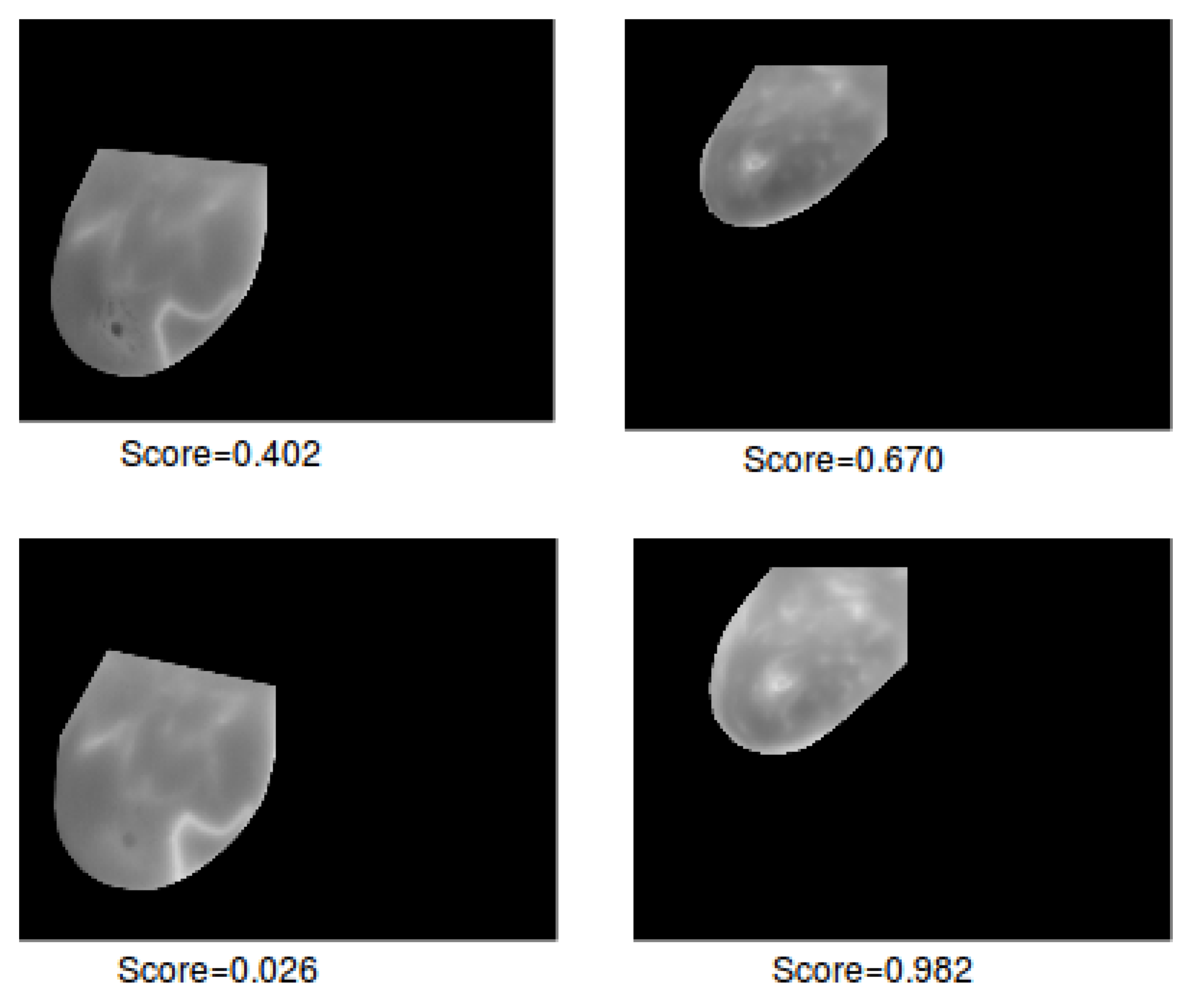
Malignancy score. The proposed method also assigns a degree of membership () for each case to be a malignant tumor (the malignancy score). The range of the malignancy score values is [0, 1]. If the malignancy score is close to 0, the probability of a malignant tumor decreases. In this paper, we exploit the likelihood score of the MLP classifier to compute the degree of membership for each case (the likelihood that a label comes from the malignant class). It is worth noting that the degree of membership of a given case to be healthy is . In Figure 4, we show the malignancy scores of our method (HOG4*4+) for two normal cases and two cancer patients. As we can see, the proposed method assigns small scores for normal cases ( < 0.5) and high scores for cancerous cases ( > 0.6).
Statistical analysis. The results of HOG4*4+LTR are better than those of individual texture analysis methods (Table 3). To show the efficacy of the proposed method, we also calculate the statistical significance of the differences of results between HOG4*4+LTR and the other methods in terms of the AUC values. The findings of the Shapiro-Wilk test showed that the AUC values do not follow a normal distribution. Given that we have 5 comparisons and the significance level of a single experiment is 0.05, according to the Bonferroni correction the actual significance level should be 0.01 (0.05/5). In Table 7, we present the statistical analysis of the AUC values. Table 7 shows that the AUC values of the HOG4*4+LTR are significantly better than the ones of the other combinations (Wilcoxon signed-rank test).
The experimental results demonstrate that the proposed method can model the changes on temperature across dynamic thermograms and produce a descriptive and compact representation of the whole sequence of infrared images, yielding good classification results between normal and cancer patients.
5.3. Comparison with the Related Work
In Table 8, we compare the proposed method with related studies. The authors of [27,34] used dynamic thermography databases, while [33] also used a static thermography database. As we can see in Table 8, the classification results with dynamic thermograms are much better than the ones with static thermograms. The authors of [34] (described in Section 2) also used the DMR-IR dataset in their study. In our experiments, we used all the samples of the DMR-IR dataset while [34] only used 22 samples, which are not enough to train, test and judge the efficacy of their method. In addition, they did not use any cross-validation method or statistical analysis method. In turn, to check if our model is overfitting or not, we randomly re-partitioned the DMR-IR dataset into training, validation and testing datasets and reported the average results. Our proposal (HOG4*4+LTR) gives an accuracy and precision better than the ones of [34]. In turn, we achieved an AUC value lower than the one of [34] because we used a larger number of samples to train and test our method.
Unlike the principal component thermography (PCT) [60] and the candid covariance-free incremental principal component thermography (CCIPCT) [61] that use matrix decomposition/ factorization to find the defects in thermal images and dimension reduction, in the proposed method we input the 20 infrared images of the breast for each subject (the whole sequence) into the LTR method to generate a compact representation for them. As shown in the results section, the LTR method yields classification results better than the ones of the concatenation of each texture analysis method.
6. Conclusions and Future Work
In this article, we have presented a new method for detecting breast cancer in dynamic thermograms. We model the changes in breast temperatures during the dynamic thermography procedures using the LTR and texture analysis methods. Our method generates a compact yet descriptive representation for the whole sequence of thermograms of each case. We then input the representation extracted from normal and cancerous cases into the MLP classifier to build a classification model. The proposed method obtains outstanding classification results in terms of AUC, accuracy, recall, precision and F-score. It also outperforms the results of related methods. To further improve the classification results, the future work will focus on using sparse dictionary learning to generate a more powerful description of infrared images.
Author Contributions
Conceptualization, M.A.-N., A.M. and D.P.; methodology, M.A.-N.; software, M.A.-N.; validation, M.A.-N., A.M. and D.P.; formal analysis, M.A.-N., A.M. and D.P.; investigation, M.A.-N.; resources, M.A.-N. and A.M.; data curation, M.A.-N.; writing—original draft preparation, M.A.-N.; writing—review and editing, A.M. and D.P.; visualization, M.A.-N.; supervision, A.M. and D.P.; project administration, D.P.; funding acquisition, D.P.
Funding
This research was partly supported by the Spanish Government through project DPI2016-77415-R.
Conflicts of Interest
The authors declare no conflict of interest.
Abbreviations
The following abbreviations are used in this manuscript:
| HOG | Histogram of oriented gradients |
| GLCM | Gray level co-occurrence matrix |
| LVN | Lacunarity analysis of vascular networks |
| VN | Vascular network |
| LBP | Local binary pattern |
| GF | Gabor filters |
| LDN | Local directional number pattern |
| LTR | Learning-to-rank |
| MLP | Multilayer perceptron |
| PM | Probability matrix |
| MPM | Marginal probability matrix |
| TP | True positive |
| TN | True negative |
| FP | False positive |
| FN | False negative |
| IM | Information measure |
| ID | Inverse difference |
References
- Malvezzi, M.; Carioli, G.; Bertuccio, P.; Boffetta, P.; Levi, F.; La Vecchia, C.; Negri, E. European cancer mortality predictions for the year 2018 with focus on colorectal cancer. Ann. Oncol. 2018, 29, 1016–1022. [Google Scholar] [CrossRef] [PubMed]
- Abdel-Nasser, M.; Moreno, A.; Puig, D. Temporal mammogram image registration using optimized curvilinear coordinates. Comput. Methods Progr. Biomed. 2016, 127, 1–14. [Google Scholar] [CrossRef] [PubMed]
- Chiarelli, A.M.; Prummel, M.V.; Muradali, D.; Shumak, R.S.; Majpruz, V.; Brown, P.; Jiang, H.; Done, S.J.; Yaffe, M.J. Digital versus screen-film mammography: impact of mammographic density and hormone therapy on breast cancer detection. Breast Cancer Res. Treat. 2015, 154, 377–387. [Google Scholar] [CrossRef] [PubMed]
- Faust, O.; Acharya, U.R.; Ng, E.Y.K.; Hong, T.J.; Yu, W. Application of infrared thermography in computer aided diagnosis. Infrared Phys. Technol. 2014, 66, 160–175. [Google Scholar] [CrossRef] [Green Version]
- Zhou, Y.; Herman, C. Optimization of skin cooling by computational modeling for early thermographic detection of breast cancer. Int. J. Heat Mass Transf. 2018, 126, 864–876. [Google Scholar] [CrossRef]
- Kennedy, D.A.; Lee, T.; Seely, D. A comparative review of thermography as a breast cancer screening technique. Integr. Cancer Ther. 2009, 8, 9–16. [Google Scholar] [CrossRef] [PubMed]
- Litjens, G.; Kooi, T.; Bejnordi, B.E.; Setio, A.A.A.; Ciompi, F.; Ghafoorian, M.; Van Der Laak, J.A.; Van Ginneken, B.; Sánchez, C.I. A survey on deep learning in medical image analysis. Med. Image Anal. 2017, 42, 60–88. [Google Scholar] [CrossRef] [Green Version]
- Mambou, S.; Maresova, P.; Krejcar, O.; Selamat, A.; Kuca, K. Breast Cancer Detection Using Infrared Thermal Imaging and a Deep Learning Model. Sensors 2018, 18, 2799. [Google Scholar] [CrossRef]
- Hamidinekoo, A.; Denton, E.; Rampun, A.; Honnor, K.; Zwiggelaar, R. Deep learning in mammography and breast histology, an overview and future trends. Med. Image Anal. 2018, 47, 45–67. [Google Scholar] [CrossRef]
- Rampun, A.; Scotney, B.W.; Morrow, P.J.; Wang, H.; Winder, J. Breast Density Classification Using Local Quinary Patterns with Various Neighbourhood Topologies. J. Imaging 2018, 4, 14. [Google Scholar] [CrossRef]
- Cho, N.; Han, W.; Han, B.K.; Bae, M.S.; Ko, E.S.; Nam, S.J.; Chae, E.Y.; Lee, J.W.; Kim, S.H.; Kang, B.J.; et al. Breast cancer screening with mammography plus ultrasonography or magnetic resonance imaging in women 50 years or younger at diagnosis and treated with breast conservation therapy. JAMA Oncol. 2017, 3, 1495–1502. [Google Scholar] [CrossRef] [PubMed]
- Boogerd, L.S.; Handgraaf, H.J.; Lam, H.D.; Huurman, V.A.; Farina-Sarasqueta, A.; Frangioni, J.V.; van de Velde, C.J.; Braat, A.E.; Vahrmeijer, A.L. Laparoscopic detection and resection of occult liver tumors of multiple cancer types using real-time near-infrared fluorescence guidance. Surg. Endosc. 2017, 31, 952–961. [Google Scholar] [CrossRef] [PubMed]
- Kosus, N.; Kosus, A.; Duran, M.; Simavlı, S.; Turhan, N. Comparison of standard mammography with digital mammography and digital infrared thermal imaging for breast cancer screening. J. Turk. German Gynecol. Assoc. 2010, 11, 152. [Google Scholar] [CrossRef] [PubMed]
- Díaz-Cortés, M.A.; Ortega-Sánchez, N.; Hinojosa, S.; Oliva, D.; Cuevas, E.; Rojas, R.; Demin, A. A multi-level thresholding method for breast thermograms analysis using Dragonfly algorithm. Infrared Phys. Technol. 2018, 93, 346–361. [Google Scholar] [CrossRef]
- Abdel-Nasser, M.; Saleh, A.; Moreno, A.; Puig, P. Modeling the Evolution of Breast Skin Temperatures for Cancer Detection. In Artificial Intelligence Research and Development: Proceedings of the 19th International Conference of the Catalan Association for Artificial Intelligence, Barcelona, Catalonia, Spain, 19–21 October 2016; IOS Press: Amsterdam, The Netherlands, 2016; p. 117. [Google Scholar]
- Abdel-Nasser, M.; Saleh, A.; Moreno, A.; Puig, D. Automatic nipple detection in breast thermograms. Expert Syst. Appl. 2016, 64, 365–374. [Google Scholar] [CrossRef]
- Boquete, L.; Ortega, S.; Miguel-Jiménez, J.M.; Rodríguez-Ascariz, J.M.; Blanco, R. Automated detection of breast cancer in thermal infrared images, based on independent component analysis. J. Med. Syst. 2012, 36, 103–111. [Google Scholar] [CrossRef] [PubMed]
- Marques, R.S. Segmentação Automática das Mamas em Imagens Térmicas. Master’s Thesis, Instituto de Computação, Universidade Federal Fluminense, Niterói, RJ, Brasil, 2012. [Google Scholar]
- Ng, E.K.; Fok, S.C.; Peh, Y.C.; Ng, F.C.; Sim, L.S.J. Computerized detection of breast cancer with artificial intelligence and thermograms. J. Med. Eng. Technol. 2002, 26, 152–157. [Google Scholar] [CrossRef]
- Qi, H.; Head, J.F. Asymmetry analysis using automatic segmentation and classification for breast cancer detection in thermograms. In Proceedings of the 23rd Annual International Conference of the IEEE Engineering in Medicine and Biology Society, Istanbul, Turkey, 25–28 October 2001; pp. 2866–2869. [Google Scholar]
- Krawczyk, B.; Schaefer, G.; Woźniak, M. A hybrid cost-sensitive ensemble for imbalanced breast thermogram classification. Artif. Intell. Med. 2015, 65, 219–227. [Google Scholar] [CrossRef]
- Chatfield, K.; Lempitsky, V.S.; Vedaldi, A.; Zisserman, A. The devil is in the details: an evaluation of recent feature encoding methods. In Proceedings of the 22nd British Machine Vision Conference (BMVC), University of Dundee, Dundee, UK, 29 August–2 September 2011; Volume 2, p. 8. [Google Scholar]
- Chanmugam, A.; Hatwar, R.; Herman, C. Thermal analysis of cancerous breast model. In Proceedings of the ASME International Mechanical Engineering Congress and Exposition, Houston, TX, USA, 9–15 November 2012; pp. 135–143. [Google Scholar]
- Sathish, D.; Kamath, S.; Rajagopal, K.V.; Prasad, K. Medical imaging techniques and computer aided diagnostic approaches for the detection of breast cancer with an emphasis on thermography—A review. Int. J. Med. Eng. Inform. 2016, 8, 275–299. [Google Scholar] [CrossRef]
- Josephine Selle, J.; Shenbagavalli, A.; Sriraam, N.; Venkatraman, B.; Jayashree, M.; Menaka, M. Automated recognition of ROIs for breast thermograms of lateral view—A pilot study. Quant. InfraRed Thermogr. J. 2018, 15, 194–213. [Google Scholar] [CrossRef]
- Mookiah, M.R.K.; Acharya, U.R.; Ng, E.Y.K. Data mining technique for breast cancer detection in thermograms using hybrid feature extraction strategy. Quant. InfraRed Thermogr. J. 2012, 9, 151–165. [Google Scholar] [CrossRef]
- Saniei, E.; Setayeshi, S.; Akbari, M.E.; Navid, M. A vascular network matching in dynamic thermography for breast cancer detection. Quant. InfraRed Thermogr. J. 2015, 12, 24–36. [Google Scholar] [CrossRef]
- Acharya, U.R.; Ng, E.Y.K.; Tan, J.H.; Sree, S.V. Thermography-based breast cancer detection using texture features and support vector machine. J. Med. Syst. 2012, 36, 1503–1510. [Google Scholar] [CrossRef] [PubMed]
- Etehadtavakol, M.; Emrani, Z.; Ng, E.Y.K. Rapid extraction of the hottest or coldest regions of medical thermographic images. Med. Biol. Eng. Comput. 2018, 1–10. [Google Scholar] [CrossRef] [PubMed]
- Gerasimova, E.; Audit, B.; Roux, S.G.; Khalil, A.; Argoul, F.; Naimark, O.; Arneodo, A. Multifractal analysis of dynamic infrared imaging of breast cancer. EPL (Europhys. Lett.) 2014, 104, 68001. [Google Scholar] [CrossRef]
- Nowak, R.M.; Okuniewski, R.; Oleszkiewicz, W.; Cichosz, P.; Jagodziński, D.; Matysiewicz, M.; Neumann, Ł. Asymmetry features for classification of thermograms in breast cancer detection. In Proceedings of the Photonics Applications in Astronomy, Communications, Industry, and High-Energy Physics Experiments, Wilga, Poland, 30 May–6 June 2016; p. 100312W. [Google Scholar]
- Gogoi, U.R.; Bhowmik, M.K.; Bhattacharjee, D.; Ghosh, A.K.; Majumdar, G. A study and analysis of hybrid intelligent techniques for breast cancer detection using breast thermograms. In Hybrid Soft Computing Approaches; Springer: New Delhi, India, 2016; pp. 329–359. [Google Scholar]
- Schaefer, G.; Závišek, M.; Nakashima, T. Thermography based breast cancer analysis using statistical features and fuzzy classification. Pattern Recognit. 2009, 42, 1133–1137. [Google Scholar] [CrossRef] [Green Version]
- Silva, L.F.; Sequeiros, G.O.; Santos, M.L.O.; Fontes, C.A.; Muchaluat-Saade, D.C.; Conci, A. Thermal Signal Analysis for Breast Cancer Risk Verification. In Proceedings of the World Congress on Medical and Health Informatics (MEDINFO2015), São Paulo, Brazil, 19–23 August 2015; pp. 746–750. [Google Scholar]
- Bhowmik, M.K.; Gogoi, U.R.; Majumdar, G.; Bhattacharjee, D.; Datta, D.; Ghosh, A.K. Designing of Ground-Truth-Annotated DBT-TU-JU Breast Thermogram Database Toward Early Abnormality Prediction. IEEE J. Biomed. Health Inform. 2018, 22, 1238–1249. [Google Scholar] [CrossRef]
- Abdel-Nasser, M.; Moreno, A.; Puig, D. Towards cost reduction of breast cancer diagnosis using mammography texture analysis. J. Exp. Theor. Artif. Intell. 2016, 28, 385–402. [Google Scholar] [CrossRef]
- Buciu, I.; Gacsadi, A. Directional features for automatic tumor classification of mammogram images. Biomed. Signal Process. Control 2011, 6, 370–378. [Google Scholar] [CrossRef]
- Gomez, W.; Pereira, W.C.A.; Infantosi, A.F.C. Analysis of co-occurrence texture statistics as a function of gray-level quantization for classifying breast ultrasound. IEEE Trans. Med. Imaging 2012, 31, 1889–1899. [Google Scholar] [CrossRef]
- Dalal, N.; Triggs, B. Histograms of oriented gradients for human detection. In Proceedings of the IEEE Computer Society Conference on Computer Vision and Pattern Recognition (CVPR’05), San Diego, CA, USA, 20–26 June 2005; pp. 886–893. [Google Scholar]
- Allain, C.; Cloitre, M. Characterizing the lacunarity of random and deterministic fractal sets. Phys. Rev. A 1991, 44, 3552. [Google Scholar] [CrossRef] [PubMed]
- Mandelbrot, B.B. The Fractal Geometry of Nature; WH Freeman: New York, NY, USA, 1982; Volume 1. [Google Scholar]
- Ali, M.A.; Sayed, G.I.; Gaber, T.; Hassanien, A.E.; Snasel, V.; Silva, L.F. Detection of breast abnormalities of thermograms based on a new segmentation method. In Proceedings of the Federated Conference on Computer Science and Information Systems (FedCSIS), Lodz, Poland, 13–16 September 2015; pp. 255–261. [Google Scholar]
- Borchartt, T.B.; Conci, A.; Lima, R.C.; Resmini, R.; Sanchez, A. Breast thermography from an image processing viewpoint: A survey. Signal Process. 2013, 93, 2785–2803. [Google Scholar] [CrossRef]
- Suganthi, S.S.; Ramakrishnan, S. Analysis of breast thermograms using gabor wavelet anisotropy index. J. Med. Syst. 2014, 38, 101. [Google Scholar] [CrossRef] [PubMed]
- Ferrari, R.J.; Rangayyan, R.M.; Desautels, J.L.; Frère, A.F. Analysis of asymmetry in mammograms via directional filtering with Gabor wavelets. IEEE Trans. Med. Imaging 2001, 20, 953–964. [Google Scholar] [CrossRef] [PubMed]
- Yousefi, B.; Ting, H.N.; Mirhassani, S.M.; Hosseini, M. Development of computer-aided detection of breast lesion using gabor-wavelet BASED features in mammographic images. In Proceedings of the IEEE International Conference on Control System, Computing and Engineering (ICCSCE), Penang, Malaysia, 29 November–1 December 2013; pp. 127–131. [Google Scholar]
- Weldon, T.P.; Higgins, W.E.; Dunn, D.F. Efficient Gabor filter design for texture segmentation. Pattern Recognit. 1996, 29, 2005–2015. [Google Scholar] [CrossRef] [Green Version]
- Ojala, T.; Pietikainen, M.; Maenpaa, T. Multiresolution gray-scale and rotation invariant texture classification with local binary patterns. IEEE Trans. Pattern Anal. Mach. Intell. 2002, 24, 971–987. [Google Scholar] [CrossRef] [Green Version]
- Rivera, A.R.; Castillo, J.R.; Chae, O.O. Local directional number pattern for face analysis: Face and expression recognition. IEEE Trans. Image Process. 2013, 22, 1740–1752. [Google Scholar] [CrossRef] [PubMed]
- Haralick, R.M.; Shanmugam, K. Textural features for image classification. IEEE Trans. Syst. Man Cybern. 1973, 6, 610–621. [Google Scholar] [CrossRef]
- Abdel-Nasser, M.; Melendez, J.; Moreno, A.; Omer, O.A.; Puig, D. Breast tumor classification in ultrasound images using texture analysis and super-resolution methods. Eng. Appl. Artif. Intell. 2017, 59, 84–92. [Google Scholar] [CrossRef]
- Soh, L.K.; Tsatsoulis, C. Texture analysis of SAR sea ice imagery using gray level co-occurrence matrices. IEEE Trans. Geosci. Remote Sens. 1999, 37, 780–795. [Google Scholar] [CrossRef] [Green Version]
- Clausi, D.A. An analysis of co-occurrence texture statistics as a function of grey level quantization. Can. J. Remote Sens. 2002, 28, 45–62. [Google Scholar] [CrossRef]
- Fernando, B.; Gavves, E.; Muselet, D.; Tuytelaars, T. Learning to rank based on subsequences. In Proceedings of the IEEE International Conference on Computer Vision (ICCV), Santiago, Chile, 13–16 December 2015; pp. 2785–2793. [Google Scholar]
- Joachims, T. Optimizing search engines using clickthrough data. In Proceedings of the 8th ACM SIGKDD International Conference on Knowledge Discovery and Data Mining, Edmonton, AB, Canada, 23–25 July 2002; pp. 133–142. [Google Scholar]
- Joachims, T. Training linear SVMs in linear time. In Proceedings of the 12th ACM SIGKDD International Conference on Knowledge Discovery and Data Mining, Philadelphia, PA, USA, 20–23 August 2006; pp. 217–226. [Google Scholar]
- Fawcett, T. An introduction to ROC analysis. Pattern Recognit. Lett. 2006, 27, 861–874. [Google Scholar] [CrossRef]
- Curtin, F.; Schulz, P. Multiple correlations and Bonferroni’s correction. Biol. Psychiatry 1998, 44, 775–777. [Google Scholar] [CrossRef]
- Silva, L.F.; Saade, D.C.M.; Sequeiros, G.O.; Silva, A.C.; Paiva, A.C.; Bravo, R.S.; Conci, A. A new database for breast research with infrared image. J. Med. Imaging Health Inform. 2014, 4, 92–100. [Google Scholar] [CrossRef]
- Rajic, N. Principal Component Thermography (No. DSTO-TR-1298); Defence Science and Technology Organisation Victoria (Australia) Aeronautical and Maritime Research Lab.: Melbourne, Australia, 2002. [Google Scholar]
- Yousefi, B.; Sfarra, S.; Castanedo, C.I.; Maldague, X.P. Comparative analysis on thermal non-destructive testing imagery applying Candid Covariance-Free Incremental Principal Component Thermography (CCIPCT). Infrared Phys. Technol. 2017, 85, 163–169. [Google Scholar] [CrossRef]
Sample Availability: The database used in this study is publicly available at http://visual.ic.uff.br/dmi/. |
Figure 1.
Samples of two dynamic thermogram sequences for two cases, where each sequence comprises 20 infrared images. The infrared images of the left breast acquired at different time steps () for a healthy case (top) and a cancer patient (bottom).
Figure 1.
Samples of two dynamic thermogram sequences for two cases, where each sequence comprises 20 infrared images. The infrared images of the left breast acquired at different time steps () for a healthy case (top) and a cancer patient (bottom).

Figure 2.
The training and testing phases of the proposed method.

Figure 3.
Lacunarity analysis of vascular networks extracted from infrared images, (a) the input infrared image, and (b) the extracted vascular network.
Figure 3.
Lacunarity analysis of vascular networks extracted from infrared images, (a) the input infrared image, and (b) the extracted vascular network.

Figure 4.
The malignancy score of two normal cases (left column) and two cancer patients (right column).
Figure 4.
The malignancy score of two normal cases (left column) and two cancer patients (right column).


Table 1.
Descriptors computed from the GLCM.
| Descriptor | Mathematical Expression |
|---|---|
| D01: Autocorrelation | |
| D02: Contrast | |
| D03: Correlation I | |
| D04: Correlation II | |
| D05: Cluster prominence | |
| D06: Cluster shade | |
| D07: Dissimilarity | |
| D08: Energy | |
| D09: Entropy | |
| D10: Homogeneity I | |
| D11: Homogeneity II | |
| D12: Maximum probability | |
| D13: Sum of squares | |
| D14: Sum average | |
| D15: Sum entropy | |
| D16: Sum variance | |
| D17: Difference variance | |
| D18: Difference entropy | |
| D19: Information measure (IM) of correlation I | |
| D20: IM of correlation II | |
| D21: Inverse difference (ID) normalized | |
| D22: ID moment normalized |
Table 2.
Interpretations for terms used to compute descriptors from the GLCM.
| Expression | Interpretation |
|---|---|
| The number of notable gray levels in the quantized image. | |
| GLCM size. | |
| The average of the entire normalized GLCM. | |
| entry in the marginal probability matrix (MPM) | |
| calculated by summing the rows of . | |
| entry in the MPM | |
| calculated by summing the columns of . | |
| and | Mean of and , respectively |
| and | Variance of and , respectively. |
| It accumulates the elements of probability matrix (PM) entries | |
| that correspond to the sum of a set of pairs of gray levels | |
| It accumulates the PM entries | |
| that correspond to the difference of a set of pairs of gray levels | |
| , and | Entropy of , and , respectively. |
| Term similar to the entropy equation used to calculate | |
| the IM of D19. | |
| Term similar to the entropy equation used to calculate | |
| the IM of D20. |
Table 3.
The performance of the proposed method when concatenating the feature vectors of the 20 infrared images of each sequence.
Table 3.
The performance of the proposed method when concatenating the feature vectors of the 20 infrared images of each sequence.
| Methods | Dimensions | AUC | Accuracy | Recall | Precision | F-Score |
|---|---|---|---|---|---|---|
| HOG2*2 | 720 | 0.946 | 0.913 | 0.937 | 0.902 | 0.919 |
| HOG4*4 | 2880 | 0.970 | 0.916 | 0.921 | 0.897 | 0.909 |
| LVN | 40 | 0.848 | 0.850 | 0.900 | 0.817 | 0.856 |
| GF | 960 | 0.856 | 0.871 | 0.844 | 0.914 | 0.874 |
| LBP | 1180 | 0.863 | 0.867 | 0.821 | 1.00 | 0.897 |
| LDN | 1280 | 0.935 | 0.914 | 1.00 | 0.829 | 0.895 |
| GLCM | 1760 | 0.673 | 0.633 | 0.613 | 0.821 | 0.691 |
Table 4.
The performance of the proposed method when using the representation learned by the forward LTR.
Table 4.
The performance of the proposed method when using the representation learned by the forward LTR.
| Methods | Dimensions | AUC | Accuracy | Recall | Precision | F-Score |
|---|---|---|---|---|---|---|
| HOG2*2+ | 36 | 0.972 | 0.911 | 0.930 | 0.894 | 0.902 |
| HOG4*4+ | 144 | 0.917 | 0.896 | 0.863 | 0.929 | 0.886 |
| LVN+ | 2 | 0.683 | 0.700 | 0.900 | 0.533 | 0.649 |
| GF+ | 48 | 0.935 | 0.879 | 0.885 | 0.858 | 0.860 |
| LBP+ | 59 | 0.945 | 0.919 | 0.982 | 0.865 | 0.911 |
| LDN+ | 64 | 0.918 | 0.920 | 0.947 | 0.902 | 0.913 |
| GLCM+ | 88 | 0.807 | 0.731 | 0.729 | 0.794 | 0.739 |
Table 5.
The performance of the proposed method when using the representation learned by the backward LTR.
Table 5.
The performance of the proposed method when using the representation learned by the backward LTR.
| Methods | Dimensions | AUC | Accuracy | Recall | Precision | F-Score |
|---|---|---|---|---|---|---|
| HOG2*2+ | 36 | 0.964 | 0.927 | 0.914 | 0.942 | 0.921 |
| HOG4*4+ | 144 | 0.983 | 0.961 | 0.962 | 0.963 | 0.959 |
| LVN+ | 2 | 0.708 | 0.700 | 0.583 | 0.750 | 0.650 |
| GF+ | 48 | 0.959 | 0.912 | 0.920 | 0.910 | 0.907 |
| LBP+ | 59 | 0.948 | 0.907 | 0.934 | 0.875 | 0.896 |
| LDN+ | 64 | 0.942 | 0.907 | 0.944 | 0.866 | 0.893 |
| GLCM+ | 88 | 0.821 | 0.719 | 0.742 | 0.688 | 0.684 |
Table 6.
The performance of the proposed method when concatenating the representations learned by the forward and backward LTR.
Table 6.
The performance of the proposed method when concatenating the representations learned by the forward and backward LTR.
| Methods | Dimensions | AUC | Accuracy | Recall | Precision | F-Score |
|---|---|---|---|---|---|---|
| HOG2*2+ | 72 | 0.983 | 0.951 | 0.971 | 0.926 | 0.943 |
| HOG4*4+ | 288 | 0.989 | 0.958 | 0.971 | 0.946 | 0.954 |
| LVN+ | 4 | 0.903 | 0.800 | 0.867 | 0.639 | 0.692 |
| GF+ | 96 | 0.973 | 0.925 | 0.975 | 0.879 | 0.917 |
| LBP+ | 118 | 0.987 | 0.912 | 1.00 | 0.827 | 0.895 |
| LDN+ | 128 | 0.945 | 0.896 | 0.963 | 0.818 | 0.871 |
| GLCM+ | 176 | 0.677 | 0.619 | 0.631 | 0.712 | 0.654 |
Table 7.
Statistical analysis.
| Methods | Best AUC Value | Configuration Led to the Best AUC Value | p-Value |
|---|---|---|---|
| HOG | 0.989 | HOG4*4+LTR | − |
| LVN | 0.903 | LVN+LTR | <0.001 |
| GF | 0.973 | GF+LTR | <0.001 |
| LBP | 0.987 | LBP+LTR | <0.001 |
| LDN | 0.945 | LDN+LTR | <0.001 |
| GLCM | 0.821 | GLCM+ | <0.001 |
Table 8.
Comparison with related studies.
| Methods | Features Used | Dataset | Dynamic | AUC | Accuracy | Recall | Precision | F-Score |
|---|---|---|---|---|---|---|---|---|
| HOG4*4+LTR | HOG features+LTR | All samples of DMR-IR database | yes | 0.989 | 0.958 | 0.971 | 0.946 | 0.954 |
| [34] | statistical features | 22 samples of DMR-IR database | yes | 1.00 | 0.901 | - | 0.93 | - |
| [27] | thermal minutia points | 50 thermograms of private dataset | yes | - | - | 0.86 | - | - |
| [33] | texture features | 146 thermograms of private dataset | no | - | 0.795 | 0.797 | - | - |
© 2019 by the authors. Licensee MDPI, Basel, Switzerland. This article is an open access article distributed under the terms and conditions of the Creative Commons Attribution (CC BY) license (http://creativecommons.org/licenses/by/4.0/).
Share and Cite
MDPI and ACS Style
Abdel-Nasser, M.; Moreno, A.; Puig, D. Breast Cancer Detection in Thermal Infrared Images Using Representation Learning and Texture Analysis Methods. Electronics 2019, 8, 100. https://doi.org/10.3390/electronics8010100
AMA Style
Abdel-Nasser M, Moreno A, Puig D. Breast Cancer Detection in Thermal Infrared Images Using Representation Learning and Texture Analysis Methods. Electronics. 2019; 8(1):100. https://doi.org/10.3390/electronics8010100
Chicago/Turabian StyleAbdel-Nasser, Mohamed, Antonio Moreno, and Domenec Puig. 2019. "Breast Cancer Detection in Thermal Infrared Images Using Representation Learning and Texture Analysis Methods" Electronics 8, no. 1: 100. https://doi.org/10.3390/electronics8010100
Note that from the first issue of 2016, this journal uses article numbers instead of page numbers. See further details here.