A High-Speed Division Algorithm for Modular Numbers Based on the Chinese Remainder Theorem with Fractions and Its Hardware Implementation

Abstract

In this paper, a new simplified iterative division algorithm for modular numbers that is optimized on the basis of the Chinese remainder theorem (CRT) with fractions is developed. It requires less computational resources than the CRT with integers and mixed radix number systems (MRNS). The main idea of the algorithm is (a) to transform the residual representation of the dividend and divisor into a weighted fixed-point code and (b) to find the higher power of 2 in the divisor written in a residue number system (RNS). This information is acquired using the CRT with fractions: higher power is defined by the number of zeros standing before the first significant digit. All intermediate calculations of the algorithm involve the operations of right shift and subtraction, which explains its good performance. Due to the abovementioned techniques, the algorithm has higher speed and consumes less computational resources, thereby being more appropriate for the multidigit division of modular numbers than the algorithms described earlier. The new algorithm suggested in this paper has O (log₂ Q) iterations, where Q is the quotient. For multidigit numbers, its modular division complexity is Q(N), where N denotes the number of bits in a certain fraction required to restore the number by remainders. Since the number N is written in a weighed system, the subtraction-based comparison runs very fast. Hence, this algorithm might be the best currently available.

1. Introduction

The development of an informational society poses new challenges connected with the problem of multidigit numbers transmission and processing. Important mathematical problems that require such calculations and also considerable computational resources, both in terms of theory and practice, arise in the applied and computational theory of numbers [1,2]. Most of such problems involve integer calculations with the numbers belonging to the large and super large computer ranges, while the results of calculations must be precise without rounding.

A feature of conventional computing devices is limited bit grid, which causes computational complexity for the operations over multidigit numbers.

For calculations with multidigit numbers or calculations with large-range numbers, the residue number systems (RNSs) have clear advantages over the radix number systems. Modern research is focused on the processing of multidigit data in which the values of integer variables considerably exceed the dynamic range of the serially produced computing devices (by 10³–10⁶ times and even more); see Molahosseini et al. [2].

Modular calculations are crucial for applications with multidigit numbers, e.g., cryptography, digital signature, and others [3,4].

For instance, the numbers used in cryptographic systems vary between $2^{600}$ and $2^{700}$ to guarantee the high-level security of protected information [5]. During modular processing these numbers are partitioned into small formats (several bits or several tens of bits), which appreciably speeds up their implementation.

Residue number systems attract many researchers as a base for computing devices, and the recent decade has been remarkable for the growing interest in these systems. This fact follows from numerous publications dedicated to RNS usage in digital signal processing, image processing, antinoise coding, cryptographic systems, quantum automata, neurocomputers, systems with the massive parallelism of operations, cloud computing, DNA computing, etc. [1,2,3,4,5,6,7,8,9,10,11,12,13].

Residue number systems are remarkable for fast summation, subtraction, and multiplication, which explains major interest in these systems for the applications requiring large volumes of calculations. However, some operations (modulo reduction, comparison and division of numbers) are very complicated in RNSs [14,15]. The development of more efficient algorithms for comparison, sign detection, and division would open up new applications of RNSs [16].

The existing division algorithms for RNSs [17,18,19] can be classified as the ones based on number comparison and the ones based on number subtraction.

In the comparison-based algorithms [18,19,20,21,22,23,24], the quotient is found using the iteration:

$$a^{\prime }=a-2^i{q}_{i}b$$

where $a^{\prime }$ and $a$ denote the current and next dividends, respectively; $b$ is the divisor; finally, $q_i$gives the digit of the quotient. For obtaining $q_i$, the quotient $a$ has to be compared with $2^{i}b$.

In the second class of the algorithms [21,25,26,27], the quotient is calculated using the iterations $a^{\prime }=a-Q_{i}b$. The quotient $Q_i$ is generated at each iteration from the complete RNS range, instead of being chosen from a small set.

The integer division algorithm [1] is similar to standard binary division. Yet, the main drawback of this algorithm and its modifications is that each iteration requires numbers comparison.

The algorithm without such drawbacks that was suggested in Szabó and Tanaka [1] replaces the real divisor with the approximate one (an RNS module or the product of several RNS moduli). The algorithm yields correct results under the condition $b\le \overline{b}<2b$, where $b$ and $\overline{b}$ are the real and approximate divisors, respectively. Clearly, this condition may be violated for some sets of moduli (e.g., $p_1=9,p_2=11,b=4$, where p₁ and p₂ are the RNS moduli).

Among the shortcomings of the above algorithm, note the need for using mixed radix number systems (MRNSs), scale operation, special logic and approximate divisor calculation tables. As a matter of fact, a series of approaches were proposed for solving the division problem based on the numbers comparison and sign detection methods, which can be classified in the following way: the algorithms [18,19,23] employ the conversions of MRNSs; the algorithms [18,22] formulate the problem in terms of even numbers detection (parity check); and the algorithms [20] involve the base extension method for iterations. However, the proposed algorithms suffer from high execution time and considerable hardware cost due to the usage of MRNS, the Chinese remainder theorem (CRT), and other time-consuming operations.

In Hiasat et al. [27] and Hiasat [24] it introduced a high-speed division algorithm in which the MRNS and CRT in modular numbers division were replaced by the comparison of the high powers of the dividend and divisor. The execution time and hardware cost of this algorithm are smaller in comparison with the other algorithms; nevertheless, it contains redundant stages. In order to speed up current quotient calculation, J.H. Yang [28] suggested a division algorithm based on parity check that finds the quotient twice as fast as the algorithms [24,27]. But the calculations of the high powers of 2 still require much time in RNSs, and these operations are performed at each iteration. In Chung [29] the original algorithm [27] was simplified using division by 2 and efficient quotient search within a probable range. At each round, this algorithm adopts hard-to-implement parity check, which is its disadvantage.

Most of the listed algorithms contain hard-to-implement operations such as the CRT, scale operation, extension, sign detection, and comparison, which reduce their speed and cause considerable hardware cost of modular numbers division.

There exists a division algorithm in the RNS format that uses the basic set of RNS moduli in combination with an auxiliary module system for storing the remainders of the dividend and divisor. The dividend and divisor in the RNS representation are converted into different RNS representations with different module systems [29]. The usage of two RNS sets leads to higher redundancy, making it necessary to perform direct and inverse transitions from the basic module set to the auxiliary one and back during division. This feature dramatically reduces the speed of calculations. Talahmeh at al. [30] introduced a fast division algorithm based on index transformations over the Galois field $GF\left(p\right)$, which is easily implemented using tabular search. However, this algorithm guarantees efficient processing for the data of 6–10 bits and prime moduli only. In the case of larger ranges, the algorithm has low performance because the generator of prime p must be very large to represent integers over the Galois field.

Most of the suggested iterative algorithms involve very many operations at each iteration. As was declared by the authors, the algorithm based on the CRT with fractions [22,26,31] might appear to be best because its time complexity is $O\left(nb\right)$, where $n$ denotes the number of RNS moduli and $b$ the number of bits in each module under the assumption that the moduli are more or less the same. But this algorithm has some disadvantages as follows: (a) the divisor D is limited by $\frac{P}{16}<D\le \frac{3P}{16}$, where P is an RNS representation range; (b) each iteration includes several operations such as summation, multiplication, comparison, and parity check; (c) in the end of the algorithm, the quotient has to be converted from the system $\left\{-1,0,1\right\}$ to the system $\left\{0,1\right\}$, which gives extra computation load during modular numbers division.

In this paper, an alternative modular division algorithm with efficient quotient calculation using the relative values of the dividend and divisor in the fractional representation is introduced. Each iteration of the new algorithm involves the shift and subtraction of the successive intermediate results, which makes hardware implementation more efficient.

2. Approximate Positional Characteristic Calculation for Modular Numbers Based on the CRT with Fractions and Its Application to Modular Division

An RNS is a set of positive and pairwise relatively prime numbers $\left\{p_1,p_2,\dots ,p_n\right\}$, which are called moduli or bases. The dynamic range is given by $P=p_1{p}_2\dots p_n$. For an unsigned number $х$, the additional RNS range has the form $0\le х\le Р-1$. For the signed numbers, the additional range is defined by $-\left[\frac{Р}{2}\right]<x\le \left[\frac{Р-1}{2}\right]$. In this system, any integer $а$ belonging to the range $\left[0,P-1\right]$ can be uniquely described by an ordered set of remainders $\left({\alpha }_1,{\alpha }_2,\dots ,{\alpha }_n\right)$. Each remainder ${\alpha }_i$ has the modulo $p_i$ representation

$${\alpha }_i=a\mathrm{mod}{p}_i={\left|a\right|}_{p_i},0\le {\alpha }_i<p_i,i=1,2,\dots ,n.$$

(1)

Let operation $\ast$ be arithmetic summation, subtraction or multiplication. The most interesting property of an RNS is that these operations can be converted from the integer representation into the modular operations with different moduli $p_i$, i.e.,

$$Z=а\ast b\stackrel{\mathrm{RNS}}{\to }\left\{\begin{array}{c}{\left|z\right|}_{p_1}={\left|{\alpha }_1\ast {\beta }_1\right|}_{p_1}\\ {\left|z\right|}_{p_2}={\left|{\alpha }_2\ast {\beta }_2\right|}_{p_2}\\ \dots \\ {\left|z\right|}_{p_n}={\left|{\alpha }_n\ast {\beta }_n\right|}_{p_n}\end{array}\right\}.$$

(2)

Using model Equation (2), the dynamic range is decomposed into parts with a narrower data format so that within them all calculations are performed in parallel. As a result, the complexity of the arithmetic structures decreases accordingly.

The number $а$ in the RNS representation can be restored using the Chinese Remainder Theorem [1,2], i.e.,

$$а={\left|{\displaystyle \sum _{i=1}^n\frac{P}{p_i}{\left|P_i^{-1}\right|}_{p_i}{\alpha }_i}\right|}_P,$$

(3)

where $P={\displaystyle \prod _{i=1}^n{p}_i}$; $p_i$, $i=1,2,\dots ,n$, denote the RNS moduli; ${\left|P_i^{-1}\right|}_{p_i}$ is the multiplicative inversion of $P_i$ on $p_i$, $P_i=\frac{P}{p_i}=p_1{p}_2\dots p_{i-1}{p}_{i+1}\dots p_n$.

As is well-known, among their drawbacks the RNSs have the implementation complexity of non-modular operations (comparison, division) that are based on given positional characteristics.

The analysis of positional characteristics shows that they can be calculated precisely or approximately. Therefore, the calculation methods of positional characteristics consist of two groups as follows:

• precise calculation methods;
• approximate calculation methods.

The precise calculation methods of positional characteristics were considered in [1,2]. In this paper, an approximate calculation method with appreciably smaller hardware cost and execution time for the operations over the positional codes of decreased digit capacity will be employed.

The approximate calculation method of positional characteristics uses the relative values of modular numbers with respect to the complete range defined by the Chinese Remainder Theorem [2]. This theorem associates with a positional number $a$ its remainder representation $\left({\alpha }_1,{\alpha }_2,\dots ,{\alpha }_n\right)$, where ${\alpha }_i$, $i=1,2,\dots ,n$, are the least non-negative residues of this number on the RNS moduli $p_1,p_2,\dots ,p_n$.

Assume that the number $а$ has the RNS representation with residues $\left\{{\alpha }_1,{\alpha }_2,\dots ,{\alpha }_n\right\}$. Dividing the left- and right-hand sides of Equation (3) by the constant $P$ (the dynamic range) yields the approximate value

$${\left|\frac{a}{P}\right|}_1={\left|{\displaystyle \sum _{i=1}^n\frac{{\left|P_i^{-1}\right|}_{p_i}}{p_i}{\alpha }_i}\right|}_1\approx {\left|{\displaystyle \sum _{i=1}^n{k}_i{\alpha }_i}\right|}_1.$$

(4)

Here $k_i=\frac{{\left|P_i^{-1}\right|}_{p_i}}{p_i}$ are the constants of the chosen system; ${\alpha }_i$, $i=1,2,\dots ,n$, denote the digits of the number in the RNS representation on the moduli $p_i$. Note that Equation (4) takes values within the interval $\left[0,1\right)$. The final value is obtained by summation and integer part truncation, with the fractional part being retained. The fractional value $F\left(a\right)={\left|\frac{a}{P}\right|}_1\in \left[0,1\right)$ contains information about the value of the number and its sign. If ${\left|\frac{a}{P}\right|}_1\in \left[0,\frac{1}{2}\right)$, then the number $a$ is positive, and $F\left(a\right)$ gives its value divided by $P$. Otherwise, $a$ is a negative number, and $1-F\left(a\right)$ gives its relative value. Denote by ${\left[F\left(a\right)\right]}_{2^{-t}}$ the value of $F\left(a\right)$ rounded to $2^{-t}$ bits. The exact value of $F\left(a\right)$ satisfies the inequalities ${\left[F\left(a\right)\right]}_{2^{-t}}<F\left(a\right)<{\left[F\left(a\right)\right]}_{2^{-t}}+2^{-t}$. The integer part of the number yielded by summing up $k_i$ is neglected, i.e., discarded.

The rounding of $F\left(a\right)$ causes inevitable errors. Introduce the notation $\rho =-n+{\displaystyle \sum _{i=1}^n{p}_i}$. As was demonstrated in [32], $N=\lceil {\log }_2\left(P\rho \right)\rceil$ bits after the decimal point have to be used for rounding $F\left(a\right)$ without considerable errors that would affect calculation accuracy. In other words, there exists a bijection between the set of numbers in the RNS representation and the set of numbers rounded to the $N$th bit, i.e., ${\left[F\left(a\right)\right]}_{2^{-N}}$.

Taking into account the function ${\left[F\left(a\right)\right]}_{2^{-N}}$, the sign detection conditions can be written as follows:

$$\begin{gathered} 1.\mathrm{If}а={\left[F\left(a\right)\right]}_{2^{-N}}<\frac{1}{2},\mathrm{then}\mathrm{the}\mathrm{number}a\mathrm{is}\mathrm{positive}. \\ 2.\mathrm{If}\frac{1}{2}\le {\left[F\left(a\right)\right]}_{2^{-N}}<1,\mathrm{then}\mathrm{the}\mathrm{number}a\mathrm{is}\mathrm{negative}. \end{gathered}$$

(5)

Consider the approximate calculation method for comparing numbers in the RNS representation.

Example. Let $p_1=2$, $p_2=3$, $p_3=5$, and $p_4=7$ be the system of RNS moduli. Then $P=2\cdot 3\cdot 5\cdot 7=210$, $\rho =2+3+5+7-4=13$, $P_1=\frac{P}{p_1}=105$, $P_2=\frac{P}{p_2}=70$, $P_3=\frac{P}{p_3}=42$, and $P_4=\frac{P}{p_4}=30$.

The constants $k_i$ for calculating the relative values are

$$k_1=\frac{{\left|\frac{1}{105}\right|}_2}{2}=\frac{1}{2},k_2=\frac{{\left|\frac{1}{70}\right|}_3}{3}=\frac{1}{3},k_3=\frac{{\left|\frac{1}{42}\right|}_5}{5}=\frac{3}{5},k_4=\frac{{\left|\frac{1}{30}\right|}_7}{7}=\frac{4}{7}$$

The constants $k_i$ rounded to 12 decimal places are

$$\begin{gathered} k_1=0.100000000000,k_2=0.010101010101, \\ {k}_3=0.100110011001,k_4=0.100100100100 \end{gathered}$$

Compare the two numbers $a=97$ and $b=96$ in the RNS representation with the moduli $p_1$, $p_2$, $p_3$, and $p_4$. Note that, for numbers comparison, the critical case is the numbers differing by 1. The RNS representations of the numbers $a$ and $b$ are $a=\left(1,1,2,6\right)$ and $b=\left(0,0,1,5\right)$, respectively. Their difference is $a-b=\left(1,1,2,6\right)-\left(0,0,1,5\right)=\left(1,1,1,1\right)$. Now, detect the sign of $a-b$. First, find ${\left[F\left(a-b\right)\right]}_{2^{-12}}=0.000000010010$; this value satisfies the first condition of model Equation (5), i.e., $0<0.000000010010<0.1$. Hence, the natural conclusion is that $a-b>0$, meaning $a>b$.

3. New Division Algorithm Based on the CRT with Fractions

Consider two numbers––a dividend $a=\left({\alpha }_1,{\alpha }_2,\dots ,{\alpha }_n\right)$ and a divisor $b=\left({\beta }_1,{\beta }_2,\dots ,{\beta }_n\right)$. Let both numbers be represented within the range $\left[0,P\right)$, where $P=p_1\cdot p_2\cdot \dots \cdot p_n$ and $p_i$, $i=1,2,\dots ,n$, denote the RNS moduli. For the sake of simplicity, assume that $a$ and $b$ are positive numbers. (The case of negative numbers can be considered by analogy using simple modifications.) The division algorithm calculates the quotient $Q$ and the remainder $R$ so that $a=Q\cdot b+R$, where $0\le R<b$. The detailed description of this algorithm is given in Appendix A.

Modular division includes two stages. At the first stage, the high power of $2^j$ is obtained using the binary series approximation of the quotient; at the second stage, the approximation series is refined accordingly. The algorithm yields $Q=\left(Q_1,Q_2,\dots ,Q_n\right)$, where $Q_i={\left|{\displaystyle \sum _{j\in L}{q}_j{2}^j}\right|}_{p_i}$; $L$ denotes the set of powers $j$ in the refined quotient approximation series; $p_i$, $i=1,2,\dots ,n$, are the RNS moduli.

For modular division optimization, the classical CRT will be replaced by the CRT with fractions. In this case, following model Equation (4), the dividend, divisor, and remainder can be written as the fractions

$$F(a)={\left|\frac{a}{P}\right|}_1,F(b)={\left|\frac{b}{P}\right|}_1,F(R)={\left|\frac{R}{P}\right|}_1.$$

Using the approximate values, consider the modular division algorithm based on the CRT with fractions.

The algorithm consists of two stages. The first stage is to find the high power $j$ of the divisor by the left shift of $F(b)$ to the zero digits standing before the first significant digit. At the second stage, the general quotient is generated by selecting the powers of 2 that form the partial quotients to be included in the general quotient approximation series. The analysis procedure starts from the highest power $j$ and ends with the zeroth power of 2, thereby reading out the necessary powers of 2 in the RNS representation. The modular division algorithm based on the CRT with fractions works in the following way. The residues table for the $0\left({\log }_{2}P-1\right)$ integer powers of 2 is put into memory, and the representations $a=\left({\alpha }_1,{\alpha }_2,\dots ,{\alpha }_n\right)$ and $b=\left({\beta }_1,{\beta }_2,\dots ,{\beta }_n\right)$, $\left({\alpha }_i,{\beta }_i\right)\mathrm{mod}{p}_i,i=1,2,\dots ,n$, are obtained at the input. Then the quotient is calculated so that $F(a)=\left(Q\mathrm{mod}{p}_1,Q\mathrm{mod}{p}_2,\dots ,Q\mathrm{mod}{p}_n\right)F(R)+F(b)$, where $0\le F(R)<F(b)$.

The quotient $Q=\lfloor \frac{a}{b}\rfloor$ is generated at each iteration from the powers of 2 in the RNS representation that are included or excluded depending on the sign of the subtraction chain ${\Delta }_i-{\Delta }_{i-1}-{\Delta }_{i-2}-\dots -{\Delta }_m$, ${\Delta }_i={\Delta }_{i-1}-2^{j-i}{q}_{j-i}F\left(b\right)$. The notations in this formula are the following: $j$ as the highest power of the quotient; $q_j$ as the highest digit of the quotient; $i$ as current iteration; ${\Delta }_1=F\left(a\right)-F\left(b\right)q_j{2}^j\approx {\left[F\left(a\right)\right]}_{2^{-t}}-\left[F\left(b\right)\right]{}_{2^{-t}}{q}_j{2}^j$; $1\le i,j<\lfloor {\log }_{2}P\rfloor$; $F\left(a\right)={\left|\frac{a}{P}\right|}_1$ and $F\left(b\right)={\left|\frac{b}{P}\right|}_1$ as the fractions; $P={\displaystyle \prod _{i=1}^n{p}_i}$ as the complete range; $p_i$, $i=1,2,\dots ,n$, as the RNS moduli; ${\left[F\left(a,b\right)\right]}_{2^{-t}}<F\left(a,b\right)<{\left[F\left(a,b\right)\right]}_{2^{-t}}+2^{-t}$; ${\left[F\left(a\right)\right]}_{2^{-t}}$ and ${\left[F\left(b\right)\right]}_{2^{-t}}$ as the values of $F\left(a\right)$ and $F\left(b\right)$, respectively, rounded to the $2^{-t}$th bit (note that the resulting errors do not affect calculation accuracy); ${\Delta }_i$ as the current value and ${\Delta }_{i-1}$ as the successive value, which is defined by the one-position right shift of the divisor multiplied by the corresponding power of 2 (actually, this is equivalent to division by 2 and the subtraction ${\Delta }_i-{\Delta }_{i-1}$). Each $i$th iteration is associated with the $i$th binary digit in the RNS representation, which are put into memory as the residuals table for the integer powers of 2.

The well-known algorithm needs the dividend and divisor at each iteration. For the new algorithm, the dividend $F(a)$ and the divisor $F(b)$ are required only at the first iteration; all subsequent iterations involve the difference ${\Delta }_i-{\Delta }_{i-1}$ because these values contain information about the dividend and divisor. With this method, all quotient approximation iterations are reduced to the subtraction ${\Delta }_i-{\Delta }_{i-1}$, and the sign of this difference is used to find the desired partial quotient as the corresponding power of 2 in the RNS representation. As a result, the computational complexity of modular division considerably decreases.

The digits of the quotient are obtained by the $\mathrm{mod}{p}_i$ summation of the partial quotients using the sign of the subtraction result. If the sign is positive, the quotient is included (otherwise excluded). In contrast to the well-known algorithms, the new one allows for easy implementation: the time complexity of the iterations is defined by the execution time of shift, subtraction, and summation.

Concerning the advantages of the new algorithm, note that the division procedure does not involve (a) intermediate numeric data in the MRNS representation and (b) difficult-to-implement RNS operations such as comparison, scaling, base extension, and sign detection. These features contribute to higher efficiency of modular division.

The new modular division algorithm for integer numbers $\left[\frac{a}{b}\right]$ has the scheme presented in Appendix B. The hardware implementation of this algorithm is described in detail below.

4. Hardware Implementation of New Modular Division Algorithm

The new modular division algorithm for multidigit numbers includes the following basic parts: quotient sign detection, quotient approximation, and further refinement of the quotient approximation series.

Figure 1 illustrates the hardware implementation of the modular division algorithm, which consists of several units such as converters, summers (summators), multipliers and others. The issues of their optimization were studied in the papers [33,34,35,36].

Assume that an RNS contains $n$ moduli and $n$ modular processors. Let $m$ be the number of bits required for the representation of each remainder. For making the hardware implementation complexity analysis of this algorithm simpler, consider the case in which the moduli are more or less the same. Under this hypothesis, the total length of the modular processor bus is $M=n\cdot m$ bits.

Let the dividend and divisor be arbitrary integers and also let the divisor be not reducible to a pairwise relatively prime number on the RNS moduli.

The hardware implementation scheme in Figure 1 includes buses $a$ and $b$ supplying the dividend and divisor, respectively, and quotient bus $Q$. Each of buses $a,b$, and $Q$ has $M$ bits. For division, the one-bit signal is supplied through «Division» bus. Upon receipt of the inputs $a$ and $b$, the system calculates $Q$ so that $a=Q\cdot b+R$, where $0\le R<b$.

At the initial state, the control unit (CU) receives the “Division” signal and then forms the following signals through the one-bit buses (see Figure 1):

• “Adj. 0,” for adjusting the zero states of the functional units;
• timing pulses («TP»), for performing control of the registers and counters;
• “Adj. MS,” for adjusting the address code of multiplexer («MS») 2:1;
• “Adj. DMS,” for adjusting the address code of demultiplexer («DMS») 1:2. Depending on the address code, demultiplexer «DMS»switches the highest power of 2, either simultaneously to multiplier «MTP» and element «OR» or to element «OR» only, whose output is connected to the input of inhibit element $I_1$. Depending on the address code, multiplexer MS switches to the output of the comparison and sign detection unit (CSDU), or directly to the divisor $b$, or to the divisor $b$ multiplied by the highest power of $2^k$;
• “Adj. $R{G}_1$,” for adjusting the right shift of reversible register $R{G}_1$;
• “Adj. CSDU,” for adjusting the blocking of the comparison and sign detection unit (CSDU).

The dividend $a$ and the divisor $b$ in the RNS representation on the chosen moduli are supplied through the M-bit buses to the input of CSDU. And this unit calculates the relative values of the dividend and divisor (${\left[F\left(a\right)\right]}_{2^{-N}}$ and ${\left[F\left(b\right)\right]}_{2^{-N}}$) as well as detects their signs and performs their comparison. Through element $I_3$ the dividend directly comes to the input of CSDU. And the divisor is supplied to the input of CSDU through multiplexer MS, which has the corresponding address at the address input. The CSDU is implemented by Equations (4) and (5) and the model of Example 1. If ${\left[F\left(a\right)\right]}_{2^{-N}}={\left|\frac{a}{P}\right|}_1<{\left[F\left(b\right)\right]}_{2^{-N}}={\left|\frac{b}{P}\right|}_1$, then CSDU forms the signal $b>a$ (the divisor is greater than the dividend), which comes to the input of the control unit. Next, the division unit is adjusted to the initial state, and the quotient $Q=0$. If ${\left[F\left(a\right)\right]}_{2^{-N}}={\left|\frac{a}{P}\right|}_1={\left[F\left(b\right)\right]}_{2^{-N}}={\left|\frac{b}{P}\right|}_1$, then CSDU generates the equality signal of the dividend and divisor (“$a=b$”). This signal is supplied to the input of summer $S{M}_3$, where the constant $1={\left(1,1,1,1\right)}_{RNS}$ is written. If ${\left[F\left(a\right)\right]}_{2^{-N}}={\left|\frac{a}{P}\right|}_1>{\left[F\left(b\right)\right]}_{2^{-N}}={\left|\frac{b}{P}\right|}_1$, then CSDU forms the signal “$a>b$,” and the control unit switches the division unit into the partial quotient approximation mode.

Next, the signs of the dividend $a$ and divisor $b$ are analyzed. The sign of the quotient $Q$ is defined by $signQ=signa\oplus signb=signa\overline{signb}+\overline{signa}signb$. From the output of CSDU the sign signals of the dividend and divisor (“$signa$” and “$signb$”) are supplied through the one-bit buses to the input of element exclusive or «XOR» (addition modulo 2). Using the truth table, this circuit generates the signal “$a=0$” or “$a=1$,” which is supplied to the input of quotient summer $S{M}_3$. If the output signal of element XOR is 0, then the quotient is assigned the positive sign (0); if it is 1, then the quotient is assigned the negative sign (1). Then, through the N-bit buses the values ${\left[F\left(a\right)\right]}_{2^{-N}}$ and ${\left[F\left(b\right)\right]}_{2^{-N}}$ come to the input of summer $S{M}_1$ and the shift register $R{G}_1$, respectively.

The value $F\left(a\right)$ is converted by $S{M}_1$ into the additional code, and the result is supplied to the input of subtractor $S{M}_2$ through the N-bit bus. The value ${\left[F\left(b\right)\right]}_{2^{-N}}$ comes to the input of reversible shift register $R{G}_1$ through the N-bit bus. Using the timing pulses of the control unit, the content of register $R{G}_1$ (the value ${\left[F\left(b\right)\right]}_{2^{-N}}$) is shifted to the right to the number of zero digits standing before the first significant digit; this number is registered by counter 2 «CNT2». The resulting number of shifts corresponds to the highest power $j$ of 2 in the divisor. The relative values are used to find the highest power of 2 in the quotient approximation series, which is registered by counter CNT2 without iterative calculations. As soon as the high significant digit of the divisor ${\left[F\left(b\right)\right]}_{2^{-N}}$ becomes 1 during the shift procedure (similar to number normalization), register $R{G}_1$ fixes the state of counter CNT2 through the one-bit bus and enables information read-out from $RAM$ (similarly to stack pointer). Counter CNT2 activates the RAM memory address defining the highest power of $2^j$ in the quotient approximation series that must be in the quotient $Q=\left[\frac{a}{b}\right]$. In the initial state, buffer register $R{G}_2$ has zero value. The quotient approximation mode is completed, and at the $RAM$ output the memory cell is activated that stores the highest power of $2^j$ in the quotient approximation series. Thus, for approximating the quotient $b$, the CSDU performs one comparison and one operation $\left[\log n\right]$ for obtaining the sum of N-bit numbers, while register $R{G}_1$ performs one shift operation to $j$ digits.

Let ${\left[F\left(b\right)\right]}_{2^{-t}}=0.000010100001$; in this case, after shifting the content of register $R{G}_1$ the state of counter CNT2 is $0011$. This counter activates the memory cell containing the power of $2^3\stackrel{RNS}{\to }\left({\left|2^3\right|}_{p_1},{\left|2^3\right|}_{p_2},\dots ,{\left|2^3\right|}_{p_n}\right)$.

4.1. Refinement Mode for Quotient Approximation Series with Dividend a and Divisor b

Recall that the highest power of $2^j$ is obtained in the approximation mode and stored by $RAM$ in the RNS representation. Using the one-bit signal “Adj. DMS,” this power comes through the M-bit memory bus to the input of summer $S{M}_3$ via elements OR and $I_1$. After that, through the one-bit bus “Adj. MS” the address code of multiplexer MS is adjusted to the next state; the value $b{2}^j$ is switched at the output of multiplexer MS and then supplied to the input of CSDU through the M-bit bus. This unit calculates ${\left[F\left(b{2}^j\right)\right]}_{2^{-N}}$ and sends the result to the input of shift register $R{G}_1$ through the N-bit bus $F\left(b\right)$. The old information in $R{G}_1$ is removed. The buses of the dividend а and divisor $b$ are disconnected from CSDU by the signal “Adj. CSDU” coming to the inputs of $I_3$ and $I_4$. Using the control signals of the control unit, the content of $R{G}_1$ is supplied to an input of $S{M}_2$ through the N-bit bus. From the output of summer $S{M}_1$ the value $F\left(a\right)$ is supplied to the second input of summer $S{M}_2$ through the N-bit bus. Next, the signal “Adj. $R{G}_1$” switches register $R{G}_1$ into the right shift mode.

The divisor multiplied by the highest power of 2 is subtracted from the content of summer $S{M}_2$, and the value ${\left[F\left(a\right)\right]}_{2^{-N}}-{\left[F\left(b{2}^k\right)\right]}_{2^{-N}}$ is calculated for detecting the sign of the result. If the sign digit of the subtraction result in summer $S{M}_2$ is 0, i.e., ${\left[F\left(a\right)\right]}_{2^{-N}}>{\left[F\left(b{2}^k\right)\right]}_{2^{-N}}$, then 0s are supplied to the inhibit inputs of inhibit elements $I_1$ and $I_2$. Through elements OR the inhibit elements $I_1$ and $I_2$ pass the highest power of the quotient from the second output of DMS to the input of summer $S{M}_3$. The subtraction result in summer $S{M}_2$ (i.e., the remainder of the dividend that corresponds to the rest powers of 2) is supplied, through the N-bit bus and inhibit element $I_2$, first to the input of buffer register $R{G}_2$ and then to the input of summer $S{M}_1$. The old content of this summer is removed, and the new value is written. Next, the content of register $R{G}_1$ is shifted to the right, and the process is repeated as described above. If the sign digit of the subtraction result in summer $S{M}_2$ is 1 (i.e., the relative value of the divisor is greater than the dividend), then this 1 comes to the inhibit inputs of elements $I_1$ and $I_2$ that inhibit the supply of the corresponding power to summer $S{M}_3$ and also the supply of the subtraction result of summer $S{M}_2$ to the input of buffer register $R{G}_2$. In other words, the register saves the previous value of the subtraction result. At its input summer $S{M}_3$ receives only the refined powers of 2 that are the terms of the quotient series. The conversion process ends after analyzing the power of $2^0$. Thus, in the refinement mode all redundant terms of the quotient approximation series are iteratively eliminated using uncomplicated transformations.

The approximate quotient is sequentially refined by the subtraction of the divisor first multiplied by the highest power of 2 from the dividend and its further shift and subtraction from the resulting partial remainders during quotient calculation. In comparison with the well-known algorithms, a distinctive feature of the quotient approximation refinement procedure suggested in the new algorithm is the usage of the dividend $а$ and the product $b{2}^j$ (the divisor and the highest power of 2) only at the first iteration. The subsequent iterations are based on an original principle of this paper, namely, on the one-position right shift of $b{2}^j$ at each iteration; in fact, this is equivalent to division by 2 and the subtraction of the results obtained at successive iterations, i.e., ${\Delta }_j-{\Delta }_{j-1}$. The principle is unique because each iteration contains two operations––one-position right shift and subtraction with further sign detection. As a result, the speed of division considerably increases. Each iteration of the well-known algorithms involves multiplication, summation, comparison, and parity check. Assume that each iteration requires $t$ time units; then the total time of each iteration is $4t$. Each iteration of the new algorithm consists of one subtraction and one shift, consuming $2t$ time units. Thus, the efficiency gain is about 2. The performance analysis of the new algorithm (quotient approximation and refinement) has demonstrated its considerable advantage over the well-known counterparts in terms of modular division time.

4.2. Experimental Performance Analysis: New Modular Division Algorithm Versus Well-Known Algorithms

As is indicated by experiments, the algorithm developed in this paper strongly depends on initial data (the number of RNS moduli and their values) and also on input data (the values of dividend and divisors). Hence, this algorithm is difficult for analytical study.

The new modular division algorithm is similar to the algorithm presented in Hung [25]. However, in comparison with the optimization methods used therein, the operations of multiplication and summation have been replaced by the less demanding shift operations of partial quotients based on comparison. As a result, hardware cost and execution time have been considerably reduced. Besides, the Lu–Chiang algorithm involves the quotient correction operator with sign detection using MRNS, which dramatically decreases its speed.

In this section, the algorithm [25] will be compared with the new modular division algorithm on the same numerical data. For comparison, choose the example considered in Hung [25].

Let the RNS moduli be 5, 7, 9, and 11.

For example, take the dividend $a=125=\left(0,6,8,4\right)$ and the divisor $b=14=\left(4,0,5,3\right)$. It is required to obtain the quotient $a=8=\left(3,1,8,8\right)$ and the remainder $r=13=\left(3,6,4,2\right)$.

For the sake of illustrative and complete analysis,

Table 1. Calculation of $\frac{125}{14}$ by algorithm [25].

Iteration	Variable	Value	RNS Moduli {5,7,9,11}	Notes
$\begin{array}{l}j=0\\ \\ \\ j=1\\ \\ j=2\\ \\ j=3\\ \\ j=4\\ \\ j=5\\ \end{array}$	$\begin{array}{l}D\\ \left[P/8\right]\\ \left[P/8\right]-2D\\ D=2D\\ \left[P/8\right]-2D\\ D=2D\\ \left[P/8\right]-2D\\ D=2D\\ \left[P/8\right]-2D\\ D=2D\\ \left[P/8\right]-2D\\ D=2D\\ \left[P/8\right]-2D\end{array}$	$\begin{array}{l}14\\ 433\\ 405\\ 28\\ 377\\ 56\\ 321\\ 112\\ 209\\ 224\\ -15\\ 448\\ -463\end{array}$	$\begin{array}{l}(4,0,5,3)\\ (3,6,1,4)\\ (0,6,0,9)\\ (3,0,1,6)\\ (2,6,8,3)\\ (1,0,2,1)\\ (1,6,6,2)\\ (2,0,4,2)\\ (4,6,2,0)\\ (4,0,8,4)\\ (0,6,3,7)\\ (3,0,7,8)\\ (2,6,5,10)\end{array}$	$\begin{array}{l}P=3465\\ \\ E{F}_{\alpha }=6/64,E{S}_{\alpha }=+\\ \\ E{F}_{\alpha }=5/64,E{S}_{\alpha }=+\\ \\ E{F}_{\alpha }=4/64,E{S}_{\alpha }=+\\ \\ E{F}_{\alpha }=2/64,E{S}_{\alpha }=+\\ \\ E{F}_{\alpha }=62/64,E{S}_{\alpha }=\pm \\ \\ E{F}_{\alpha }=54/64,E{S}_{\alpha }=-\end{array}$
Line 3	$\begin{array}{l}A\\ A-D\end{array}$	$\begin{array}{l}125\\ -323\end{array}$	$\begin{array}{l}(0,6,8,4)\\ (2,6,1,7)\end{array}$	$\begin{array}{l}\\ E{F}_{\alpha }=56/64,E{S}_{\alpha }=-\end{array}$
$\begin{array}{l}i=1\\ \\ \\ i=2\\ \\ i=3\\ \\ i=4\\ \\ i=5\\ \end{array}$	$\begin{array}{l}A\\ A=2(A-D)\\ Q=2(Q+1)\\ A=2(A+D)\\ Q=2(Q-1)\\ A=2(A+D)\\ Q=2(Q-1)\\ A=2(A-D)\\ Q=2(Q+1)\\ A=2(A+D)\\ Q=2(Q-1)\end{array}$	$\begin{array}{l}125\\ -646\\ 2\\ -396\\ 2\\ 104\\ 2\\ -688\\ 6\\ -480\\ 10\end{array}$	$\begin{array}{l}(0,6,8,4)\\ (4,5,2,3)\\ (2,2,2,2)\\ (4,3,0,0)\\ (2,2,2,2)\\ (4,6,5,5)\\ (2,2,2,2)\\ (2,5,5,5)\\ (1,6,6,6)\\ (0,3,6,4)\\ (0,3,1,10)\end{array}$	$\begin{array}{l}E{F}_{\alpha }=1/64,E{S}_{\alpha }=+\\ E{F}_{\alpha }=50/64,E{S}_{\alpha }=-\\ \\ E{F}_{\alpha }=56/64,E{S}_{\alpha }=-\\ \\ E{F}_{\alpha }=0/64,E{S}_{\alpha }=+\\ \\ E{F}_{\alpha }=50/64,E{S}_{\alpha }=-\\ \\ E{F}_{\alpha }=54/64,E{S}_{\alpha }=-\end{array}$
$\begin{array}{l}Line11\\ \\ Line15\\ \\ Line16\end{array}$	$\begin{array}{l}A=A+D\\ Q=Q-1\\ A=A+D\\ Q=Q-1\\ 2^j\\ 2^{-j}\\ R=2^{-j}A\end{array}$	$\begin{array}{l}32\\ 9\\ 416\\ 8\\ 32\\ 758\\ 13\end{array}$	$\begin{array}{l}(3,3,4,1)\\ (4,2,0,9)\\ (1,3,2,9)\\ (3,1,8,8)\\ (2,4,5,10)\\ (3,2,2,10)\\ (3,6,4,2)\end{array}$	$\begin{array}{l}E{F}_{\alpha }=61/64,E{S}_{\alpha }=\pm ,S=-\\ \\ \\ Quotient=8\\ \\ \\ \\ Remainder=13\end{array}$

and

Table 2. Calculation of $\frac{125}{14}$ by new algorithm.

Iteration	Variable	Value	RNS Moduli {5,7,9,11}	Notes
Line 1	a	125	(0,6,8,4)	P = 3465
	F_a = F(b)	1,210,464 × 2−25	-	-
	b	14	(4,0,5,3)	-
	F_b = F(b)	135,565 × 2−25	-	F_a − F_b = 1074899 × 2−25, “+”
j = 0	F_b = 2F_b	271,130 × 2−25	-	F_a – F_b = 939,334 × 2−25, “+”
j = 1	F_b = 2F_b	542,260 × 2−25	-	F_a – F_b = 668,204 × 2−25, “+”
j = 2	F_b = 2F_b	1,084,520 × 2−25	-	F_a – F_b = 125,944 × 2−25, “+”
j =3	F_b = 2F_b	2,169,040 × 2−25	-	F_a – F_b = –958,576 × 2−25, “–”
Line 6	F_b = F_b/2	1,084,520 × 2−25	-	-
Line 7	Δ1 = F_a – F_b	125,944 × 2−25	-	-
Line 8	Q = 2j	8	(3,1,8,8)	-
j = 2	F_b = F_b/2	1,084,520 × 2−25	-	Δ1 – F_b = –958,576 × 2−25, “–”
-	Q	8	(3,1,8,8)	-
j = 1	F_b = F_b/2	542,260 × 2−25	-	Δ1 – F_b = –416316 × 2−25, “–”
-	Q	8	(3,1,8,8)	-
j = 0	F_b = F_b/2	271,130 × 2−25	-	Δ1 – F_b = –145,186 × 2−25, “–”
-	Q	Quotient = 8	Quotient = (3,1,8,8)	-
Line 14	R = a – b·Q	Remainder = 13

provide intermediate data yielded by the algorithm [25] and the new algorithm, respectively, in the course of calculating $\frac{a}{b}=\frac{125}{14}$.

The new modular division algorithm is attractive owing to less operations (see

Table 3. Comparison of Hung-Parhami algorithms with new algorithm.

Operations	First Hung–Parhami Algorithm	Second Hung–Parhami Algorithm	New Algorithm
Operations in radix number system (summation, subtraction, multiplication)	54	71	18
Modular operations in RNS (modular summation, subtraction, multiplication)	45	53	5
Bit shift operations (left shift, right shift)	6	16	8
Nonmodular operations in RNS (sign detection)	1	1	0

). Table 3 shows how many operations of different types are consumed by the well-known algorithms and the new algorithm for the example [25] (these data were obtained by experimental study).

While using the new modular division algorithm, the division specifics of fractions must be considered for avoiding rounding errors.

Actually, the function ${\left[F\left(a\right)\right]}_{2^{-N}}$ is an approximate variation of the function $F\left(a\right)$. When RNS numbers are replaced by their approximate characteristics, an important issue is the accuracy of the representation ${\left[F\left(a\right)\right]}_{2^{-N}}$ that guarantees correct results of the division operation. In accordance with the experimental studies [30,32,37], the values of $N$ that are used for rounding and also for restoring the positional representation of numbers can be insufficient in several cases. This aspect may considerably restrict the performance of the device.

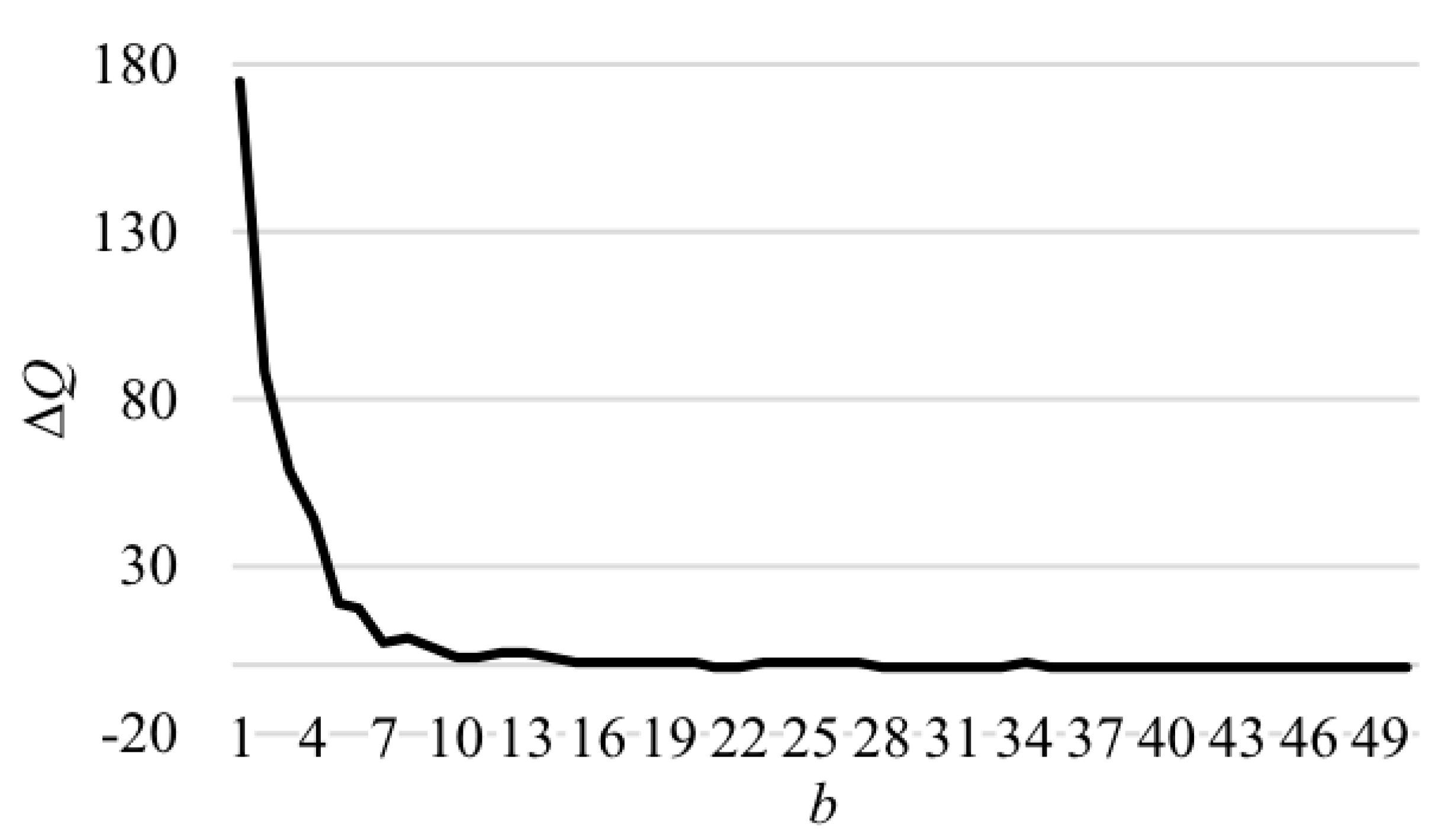
Consider the error of the division operation. For given numbers $a$ and $b$ in the RNS representation, the exact quotient $Q=a/b$ is approximated by the partial quotient

$$Q*=\frac{{\left[F\left(a\right)\right]}_{2^{-N}}}{{\left[F\left(b\right)\right]}_{2^{-N}}}.$$

In the quotient calculation problem, the algorithm outputs the integer part of the number $Q*$, which corresponds to the integer part of the exact quotient $Q$. The absolute error of the quotient is bounded by

$$\Delta Q*\le \frac{{\left[F\left(a\right)\right]}_{2^{-N}}\cdot \Delta F\left(a\right)+{\left[F\left(b\right)\right]}_{2^{-N}}\cdot \Delta F\left(b\right)}{{\left({\left[F\left(b\right)\right]}_{2^{-N}}\right)}^2},$$

(6)

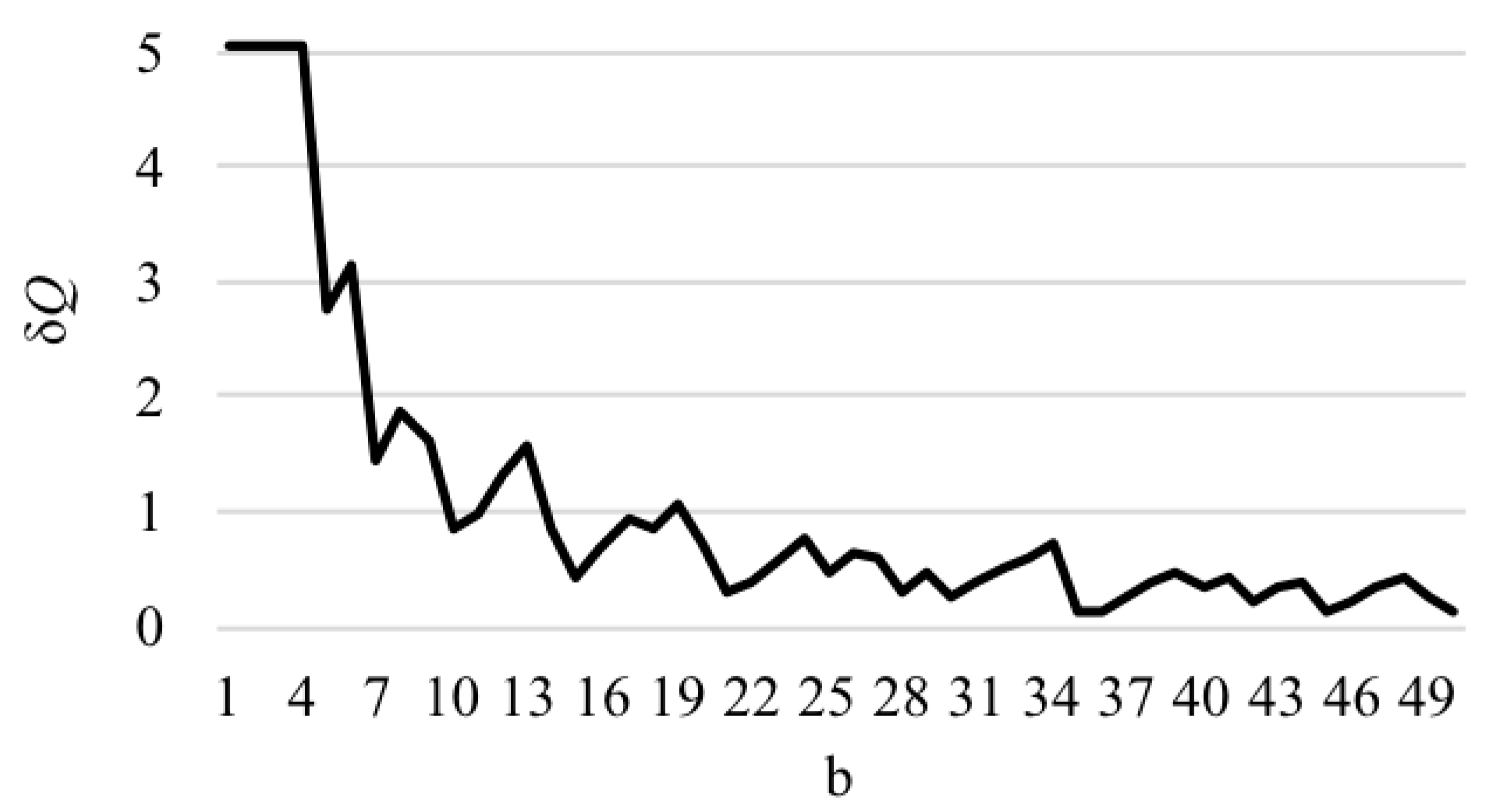
where $\Delta F\left(a\right)$ and $\Delta F\left(b\right)$ denote the calculation errors of the functions ${\left[F\left(a\right)\right]}_{2^{-N}}$ and ${\left[F\left(b\right)\right]}_{2^{-N}}$, respectively. Clearly, the absolute error of the quotient is growing as the dividend increases. However, special role is played by the divisor. In the current problem, the inequality ${\left[F\left(a\right)\right]}_{2^{-N}}<1$ always holds; hence, the denominator of the right-hand side of Equation (6) decreases faster than the numerator, and the error is rapidly growing for sufficiently small b (see the graph in Figure 2). The relative error is demonstrated in Figure 3.

Using Equation (6), estimate the value of $N$ that guarantees exact division. Note that the function $F\left(a\right)$ can be calculated by the equation

$$F\left(a\right)=\frac{a}{P}={\left|{\displaystyle \sum _{i=1}^n{k}_i{\alpha }_i}\right|}_1={\displaystyle \sum _{i=1}^n{k}_i{\alpha }_i}-r_a,$$

where $r_a$ gives the rank of number $a$. By analogy with this formula, the rounded value of the function ${\left[F\left(a\right)\right]}_{2^{-N}}$ is obtained using the constants $k_i^{*}$ rounded to $N$ decimal points, i.e.,

$${\left[F\left(a\right)\right]}_{2^{-N}}={\left|{\displaystyle \sum _{i=1}^n{k}_i^{*}{\alpha }_i}\right|}_1={\displaystyle \sum _{i=1}^n{k}_i^{*}{\alpha }_i}-r_a.$$

For each $k_i^{*}$, the inequality $\Delta k_i^{*}\le 2^{-N}$ holds. This yields the following estimate for the calculation error of ${\left[F\left(a\right)\right]}_{2^{-N}}$:

$$\Delta F\left(a\right)\le 2^{-N}{\displaystyle \sum _{i=1}^n{\alpha }_i}\le 2^{-N}\rho ,$$

where $\rho =p_1+p_2+\dots +p_n-n$.

Furthermore, the value ${\left[F\left(a\right)\right]}_{2^{-N}}$ converges to the exact value $F\left(a\right)$ as $N$ is increased. If the constants $k_i$ are rounded down, then the relationship

$${\left[F\left(a\right)\right]}_{2^{-N}}\le F\left(a\right)$$

holds for all $a$ from the RNS range.

Taking this inequality into account, Equation (1) can be rewritten as

$$\begin{gathered} \Delta Q*\le \frac{{\left[F\left(a\right)\right]}_{2^{-N}}\cdot \Delta F\left(a\right)+{\left[F\left(b\right)\right]}_{2^{-N}}\cdot \Delta F\left(b\right)}{{\left({\left[F\left(b\right)\right]}_{2^{-N}}\right)}^2}\le 2^{-N}\rho \frac{F\left(a\right)+F\left(b\right)}{{\left({\left[F\left(b\right)\right]}_{2^{-N}}\right)}^2}\approx \\ \approx 2^{-N}\rho \frac{F\left(a\right)+F\left(b\right)}{{\left(F\left(b\right)\right)}^2}=2^{-n}\rho P\frac{a+b}{b^2}. \end{gathered}$$

(7)

In view of the earlier notes, consider the worst case causing the largest error of calculations. Choose $a=P-1$ as the largest possible dividend and $a=1$ as the smallest possible divisor. Using Equation (7),

$$\Delta Q*\le 2^{-N}\rho P\frac{P-1+1}{1}=2^{-N}\rho P^2$$

Now, require that the error $\Delta Q*$ does not exceed a given threshold $\epsilon <1$. Then

$$\Delta Q*\le 2^{-N}\rho P^2\le \epsilon .$$

Solving this inequality in $N$ yields

$$N\ge {\log }_2\frac{\rho P^2}{\epsilon }$$

The integer parts of the approximate and exact quotients coincide if $\epsilon =0.005$. Using experimental studies, it was established that the threshold $\epsilon =0.5$ is sufficient for exact calculations. As a result, the final bound takes the form

$$N\ge {\log }_{2}2\rho P^2$$

(8)

The right-hand side of Equation (8) is greater than the lower bound in the inequality

$$N\ge {\log }_2\rho P$$

(9)

which is required for the exact number restoration in the algorithm.

Table 4. Distribution of division errors with insufficient rounding accuracy of $N$ for different sets of RNS moduli.

Set of RNS Moduli	Number of Digits for Exact Restoration N, Bits (Equation (9))	Range of Inadmissible Divisors	Share of Faulty Divisions, %	Number of Digits for Exact Division N, Bits (Equation (8))	Amount of Wrong Divisions, %
2, 3, 5, 7	12	1–14	6.67	19	0
2, 3, 5, 7, 11	16	1–154	6.71	26	0
5, 7, 9, 11	17	1–165	4.76	27	0
2, 3, 5, 7, 11, 13	21	1–858	2.86	34	0
2, 3, 5, 7, 11, 13, 17	25	1–31,907	6.25	42	0
2, 3, 5, 7, 11, 13, 17, 19	30	1–510,510	5.26	51	0
2, 3, 5, 7, 11, 13, 17, 19, 23	35	1–8,262,699	3.70	60	0
Moduli 2n − 1, 2n, 2n + 1, 22n+1 − 1
n = 2	17	1–81	4.41	25	0
n = 3	24	1–5819	9.09	35	0
n = 4	31	1–297,840	14.29	45	0
n = 5	38	1–779,193	1.16	55	0
Moduli 2n − 1, 2n + 1, 22n, 22n + 1
n = 2	18	1–80	1.99	27	0
n = 3	26	1–3360	1.28	39	0
n = 4	34	1–82,240	0.49	51	0
n = 5	42	1–4,364,800	0.41	63	0

shows the distribution of modular division errors with this bound for different RNS moduli. In addition to the general-form moduli, some sets of special form are also considered. Note that the share of faulty divisions varies from 0.5% to 14.3%. In accordance with Table 4, bound Equation (8) can be applied for exact division in RNS without any restrictions. Note that this approach and division in RNSs are difficult for theoretical study.

In their paper, Hung and Parhami [25] imposed a strict constraint on the choice of the divisor: it was recommended to use any divisors from the range $\frac{P}{16}<b<\frac{3P}{16}$, which considerably restricts the method’s applicability. The new approach suggested in this paper adopts bound Equation (8) for the number of digits without any constraints on the divisor.

On the other hand, the algorithms [25] and the new algorithm are comparable in terms of hardware cost and execution time for the MRNS operations (summation, subtraction, multiplication) and bit shift operations (right and left shifts). Really, the new algorithm requires less operations of these types, but the operands have higher digit capacity.

5. Conclusions

The new algorithm described in this paper speeds up the modular division procedure in the RNS representation in comparison with the well-known counterparts. This fact can be explained by the rather simple structure of the algorithm containing uncomplicated operations, namely, summation and shift (for quotient approximation) as well as shift and subtraction (for quotient refinement). Being based on the CRT with fractions, the new algorithm does not include such operations as modular remainder calculation and number conversion into the MRNS representation. In comparison with the well-known RNS division algorithms, the new modular division algorithm has several considerable advantages. First, the division procedure involves no additional constraints on the dividend and divisor, such as representation range constraints. The only requirement of the new algorithm is that both parameters belong to the RNS range. Second, the new algorithm does not include any non-modular operation. Furthermore, the new algorithm uses less modular operations (modular summation, subtraction, multiplication) than some other RNS division algorithms. The new algorithm considerably differs from the abovementioned ones. It is unique in the sense that iterations contain shifts and subtractions. In comparison with the existing analogs, this algorithm appreciably decreases hardware cost and execution time for modular division.

The developed division algorithm can be used to design arithmetic-logic RNS devices and also to design problem-oriented RNS processors for digital signal processing, cryptography, etc. These new RNS applications will promote further development of this field of computational mathematics.