An FPGA-Based CNN Accelerator Integrating Depthwise Separable Convolution


School of Electronics and Information Engineering, Harbin Institute of Technology, Harbin 150001, China
*
Author to whom correspondence should be addressed.
Electronics 2019, 8(3), 281; https://doi.org/10.3390/electronics8030281
Submission received: 29 December 2018
/
Revised: 8 February 2019
/
Accepted: 23 February 2019
/
Published: 3 March 2019
(This article belongs to the Special Issue Convolutional Neural Network Design and Hardware Implementation for Real-Time Vision Applications)
Abstract
:The Convolutional Neural Network (CNN) has been used in many fields and has achieved remarkable results, such as image classification, face detection, and speech recognition. Compared to GPU (graphics processing unit) and ASIC, a FPGA (field programmable gate array)-based CNN accelerator has great advantages due to its low power consumption and reconfigurable property. However, FPGA’s extremely limited resources and CNN’s huge amount of parameters and computational complexity pose great challenges to the design. Based on the ZYNQ heterogeneous platform and the coordination of resource and bandwidth issues with the roofline model, the CNN accelerator we designed can accelerate both standard convolution and depthwise separable convolution with a high hardware resource rate. The accelerator can handle network layers of different scales through parameter configuration and maximizes bandwidth and achieves full pipelined by using a data stream interface and ping-pong on-chip cache. The experimental results show that the accelerator designed in this paper can achieve 17.11GOPS for 32bit floating point when it can also accelerate depthwise separable convolution, which has obvious advantages compared with other designs.
1. Introduction
Inspired by biological vision systems, Convolutional Neural Network (CNN) is a well-known deep learning algorithm extended from Artificial Neural Network (ANN) that has become one of the research hotspots in many scientific fields [1,2]. It has achieved great success in image classification [3], object detection [4], and speech recognition [5]. This technique has also been widely used in the industry, such as monitoring and surveillance, autonomous robot vision, and smart camera technologies [6,7,8,9].
Due to the development of consumer electronics and the development of the Internet of Things (IoT), embedded devices have occupied an important position. However, most of the current image processing devices are still based on the PC architecture, which is inconvenient for some specific occasions. Or, the use of embedded devices is only the image acquisition and display work and the background is still through the PC for data processing. Consumer-grade IoT devices often rely on high-quality Internet connections, are only available in some areas, and cost more. Therefore, the high performance of CNN directly on embedded devices has great application requirements.
The implementation of high performance relies on the computing platform. Because CNN is computationally intensive, it is not suitable for general-purpose processors, such as traditional CPUs. Many researchers have proposed CNN accelerators for implementation in the Field-programmable gate array (FPGA) [10,11], graphics processing unit (GPU) [3], and application-specific integrated circuit (ASIC) [12]. These accelerators provide an order of magnitude performance improvement and energy advantage over general purpose processors [13]. Although the GPU has superior performance in the computational efficiency of deep learning, it is expensive and has large power consumption. There are many problems in the large-scale deployment and operation platform. For the same given functional design, the power consumption of a single GPU is often several tens of times or even hundreds of times the power consumption of the FPGA. Compared to ASICs, FPGAs have a short design cycle and can be reconfigured. In recent years, due to the reconfigurable, customizable, and energy-efficient features of FPGAs [14] and the rapid development of high-performance products and more flexible architecture design, more and more researchers are focusing on FPGA-based CNN hardware Accelerate implementation. On the other hand, many efficient network structures have been proposed which effectively reduces the computational complexity and parameter quantities of the model. Among them, depthwise separable convolution is very typical and widely used. This has been applied in Mobile Net V1 [15] and later in Mobile Net V2 [16].
In general, deploying CNN on an FPGA-based hardware platform has become a research boom through the adoption of reliable and efficient hardware acceleration solutions to achieve high performance. The literature [7,17,18] implements a complete CNN application on the FPGA with high performance by exploiting different parallelism opportunities. Work [7,17] mainly uses the parallelism within feature maps and convolution kernel. Work [18] uses “inter-output” and “intra-output” parallelism. However, these three improve performance with high bandwidth and dynamic reconfiguration instead of using the on-chip buffer for data reuse. Reference [19] aims to design efficient accelerator problems with limited external storage bandwidth by maximizing data reuse, however it does not consider computational performance. Further, it is necessary to reprogram the FPGA when computing the next layer, which greatly increases the whole running time. Literature [20] studies the data parallelism of deep learning algorithms using six FPGAs to calculate cloud acceleration calculations, however it requires a well-coordinated control program and a large system. None of the above studies have taken into account the deployment requirements of mobile devices, such as storage bandwidth and resource constraints, and flexible portability. Work [21] presents an FPGA implementation of CNN designed for addressing portability and power efficiency. The implementation is as efficient as a general purpose 16-core CPU and is almost 15 times faster than a So C GPU for mobile application. The Squeeze Net DCNN is accelerated using a So C FPGA in order for the offered object recognition resource to be employed in a robotic application [22]. In [23], under the roofline model, considering resources and bandwidth, a CNN accelerator was implemented on the VC707 FPGA board. Literature [24] proposes many optimization methods and uses the Xilinx SDAccel tool to accelerate a convolution layer under the OpenCL framework with a performance improvement of 14.4 times. In [25], the authors present a systematic methodology for maximizing the throughput of an FPGA-based accelerator. In this work, an entire CNN model is proposed consisting of all CNN layers: convolution, normalization, pooling, and classification layers. Work [26] proposes a FPGA accelerator with a scalable architecture of deeply pipelined Open CL kernels. However, none of the above work [21,22,23,24,25,26] implements depthwise separable convolution, therefore they cannot apply to series networks such as MobileNet. This paper makes the following major contributions:
- A configurable system architecture is proposed based on the ZYNQ heterogeneous platform. Under this architecture, the optimal design of the accelerator is completed with the Roofline model, and the accelerator is scalable.
- Based on the single-computation engine model, the CNN hardware accelerator we designed efficiently integrates standard convolution and depthwise separable convolution.
- Ping-pong on-chip buffer maximizes the bandwidth and the CNN accelerator we designed is full pipelined.
The rest of this article is organized as follows: Section 2 introduces the basic principles of CNN and depthwise separable convolution. Section 3 describes the architecture of this implementation and elaborates on the design details of the accelerator. Section 4 describes the experimental results of implementing the accelerator on the ZYNQ platform, completing design verification and analysis. Section 5 summarizes the content of this article.
2. Background
2.1. Convolutional Neural Network
A typical CNN contains multiple computation layers which are concatenated together. The main common network layers are the convolutional layer, pooled layer, and fully connected layer. The details are as follows.
2.1.1. Convolution Layer
The convolutional layer is the most important layer in a CNN. It is used to extract the characteristics of the input image or the output feature map data of the upper layer. The operation is a two-dimensional convolution calculation by input data and a plurality of different convolution kernels, and a new two-dimensional output process is obtained by the activation function. The calculation formula for a single two-dimensional convolution is given by Equation (1).
where is the pixel value of the input feature map at the point of , is the size of the convolution kernel, and are the width and height of the input feature map, is the corresponding weight in the convolution kernel, is the bias and is the activation function (e.g., ReLU, Sigmoid, Tanh, Etc.), and is a convolution output value of a two-dimensional convolution with a convolution window size of centered on the point of .
The calculation of the convolutional layer is composed of many two-dimensional convolution operations, and its calculation is as Equation (2).
where is the jth feature map output by the nth layer convolution layer, is the number of input feature map channels, indicates the corresponding convolution kernel and is the number of convolution kernels, is the offset term, is a convolution operation, and is the activation function.
2.1.2. Pool Layer
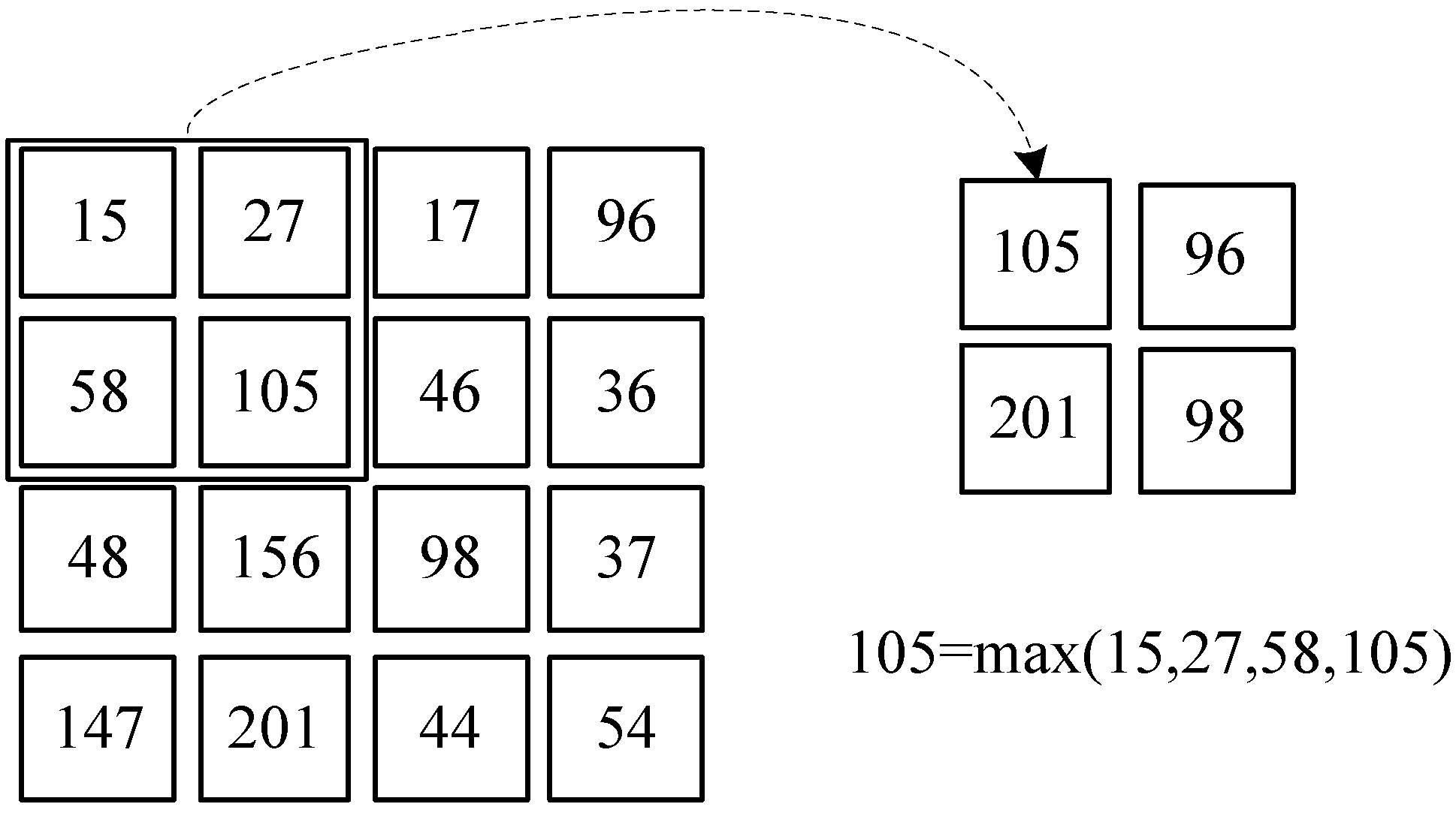
The pool layer, also called the down sample layer, reduces feature map redundancy and network computation complexity by reducing the feature map dimensions and effectively prevents over fitting. The formula for calculating the pooling layer is shown in Equation (3).
where is the jth feature map output by the nth layer convolution layer, is the pooling method, commonly used is the average pooling and maximum pooling, and is the activation function.
When the pooling step size is 2, the process of 2 × 2 maximum pooling is shown in the Figure 1.
2.1.3. Fully-Connected Layer
The full connection is generally placed at the end of the convolutional neural network and the high-level two-dimensional feature map extracted by the previous convolutional layer is converted into a one-dimensional feature map output. In the fully connected layer, each of its neurons is connected to all neurons of the previous layer and there is no weight sharing.
2.2. Depthwise Separable Convolution
In recent years, in order to run high-quality CNN models on mobile terminals with strict memory and computing budgets, many innovative network models have been proposed, such as MobileNet and ShuffleNet. These models include depthwise separable convolution which effectively reduces the amount of parameters and calculations of the network under limited loss of precision.
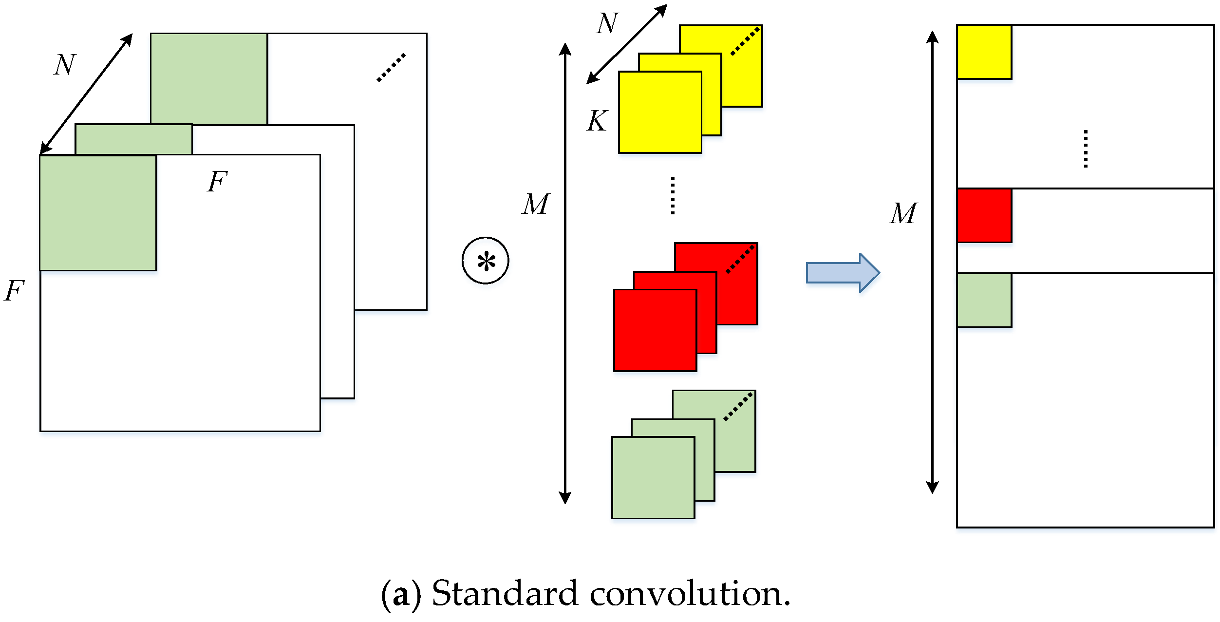
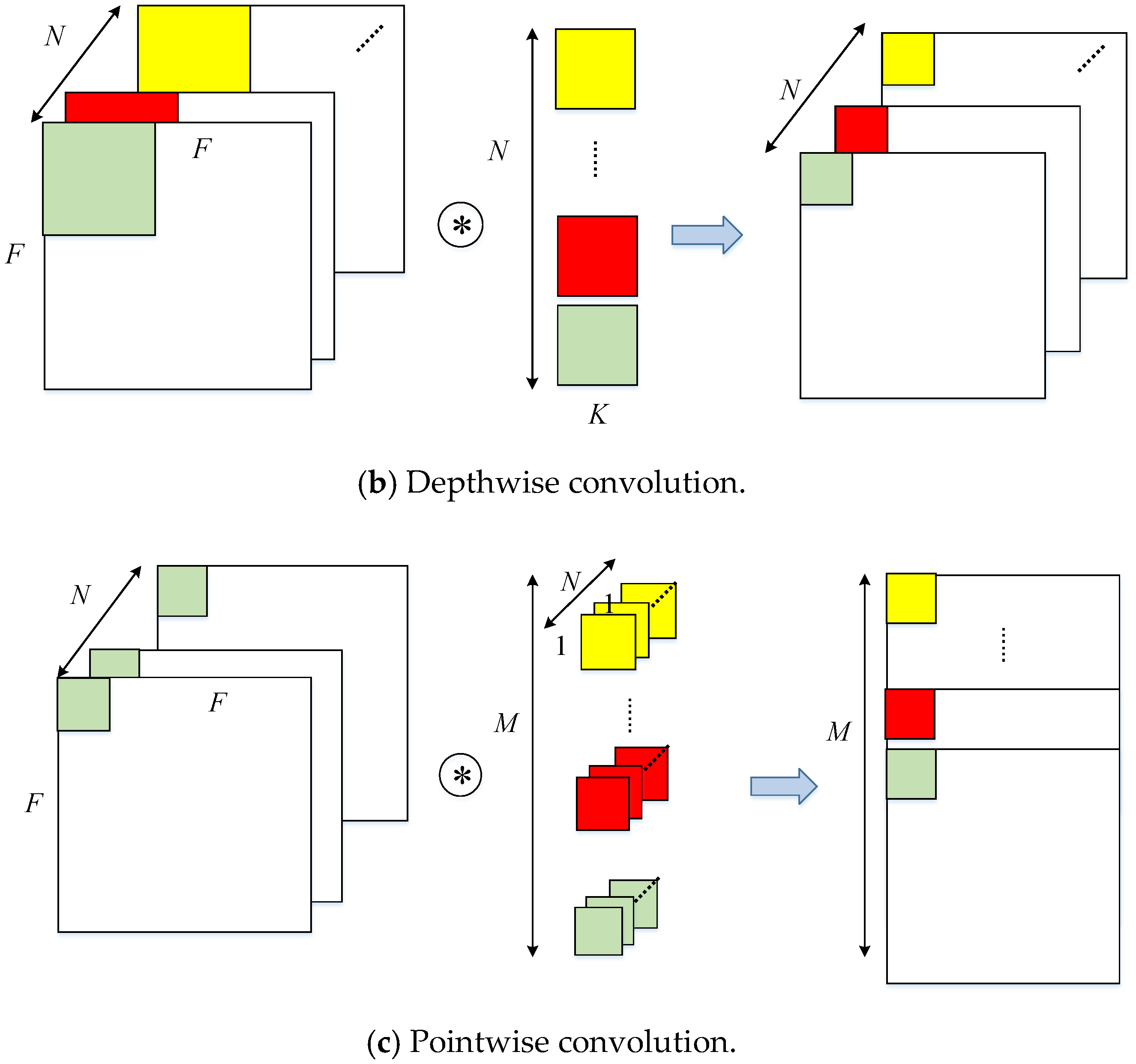
The standard convolution uses a convolution kernel with the same channels of input data to sum a result after channel-by-channel convolution. As Figure 2 shows, depthwise separable convolution is divided into depthwise convolution and pointwise convolution. The former refers to the use of a set of two-dimensional (channel number is 1) kernels to perform the convolution for each channel between input feature maps and kernels individually. The latter is equivalent to the standard convolution of 1 × 1 kernel size. In the following text, it is implemented as a standard convolution.
Assuming that the size of the input feature map is , the size of the convolution kernel is and the stride is 1. The parameter quantities of the standard convolution layer are:
The amount of calculation is:
The parameter quantities of depthwise separable convolution are:
The amount of calculation is:
Thus, the reduction factors on weights and operation are calculated in Equation (8):
3. Architecture and Accelerator Design
In the AI application scenario, the CPU is highly flexible, however not computationally efficient, and the accelerator is computationally efficient, however not flexible enough. Therefore, the architecture that is currently widely used for deep learning usually combines a CPU with an accelerator, called a heterogeneous system. We choose the Xilinx ZYNQ 7100 heterogeneous chip as the hardware platform to complete the design of the system architecture and accelerator.
3.1. Design Overview
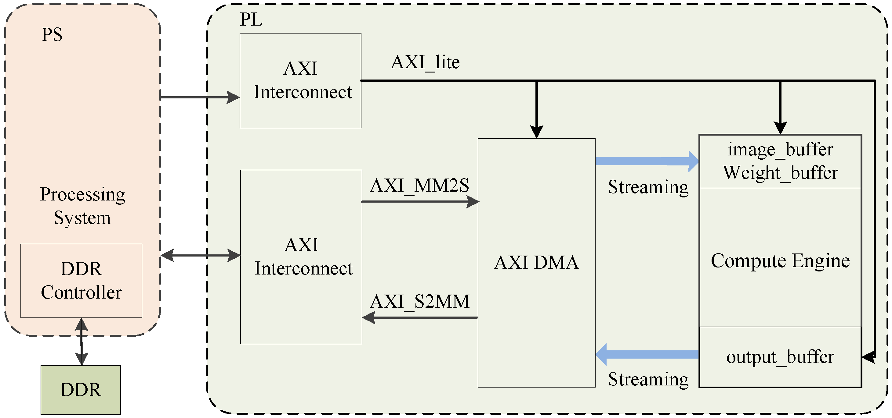
There are currently two different implementation modes for CNN due to its hierarchical structure; one is Streaming Architectures and the other is Single Computation Engine. The former which allocates corresponding hardware resources to each network layer has the following three characteristics: (1) it can realize inter-layer parallelism and flexibly control the parallelism within each layer. (2) It is highly customized and inflexible. (3) The demand for resources is high and only applies to small networks. The latter means that different network layers share the same accelerator through resource reuse, which is a non-highly customized architecture, is more flexible, and is easier to migrate between platforms. Therefore, considering the limited resources of the hardware platform and the parallelism of fully developing the single-layer network structure, we design the system architecture in the single computation engine mode, as shown in Figure 3.
The system architecture mainly includes external memory Double Data Rate (DDR), processing system (PS), on-chip buffer, accelerator in programmable logic (PL), and on-chip and off-chip bus interconnection. The initial image data and weights are pre-stored in the external memory DDR. PS and PL are interconnected through the AXI4 bus. The accelerator receives configuration signals from the CPU through the AXI4_Lite bus (e.g., convolution kernel size, stride, performs standard convolution or depthwise convolution, etc.). Under the action of the DDR controller in the PS, the weight and input data of the current layer required by the accelerator are read from the DDR and are converted from the AXI4_memory map format to the AXI4_streaming format into the on-chip buffer of the accelerator under the action of the Direct Memory Access (DMA). The buffer of the IP core uses the AXI4_Streaming interface and the ping-pong mode. One buffer acts as a producer for receiving data from the DMA and the other is used to participate in the current calculation of the IP core, called a consumer. In the next stage, the producer and the consumer swap. After being processed by the accelerator, the output is sent back to the DDR through the AXI4 bus and the above operation is repeated until the calculation of the entire network model is completed.
It can be seen that the accelerator has two data exchanges with the external memory under the architecture, including receiving the weights and input feature map and sending output feature map back to the off-chip. Frequent data exchange imposes high requirements on the bandwidth of the platform. Therefore, taking the MobileNet + SSD as an example, use the roofline model to jointly consider the computing platform resources and storage bandwidth to seek optimal design for the accelerator.
3.2. Accelerator Design under the Roofline Model
3.2.1. Accelerator Overview
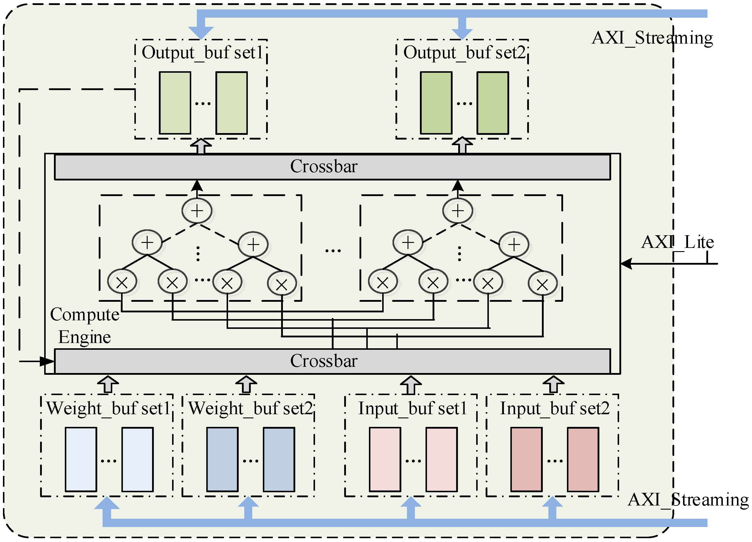
The structure of the accelerator is shown in Figure 4. The on-chip buffer is divided into three parts (1) Input buffer for storing input feature map, (2) Weights buffer for storing weights, (3) Output buffer for storing intermediate results and the output feature map. In order to maximize the external storage bandwidth, the three all use AXI_Streaming interfaces and the ping pong mode. The three processes of inputting input feature map data and weights, calculating convolution, and outputting the calculation result are completely flowed. The compute engine can be selected to work in standard convolution or depthwise convolution modes under the control of the CPU through the AXI_Lite bus.
3.2.2. The Roofline Model of ZYNQ 7100
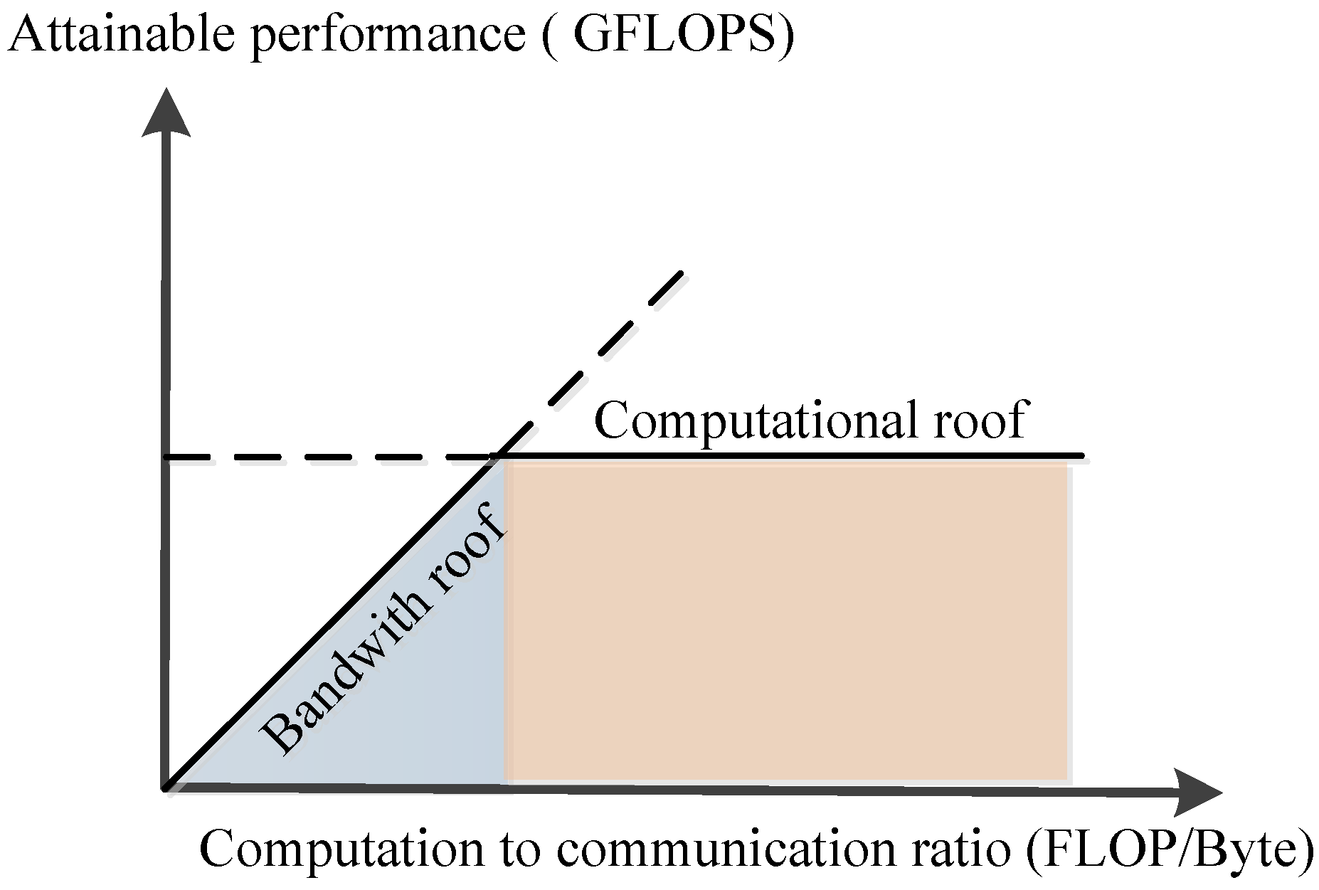
In order to solve the performance prediction problem of the deep learning model on a specific hardware platform, in [27], the roofline model proposed a method of quantitative analysis using operational intensity, which calculates how fast the floating point calculation speed can be achieved under the limitation of external storage bandwidth and computing resources on a hardware platform. This is shown in Figure 5.
Equation (9) formulates the attainable throughput of an application on a specific hardware platform. Giga floating-point operations per second (GFLOPS) is a measure of computing performance. The roofline is divided into two regions: compute bound and memory bound. The computational performance achievable on the platform by the network model cannot exceed the minimum of the two regional bottlenecks. In the case of compute bound, the bottleneck is the computing roof (i.e., a computing platform exhausts all the floating-point operations that can be completed per second). When in the memory bound, the bottleneck is multiplied by the computing to communication (CTC) ratio (i.e., operations per DRAM traffic) and the I/O memory bandwidth (BW),
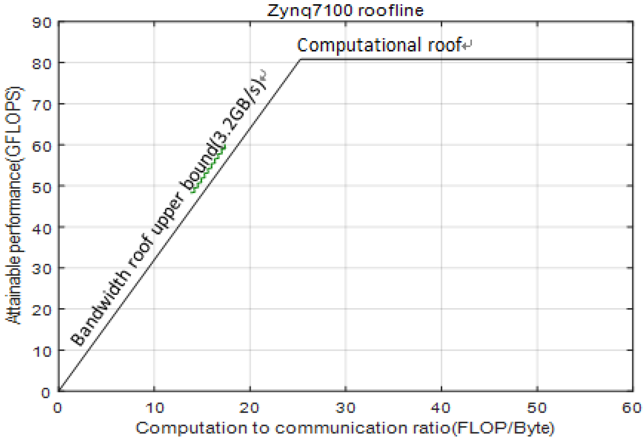
In our work, we calculate the computational roof and the I/O memory maximum bandwidth roof of the Xilinx ZYNQ 7100 computing platform according to Equation (10).
where is the number of hardware platform DSP divided by 5 because it requires five DSPs to complete a multiplication and addition operation of 32-bit floating-point multiply. is the number of High Performance (HP) ports and is the system clock frequency (assumed to be 100 MHz). The constructed skeleton model is shown in Figure 6.
3.2.3. Data Partition and Exploring the Design Space
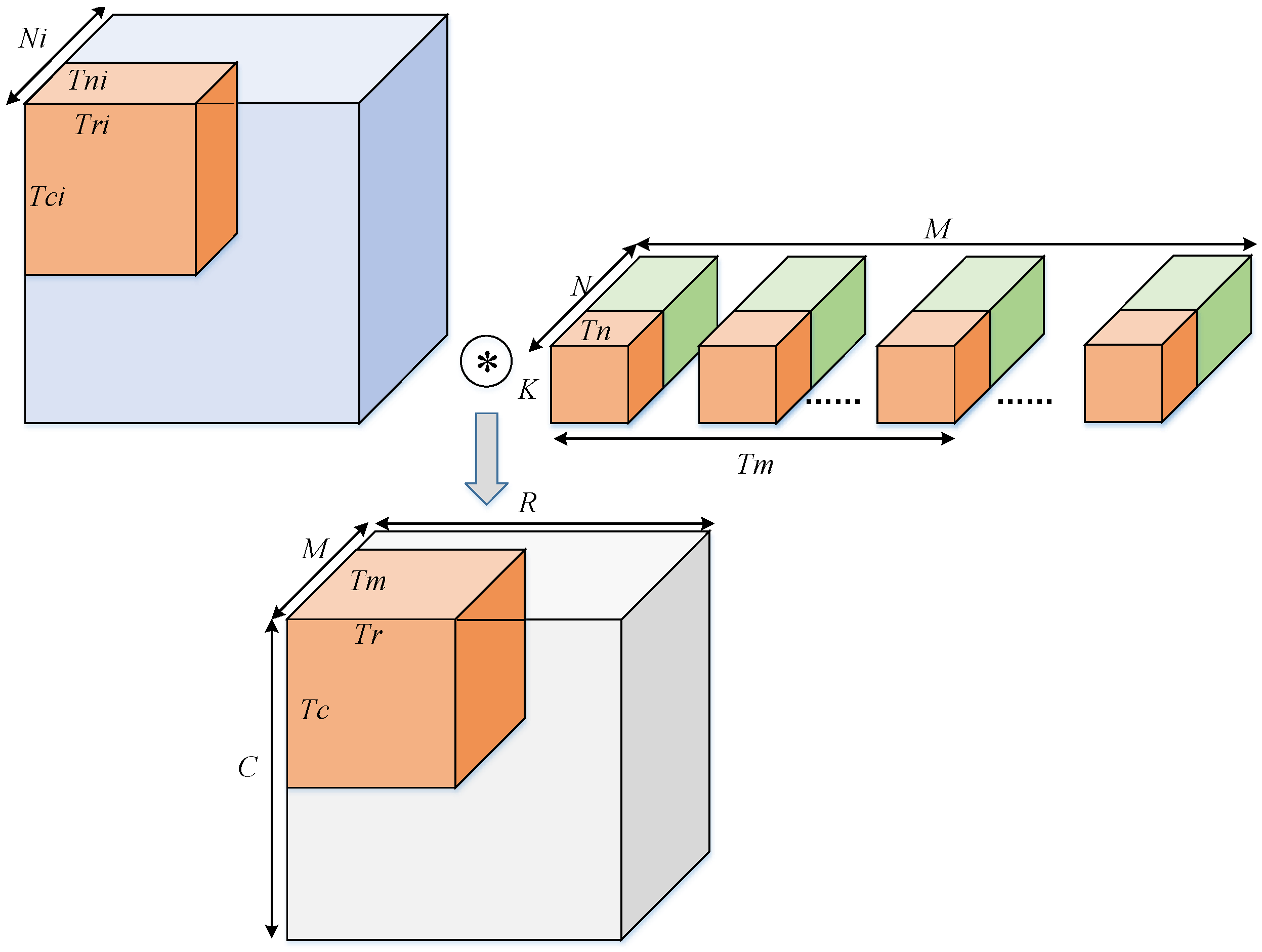
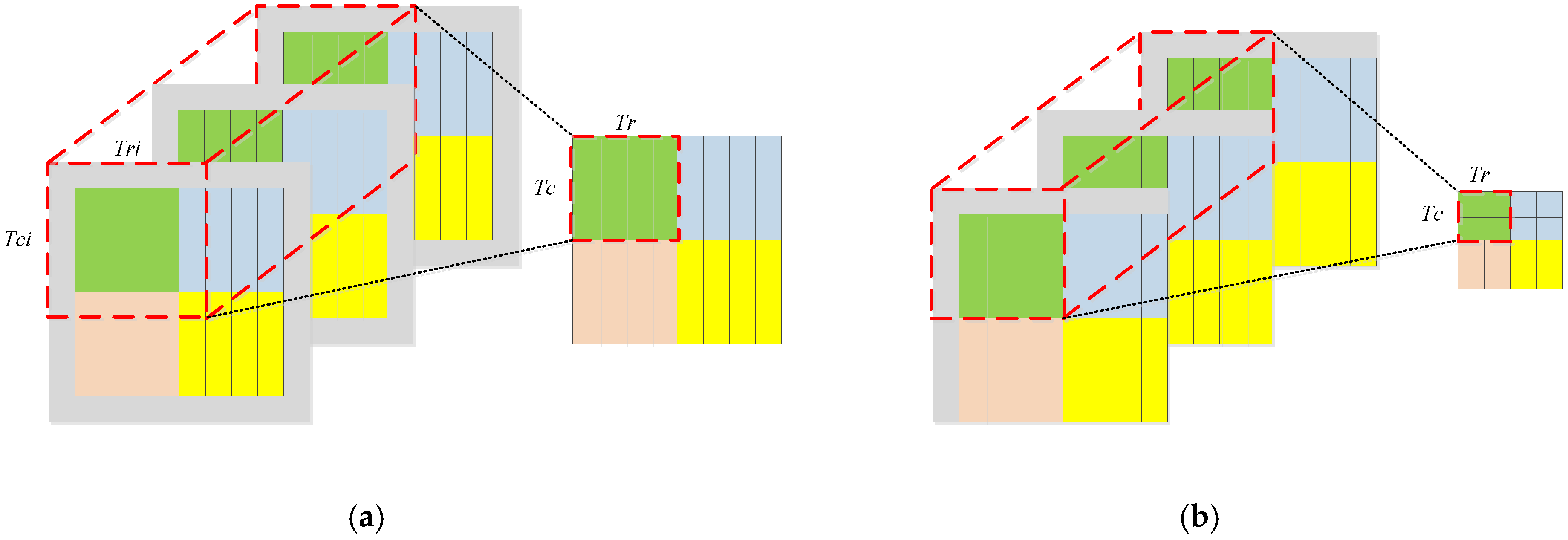
Since the on-chip cache resources are often extremely limited, this is usually unsatisfactory for all input feature maps and weights to be cached on the chip. The data must be partitioned. As shown in Figure 7, since the convolution kernel size itself is small, it is not divided in this dimension. , and are the width, height, and number of convolution kernels of the output feature map (also the number of channels of the output feature map), the channels of convolution kernel channels, and the channels of the input feature map, respectively. , , , and are the block factors of width, height of output feature map, the number and channels of convolution kernels, respectively. , , and are the block factors width, height, and channels of the input feature map, respectively. The above-mentioned block coefficient setting takes into account both standard convolution and depthwise convolution.
We use the example in Figure 8 to illustrate how block convolution works. In this example, the input tensor consists of three separated channels of size 8 × 8 with additional zero padding, the kernel size is 3 × 3, and each input feature map is divided into four independent tiles. Since inter-tile dependencies are eliminated in block convolution, it is not possible to obtain an output tile of size 4 × 4 directly from three input tiles at the corresponding position. As shown in Figure 8a, when the stride is 1, an input tile of size 6 × 6 is required to get an output tile of size 4 × 4. In Figure 8b, an input tile of size 5 × 5 is required to get an output tile of size 2 × 2 when the stride is 2. In block convolution, the relationship between and can be determined as Equation (11):
Block convolution affects the external memory access of the model, which affects the . See Equation (12), which establishes a mathematical connection between the block factors and .
In particular, for standard convolution, and ; however, for depthwise convolution, , and .
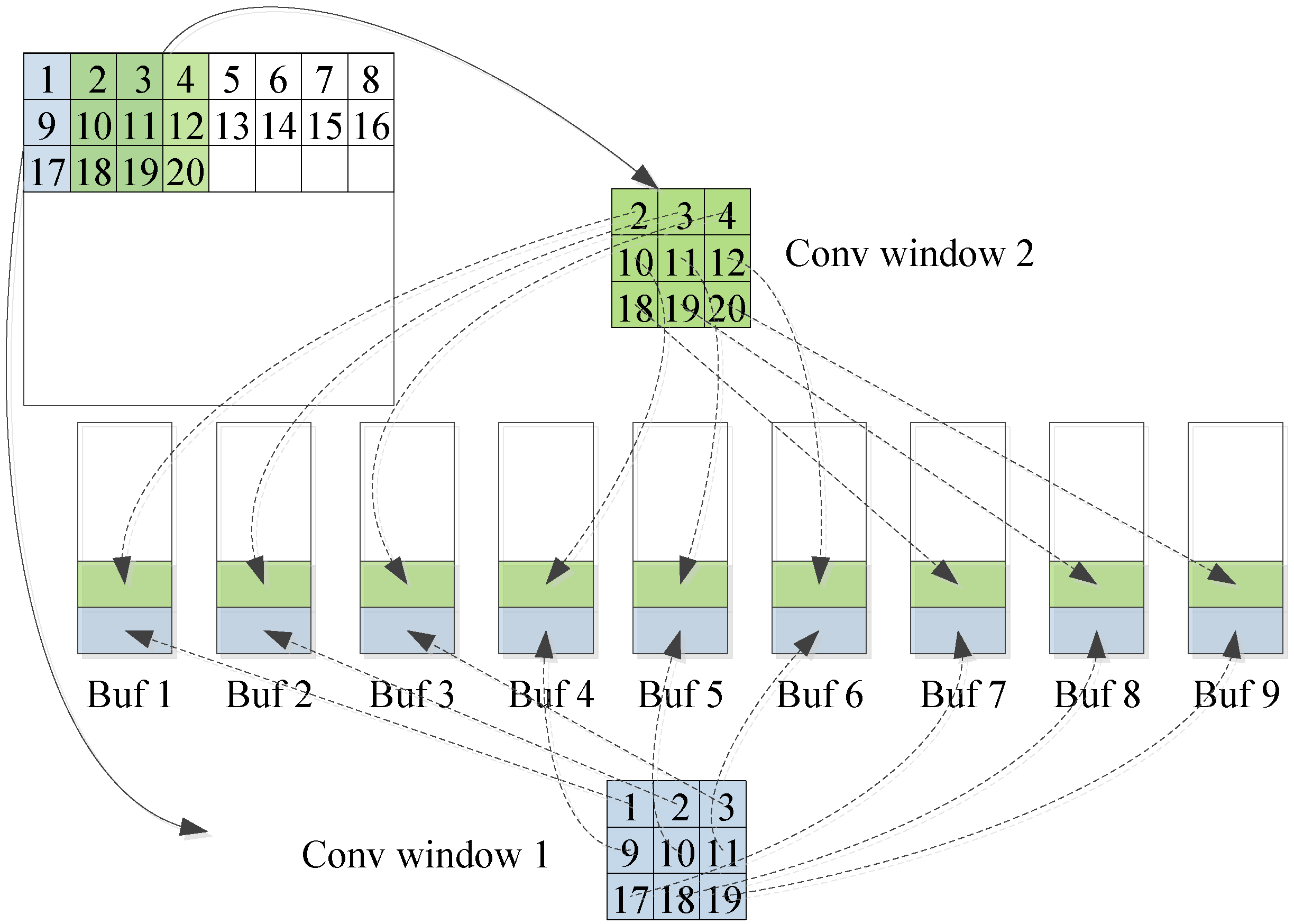
The hardware acceleration effect of CNN depends largely on the degree of development of algorithm parallelism. CNN belongs to a feedforward multi-layer network and its interlayer structure, intra-layer operation, and data stream drive all have certain similarities. Therefore, the convolutional neural network topology CNN itself has many parallelisms. This mainly includes (1) multi-channel operation of the input feature map and convolution kernel. (2) The same convolution window and different convolution kernels can simultaneously perform convolution operations. (3) Multiple convolution windows and the same convolution kernel can simultaneously perform convolution operations. (4) In a convolution window, the parameters corresponding to all convolution kernels of all neuron nodes and corresponding parameters can be operated simultaneously. The above four parallelisms correspond to the dimensions of , , , and , respectively. Computational parallel development not only has certain requirements for computing resources, yet also requires an on-chip cache structure to provide the data needed for parallel computing. However, it also increases the on-chip cache bandwidth. The Vivado HLS development tool makes it very easy to partition an array in a particular dimension. However, if the parallelism of (3) and (4) is developed, the cache structure of the data is shown in Figure 9.
As can be seen from the figure, if the data in a convolution window is to be distributed and stored in buffers, the data is not continuous in the dimension. Vivado HLS is difficult to implement this with array partitioning. Moreover, it repeatedly stores the overlapping data between the convolution windows which greatly increases the consumption of on-chip cache resources. Therefore, we will develop the parallelism of the calculations on the dimensions and .
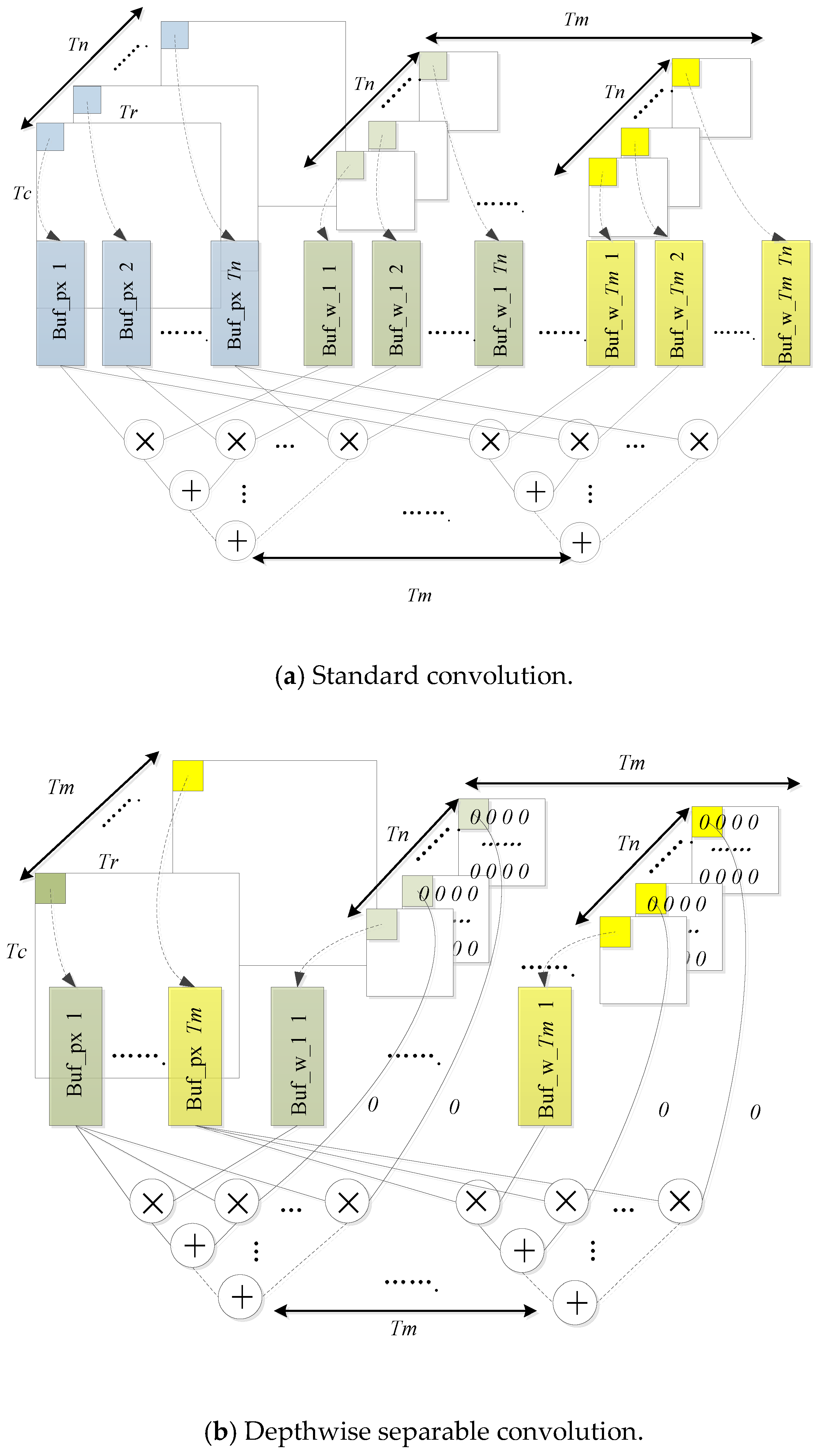
The calculation engine diagram is shown in Figure 10. When calculating the standard convolution, the channels of the input feature map are simultaneously multiplied by the weights of the corresponding channels and then the intermediate results are continuously accumulated which will greatly reduce the delay by pipeline. At the same time, the same operation of the group among different convolution kernels is performed. When dealing with depthwise convolution, channels of the convolution kernel are filled with zero to in order to efficiently integrate the two kinds of convolution and to not destroy the computational parallelism, as shown in Figure 10b.
It can be seen from the above analysis that under the calculation engine we designed, can be calculated by the Equation (13) for a given block factors of , , , and .
Due to array partition and ping-pong buffers, the consumption of on-chip cache resources is increased. To associate the on-chip buffer with the block factors, we need to satisfy Equation (14).
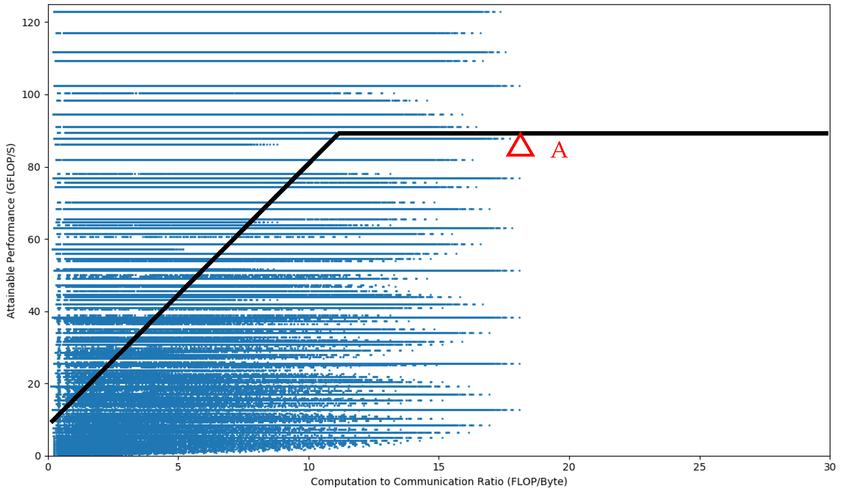
Combining the above-mentioned , , and the analyzed on-chip cache relationship with the roofline model of the ZYNQ 7100 under the block factors of , , , and , we seek the best design and find the optimal block factor, as shown in point A of the Figure 11, under some certain constraints, as shown in Equation (15).
According to the above ideas, the optimal block factors , , , and of the current network layer can be obtained by programming with Matlab. However, the optimal block coefficients obtained from the different layers are different. In particular, and affect the computational parallelism. If and are allowed to be variable, complex hardware architectures need to be designed to support reconfiguration of computational engines and interconnects. So, we will solve the global optimal and under the whole network model, as shown in Formula (16).
where is the number of network layers. and are the minimum and maximum values of sought by all network layers. and are the minimum and maximum values of sought by all network layers.
The final global optimal solution is obtained:
Since Tn and Tm have been determined, the configurable parameters of the accelerator are shown in Table 1.
4. Experimental Evaluation and Results
The accelerator is implemented with Vivado HLS (v2016.4). Vivado HLS (v2016.4) can implement the accelerator in C++ and convert it to the RTL as a Vivado’s IP core which greatly shortens the development cycle. The C code design of the accelerator can be implemented by adding the HLS-defined pragma of Vivado HLS to achieve the parallelism described previously, such as pipeline, array partition, dataflow, and so on. After that, the IP core is imported into the Vivado (v2016.4) project to complete the synthesis and verification on FPGA.
4.1. Resource Utilization
The hardware resources consumed by the accelerator are shown in Table 2.
It can be seen from the table that the implemented accelerator has a high hardware resource rate and also verifies the analysis results of the previous design exploration and computational parallelism.
4.2. Comparisons of Pipelined and no Pipelined
MoblieNet+SSD has a total of 47 network layers which contains both standard convolution and depthwise separable convolution. We use the first network layer that is the standard convolution and the second network layer that is depthwise convolution as the example to compare the running time of full pipelined and no pipelined combined with layer parameters for more details. Table 3 is the parameter of the two network layers. A more detailed comparison is as shown in Table 4 and Table 5, respectively.
The parameters and structure of the network layer are different and the calculation throughput is also different. The performance bottleneck of MobileNet + SSD is the bandwidth roof rather than the computation roof. Therefore, the latency of the full-flow state achieved by the stream data and the ping-pong technique is greatly reduced. Combining the resource report, the pipelined version has higher energy efficiency than the version of not pipelined.
4.3. Comparisons with CPU Implementation
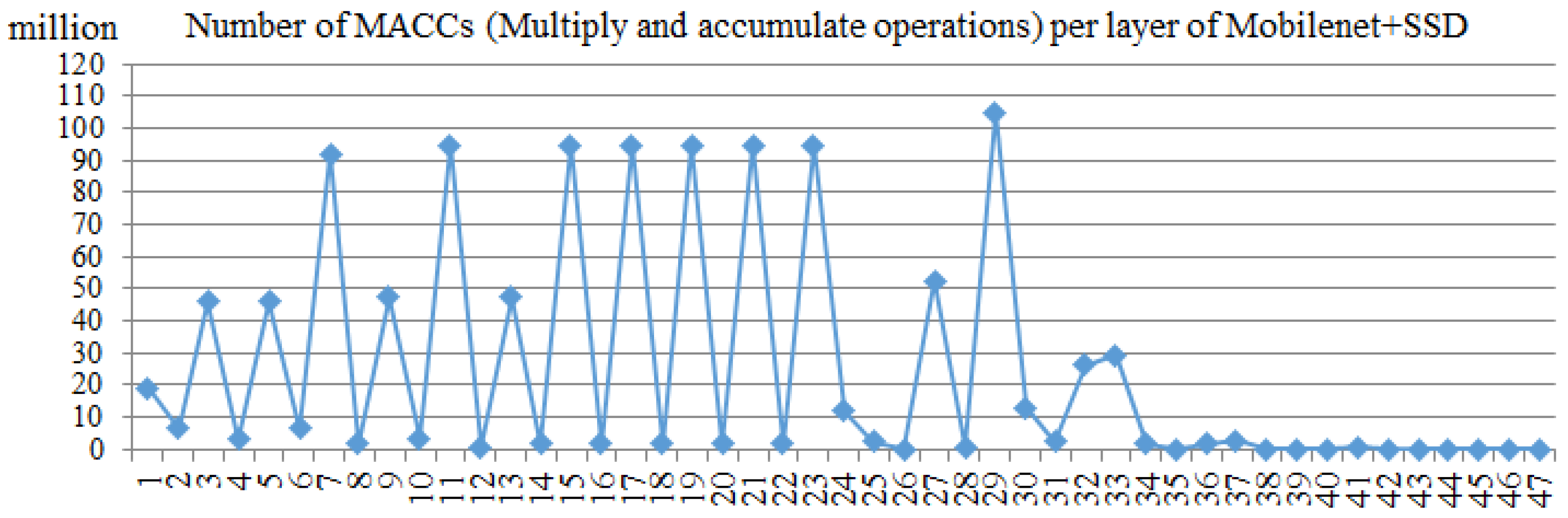
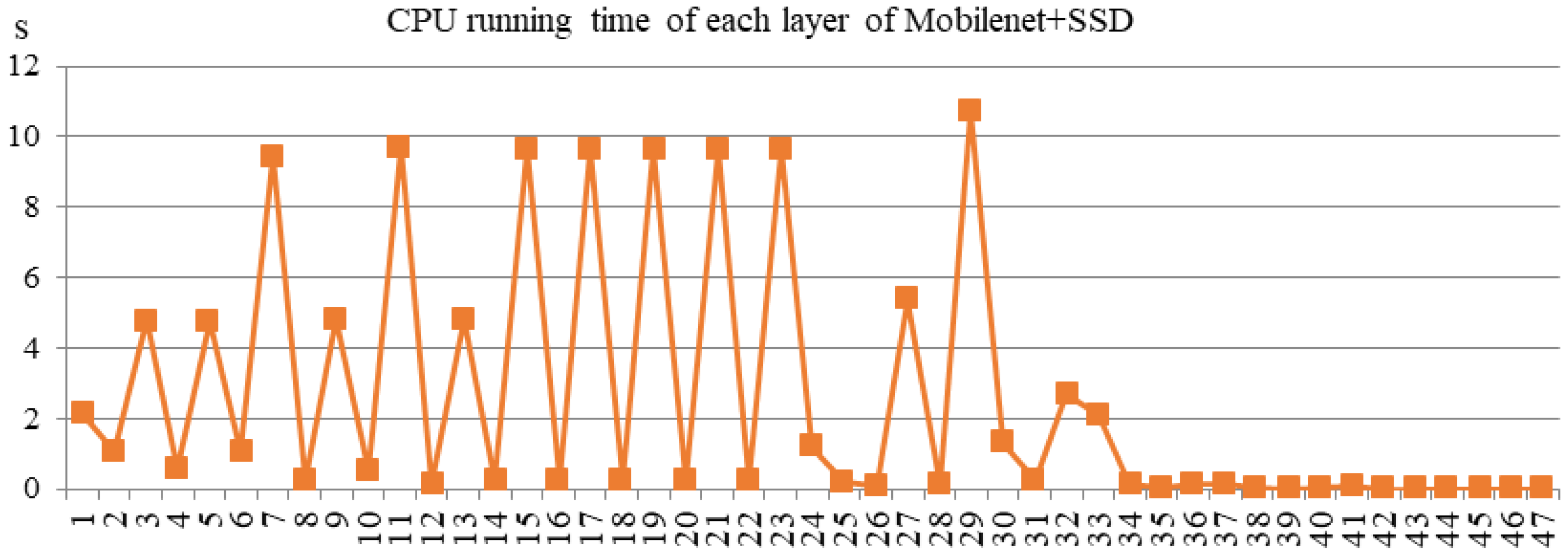
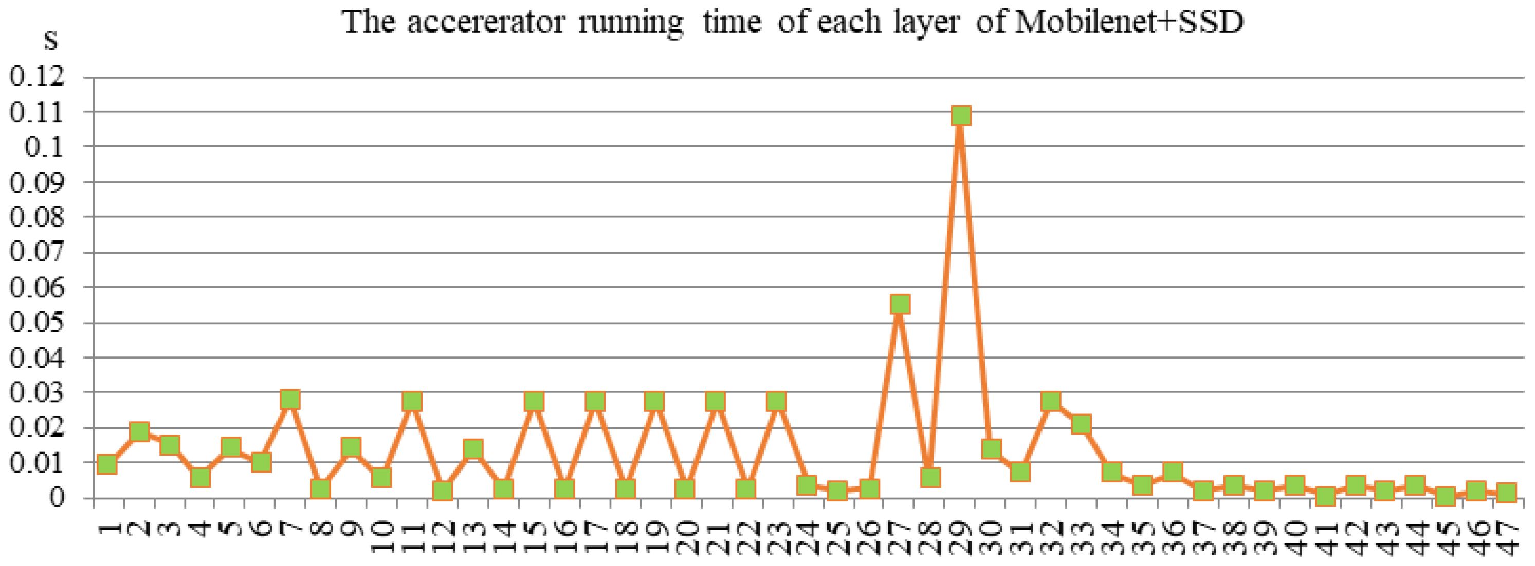
The CPU version is completed by the Cortex-A9 core of ZYNQ 7100. The complier is “arm_xilinx_eabigcc” in Xilinx Software Development Kit. And the software version of -O3 compilation flags is used to compare with an accelerator. The calculation amount of each layer is shown as Figure 12. The running time results of using the CPU and accelerator to complete the MobileNet + SSD network are shown as Figure 13 and Figure 14, respectively.
The running time of each layer in Figure 13 and Figure 14 includes the time fetching the data from the external memory, computing, and sending the results to the external memory with each layer. Combining Figure 13 and Figure 14, it indicates that the time consumption of the accelerator is considerably smaller, more than 150 times faster compared with the software process.
4.4. Comparisons with Others
Compare our implementation of the accelerator with other FPGA-based accelerators, as shown in Table 6.
Since one Multiply-Accumulate (MACC) contains two operations, we convert the performance indicators into (Giga operations per second) GOPS and compare them. Other accelerator implementations do not include depthwise separable convolution, so the performance of our standard convolution is involved in the comparison. If using a fixed-point calculation engine, our method can better perform because the fixed-point processing unit uses fewer resources. It can be seen that the accelerator we have achieved has certain performance advantages.
5. Conclusions
In this article, we implemented a CNN accelerator on the Xilinx ZYNQ 7100 hardware platform that accelerates both standard convolution and depthwise separable convolution. Thanks to the heterogeneous mode of ZYNQ, the accelerator based on the single-computing engine mode can realize network layer acceleration of different scales under the configurable architecture we designed. Taking the MobileNet + SSD network design as an example, the accelerator modeled the global optimal computational parallelism parameter of the entire network under the roofline model of ZYNQ 7100. In order to maximize bandwidth and reduce the delay caused by on-chip off-chip data exchange, the three stream buffers on the chip use the data stream interface and set the ping-pong buffer mode. Even when dealing with standard convolution or depthwise separable convolution, the above-mentioned technology achieves a full pipelined state with a much slower delay than the no pipelined state. In the end, the accelerator achieved a computing performance of 17.11GFLOPS at a clock frequency of 100 MHz and high resource utilization, which is superior to previous designs. Our current system clock frequency is only 100 MHZ, which is lower than other designs. If we can increase the system clock, the performance of the accelerator will be significantly improved.
Author Contributions
Funding: J.L.; Investigation, D.Z.; Methodology, B.L.; Resources, P.F.; Experiment, D.Z. and S.F.; Formal analysis, L.F.; Writing-original draft, D.Z.; Writing-review and editing, B.L. and S.F.
Funding
This research was funded by the National Natural Science Foundation of China under Grant No. 61671170, the Open Projects Program of National Laboratory of Pattern Recognition under Grant No.201700019.
Acknowledgments
The authors would like to thank the Editor and the anonymous reviewers for their valuable comments and suggestions.
Conflicts of Interest
The authors declare no conflict of interest.
Abbreviations
The following abbreviations are used in this manuscript:
| CNN | Convolutional Neural Network |
| FPGA | Field Programmable Gate Array |
| IoT | Internet of Things |
| GPU | Graphics Processing Unit |
| ASIC | Application-Specific Integrated Circuit |
| Open CL | Open Computing Language |
| DDR | Double Data Rate |
| AXI | Advanced eXtensible Interface |
| DRAM | Dynamic Random Access Memory |
| PS | Processing System |
| PL | Programmable Logic |
| DMA | Direct Memory Access |
| HP | High Performance |
| GFLOPS | Giga FLoating-point Operations Per Second |
| CTC | Computing To Communication |
| BW | BandWidth |
| DSP | Digital Signal Processing |
| FF | Flip Flop |
| LUT | Look-Up-Table |
| MACC | Multiply-Accumulate |
| RTL | Register Transfer Level |
References
- Sivaramakrishnan, R.; Sema, C.; Incheol, K.; George, T.; Sameer, A. Visualization and Interpretation of Convolutional Neural Network Predictions in Detecting Pneumonia in Pediatric Chest Radiographs. Appl. Sci. 2018, 8, 1715. [Google Scholar] [CrossRef]
- Yinghua, L.; Bin, S.; Xu, K.; Xiaojiang, D.; Mohsen, G. Vehicle-Type Detection Based on Compressed Sensing and Deep Learning in Vehicular Networks. Sensors 2018, 18, 4500. [Google Scholar] [CrossRef]
- Krizhevsky, A.; Sutskever, I.; Hinton, G.E. ImageNet classification with deep convolutional neural network. Commun. ACM 2017, 60, 84–90. [Google Scholar] [CrossRef]
- Ren, S.; He, K.M.; Girshick, R.; Sun, J. Faster R-CNN: Towards Real-time object Detection with Region Proposal Network. IEEE Trans. Pattern Anal. Mach. Intell. 2017, 39, 1137–1149. [Google Scholar] [CrossRef] [PubMed]
- Abdel-Hamid, O.; Mohamed, A.R.; Jiang, H.; Penn, G. Applying convolutional neural networks concepts to hybrid NN-HMM model for speech recognition. In Proceedings of the 2012 IEEE International Conference on Acoustics, Speech and Signal Processing (ICASSP), Kyoto, Japan, 25–30 March 2012; pp. 4277–4280. [Google Scholar]
- Farabet, C.; Poulet, C.; Han, J.Y.; Le, C.Y. CNP: An FPGA-based processor for convolutional networks. In Proceedings of the International Conference on Field Programmable Logic and Applications, Prague, Czech Republic, 31 August–2 September 2009; pp. 32–37. [Google Scholar]
- Sankaradas, M.; Jakkula, V.; Cadambi, S.; Chakradhar, S.; Durdanovic, I.; Cosatto, E.; Graf, H.P. A massively parallel coprocessor for convolutional neural networks. In Proceedings of the IEEE International Conference on Application-specific Systems, Architectures and Processors, New York, NY, USA, 6–7 July 2009; pp. 53–60. [Google Scholar]
- Hadsell, R.; Sermanet, P.; Ben, J.; Erkan, A.; Scoffier, M.; Kavukcuoglu, K.; Muller, U.; Le, C.Y. Learning long-range vision for autonomous off-road driving. J. Field Robot. 2009, 26, 120–144. [Google Scholar] [CrossRef] [Green Version]
- Maria, J.; Amaro, J.; Falcao, G.; Alexandre, L.A. Stacked autoencoders using low-power accelerated architectures for object recognition in autonomous systems. Neural Process Lett. 2016, 43, 445–458. [Google Scholar] [CrossRef]
- Wei, Z.; Zuchen, J.; Xiaosong, W.; Hai, W. An FPGA Implementation of a Convolutional Auto-Encoder. Appl. Sci. 2018, 8, 504. [Google Scholar] [CrossRef]
- Zhiling, T.; Siming, L.; Lijuan, Y. Implementation of Deep learning-Based Automatic Modulation Classifier on FPGA SDR Platform. Elecronics 2018, 7, 122. [Google Scholar] [CrossRef]
- Han, S.; Liu, X.; Mao, H.; Pu, J.; Pedram, A.; Horowitz, M.A.; Dally, W.J. EIE: Efficient inference engine on compressed deep neural network. In Proceedings of the 2016 International Symposium on Computer Architecture, Seoul, Korea, 18–22 June 2016; pp. 243–254. [Google Scholar]
- Chen, T.S.; Du, Z.D.; Sun, N.H.; Wang, J.; Wu, C.Y.; Chen, Y.J.; Temam, O. DianNao: A small-footprint high-throughput accelerator for ubiquitous machine-learning. ACM Sigplan Notices 2014, 49, 269–284. [Google Scholar]
- Song, L.; Wang, Y.; Han, Y.H.; Zhao, X.; Liu, B.S.; Li, X.W. C-brain: A deep learning accelerator that tames the diversity of CNNs through adaptive data-level parallelization. In Proceedings of the 53rd Annual Design Automation Conference, Austin, TX, USA, 5–9 June 2016. [Google Scholar]
- Andrew, G.H.; Menglong, Z.; Bo, C.; Dmitry, K.; Weijun, W.; Tobias, W.; Marco, A.; Hartwing, A. Mobile Nets: Efficient convolutional neural networks for mobile vision applications. arXiv, 2017; arXiv:1704.04861. [Google Scholar]
- Mark, S.; Andrew, G.H.; Menglong, Z.; Andrey, Z.; Liangchied, C. Mobile Net V2: Inverted residuals and linear bottlenecks. arXiv, 2018; arXiv:1801.04381v3. [Google Scholar]
- Cadambi, S.; Majumdar, A.; Becchi, M.; Chakradhar, S.; Graf, H.P. A programmable parallel accelerator for learning and classification. In Proceedings of the 19th international conference on Parallel architectures and compilation techniques, Vienna, Austria, 11–15 September 2010; pp. 273–284. [Google Scholar]
- Chakradhar, S.; Sankaradas, M.; Jakkula, V.; Cadambi, S. A dynamically configurable coprocessor for convolutional neural networks. In Proceedings of the 37th International Symposiumon Computer Architecture, St Mal, France, 19–23 June 2010; pp. 247–257. [Google Scholar]
- Peemen, M.; Setio, A.A.; Mesman, B.; Corporaal, H. Memory-centric accelerator design for convolutional neural networks. In Proceedings of the 2013 IEEE 31st International Conference (ICCD), Asheville, NC, USA, 6–9 October 2013; pp. 13–19. [Google Scholar]
- Alhamali, A.; Salha, N.; Morcel, R. FPGA-Accelerated Hadoop Cluster for Deep Learning Computations. In Proceedings of the 2015 IEEE International Conference on Data Mining Workshop (ICDMW), Atlantic City, NJ, USA, 14–17 November 2015; pp. 565–574. [Google Scholar]
- Bettoni, M.; Urgese, G.; Kobayashi, Y.; Macii, E.; Acquaviva, A. A Convolutional Neural Network Fully Implemented on FPGA for Embedded Platforms. In Proceedings of the 2017 New Generation of CAS (NGCAS), Genoa, Italy, 6–9 September 2017. [Google Scholar]
- Mousouliotis, P.G.; Panayiotou, K.L.; Tsardoulias, E.G.; Petrou, L.P.; Symeonidis, A.L. Expanding a robot’s life: Low power object recognition via fpga-based dcnn deployment. In Proceedings of the 2018 7th International Conference on Modern Circuits and Systems Technologies (MOCAST), Thessaloniki, Greece, 7–9 May 2018. [Google Scholar]
- Zhang, C.; Li, P.; Sun, G.; Guan, Y.; Xiao, B.; Cong, J. Optimizing fpgabased accelerator design for deep convolutional neural networks. In Proceedings of the 2015 ACM/SIGDA International Symposium on Field-programmable Gate Arrays, Monterey, CA, USA, 22–24 February2015. [Google Scholar]
- Wang, Z.R.; Qiao, F.; Liu, Z.; Shan, Y.X.; Zhou, X.Y.; Luo, L.; Yang, H.Z. Optimizing convolutional neural network on FPGA under heterogeneous computing framework with OpenCL. In Proceedings of the IEEE Region 10 Conference (TENCON), Singapore, 22–25 November 2016; pp. 3433–3438. [Google Scholar]
- Naveen, S.; Vikas, C.; Ganesh, D.; Abinash, M.; Yufei, M. Throughput-optimized Open CL-based FPGA accelerator for largescale convolutional neural networks. In Proceedings of the 2016 ACM/SIGDA International Symposium on Field-Programmable Gate Arrays, Monterey, CA, USA, 21–23 February 2016; pp. 16–25. [Google Scholar]
- Xu, K.; Wang, X.; Fu, S.; Wang, D. A Scalable FPGA Accelerator for Convolutional Neural Networks. Commun. Comput. Inf. Sci. 2018, 908, 3–14. [Google Scholar]
- Williams, S.; Waterman, A.; Patterson, D. Roofline: An insightful visual performance model for floating-point and multicore architectures. Commun. ACM 2009, 52, 65–76. [Google Scholar] [CrossRef]
Figure 1.
Maxpool.

Figure 2.
Standard convolution and depthwise separable convolution.


Figure 3.
FPGA (field programmable gate array) architecture of system implementation.

Figure 4.
Structure of FPGA accelerator.

Figure 5.
Roofline model.

Figure 6.
The roofline model of ZYNQ 7100.

Figure 7.
Data block diagram.

Figure 8.
An example of block convolution: (a) The stride of convolution is one; (b) The stride of convolution is two.
Figure 8.
An example of block convolution: (a) The stride of convolution is one; (b) The stride of convolution is two.

Figure 9.
Array partitioning in Tr and K dimensions.

Figure 10.
Compute engine diagram.

Figure 11.
Design exploration.

Figure 12.
The calculation amount of MobileNet + SSD.

Figure 13.
CPU running time results.

Figure 14.
Accelerator running time results.


Table 1.
Configurable parameters.
| Parameter | Description |
|---|---|
| width | The width of the input feature map |
| height | The height of the input feature map |
| channels_in | Number of channels of convolution kernels |
| channels_out | Number of channels of the output feature map |
| Tr | Block factor of the width of the output feature map |
| Tc | Block factor of the height of the output feature map |
| Tri | Block factor of the width of the input feature map |
| Tci | Block factor of the height of the input feature map |
| Tni | Block factor of the channels of the intput feature map |
| kernel | The size of convolution kernels |
| stride | The stride of convolution |
| pad | Whether to pad or not |
| depthwise | Whether it is a depthwise convolution or not |
| relu | Whether to relu or not |
| split | Whether it is a split layer (detection layer) or not |
Table 2.
Resource utilization of the accelerator.
| Name | Bram_18k | DSP | FF | LUT | Power (pipelined) | Power (unpipelined) |
|---|---|---|---|---|---|---|
| Total | 708 | 1926 | 187,146 | 142,291 | 4.083 W | 3.993 W |
| Available | 1510 | 2020 | 554,800 | 277,400 | - | - |
| Utilization (%) | 46 | 95 | 38 | 51 | - | - |
Table 3.
Parameter of the two network layers.
| Name | First Layer | First Layer (Block) | Second Layer | Second Layer (Block) |
|---|---|---|---|---|
| Output_fm row (R) | 150 | 150 | 150 | 150 |
| Output_fm col (C) | 150 | 150 | 150 | 150 |
| Output_fm channel (M) | 32 | 64 | 32 | 64 |
| Input_fm channel (Ni) | 3 | 6 | 32 | 64 |
| Kernel channel (N) | 3 | 6 | 1 | 6 |
| Kernel (K) | 3 | 3 | 3 | 3 |
| Stride (S) | 2 | 2 | 1 | 1 |
Table 4.
Comparisons of the first layer.
| Name | No Pipelined | Full Pipelined |
|---|---|---|
| Latency (clock cycles) | 1,921,492 | 934,612 |
| Clock frequency (MHz) | 100 | 100 |
| Time (ms) | 19.21 | 9.35 |
| Calculated amount (GLOPs) | 0.16 | 0.16 |
| Performance (GLOPS) | 8.32 | 17.11 |
Table 5.
Comparisons of the second layer.
| Name | No Pipelined | Full Pipelined |
|---|---|---|
| Latency (clock cycles) | 2,816,722 | 1,904,020 |
| Clock frequency (MHz) | 100 | 100 |
| Time (ms) | 28.2 | 19 |
| Calculated amount (GLOPs) | 0.16 | 0.16 |
| Performance (GLOPS) | 5.67 | 8.42 |
Table 6.
Comparison to previous implementations.
| [7] | [17] | [18] | [19] | Ours | |
|---|---|---|---|---|---|
| Precision | 16 bits fixed | fixed point | 48 bits fixed | fixed point | 32 bits float |
| frequency (MHz) | 115 | 125 | 200 | 150 | 100 |
| FPGA chip | Virtex5 LX330T | Virtex5 SX240T | Virtex5 SX240T | Virtex6 SX240T | ZYNQ 7100 |
| Performance (GMACS) | 3.37 | 3.50 | 8.00 | 8.50 | 8.55 |
| Performance (GOPS) | 6.74 | 7.00 | 16.00 | 17.00 | 17.11 |
© 2019 by the authors. Licensee MDPI, Basel, Switzerland. This article is an open access article distributed under the terms and conditions of the Creative Commons Attribution (CC BY) license (http://creativecommons.org/licenses/by/4.0/).
Share and Cite
MDPI and ACS Style
Liu, B.; Zou, D.; Feng, L.; Feng, S.; Fu, P.; Li, J. An FPGA-Based CNN Accelerator Integrating Depthwise Separable Convolution. Electronics 2019, 8, 281. https://doi.org/10.3390/electronics8030281
AMA Style
Liu B, Zou D, Feng L, Feng S, Fu P, Li J. An FPGA-Based CNN Accelerator Integrating Depthwise Separable Convolution. Electronics. 2019; 8(3):281. https://doi.org/10.3390/electronics8030281
Chicago/Turabian StyleLiu, Bing, Danyin Zou, Lei Feng, Shou Feng, Ping Fu, and Junbao Li. 2019. "An FPGA-Based CNN Accelerator Integrating Depthwise Separable Convolution" Electronics 8, no. 3: 281. https://doi.org/10.3390/electronics8030281
Note that from the first issue of 2016, this journal uses article numbers instead of page numbers. See further details here.