Improved Fractional Open Circuit Voltage MPPT Methods for PV Systems

Abstract

This paper proposes two new Maximum Power Point Tracking (MPPT) methods which improve the conventional Fractional Open Circuit Voltage (FOCV) method. The main novelty is a switched semi-pilot cell that is used for measuring the open-circuit voltage. In the first method this voltage is measured on the semi-pilot cell located at the edge of PV panel. During the measurement the semi-pilot cell is disconnected from the panel by a pair of transistors, and bypassed by a diode. In the second Semi-Pilot Panel method the open circuit voltage is measured on a pilot panel in a large PV system. The proposed methods are validated using simulations and experiments. It is shown that both methods can accurately estimate the maximum power point voltage, and hence improve the system efficiency.

1. Introduction

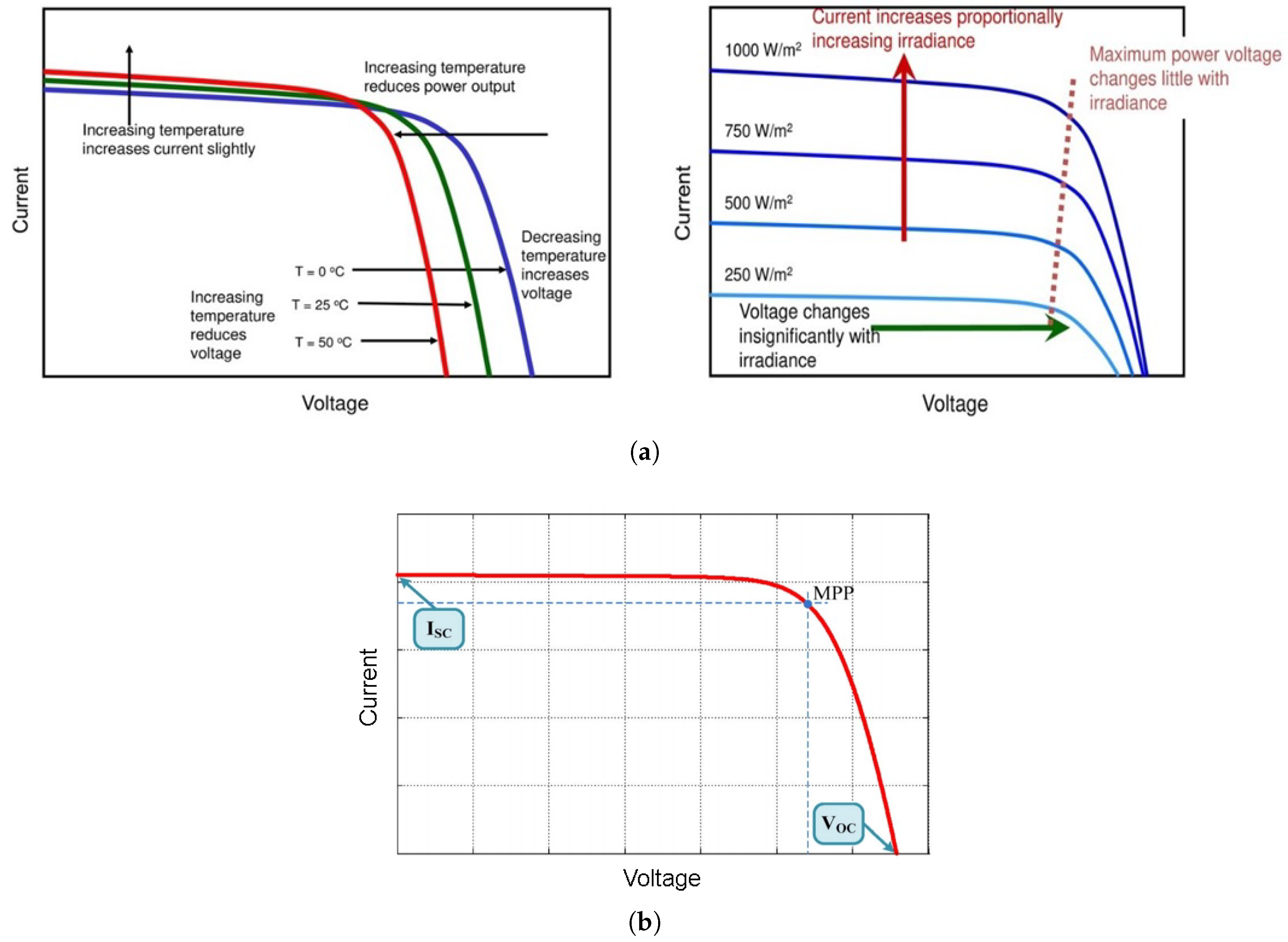
One challenge that frequently arises in photovoltaic (PV) systems is that the output voltage, current and power constantly vary, due to irradiation and temperature changes. Figure 1a shows that the output current is mostly effected by irradiance changes, while the output voltage is mostly effected by temperature changes.

In order to operate the PV array at maximum efficiency it is crucial to extract maximum power from the PV system (Figure 1b). As a result, many Maximum Power Point Tracking (MPPT) methods have been developed in recent years. These methods vary in complexity, type, cost, efficiency, number of sensors, and required hardware. Papers [1,2,3,4,5,6,7,8,9] compare between common MPPT methods and explain the main differences between them. For example, paper [1] compares the efficiency, stability, and quality of different MPPT methods; [2] compares several MPPT methods with respect to the amount of energy extracted from the (PV) panel, tracking factor, PV voltage ripple, dynamic response, and the number of sensors; paper [3] discusses the advantages and drawbacks of different MPPT methods, and provide guidelines for choosing the most suitable MPPT method for a specific PV system; paper [4] compares the Perturb and Observe, Incremental Conductance, Fractional Open Circuit Voltage and Fractional Short Circuit Current methods; [5] presents detailed description and classification of MPPT techniques based on the number of control variables, types of control strategies, types of circuitry, and common practical/commercial applications; [6] presents the general architectures of different MPPT techniques, and discusses their main advantages and disadvantages; [7] presents a detailed survey of artificial neural network MPPT techniques; [8] presents a survey of conventional and advanced MPPT methods, and analyzes the effects of varying meteorological conditions; [9] presents a comparative study of seven common MPPT algorithms.

MPPT methods can be divided into three major categories. The first category includes methods that continuously track the voltage and/or current, without using empirical data. The main advantage of such methods is that they do not require prior knowledge of the PV array characteristics. As a result, these are usually accurate for varying irradiance and temperature. Common MPPT methods associated with this category are Incremental Conductance (IC) [10,11,12,13,14,15,16,17,18,19], Hill Climbing (HC) [20,21,22,23,24,25,26,27,28,29,30], Perturb and Observe (P&O) [31,32,33,34,35,36,37,38], and fuzzy logic techniques [39,40,41,42,43]. The second category includes MPPT methods that calculate the MPP based on apriori data, without continuous tracking the voltage and current. The data often include typical voltage-current curves for different irradiances and temperatures. The main advantage of such methods is that they require less current and/or voltage sensors. However, such methods usually cannot precisely track the MPP for any irradiance and temperature changes. several methods belonging to this category are Fractional Open Circuit Voltage (FOCV) [44], Fractional Short Circuit current (FSCC) [38,45], Curve Fitting [46], and Look-up Tables [47]. The third category includes hybrid methods, that use both measurements and apriori data. For instance, paper [48] presents an MPPT method that uses a Neural Network. Another example is shown in paper [49], which presents a modified Perturb and Observe method with adaptive duty cycle step. All MPPT algorithms are implemented as part of the control circuitry of a DC-DC converter that connects the PV array to the load [50,51].

The Fractional Open Circuit Voltage method, belonging to the second category discussed above, has been explored in several recent works [44,52,53,54,55]. The method is based on the almost linear relationship that exists between the open-circuit voltage-$V_{oc}$ and the $V_{mpp}$ voltage:

$$V_{mpp}=K_{pv}{V}_{oc},$$

(1)

where the constant $K_{pv}$ is the voltage factor. This constant can be calculated based on the panel V-I curves, and is usually in the range 0.7–0.9. Typically this value is specified in the panel’s datasheet. To estimate the $V_{mpp}$ voltage using the FOCV method, the open circuit voltage is measured and multiplied by the voltage factor. The measured open-circuit voltage typically allows an accurate estimation of the $V_{mpp}$ voltage, since the voltage factor remains almost constant for changing irradiance and temperature. The open circuit voltage is periodically sampled by momentarily disconnecting the load. The frequency and duration of the sampling process directly influence the accuracy of the estimated $V_{mpp}$, where high frequency and/or large duty-cycles improves the estimation accuracy, but also increase the power loss.

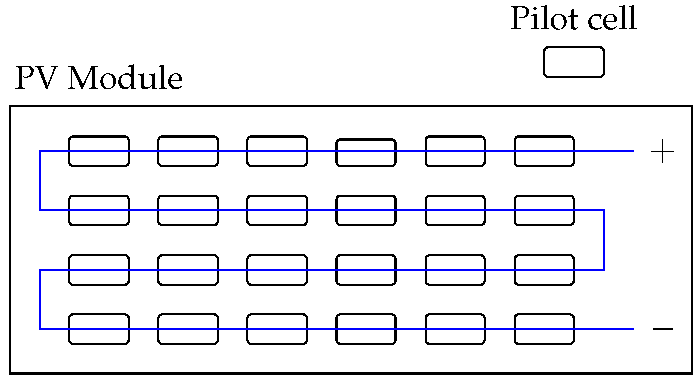
This issue may be solved by using an additional pilot cell, which is similar to other cells in PV array but is used only for open-circuit voltage measurements, as shown in Figure 2. If the pilot cell has the same irradiance and temperature as the other cells then the open circuit voltage can be measured directly, without disconnecting the load. However, since the pilot cell is isolated from the PV panel, it does not produce useful power. The major advantage of the FOCV method in comparison to other common methods such as Incremental Conductance, Perturb and Observe and Hill Climbing are low cost and simple implementation.

Two general challenges of the FOCV method are to improve the accuracy and to reduce the power loss. In this light, this study proposes an improved Fractional Open Circuit Voltage (FOCV) which is an extension to [52]. The main idea is to reduce the power loss during open-circuit voltage measurements by replacing the pilot cell by a semi-pilot cell. During normal operation, the semi-pilot cell is a part of the PV array and contributes to the total generated power. The open-circuit voltage is measured when the semi-pilot cell is disconnected from the array. As a result the power of the semi-pilot cell is lost only when it is disconnected, and not constantly. The measured open-circuit voltage is used by the control circuitry of the DC/DC converter which implements the FOCV MPPT algorithm. The main advantage of the proposed approach is that the semi-pilot cell power is utilized efficiently, and the power supplied to the load is almost unaffected. The main challenges is to properly design the switching period of the semi-pilot cell in order to extract maximum power, and to efficiently track the MPP during and following a switching event.

The paper is organized as follows. Section 2 explains the proposed semi-pilot cell approach. Section 3 explains the simulation setups. Section 4 presents simulation and analysis of the proposed SPC-FOCV method under irradiance and temperature variations. Section 5 discusses the proposed semi-pilot panel SPP-FOCV method. Section 6 shows experimental validation and analysis of the SPP-FOCV method. Conclusions are presented in the last section.

2. The Proposed Semi-Pilot Cell SPC-FOCV Method

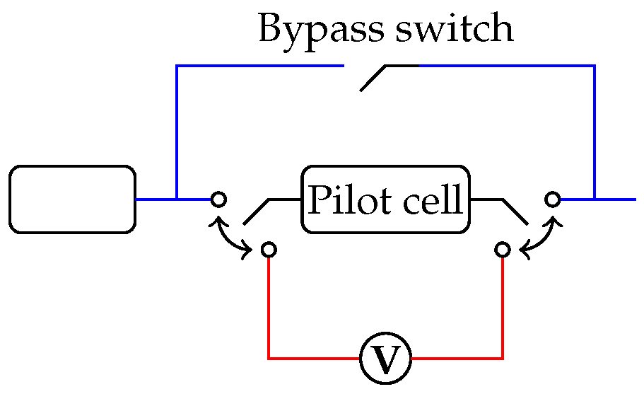
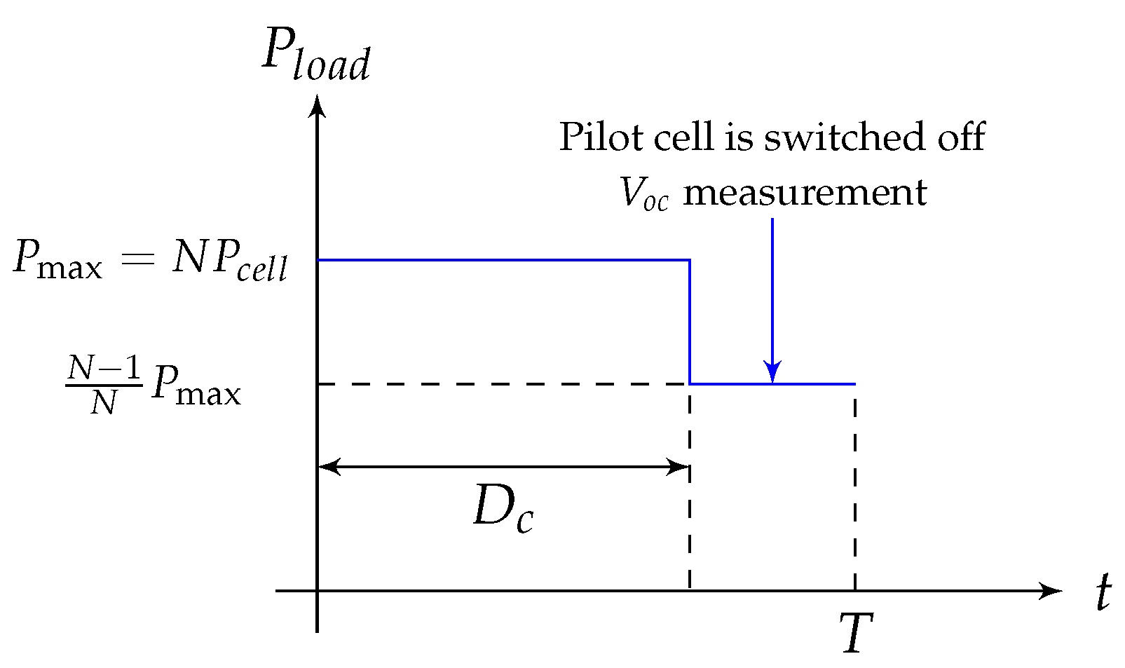
The main purpose of the proposed semi-pilot cell (SPC) FOCV approach is to reduce the power loss in comparison to the conventional FOCV method. The semi-pilot cell is integrated into the PV array and delivers power to the load as other PV cells. However, unlike the other cells, the semi-pilot cell can be disconnected from the PV array in order to measure the open-circuit voltage. The semi-pilot cell operation cycle can be divided into two stages. During the first stage (supply period), there are no measurements of the open circuit voltage and the semi-pilot cell supplies power to the load. During the second stage (measurement period), the semi-pilot cell is disconnected from the array, and the open-circuit voltage is measured, as shown in Figure 3. during this stage the semi-pilot cell is bypassed by a switch, which can be implemented by a MOSFET as shown in Figure 4.

The average power supplied to the load $(P_{\sup })$ over a complete cycle depends on the duty cycle and the number of PV cells in the PV module (see Figure 5) and can be calculated by

$$P_{\sup }=P_1+P_2=P_{\max }{D}_c+\frac{N-1}{N}{P}_{\max }(1-D_c),$$

(2)

where N is the number of cells in the PV array, $P_{\max }$ is the maximal power that can be supplied by the PV, $P_1$ is the supplied power during the first stage, $P_2$ is the supplied power during the second stage, and $D_c$ is the duty cycle of semi-pilot cell switching.

The total power loss of the switches are comprised of conduction and switching losses:

$$\Delta P_{sw}=P_c+P_{sw}.$$

(3)

Note that only the power loss of switch 1 and bypass switch are considered, while losses of switch 2 are neglected since it only connects and disconnects the voltage sensor. The current through switch 2 is zero. The power losses of switch 1 and bypass switch are different because switch 1 is operated with $V_{mpp}$ and $I_{mpp}$ that correspond to n cells while the bypass switch is operated at the MMP that corresponds to $n-1$ cells. The conduction power losses during the operation cycle are calculated by:

$$P_c=P_{c,sw1}{D}_c+P_{c,bp}(1-D_c),$$

(4)

where $P_{c,sw1}$ and $P_{c,bp}$ are the conduction losses of the switch 1 and bypass switch and they can be calculated by:

$$P_{c,sw}=I_D^2{R}_{DS(on)},$$

(5)

where $I_D$ is the current that flows through a Mosfet and $R_{DS(on)}$ is Drain to Source On resistance. The switching losses of each switch can be calculated by:

$$P_{sw}=\frac{I_D{V}_{DD}(t_r+t_f)}{2}{F}_{sw},$$

(6)

where $V_{DD}$ is the voltage that is blocked by the Mosfet, $F_{sw}$ is the switching frequency and $t_r$ and $t_f$ are the rise and fall times respectively. The power that is lost during the open circuit voltage measurement can be calculated as:

$$\Delta P_{meas}=P_{\max }-P_{\sup }.$$

(7)

The total power losses can be calculated by:

$$\Delta P_{tot}=\Delta P_{sw}+\Delta P_{meas}.$$

(8)

The efficiency of the proposed method can be calculated by:

$$\eta =\frac{P_{\sup }-\Delta P_{tot}}{P_{\max }}.$$

(9)

Table 1. Comparison between conventional FOCV, pilot cell FOCV, and proposed semi-pilot cell FOCV methods.

	Conventional	Pilot Cell	Proposed
$P_{\sup }$	$P_{\max }{D}_c$	$P_{\max }$	$P_{\max }{D}_c+\frac{N-1}{N}{P}_{\max }(1-D_c)$
$\Delta P_{meas}$	$P_{\max }(1-D_c)$	$P_{\max }/N$	$P_{\max }-P_{\sup }$
$\Delta P_{sw}$	$P_c{D}_c+P_{sw}$	0	$P_c+P_{sw}$
$\Delta P_{tot}$	$P_{\max }(1-D_c)+P_c{D}_c+P_{sw}$	$P_{\max }/N$	$P_{\max }-P_{\sup }+P_c+P_{sw}$
$\eta$	$(P_{\sup }-\Delta P_{tot})/P_{\max }$	$1-\frac{1}{N}$	$(P_{\sup }-\Delta P_{tot})/P_{\max }$

shows a comparison between the conventional FOCV, pilot cell FOCV, and proposed semi-pilot cell FOCV methods, in terms of output power, power losses and efficiency. The conventional FOCV-MPPT method also uses two Mosfets in order to switch the PV array between the load and the voltage sensor and therefore, the power losses of the switches has to be considered.

It can be seen from this Table that the power losses in the conventional FOCV are directly related to the switches power losses and switching duty cycle i.e., they depend on the duration of the voltage sampling and while the power losses in the pilot cell FOCV are defined only by the output power of the pilot cell. The power losses in the SPC-FOCV depend both on the output power of the semi-pilot cell, the switching duty cycle and switches power losses.

3. Simulation Setup

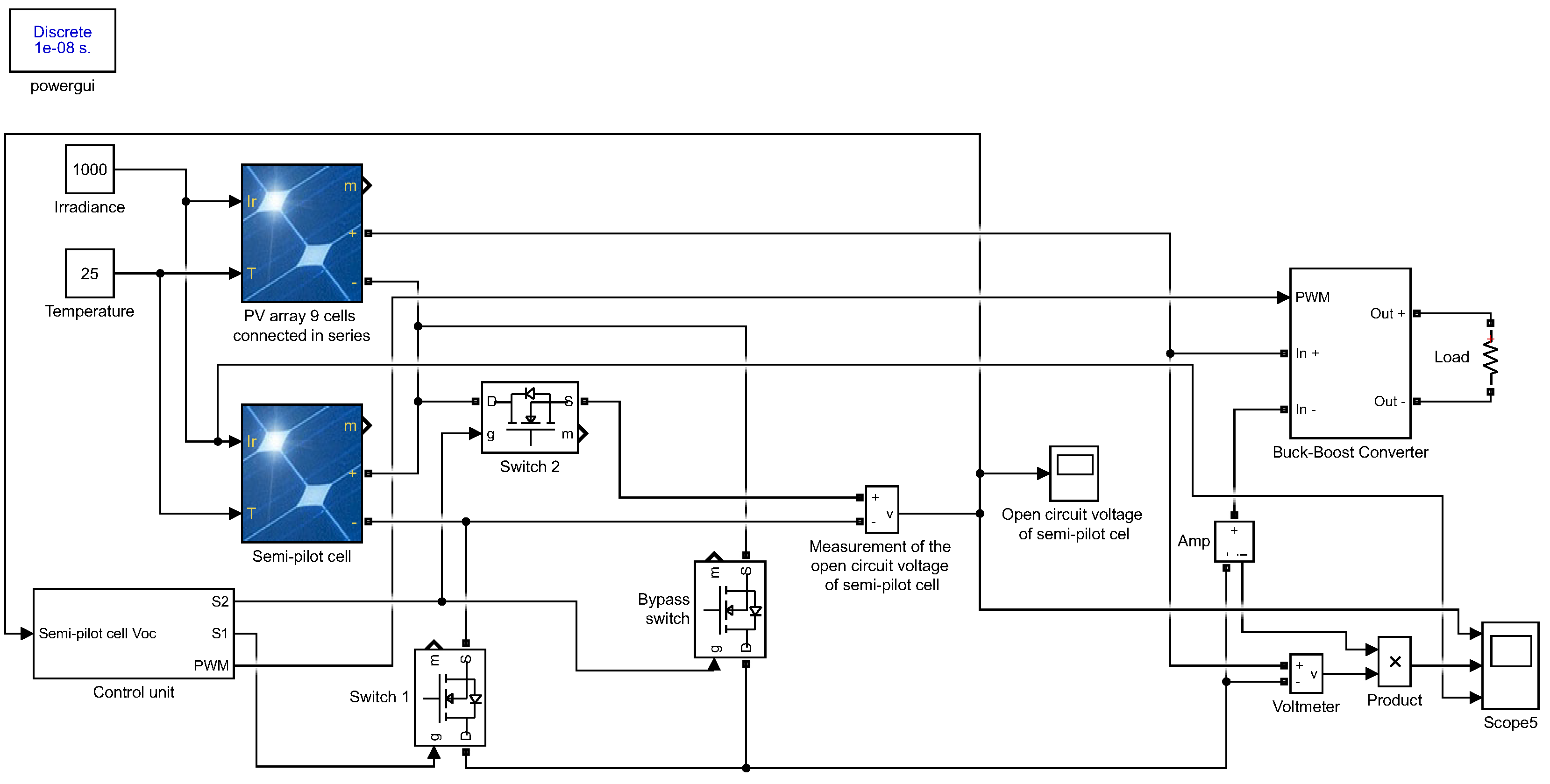
The Simulink simulation setup of the proposed SPC-FOCV method is shown in Figure 6. The accuracy of the simulation is defined by the sample time of 1 × 10⁻⁸ s. The simulated circuit consists of PV array with nine cells connected in series and additional series connected semi-pilot cell. This PV array feeds the load through Buck-Boost DC-DC converter. All cells have similar parameters which are detailed in

Table 2. Simulation parameters.

PV Cell Parameters	Value	Mosfet Parameters	Value
Series resistance [W]	0	$R_{DS(on)}$ resistance [Ω]	0.0064
Short open circuit voltage [V]	0.6	Internal diode forward voltage [V]	0.8
Short circuit current [A]	6	Internal diode resistance [Ω]	0.001
Quality factor	1.5
Nominal temperature [°C]	25

. In this example, temperature of all cells is 25 °C and irradiance is W/m².

Three Mosfet switches are used in order to implement the SPC-FOCV method. Switch 1 is used for semi-pilot cell connection to the array during supply periods and disconnection from the array during measurement periods. Switch 2 connects the semi-pilot cell to voltmeter during measurement periods and disconnects it during supply periods. Bypass switch bypasses disconnected semi-pilot cell during measurement periods in order to allow continuous feeding of the load by the remaining nine cells.

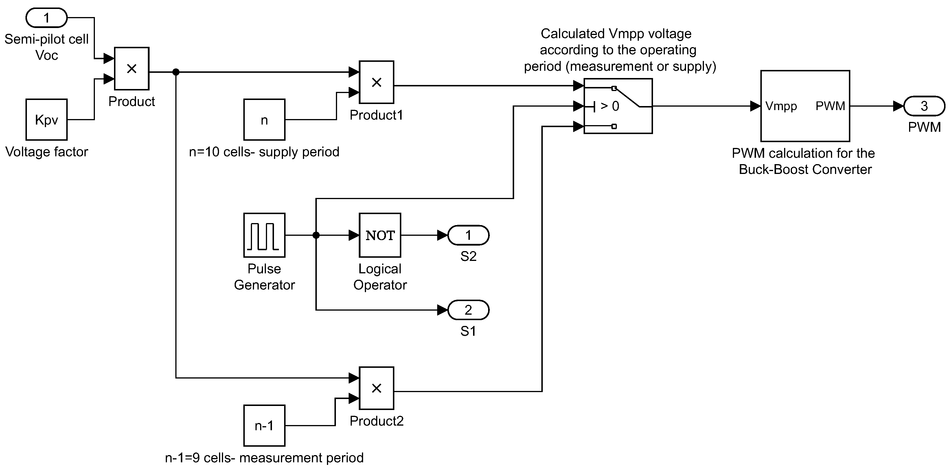
The control unit presented in Figure 7. The main objectives of the control unit are switches operation, calculation of the $V_{mpp}$ voltage according to the corresponding period and PWM signal generation for the Buck-Boost converter. The input of the control unit is measured open circuit voltage of the semi-pilot cell while the outputs are switching signals (S1, S2) for the switches and PWM signal for the Buck-Boost converter.

The switches are operated by the Control unit according to the following principle. During supply periods, switch 1 is closed while switches 2 and bypass are open. During measurement periods, switch 1 is open while switches 2 and bypass are closed. The frequency of the operation cycle and its duty cycle are synchronized by the Pulse generator that supplies switching signal to switch 1 (output S1). The switching signal for switch 2 and bypass switch is obtained by applying “Not” logical operator to the Pulse generator’s signal (output S2).

The $V_{mpp}$ voltage of whole PV array is calculated by multiplication of the measured open circuit voltage of the semi-pilot cell, voltage factor and number of cells. However, the number of cells varies according to the operation period. During supply periods, the number of cells is n ($n=10$ in this example) and therefore, the $V_{mpp}$ voltage is calculated by $V_{mpp}=n{V}_{oc}{K}_{pv}$. During measurement periods, the number of cells is $n-1$ and the $V_{mpp}$ voltage is calculated by $V_{mpp}=(n-1)V_{oc}{K}_{pv}$. To match the calculation of the $V_{mpp}$ voltage to the corresponding period i.e., to the corresponding number of cells, the control unit uses signal switch that is synchronized to the Pulse generator. The signal switch passes through the value of calculated $V_{mpp}$ voltage according to the appropriate operation period. Therefore, the calculated $V_{mpp}$ voltage will vary between the supply and measurement periods.

In each operation period, the Buck-Boost converter is tuned to the calculated $V_{mpp}$ voltage in accordance with the number of cells (n or $n-1$) that are feeding the converter. This will ensure maximum possible output power of the PV array for each operation period. To set the Buck-Boost converter to the calculated $V_{mpp}$ voltage, the control unit generates the corresponding PWM signal that is supplied to the converter.

4. Simulation and Analysis of the Proposed SPC-FOCV Method under Irradiance and Temperature Variations

4.1. SPC-FOCV Operation under Irradiance Variations

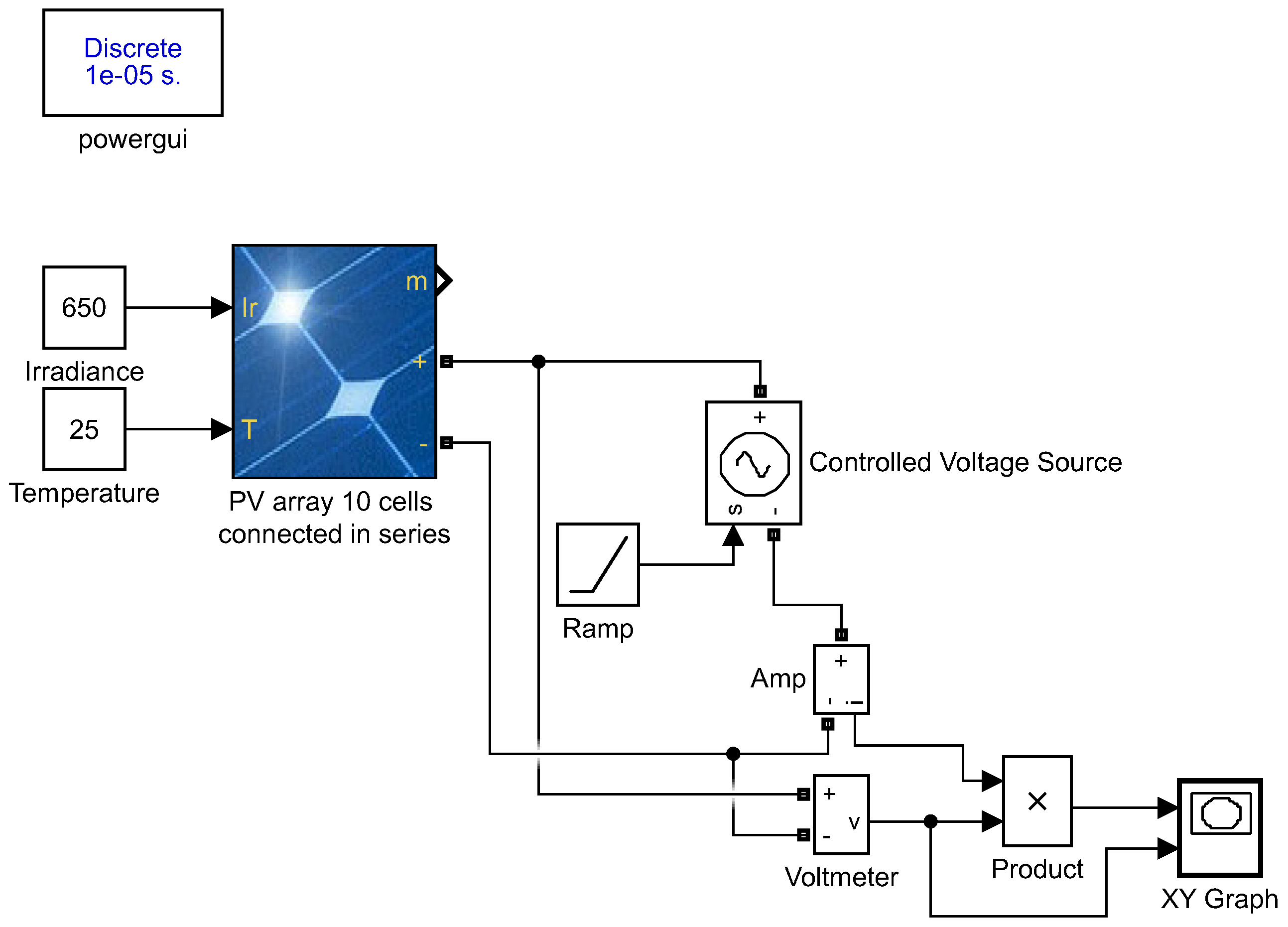
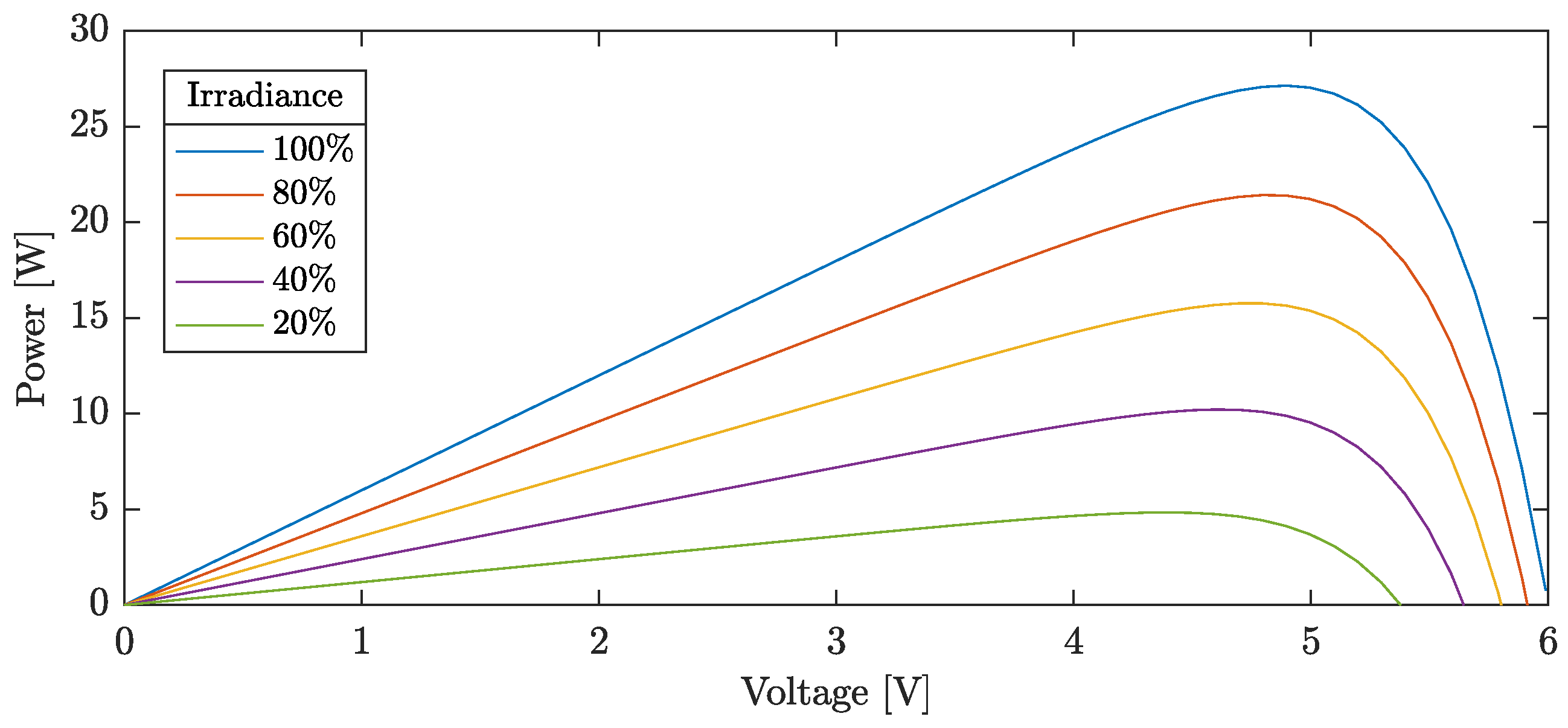
The graph of the simulated PV array’s output power vs. output voltage for constant cells temperature of 25 °C and different irradiance values is shown in Figure 8. The output power vs. output voltage curves are obtained by the simulation circuit shown in Figure 9 where the irradiance of the PV array is changed according to the desired curve i.e., 100%, 80%, etc. The simulated PV array consists of ten series connected cells (the parameters of the cells are shown in Table 2) and feeds the load that is implemented by varying voltage source that is swept between zero to the value (6 V) of the array’s open circuit voltage.

This graph can be used in order to measure the value of the PV array’s $V_{mpp}$ voltage for each specific irradiance. This measured $V_{mpp}$ voltage is for ten series connected cells and corresponds to the supply period.

Before application of the SPC-FOCV method, it is important to know the value of the voltage factor $K_{pv}$ for different irradiance levels. The voltage factor values can be calculated according to (1) or taken from the manufacturer’s datasheet. The calculated voltage factor vs. irradiance is shown in

Table 3. The calculated voltage factor for different irradiance values.

Irradiance [W/m2]	1000	800	600	400	200
$K_{pv}$ (calculated)	0.816	0.816	0.816	0.816	0.815

. It can be seen that the voltage factor is constant for all irradiance values except for values of 200 W/m² and lower, where the voltage factor slightly decreases. Therefore, small error in $V_{mpp}$ estimation is expected for irradiances below 200 W/m².

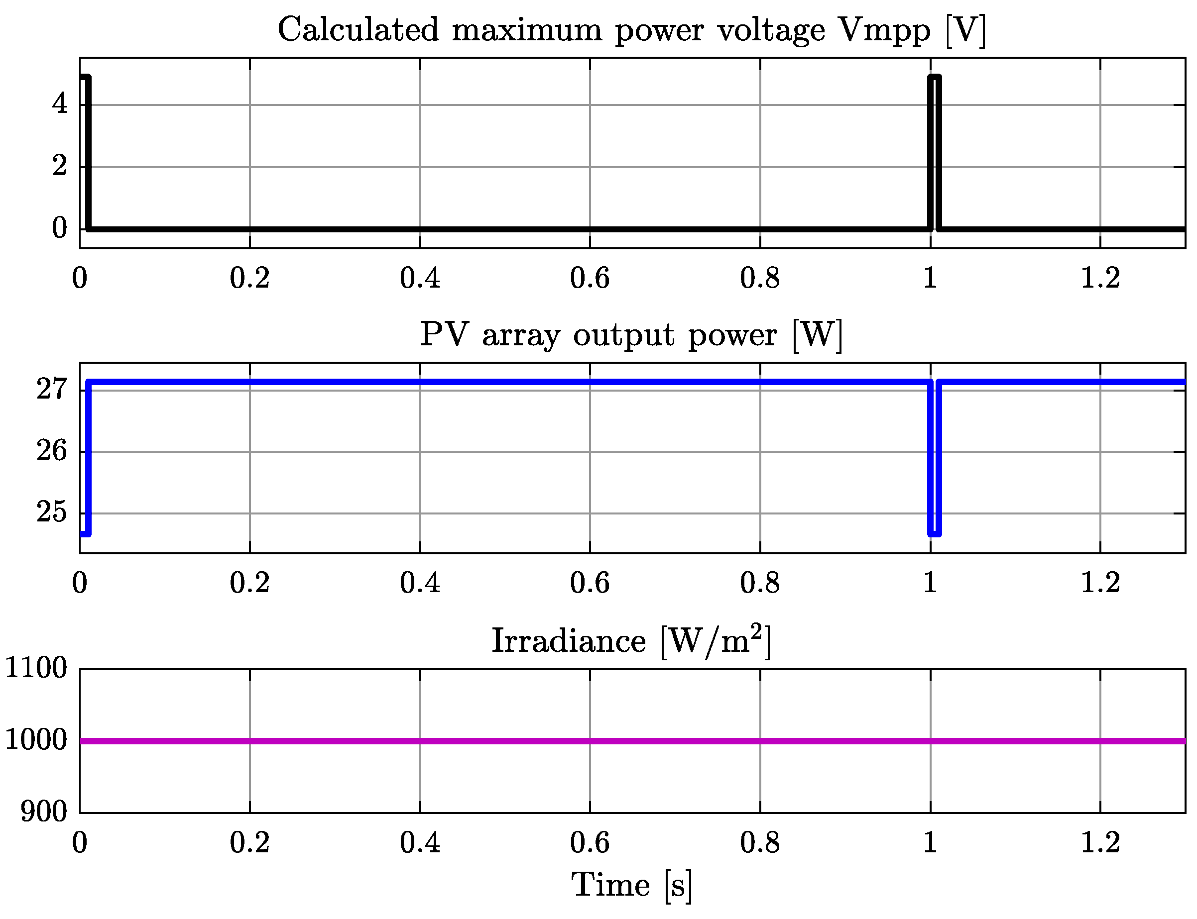
Three different scenarios were simulated and analyzed. The presented simulation results were obtained by the simulation circuit from Figure 6 where irradiance conditions were matched to each scenario. In all three cases, the open circuit voltage measurement on the semi-pilot cell was performed every 0.99 s for 0.01 s (operation cycle is 1 s, $D_c$ = 99%). The temperature of the cells was set to 25 °C. The first scenario corresponds to a sunny day with constant maximal irradiance of 1000 W/m², as shown in Figure 10. During the open circuit voltage measurement periods, the control unit sets the input voltage of the DC-DC converter to the value of the corresponding $V_{mpp}$ voltage that is calculated by multiplication of the semi-pilot’s measured open circuit voltage 0.6 V by the voltage factor 0.816 and by the $n-1=9$ cells: $V_{mpp}=(n-1)V_{oc}{K}_{pv}=4.4$ V. The converter’s operation at the $V_{mpp}=4.4$ V ensures maximal PV array output power during the measurement period. In this scenario the irradiance and temperature conditions are constant. Therefore, in all measurement periods, the measured open circuit voltage of the semi-pilot will have the same value of 0.6 V. When the measurement period ends, the control unit uses previously measured $V_{oc}$ in order to calculate new $V_{mpp}$ voltage that corresponds to n cells: $V_{mpp}=n{V}_{oc}{K}_{pv}=4.896$ V. The control unit sets the input voltage of the DC-DC converter to 4.896 V during the following supply period in order to ensure maximal PV array output power.

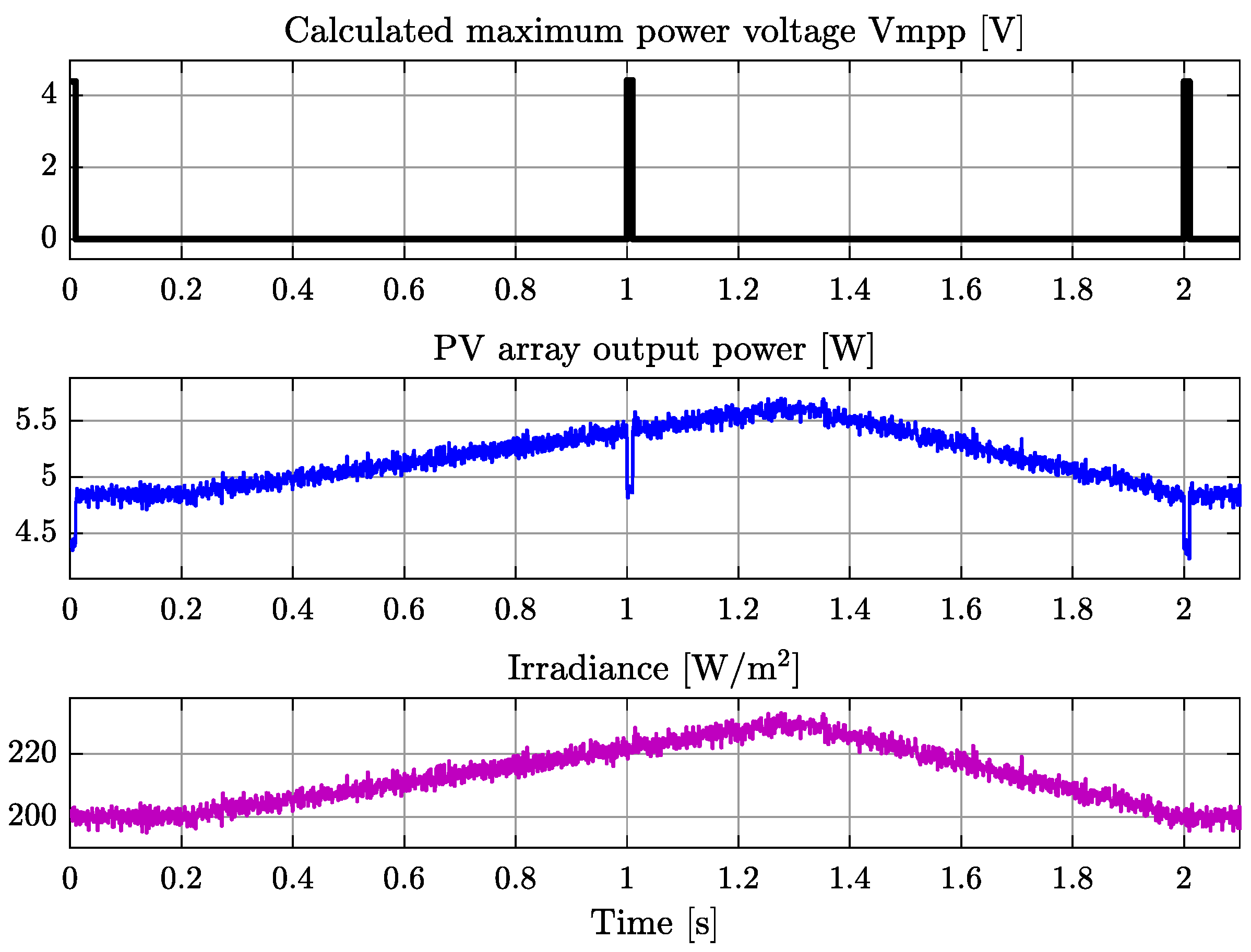
The second scenario simulates cloudy conditions of varying irradiance between 200 to 230 W/m² with randomly generated irradiance noise, as shown in Figure 11. It can be seen from Figure 11 that irradiance noise adds noise to the Pv array’s output power. In the first measurement period between 0–0.01 s, the measured open circuit voltage is 0.538 V. The DC-DC converter is tuned to $V_{mpp}=3.94$ V. In the following supply period between 0.01–1 s the DC-DC converter is tuned to $V_{mpp}=4.38$ V. During this supply period, the irradiance increases but the DC-DC converter remains tuned to 4.38 V until the next measurement period where the $V_{mpp}$ voltage will be updated. Therefore, during the period between 0.2–1 s, the PV array’s output power is 5.36 W (not maximal) instead of 5.39 W (maximal power). The mismatch is very small 0.7%. This mismatch can be avoided by increasing the cycle’s frequency. At the second measurement period between 1–1.01 s, the irradiance was increased to 220 W/m² and the measured open circuit voltage equals 0.542 V. Therefore, the DC-DC converter is tuned to $V_{mpp}=3.97$ V. In the following supply period between 1.01–2 s the DC-DC converter is tuned to $V_{mpp}=4.41$ V. However, the irradiance variations continue and the tuned $V_{mpp}$ is also not maximal.

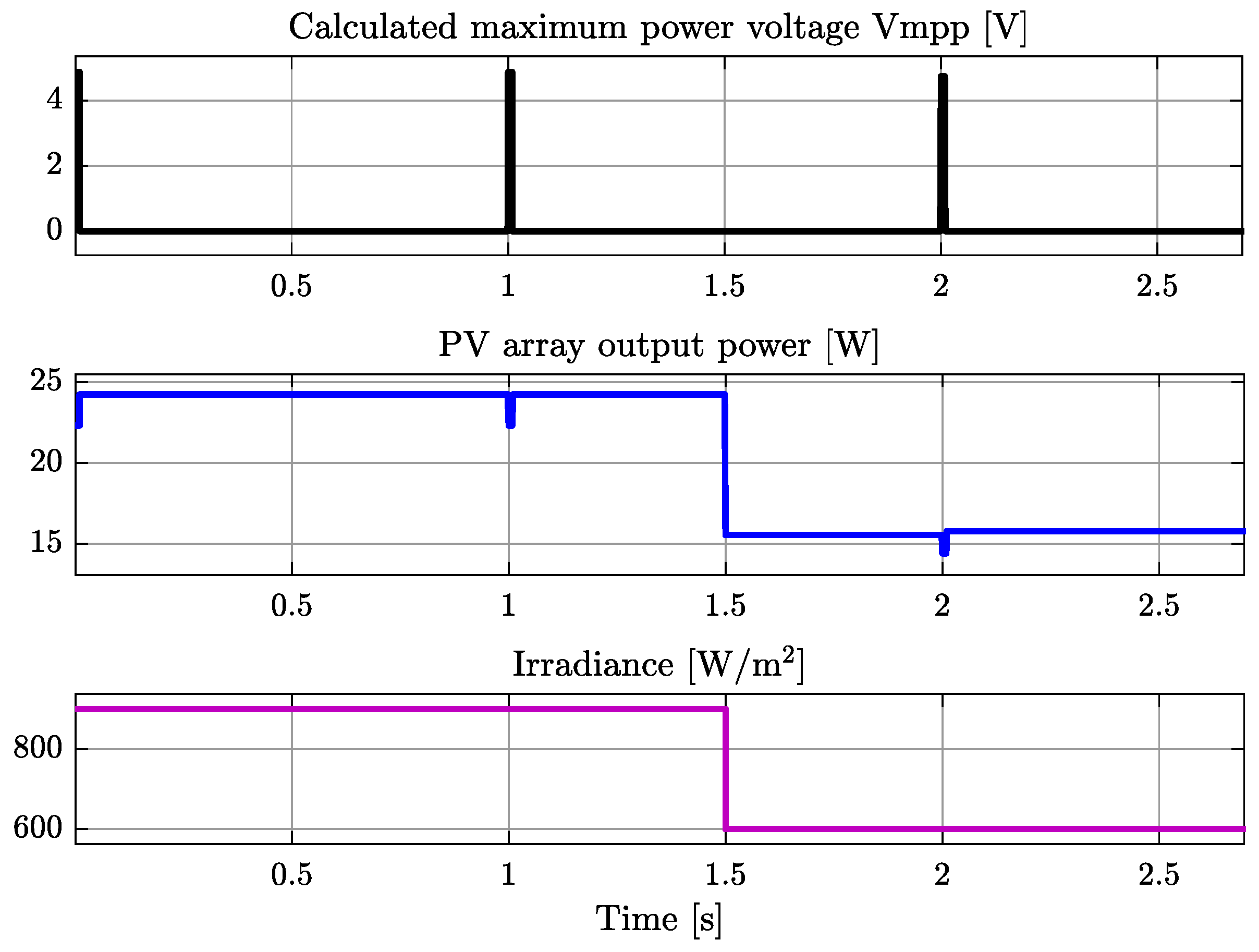
The third case presents the sudden drop in the irradiance from 900 to 600 W/m², as shown in Figure 12. In this example, the first two measuring periods corresponding to 0–0.01 s and 1–1.01 s are performed under the same irradiance of 900 W/m². Therefore, the same open circuit voltage of 0.596 V is measured on the semi-pilot. During these measuring periods, the DC-DC converter is set to the $V_{mpp}=4.37$ V. After these measurement periods begin supply periods that take place between 0.01–1 s and 1.01–2 s. The corresponding DC-DC converter’s voltage is calculated by $V_{mpp}=4.86$ V. Although there is change of irradiance in the middle of the second supply period (at 1.5 s) from 900 to 600 W/m², the DC-DC converter will stay tuned to the 4.86 V voltage which is not the maximal power voltage for the irradiance of 600 W/m². As a result, the output power of the PV array will be 15.7 W instead of maximal 15.78 W. The difference between the maximal and obtained powers is only 0.08 W (0.5%) because $V_{mpp}$ voltage is almost uninfluenced by the irradiance variations unlike the $I_{mpp}$ current which is significantly effected by the irradiance changes, see Figure 8. This small mismatch can be further reduced by increasing the frequency of the operation cycle according to the irradiance conditions. During the third measurement period (2–2.01 s), the measured open circuit voltage of the semi-pilot is 0.58 V that corresponds to the $V_{mpp}=4.26$ V. After the third measurement period, in the following supply periods, the DC-DC converter is operated with $V_{mpp}=4.73$ V which is updated to the irradiance of 600 W/m² and the output power of the PV array is increased to 15.78 W. These simulations show that the proposed SPC-FOCV method is accurate for constant and varying irradiance conditions.

The first scenario was extended and simulated for constant irradiance values of 800, 600, 400, and 200 W/m². The $V_{mpp}$ voltages calculated by SPC-FOCV method can be compared to the $V_{mpp}$ voltages measured from the graph shown in Figure 9. This comparison is presented in

Table 4. Comparison between measured and estimated $V_{mpp}$ voltages for different irradiance values.

Irradiance [W/m2]	1000	800	600	400	200
$V_{mpp}$ (measured) [V]	4.896	4.825	4.736	4.608	4.39
$V_{mpp}$ (estimated by SPC-FOCV) [V]	4.896	4.825	4.736	4.608	4.38
Error [%]	0	0	0	0	0.2

which shows that there is an accurate match between the measured and estimated $V_{mpp}$ until irradiance values of 200 W/m², where the estimation error rises from zero to 0.2%.

The proposed SPC-FOCV method is compared to the conventional FOCV, pilot cell-based FOCV and P&O methods in

Table 5. Comparison between the proposed SPC-FOCV, conventional FOCV, and the pilot cell-based FOCV methods.

Irradiance [W/m2]	1000				600				200
Method	Pmax	Psup	ΔPtot	η	Pmax	Psup	ΔPtot	η	Pmax	Psup	ΔPtot	η
SPC ($D_c$ = 99%)	27.14	27.11	0.22	99.07	15.78	15.76	0.09	99.3	4.84	4.83	0.018	99.42
SPC ($D_c$ = 95%)	27.14	27	0.33	98.26	15.78	15.7	0.15	98.54	4.84	4.81	0.038	98.59
SPC ($D_c$ = 90%)	27.14	26.86	0.47	97.23	15.78	15.62	0.23	97.52	4.84	4.79	0.085	97.21
Pilot Cell	27.14	24.42	2.71	90	15.78	14.2	1.57	90	4.84	4.35	0.48	90
FOCV ($D_c$ = 99%)	27.14	26.86	0.45	97.31	15.78	15.62	0.21	97.65	4.84	4.79	0.048	97.97
FOCV ($D_c$ = 95%)	27.14	25.78	1.53	89.35	15.78	14.99	0.84	89.67	4.84	4.59	0.247	89.73
FOCV ($D_c$ = 90%)	27.14	24.42	2.88	79.36	15.78	14.2	1.63	79.65	4.84	4.35	0.437	80.84
P&O	27.14	27.14	0	100	15.78	15.78	0	100	4.84	4.84	0	100

, for different irradiance levels and duty cycles $D_c$ at constant cells temperature of 25 °C, which is the nominal temperature of the cells. The comparison is based on PV supplied power $P_{\sup }$, total power losses $\Delta P_{tot}$, and the efficiency $\eta$.

The SPC-FOCV calculated power losses for different irradiance values are shown in

Table 6. Calculated switches power losses for different irradiance values, SPC-FOCV. Switching frequency is 1 Hz.

Irradiance [W/m2]	1000	600	200
Conduction power losses [W]	0.19	0.07	8.15m
Switching power losses [W]	0.29u	0.17u	0.051u
Total power losses $\Delta P_{sw}$ [W]	0.19	0.07	8.15m

. It can be seen that the sum of the calculated switching losses of switches 1 and bypass has very low values- [uW] and therefore, only the the conduction losses effect the total power losses of the Mosfets. If the switching frequency will be significantly increased to the values of kHz, the switching losses will become more dominant and they will have to be taken into account.

Table 5 shows that for all simulated values of irradiance and duty cycles, the proposed SPC-FOCV method ensures highest supplied power $P_{\sup }$, lowest power losses $P_{loss}$ and as a result highest efficiency compared to the conventional FOCV and the pilot cell methods.

The increase of the duty cycle results in higher efficiency. Therefore, the duty cycle should be set to the highest possible value. The operation frequency should be defined according to two parameters- estimation accuracy and switching power losses. The increase of the operation frequency will result in better accuracy of the estimated $V_{MPP}$ voltage but the Mosfet power losses will be also increased and the efficiency will be decreased. Therefore, the operation frequency should be matched according to the irradiance conditions of the PV installation.

The P&O method identifies the maximum power point without disconnection of the PV from the load and therefore, the power losses are zero and its efficiency is 100%. However, the implementation of the P&O method is more complicated and requires DSP.

4.2. SPC-FOCV Operation under Temperature Variations

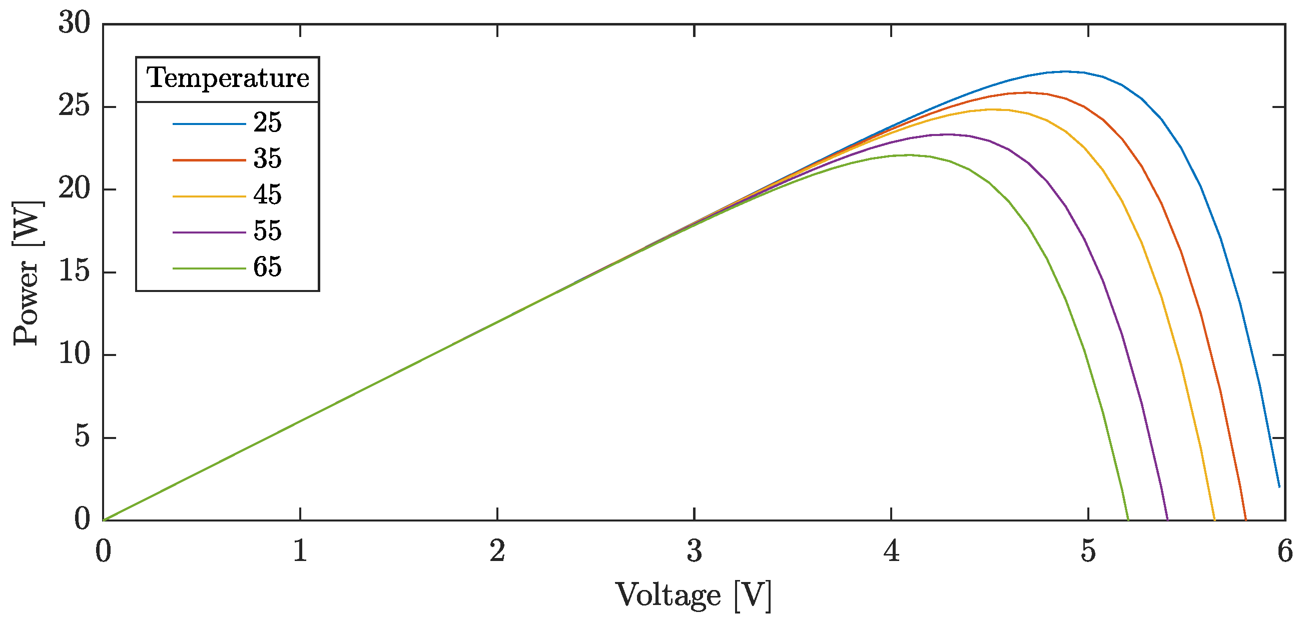
Other set of simulations was performed for temperature variations between 25 °C to 65 °C while the irradiance was kept constant at 1000 W/m² (the nominal temperature of the simulated panel is 25 °C). The graph of the simulated PV output power vs. output voltage curves for different temperature values is shown in Figure 13. This graph can be used in order to measure the value of the PV array’s $V_{mpp}$ voltage for each specific temperature. These curves were obtained by using simulation setup shown in Figure 9 where the temperature of the PV array was changed according to the desired curve. It can be seen that the temperature variations significantly effect the open-circuit voltage which is reduced when the temperature is increased. The calculated voltage factor for different temperature values is shown in

Table 7. The calculated voltage factor for different temperature values.

Temperature	25	35	45	55	65
$K_{pv}$ (calculated)	0.816	0.816	0.801	0.795	0.789

.

Table 7 shows that the voltage factor decreases when temperature changes from 45 °C to 65 °C. Therefore, for these temperature values an error in $V_{mpp}$ estimation is expected.

The PV panel from the previous section was operated by SPC-FOCV at 25 to 35, 45, 55, and 65 °C with operation cycle of 1 s and $D_c$ = 99%. The $V_{mpp}$ voltages calculated by SPC-FOCV method under varying temperatures can be compared to the $V_{mpp}$ voltages measured from the graph shown in Figure 13. This comparison is presented in

Table 8. Comparison between directly measured and SPC-FOCV estimated $V_{mpp}$ voltage for different temperature values.

Temperature	25	35	45	55	65
$V_{mpp}$ (measured) [V]	4.896	4.735	4.49	4.3	4.11
$V_{mpp}$ (estimated by SPC-FOCV) [V]	4.896	4.735	4.573	4.411	4.249
Error [%]	0	0	0.28	0.51	0.95

. It can be seen that $V_{mpp}$ estimation error appears at temperature of 45 °C and increases with the temperature rise. At temperature of 65 °C, the estimation error is maximal 0.95%. However, this error value is very low and acceptable according to IEEE standards.

It can be seen that the SPC-FOCV method provides precise estimation of $V_{mpp}$ voltage during the irradiance and temperature changes except for high temperature and/or low irradiance values where small errors are present. Additional errors can appear if the irradiance or temperature vary very fast while the frequency of the operation cycle is too low and not matched to the rate of changes in irradiance or temperature. This inaccuracy can be reduced or completely avoided by increasing the frequency of the operation cycle according to the irradiance or temperature conditions.

The semi-pilot cell and its switching mechanism has to be integrated into the PV array during its manufacturing process. The proposed SPC-FOCV method is more suitable for small PV systems consisted of limited number of PV panels. The integration of the semi-pilot cell in every panel of a large PV system with many PV panels would require high manufacturing costs.

5. Semi-Pilot Panel SPP-FOCV Method

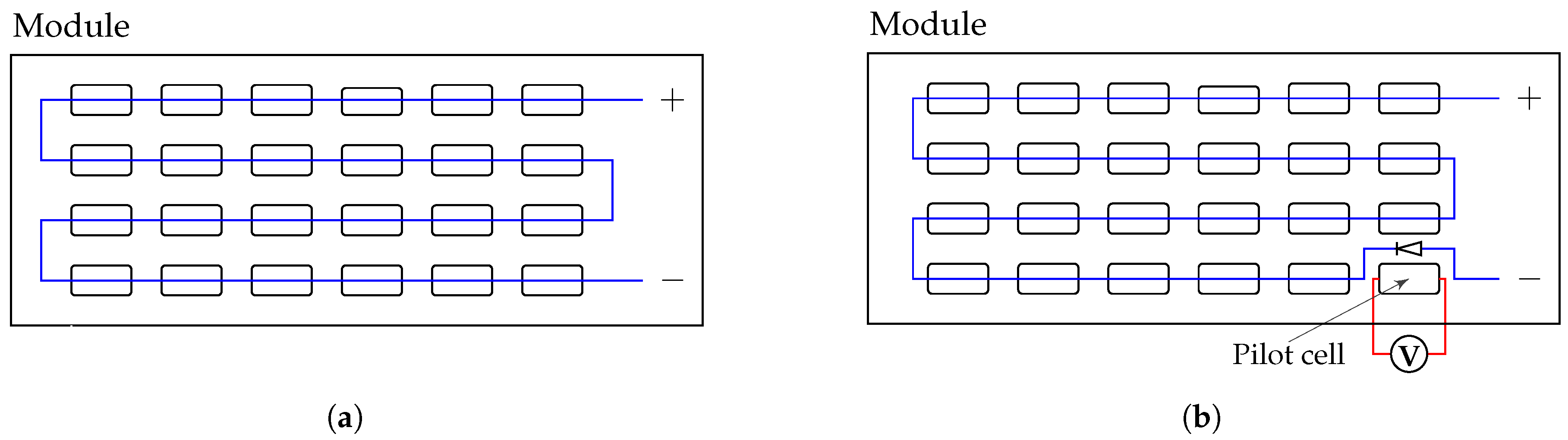
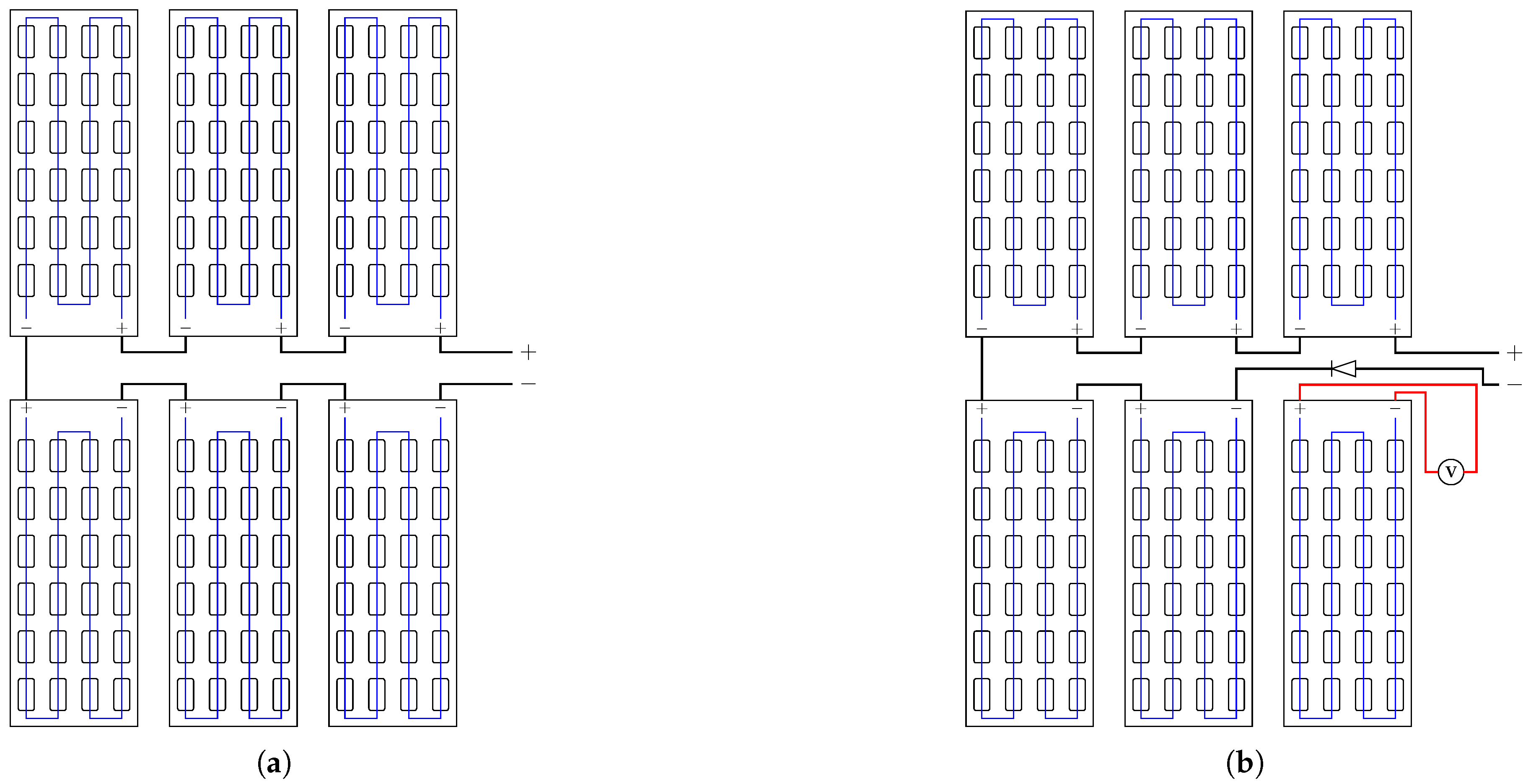
The SPP-FOCV method is intended for application in large PV systems consisted of many PV panels, see Figure 14. The semi-pilot panel method is the extended version of the semi-pilot cell method and their operation principle is similar. The $V_{mpp}$ voltage of the whole PV system is estimated by measuring the open circuit voltage of the semi-pilot panel. The operation cycle is divide into two stages- during the first stage the semi-pilot panel feeds the load and during the second stage, the semi-pilot panel is switched off from the array by two transistors and bypassed by the diode. During the measurement only $N-1$ panels supply power to the load. Unlike the SPC-FOCV where semi-pilot cell and its switching circuit have to be internally integrated into the PV array during PV manufacturing, the semi-pilot panel and the switching circuit in the SPP-FOCV method are external and can be installed during the deployment of the PV system. Equations (2)–(9), which were presented earlier for SPC-FOCV method, are also valid for the SPP-FOCV method.

6. Experimental Validation and Analysis of the SPP-FOCV Method

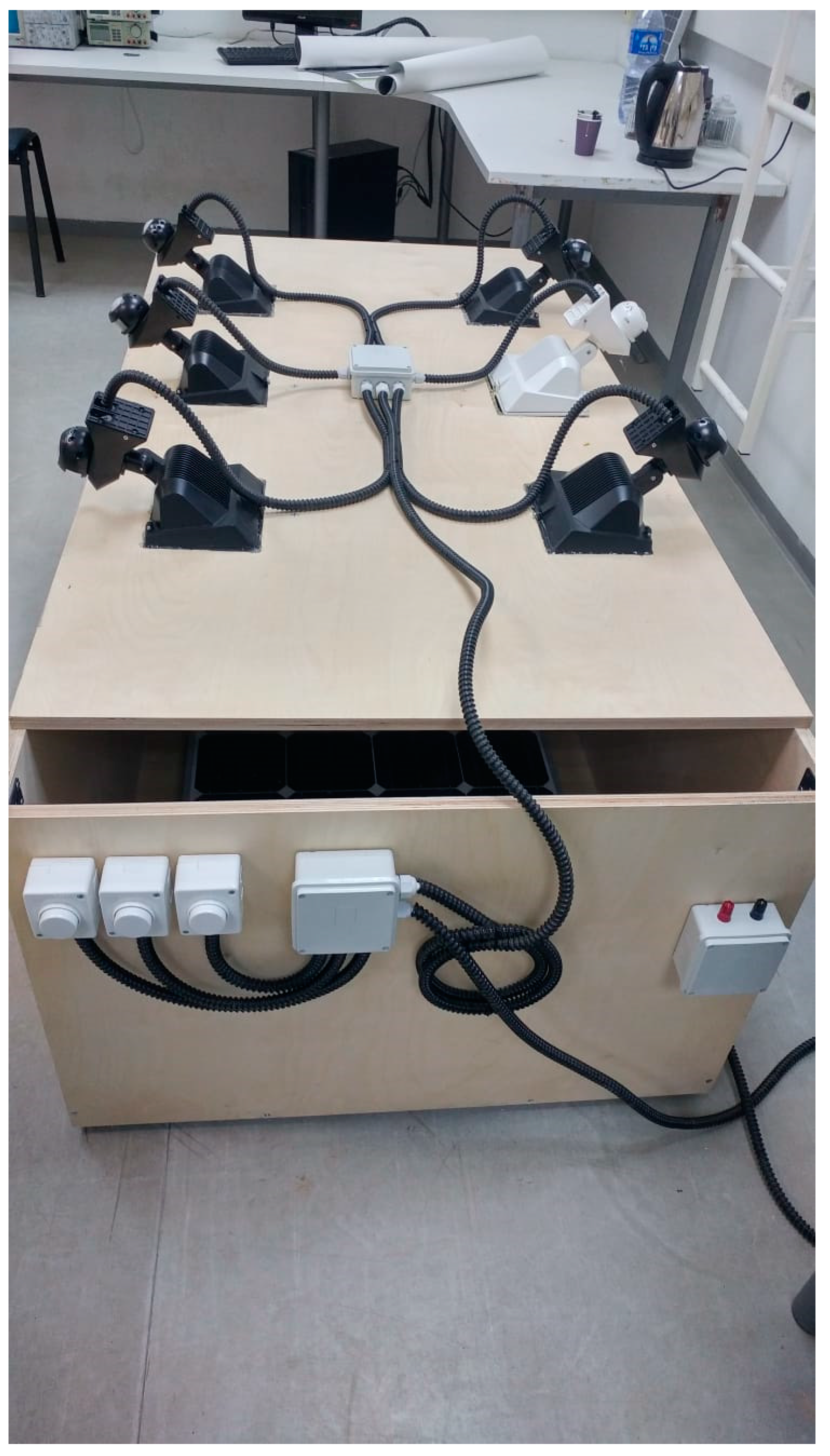
To experimentally verify the operation of the proposed SPP-FOCV method, a special box was constructed, see Figure 15. The purpose of this box is to set the desired irradiance values for each PV panel and to eliminate the effect of light from outside. Six 500 W lamps were installed on the top of the box. Each pair of lamps is installed above PV panel and equipped with dimmer that allows precise irradiance control. For each experiment, the lamps were tuned to the specific irradiance values that were applied to the PV panels.

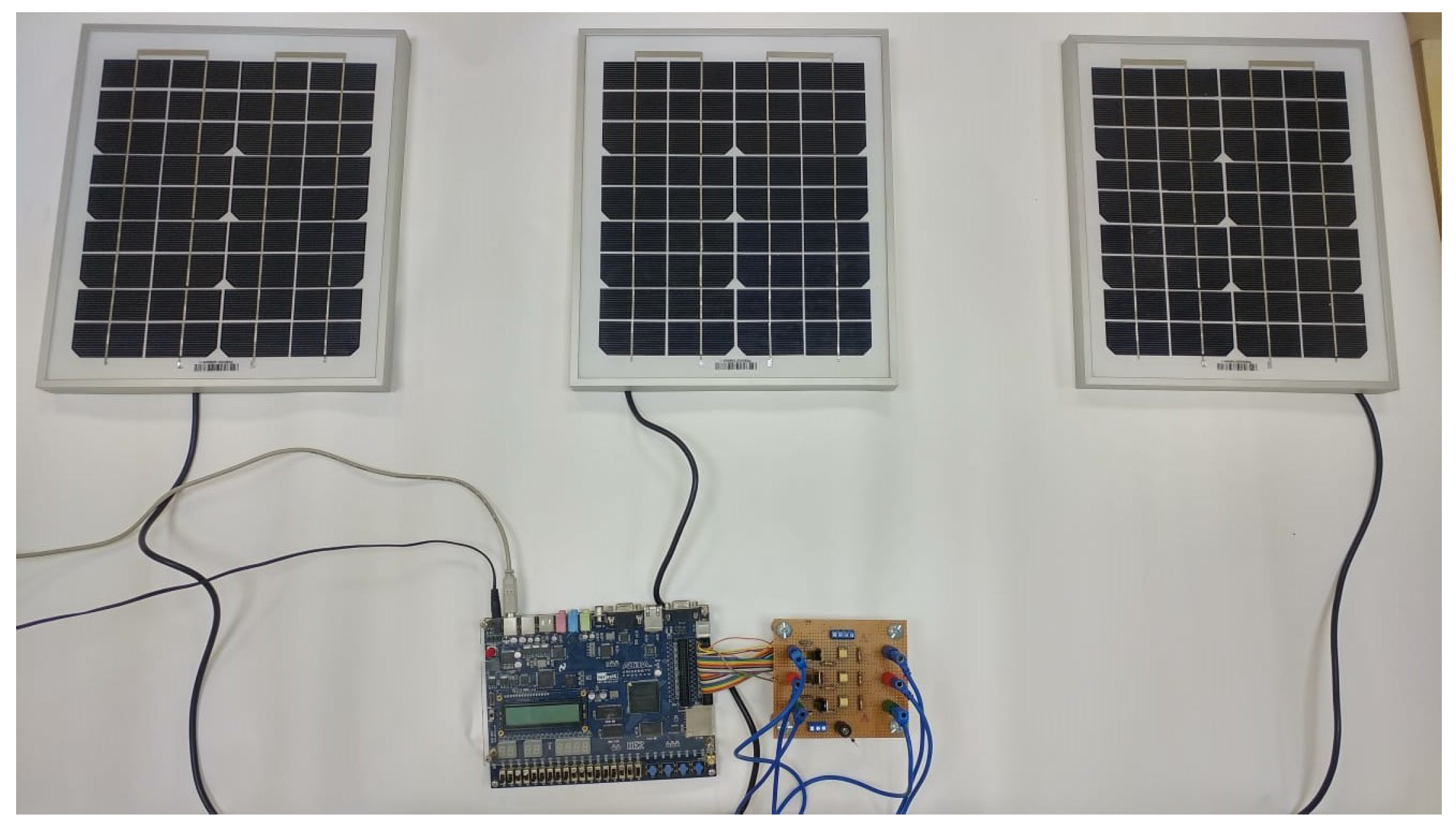
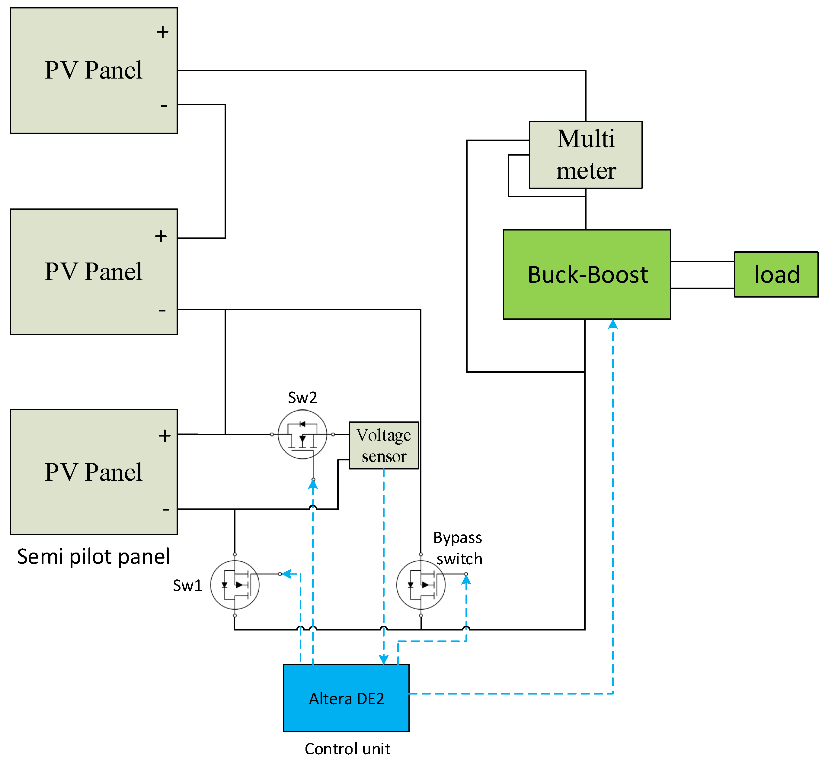
The three tested PS10M-12/B PV panels are connected in series and installed inside the box, under the lamps, as shown in Figure 16. The principle scheme of the experimental setup is shown in Figure 17. It is operated in the same manner as explained in Section 3. Each panel consists of 36 mono-crystal Si solar cells connected in series. The parameters of the panels are shown in

Table 9. Technical parameters of PS10M-12/B PV module.

Parameter	Value
Rated power [W]	10
Open circuit voltage [V]	21.4
Short circuit current [A]	0.68
Rated voltage [V]	16.8
Rated current [A]	0.6
Nominal operation temperature [°C]	45

. The calculated voltage factor of these PV panels is 0.8. The third panel is the semi-pilot panel equipped with three Mosfet switches (switches 1, 2 and bypass). The control unit for switches and Buck-Boost converter control is implemented by Altera DE2. The switches are implemented by CSD19531KCS Mosfets. The open circuit voltage of the semi-pilot panel is measured by the voltage sensor and its value is transfered to the Altera. The accuracy of the voltage sensor used in the experimental setup is ±5 mV. The PV array’s output power is measured by the GPM-8212 multi-meter whose accuracy is ±0.2% of reading.

Two sets of experiments were performed in order to verify the proposed FOCV-SPP method. The complete operation cycle of the semi-pilot panel was set 1 s (frequency 1 Hz) with duty cycle of 99% i.e., the semi-pilot panel feeds the load during 0.99 s together with other two panels and disconnected for open circuit voltage measurement for 0.01 s. The $V_{mpp}$ voltage was estimated by multiplying the measured open circuit voltage of the switched semi-pilot panel by voltage factor $K_{pv}$ and the number of solar modules in the PV array (three). The estimated $V_{mpp}$ voltage was compared to the directly measured $V_{mpp}$ voltage that was obtained before testing the FOCV-SPP method. To obtain the directly measured $V_{mpp}$ voltage, three PV panels were tested for each irradiance value under load implemented by varying voltage source that was swept between zero to $V_{oc}=64.2$ V voltage of the array.

During the first set of experiments, the $V_{mpp}$ voltage was estimated by the FOCV-SPP method for different irradiance values while the ambient and PV cells temperature was 25 °C. The comparison between directly measured and FOCV-SPP calculated $V_{mpp}$ voltage for this set of experiments is shown in

Table 10. Experimental comparison between directly measured and SPP-FOCV estimated $V_{mpp}$ voltage for different irradiance values. The temperature of the PV cells is 25 °C.

Irradiance [W/m2]	1000	800	600	400	200
Output power [W]	30.3	23.73	17.1	10.7	4.9
Directly measured $V_{mpp}$ voltage [V]	50.2	49	47.3	45.5	43
SPP-FOCV estimated $V_{mpp}$ voltage [V]	50.1	48.9	47.1	44.9	42.4
Measured $V_{oc}$ of semi-pilot panel [V]	20.87	20.37	19.6	18.7	18
Estimation error [%]	0.1	0.2	0.4	1.3	1.4

.

It can be seen that estimation of the $V_{mpp}$ voltage by the proposed SPP-FOCV algorithm is precise under various irradiance conditions. The maximal estimation error is around 1.4%.

The second set of experiments was performed under partial shading conditions. In general, the standard FOCV method is not intended for use under partial shading conditions, as well as many other common MPPT methods such as P&O, IC etc. The accuracy of these methods is limited under partial shading conditions. Therefore, the proposed SPP-FOCV method which is improvement of the standard FOCV method, is also is not intended for implementation under partial shading conditions. A lot of special MPPT methods for partial shading conditions were developed and presented in the literature [56,57,58].

To understand how the accuracy of the proposed SPP-FOCV method will be effected under partial shading conditions, the experimental setup was tested under three partial shading cases while the temperature of the cells was 25 °C. In the first case, the irradiance of 400 W/m² was applied to the PV panel 1, 600 W/m² to the PV panel 2 and 800 W/m² to the PV panel 3 (semi-pilot panel). In the second case, the irradiance of 800 W/m² was applied to the PV panel 1, 600 W/m² to the PV panel 2 and 400 W/m² to the PV panel 3 (semi-pilot panel). In the third case, the irradiance of 800 W/m² was applied to the PV panel 1, 400 W/m² to the PV panel 2 and 600 W/m² to the PV panel 3 (semi-pilot panel). The obtained experimental results are shown in

Table 11. Experimental comparison between directly measured and SPP-FOCV estimated $V_{mpp}$ voltage under partial shading conditions. The temperature of the PV cells is 25 °C.

Case	1	2	3
Irradiance on PV panel 1 [W/m2]	400	800	800
Irradiance on PV panel 2 [W/m2]	600	600	400
Irradiance on PV panel 3 (semi-pilot panel) [W/m2]	800	400	600
Directly measured $V_{mpp}$ voltage [V]	50.8	50.8	50.8
SPP-FOCV estimated $V_{mpp}$ voltage [V]	48.9	44.9	47.1
Measured $V_{oc}$ of semi-pilot panel [V]	20.37	18.7	19.6
Estimation error [%]	3.8	13.1	7.8

.

This Table shows that the lowest estimation error of 3.8% was obtained in case 1 where the irradiance on the semi-pilot panel was highest (800 W/m²) while the largest error (13.1%) was obtained in case 2 where the irradiance on the semi-pilot panel was lowest (400 W/m²). Therefore, in some cases of the partial shading, the proposed SPP-FOCV method will be accurate enough while in other cases, its accuracy will be limited and the special partial shading MPPT methods should be used.

7. Conclusions

Two general challenges of the conventional FOCV method are to improve the accuracy and to reduce the power loss. To solve these issues, we propose to reduce the power loss during open-circuit voltage measurements by replacing the pilot cell by a semi-pilot cell. During normal operation, the semi-pilot cell is a part of the PV array and contributes to the total generated power. The open-circuit voltage is measured when the semi-pilot cell is disconnected from the array. As a result the power of the semi-pilot cell is lost only when it is disconnected, and not constantly. The proposed methods are validated using simulations and experiments. It is shown that both methods can accurately estimate the maximum power point voltage, and hence improve the overall efficiency.

References

- Barchowsky, A.; Parvin, J.P.; Reed, G.F.; Korytowski, M.J.; Grainger, B.M. A comparative study of MPPT methods for distributed photovoltaic generation. In Proceedings of the IEEE PES Innovative Smart Grid Technologies, Washington, DC, USA, 16–18 January 2012; pp. 1–7. [Google Scholar]
- De Brito, M.A.G.; Galotto, L.; Sampaio, L.P.; de Azevedo e Melo, G.; Canesin, C.A. Evaluation of the main MPPT techniques for photovoltaic applications. IEEE Trans. Ind. Electron. 2013, 60, 1156–1167. [Google Scholar] [CrossRef]
- Esram, T.; Chapman, P.L. Comparison of photovoltaic array maximum power point tracking techniques. IEEE Trans. Energy Convers. 2007, 22, 439–449. [Google Scholar] [CrossRef]
- Murtaza, A.F.; Sher, H.A.; Chiaberge, M.; Boero, D.; Giuseppe, M.D.; Addoweesh, K.E. Comparative analysis of maximum power point tracking techniques for PV applications. In Proceedings of the 16th International Multi Topic Conference, Lahore, Pakistan, 19–20 December 2013; pp. 83–88. [Google Scholar]
- Subudhi, B.; Pradhan, R. A comparative study on maximum power point tracking techniques for photovoltaic power systems. IEEE Trans. Sustain. Energy 2013, 4, 89–98. [Google Scholar] [CrossRef]
- Bastidas-Rodriguez, J.D.; Franco, E.; Petrone, G.; Ramos-Paja, C.A.; Spagnuolo, G. Maximum power point tracking architectures for photovoltaic systems in mismatching conditions: A review. IET Power Electron. 2014, 7, 1396–1413. [Google Scholar] [CrossRef]
- Elobaid, L.M.; Abdelsalam, A.K.; Zakzouk, E.E. Artificial neural network-based photovoltaic maximum power point tracking techniques: A survey. IET Renew. Power Gener. 2015, 9, 1043–1063. [Google Scholar] [CrossRef]
- Bendib, B.; Belmili, H.; Krim, F. A survey of the most used MPPT methods: Conventional and advanced algorithms applied for photovoltaic systems. Renew. Sustain. Energy Rev. 2015, 45, 637–648. [Google Scholar] [CrossRef]
- Dolara, A.; Faranda, R.; Leva, S. Energy comparison of seven MPPT techniques for PV systems. J. Electromagn. Anal. Appl. 2009, 1, 152. [Google Scholar] [CrossRef]
- Hsieh, G.C.; Hsieh, H.I.; Tsai, C.Y.; Wang, C.H. Photovoltaic power-increment-aided incremental-conductance MPPT with two-phased tracking. IEEE Trans. Power Electron. 2013, 28, 2895–2911. [Google Scholar] [CrossRef]
- Safari, A.; Mekhilef, S. Simulation and hardware implementation of incremental conductance MPPT with direct control method using Cuk converter. IEEE Trans. Ind. Electron. 2011, 58, 1154–1161. [Google Scholar] [CrossRef]
- Hossain, M.J.; Tiwari, B.; Bhattacharya, I. An adaptive step size incremental conductance method for faster maximum power point tracking. In Proceedings of the 2016 IEEE 43rd Photovoltaic Specialists Conference, Portland, OR, USA, 5–10 June 2016; pp. 3230–3233. [Google Scholar]
- Lakshmi, D.; Rashmi, M. A modified incremental conductance algorithm for partially shaded PV array. In Proceedings of the 2017 International Conference on Technological Advancements in Power and Energy, Kollam, India, 21–23 Decembner 2017; pp. 1–6. [Google Scholar]
- Tey, K.S.; Mekhilef, S. Modified incremental conductance MPPT algorithm to mitigate inaccurate responses under fast-changing solar irradiation level. Sol. Energy 2014, 101, 333–342. [Google Scholar] [CrossRef]
- Lokanadham, M.; Bhaskar, K.V. Incremental conductance based maximum power point tracking (MPPT) for photovoltaic system. Int. J. Eng. Res. Appl. 2012, 2, 1420–1424. [Google Scholar]
- Sivakumar, P.; Kader, A.A.; Kaliavaradhan, Y.; Arutchelvi, M. Analysis and enhancement of PV efficiency with incremental conductance MPPT technique under non-linear loading conditions. Renew. Energy 2015, 81, 543–550. [Google Scholar] [CrossRef]
- Kish, G.J.; Lee, J.J.; Lehn, P. Modelling and control of photovoltaic panels utilising the incremental conductance method for maximum power point tracking. IET Renew. Power Gener. 2012, 6, 259–266. [Google Scholar] [CrossRef]
- Dhar, S.; Sridhar, R.; Mathew, G. Implementation of PV cell based standalone solar power system employing incremental conductance MPPT algorithm. In Proceedings of the 2013 International Conference on Circuits, Power and Computing Technologies, Nagercoil, India, 20–21 March 2013; pp. 356–361. [Google Scholar]
- Xiong, Y.; Qian, S.; Xu, J. Research on constant voltage with incremental conductance MPPT method. In Proceedings of the Power and Energy Engineering Conference, 2012 Asia-Pacific, Shanghai, China, 27–29 March 2012; pp. 1–4. [Google Scholar]
- Zhu, W.; Shang, L.; Li, P.; Guo, H. Modified hill climbing MPPT algorithm with reduced steady-state oscillation and improved tracking efficiency. J. Eng. 2018, 2018, 1878–1883. [Google Scholar] [CrossRef]
- Al-Atrash, H.; Batarseh, I.; Rustom, K. Effect of measurement noise and bias on hill-climbing MPPT algorithms. IEEE Trans. Aerosp. Electron. Syst. 2010, 46, 745–760. [Google Scholar] [CrossRef]
- Kjær, S.B. Evaluation of the “Hill climbing” and the “Incremental conductance” maximum power point trackers for photovoltaic power systems. IEEE Trans. Energy Convers. 2012, 27, 922–929. [Google Scholar] [CrossRef]
- Xiao, W.; Dunford, W.G. A modified adaptive hill climbing MPPT method for photovoltaic power systems. In Proceedings of the 2004 IEEE 35th Annual Power Electronics Specialists Conference, Aachen, Germany, 20–25 June 2004; pp. 1957–1963. [Google Scholar]
- Al-Atrash, H.; Batarseh, I.; Rustom, K. Statistical modeling of DSP-based hill-climbing MPPT algorithms in noisy environments. In Proceedings of the Twentieth Annual IEEE Applied Power Electronics Conference, Austin, TX, USA, 6–10 March 2005; pp. 1773–1777. [Google Scholar]
- Peftitsis, D.; Adamidis, G.; Balouktsis, A. A new MPPT method for Photovoltaic generation systems based on Hill Climbing algorithm. In Proceedings of the 2008 International Conference on Electrical Machines, Wuhan, China, 17–20 October 2008. [Google Scholar]
- Abuzed, S.; Foster, M.; Stone, D. Variable PWM step-size for modified Hill climbing MPPT PV converter. In Proceedings of the 7th IET International Conference on Power Electronics, Machines and Drives (PEMD 2014), Manchester, UK, 8–10 April 2014. [Google Scholar]
- Ahmed, A.; Ran, L.; Bumby, J. Perturbation parameters design for hill climbing MPPT techniques. In Proceedings of the 2012 IEEE International Symposium on Industrial Electronics, Hangzhou, China, 28–31 May 2012; pp. 1819–1824. [Google Scholar]
- Elgendy, M.; Zahawi, B.; Atkinson, D. Dynamic behaviour of hill-climbing MPPT algorithms at low perturbation rates. In Proceedings of the IET Conference on Renewable Power Generation, Edinburgh, UK, 6–8 September 2011. [Google Scholar]
- Raza, K.S.M.; Goto, H.; Guo, H.J.; Ichinokura, O. A novel speed-sensorless adaptive hill climbing algorithm for fast and efficient maximum power point tracking of wind energy conversion systems. In Proceedings of the IEEE International Conference on Sustainable Energy Technologies, Singapore, 24–27 November 2008; pp. 628–633. [Google Scholar]
- Bahari, M.I.; Tarassodi, P.; Naeini, Y.M.; Khalilabad, A.K.; Shirazi, P. Modeling and simulation of hill climbing MPPT algorithm for photovoltaic application. In Proceedings of the 2016 International Symposium on Power Electronics, Electrical Drives, Automation and Motion, Anacapri, Italy, 22–24 June 2016; pp. 1041–1044. [Google Scholar]
- Elgendy, M.A.; Zahawi, B.; Atkinson, D.J. Assessment of perturb and observe MPPT algorithm implementation techniques for PV pumping applications. IEEE Trans. Sustain. Energy 2012, 3, 21–33. [Google Scholar] [CrossRef]
- Raj, C.M.J.S.; Jeyakumar, A.E. A novel maximum power point tracking technique for photovoltaic module based on power plane analysis of I–V characteristics. IEEE Trans. Ind. Electron. 2014, 61, 4734–4745. [Google Scholar] [CrossRef]
- Sera, G.; Teodorescu, R.; Hantschel, J.; Knoll, M. Optimized maximum power point tracker for fast-changing environmental conditions. IEEE Trans. Ind. Electron. 2008, 55, 2629–2637. [Google Scholar] [CrossRef]
- Femia, N.; Petrone, G.; Spagnuolo, G.; Vitelli, M. A technique for improving P&O MPPT performances of double-stage grid-connected photovoltaic systems. IEEE Trans. Ind. Electron. 2009, 56, 4473–4482. [Google Scholar]
- Femia, N.; Petrone, G.; Spagnuolo, G.; Vitelli, M. Optimizing duty-cycle perturbation of P&O MPPT technique. In Proceedings of the 2004 IEEE 35th Annual Power Electronics Specialists Conference, Aachen, Germany, 20–25 June 2004; pp. 1939–1944. [Google Scholar]
- Al-Diab, A.; Sourkounis, C. Variable step size P&O MPPT algorithm for PV systems. In Proceedings of the 12th International Conference on Optimization of Electrical and Electronic Equipment, Brasov, Romania, 20–22 May 2010; pp. 1097–1102. [Google Scholar]
- Kollimalla, S.K.; Mishra, M.K. A novel adaptive P&O MPPT algorithm considering sudden changes in the irradiance. IEEE Trans. Energy Convers. 2014, 29, 602–610. [Google Scholar]
- Sher, H.A.; Murtaza, A.F.; Noman, A.; Addoweesh, K.E.; Al-Haddad, K.; Chiaberge, M. A new sensorless hybrid MPPT algorithm based on fractional short-circuit current measurement and P&O MPPT. IEEE Trans. Sustain. Energy 2015, 6, 1426–1434. [Google Scholar]
- Al Nabulsi, A.; Dhaouadi, R. Efficiency optimization of a DSP-based standalone PV system using fuzzy logic and dual-MPPT control. IEEE Trans. Ind. Inf. 2012, 8, 573–584. [Google Scholar] [CrossRef]
- Chikh, A.; Chandra, A. An optimal maximum power point tracking algorithm for PV systems with climatic parameters estimation. IEEE Trans. Sustain. Energy 2015, 6, 644–652. [Google Scholar] [CrossRef]
- Chiu, C.S.; Ouyang, Y.L. Robust maximum power tracking control of uncertain photovoltaic systems: A unified TS fuzzy model-based approach. IEEE Trans. Control Syst. Technol. 2011, 19, 1516–1526. [Google Scholar] [CrossRef]
- Larbes, C.; Aït Cheikh, S.M.; Obeidi, T.; Zerguerras, A. Genetic algorithms optimized fuzzy logic control for the maximum power point tracking in photovoltaic system. Renew. Energ. 2009, 34, 2093–2100. [Google Scholar] [CrossRef]
- Vinay, P.; Mathews, M.A. Modelling and analysis of artificial intelligence based MPPT techniques for PV applications. In Proceedings of the 2014 International Conference on Advances in Green Energy, Thiruvananthapuram, India, 17–18 December 2014; pp. 56–65. [Google Scholar]
- Ahmad, J. A fractional open circuit voltage based maximum power point tracker for photovoltaic arrays. In Proceedings of the 2nd International Conference on Software Technology and Engineering, San Juan, PR, USA, 3–5 October 2010; Volume 1, pp. V1-247–V1-250. [Google Scholar]
- Sandali, A.; Oukhoya, T.; Cheriti, A. Modeling and design of PV grid connected system using a modified fractional short-circuit current MPPT. In Proceedings of the 2014 International Renewable and Sustainable Energy Conference, Ouazazate, Morocco, 17–19 October 2014; pp. 224–229. [Google Scholar]
- Khatib, T.T.; Mohamed, A.; Amim, N.; Sopian, K. An improved indirect maximum power point tracking method for standalone photovoltaic systems. In Proceedings of the 9th WSEAS International Conference on Applications of Electrical Engineering, Selangor, Malaysia, 23–25 March 2010; pp. 56–62. [Google Scholar]
- Vitorino, M.A.; Hartmann, L.V.; Lima, A.M.; Correa, M.B. Using the model of the solar cell for determining the maximum power point of photovoltaic systems. In Proceedings of the 2007 European Conference on Power Electronics and Applications, Aalborg, Denmark, 2–5 September 2007; pp. 1–10. [Google Scholar]
- Chang, S.; Wang, Q.; Hu, H.; Ding, Z.; Guo, H. An NNwC MPPT-based energy supply solution for sensor nodes in buildings and its feasibility study. Energies 2019, 12, 101. [Google Scholar] [CrossRef]
- Harrag, A.; Messalti, S. Variable step size modified P&O MPPT algorithm using GA-based hybrid offline/online PID controller. Renew. Sustain. Energy Rev. 2015, 49, 1247–1260. [Google Scholar]
- Li, W.; He, X. Review of nonisolated high-step-up DC/DC converters in photovoltaic grid-connected applications. IEEE Trans. Ind. Electron. 2011, 58, 1239–1250. [Google Scholar] [CrossRef]
- York, B.; Yu, W.; Lai, J.S. An integrated boost resonant converter for photovoltaic applications. IEEE Trans. Power Electron. 2013, 28, 1199–1207. [Google Scholar] [CrossRef]
- Baimel, D.; Shkoury, R.; Elbaz, L.; Tapuchi, S.; Baimel, N. Novel optimized method for maximum power point tracking in PV systems using Fractional Open Circuit Voltage technique. In Proceedings of the 2016 International Symposium on Power Electronics, Electrical Drives, Automation and Motion, Anacapri, Italy, 22–24 June 2016; pp. 889–894. [Google Scholar]
- Frezzetti, A.; Manfredi, S.; Suardi, A. Adaptive FOCV-based control scheme to improve the MPP tracking performance: An experimental validation. IFAC Proc. Vol. 2014, 47, 4967–4971. [Google Scholar] [CrossRef]
- Huang, Y.P. A rapid maximum power measurement system for high-concentration photovoltaic modules using the fractional open-circuit voltage technique and controllable electronic load. IEEE J. Photovolt. 2014, 4, 1610–1617. [Google Scholar] [CrossRef]
- Lopez-Lapena, O.; Penella, M.T. Low-power FOCV MPPT controller with automatic adjustment of the sample & hold. Electron. Lett. 2012, 48, 1301–1303. [Google Scholar]
- Seyedmahmoudian, M.; Horan, B.; Soon, T.K.; Rahmani, R.; Oo, A.M.T.; Mekhilef, S.; Stojcevski, A. State of the art artificial intelligence-based MPPT techniques for mitigating partial shading effects on PV systems—A review. Renew. Sustain. Energy Rev. 2016, 64, 435–455. [Google Scholar] [CrossRef]
- Mohapatra, A.; Nayak, B.; Das, P.; Mohanty, K.B. A review on MPPT techniques of PV system under partial shading condition. Renew. Sustain. Energy Rev. 2017, 80, 854–867. [Google Scholar] [CrossRef]
- Lyden, S.; Haque, M.E.; Gargoom, A.; Negnevitsky, M. Review of maximum power point tracking approaches suitable for PV systems under partial shading conditions. In Proceedings of the 2013 Australasian Universities Power Engineering Conference, Hobart, Australia, 29 September–3 October 2013; pp. 1–6. [Google Scholar]
Figure 1.
The output voltage and current variations during irradiation and temperature changes. (a) PV module voltage-current graphs versus solar irradiance and temperature; (b) Maximum power point of a PV module.
Figure 2.
Pilot cell configuration.
Figure 3.
Semi-pilot cell disconnection during open-circuit voltage measurement.
Figure 4.
PV panel configuration during one measurement cycle. (a) First stage: all N cells provide power to the load, semi-pilot cell is connected to the array; (b) Second stage: semi-pilot cell is disconnected from the array.
Figure 5.
Operation cycle.
Figure 6.
Simulation setup of SPC-FOCV methods.
Figure 7.
Control unit.
Figure 8.
Output power with respect to output voltage during irradiance changes (100% irradiance corresponds to 1000 W/m2).
Figure 9.
Simulation setup for obtaining output power vs. output voltage curves. Temperature of the cells is 25 degrees.
Figure 10.
Scenario 1: Sunny day with constant irradiance.
Figure 11.
Scenario 2: Cloudy day with varying irradiance.
Figure 12.
Scenario 3: Sudden drop in the irradiance.
Figure 13.
Output power with respect to output voltage for various temperatures.
Figure 14.
PV array configuration during one measurement cycle. (a) First stage: all N panels provide power to the load, semi-pilot panel is connected to the array; (b) Second stage: the semi pilot panel is disconnected from the array.
Figure 15.
The box with six lamps and three dimmers that was designed for the experiments.
Figure 16.
The experimental setup with three PS10M-12/B PV modules connected in series, loads, and electronic control.
Figure 17.
The principle scheme of the experimental setup.