Impact of Co-Channel Interference on Two-Way Relaying Networks with Maximal Ratio Transmission


1
Department of Electronics and Communications Engineering, Yildiz Technical University, Esenler, 34220 Istanbul, Turkey
2
Computer Center, University of Mosul, Mosul 41002, Iraq
3
Department of Electrical and Electronics Engineering, Istanbul Medeniyet University, Uskudar, 34700 Istanbul, Turkey
*
Author to whom correspondence should be addressed.
Electronics 2019, 8(4), 392; https://doi.org/10.3390/electronics8040392
Submission received: 24 February 2019
/
Revised: 25 March 2019
/
Accepted: 27 March 2019
/
Published: 1 April 2019
(This article belongs to the Section Microwave and Wireless Communications)
Abstract
:Amplify-and-forward (AF) two-way relay networks (TWRNs) have become popular to provide spectrally efficient communication when range extension or energy efficiency is needed by utilizing a simple relay. However, their performance can be significantly degraded in practice due to co-channel interference (CCI) which is increasing due to growing number of wireless devices and recent cognitive and non-orthogonal multiple access techniques. With the motivation of improving the performance of AF-TWRNs, the use of maximal ratio transmission (MRT) is investigated to achieve high reliability while requiring low receiver complexity for the relay. First, the signal-to-interference-plus-noise ratio (SINR) expression is formulated and upper bounded. Then, tight lower bound expressions of outage probability (OP), sum symbol error rate (SSER), and upper bound ergodic sum rate (ESR) for each source and for the overall system are obtained. Besides, array and diversity gains are provided after deriving the asymptotic expressions of OP and SSER at high signal-to-noise ratio (SNR). Furthermore, the impact of channel estimation errors on the performance is also included. Finally, Monte Carlo simulation results which corroborate our theoretical findings are illustrated.
1. Introduction
Two-way relaying is a promising transmission technique to be used in next generation wireless networks where the relay can receive the sum of two source signals and then broadcast [1,2,3]. TWRNs allow the exchange of information within two time slots compared to four slots in dual hop relaying between two sources. Therefore, TWRNs can be useful in increasing the coverage or decreasing the transmit power in a spectrally efficient way. In order to have a low complexity relay for practical TWRNs, the amplify-and-forward (AF) approach is more preferable compared to other methods such as decode-and-forward (DF) which requires more processing [4]. Recently, TWRN technique has been applied to new communication scenarios. For example, Bastami et al. [5] considers the multiple-input multiple-output (MIMO) TWRN scheme with overlay cognitive radio (CR) while TWRN with non-orthogonal multiple access (NOMA) is proposed in [6]. In addition, Refs. [7,8] study the energy harvesting technique on TWRN under the effect of practical hardware impairments. Finally, physical layer security of AF-TWRN considering imperfect channel state information (CSI) is explored in [9].
Co-channel interference (CCI) is caused by the signals of other users and applications using the same frequency band [10], and it can be a serious problem limiting the coverage, reliability and throughput especially in WiFi, cellular, and ad-hoc networks. Besides, next generation wireless networks will contain even more number of users and with internet of things (IoT) devices which will further intensify the undesired effects of interference. Furthermore, new wireless techniques such as NOMA [11], and CR [12] will also increase CCI. In the literature, Liang et al. [13,14], investigate the outage probability performance of amplify-and-forward (AF) and decode-and-forward (DF) two-way relaying system respectively, considering multiple CCI signals at sources. In [15], the symbol error probability performance is presented for DF-TWRN with CCI, while the impact of CCI on AF-TWRN has been studied by Ikki et al. [16] for Rayleigh fading and by Costa et al. [17] for Nakagami-m fading where outage and symbol error probabilities (SEP) are obtained when all nodes have only single antenna. In [18], the outage probability (OP), error performance, and achievable rate are investigated for an AF-TWRN with CCI and channel estimation errors (CEE). Optimization of relay position and power allocation for maximum performance of AF-TWRN with CCI are explored in [19]. Recently, Shukla et al. [20] has studied the performance of single antenna users in cellular TWRN with CCI and CEE.
Utilizing multiple antennas can be highly useful in performance improvement. For example, maximal ratio transmission has been proposed in [21] to achieve maximum signal to noise power ratio at the receiver by adjusting the scaling weights of transmitted signals. Without increasing the computational complexity of the receiver, MRT can achieve full spatial diversity, thus it has become preferable especially for transmissions from base stations to the size, delay and power constrained mobile units and relays. In [22], Yang et al. investigate the sum symbol error rate (SSER) of TWRN with single antenna relay, beamforming and antenna selection. Yadav et al. [23] investigates the optimization of performance for TWRN with MRT and derive closed form error probability and ergodic sum rate (ESR). Similarly, [24] deals with the performance of an AF-TWRN-MRT with relay selection and derive OP and SER over Nakagami-m fading channels. Recently, Kefeng et al. [25] analyze the outage probability, throughput and energy-efficiency of AF-TWRNs employing MRT/MRC at the relay node under the effect of hardware impairment.
1.1. Motivation and Contributions
In the literature, most of the existing studies considering CCI in TWRNs with amplify-and-forward and even with decode-and-forward [13,14,15,16,17,18,19,20] relaying, deal with single antenna sources and do not include any multiple antenna techniques and also ignore the additional effect of noise for simplicity of the mathematical analysis. On the other hand, MRT studies in [21,22,23,24,25] consider interference-free scenarios since taking CCI into account changes the statistics of the system SNR extremely thus complicating the analysis tremendously. Therefore, with the motivation of having a reliable communication via a low complexity relay, this paper provides a comprehensive investigation of the use of MRT at the sources of AF-TWRN system where the relay is under the effect of multiple co-channel interference signals plus noise. The contributions of the paper can be listed as follows:
- Lower bound of outage probabilities for each source and the overall system are derived for an arbitrary number of antennas and interferers.
- Lower bound of symbol error rates for each source and for the overall system are analyzed.
- Asymptotic sum symbol error rate and outage probability expressions, diversity and array gains are obtained.
- A tight upper bound of the ergodic sum rate is investigated for the proposed structure.
- To get insight regarding the performance in practice, the effect of channel estimation errors is studied.
- Numerical examples are illustrated to verify our theoretical results and compare several cases.
1.2. Paper Organization
The remainder of the paper is organized as follows. System and channel models are described in Section 2. In Section 3, the cumulative distribution function (CDF) of SINR for each source and end-to-end (e2e) system are obtained with and without CEE. Moreover, OP, SSER, ESR, diversity and array gain expressions are derived. Section 4 presents the numerical examples obtained by Monte Carlo simulations. Finally, conclusions are summarized in Section 5.
1.3. Notations
Bold letters denote vectors where italic symbols specify scalar variables. The following symbols , and are used for transpose, Hermitian transpose and Frobenius norm, respectively. , , and represent probability, expectation operation, probability density function (PDF) and cumulative distribution function (CDF) of a random variable (RV) X, respectively. Binomial coefficient shown as is equivalent to while the standard Gaussian tail probability function is defined as .
2. System and Channel Models
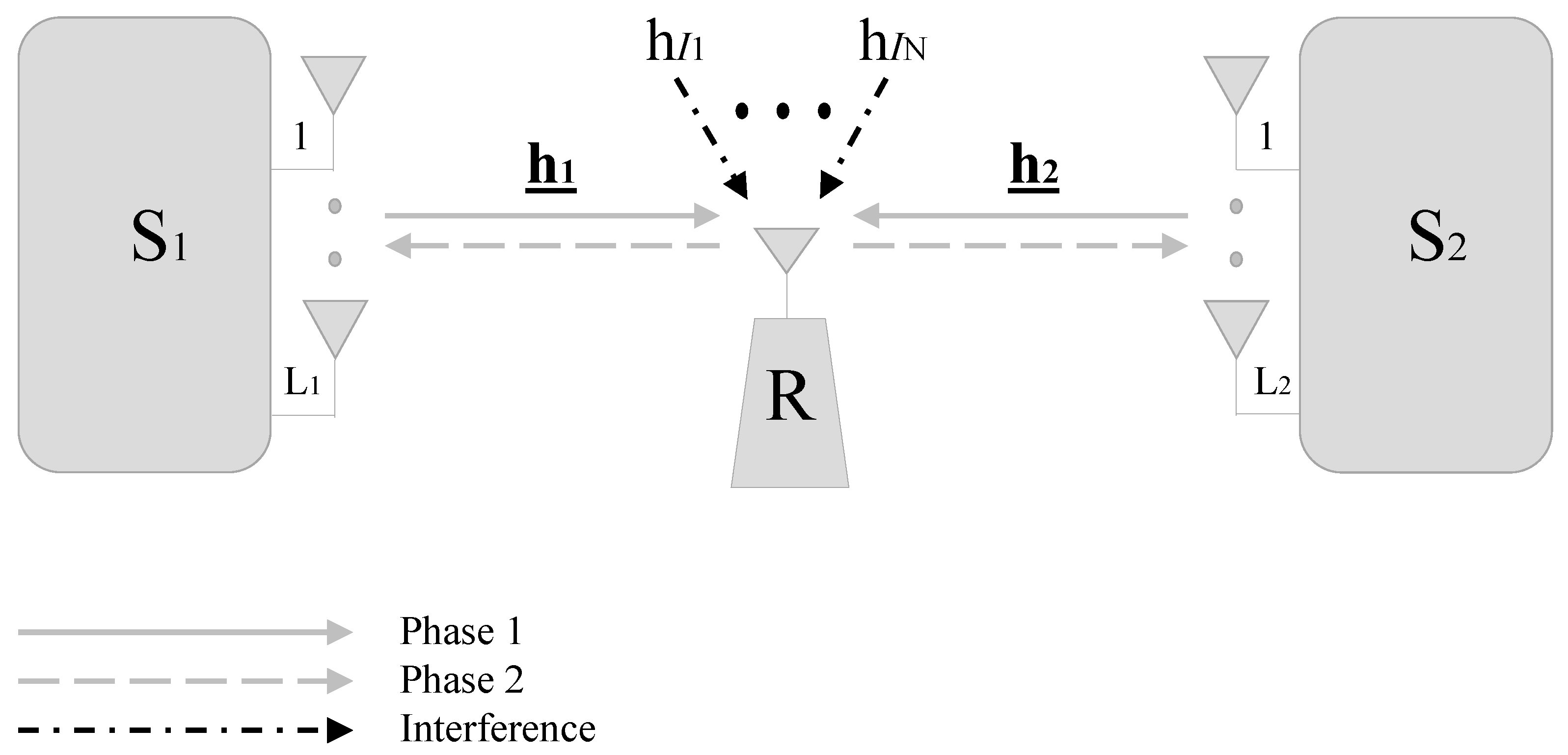
An AF-TWRN system with two source terminals and having and antennas respectively, is considered where sources communicate via a single antenna relay R which is exposed to N co-channel interference signals from other users in the network (In practice, a small size and low complexity user can behave as a relay to establish reliable links between two base stations in a cellular network (e.g., [1,20]), or between two routers in a WiFi network, or between two coordinators in a wireless sensor network when larger range and better energy efficiency are needed. If the selected user is close to the edge of cells/clusters, then the CCI level can be considerable compared to negligible CCI at two source terminals which can be at the center of neighboring cells [17].) as depicted in Figure 1. and are and channel vectors between and respectively. is the flat fading coefficient of i-th interference channel. The direct link between two source terminals is assumed to be unavailable due to large path loss and/or deep shadowing. Channel coefficients at each hop are modeled as independent and identically distributed (i.i.d) Rayleigh flat fading. For the performance analysis in the next section, the CSI is assumed to be available at both sources and at the relay, then, the effect of imperfect CSI is also explored later. The communication between two source terminals is divided into two phases. In the first phase, and transmit their unit energy signals and respectively by using MRT technique. Without loss of generality, all nodes are assumed to have equal transmit powers, and denote the power of interference signals as . Then, the received signal at the relay R can be written as follows
where exponential-decay path loss model is assumed with denoting the path loss exponent. Distances between and are shown as and , respectively. is the i-th unit energy interfering signal affecting R. In the second phase, the relay amplifies the sum of the received signals with a scaling factor G and then broadcasts to and . By using maximum ratio combining (MRC), the received signals at both sources can be expressed as
MRT weight vectors and are specified as and . Noise samples and elements of , vectors are modeled as complex additive white Gaussian noise with zero mean and variance . The relay scaling factor [17,26,27] is given as
Using channel reciprocity in TWRN, the two sources can cancel their self interference term (i.e., the effect of their transmitted signals). Substituting (1) in (2) and after some algebraic manipulations, the SINRs can be obtained as
where and are the instantaneous SNRs at and hops and is the instantaneous interference-to-noise power ratio (INR) at the relay.
3. Performance Analysis
In this section, first, upper bounds of CDFs of the SINRs for the sources and e2e system are obtained. Secondly, lower bounds of OP and SER expressions are derived. Then asymptotic OP and SER analyses are carried out, thus diversity and array gains are provided. Finally, the upper bound of ergodic sum rate and the effect of CEE are presented.
Since it is mathematically intractable to obtain the exact performance results for TWRNs with CCI, similar to previous studies [16,17,18,19,20], upper bounds on and in (4) can be written as
Then, CDFs of the random variables and can be expressed as
Note that the instantaneous SNRs, and are central Chi-square distributed random variables with and degrees of freedom, respectively. Then their PDF and CDF are given as [21]
where is the Gamma function ([28] [eqn 8.339.1]). Average SNRs are denoted as and using . Similarly, is distributed as central Chi-square random variable with degrees of freedom where its PDF is [16]
where average INR is shown as . By substituting (10) and (11) into (6) and after several algebraic manipulations to solve the integral, (6) is equivalently expressed as
where and is the Tricomi confluent hypergeometric function (The Tricomi confluent hypergeometric function and the Meijer’s G-function can easily evaluated numerically by using well-known software programs such as MAPLE or MATHEMATICA.), defined by the integral ([28] [eqn 9.211.4]). To this end, the CDF of can be derived as
Finally, the end-to-end SINR of the system can be expressed as [19]
In the literature, some papers (e.g., [16]) have derived performance expressions based on , however, it is not the correct e2e SINR of two-way relaying systems. The upper bound CDF of e2e SINR can be derived by using (16) as follows
The computation of this CDF is highly complicated since and are correlated as they contain common random variables , and . To this end, similar to [26], the following Lemma is introduced.
Lemma 1.
SINRs for and can be further upper bounded by dividing (4) to and as follows
due to the fact that both and .
With the help of this new bound, (17) can be simplified to its conditioned version depending only on
Then, the unconditional CDF of can be derived as
The detailed derivation is shown in Appendix A.
This closed form upper bound on CDF of e2e SINR is in a simple form with the help of Lemma 1. In addition, for the case of no interference, i.e., , the CDF can be reduced to
3.1. System Outage Probability
The outage probability for is defined as the probability that SINR for the link falls below a threshold , where and . System outage on the other hand can be defined as at least one of the source nodes being in outage. As a result, the lower bound on system OP is actually the CDF of random variable evaluated at and can be written as
3.2. Sum Symbol Error Rate
SSER can be defined as the summation of SER at and nodes, and it is another important performance criterion in TWRNs. Mathematically, it can be expressed as [29]
For several signal constellations employed in practical systems, the SER can be written as where a and b are modulation coefficients, i.e., for BFSK modulation, for BPSK and for M-ary PAM. Then SER can be evaluated by using the CDF-based approach [18] as
To simplify the derivation of (24), CDFs of and can be expressed in a more tractable form. The mathematical identity ([30] [eqn 13.2.8]) where is Pochhammer’s symbol, can help expanding the Tricomi confluent hypergeometric function to a finite sum series. After substitution the simplified versions of (14) and (15) in (24) with some mathematical manipulations and by utilizing ([28] [eqn 9.211.4]), the lower bound of SER for and can be expressed as (In the sequel, OP, SER and ESR for any source can be obtained by replacing the subscript i and j with such that .)
furthermore, it is worth mentioning that for no interference case, the SER in (25) can be simplified as
By substituting the SER of and into (23), the lower bound of SSER can be easily obtained in closed-form.
3.3. Asymptotic Analysis
In this subsection, in order to extract the diversity and array gains, and are simplified by assuming high SNR values (i.e.,). Using the Maclaurin series expansion of the exponential function [31]. The PDF of and in (7) and (8) can be approximated respectively as
Then, by integrating these PDFs with respect to x and y, CDFs can be written as follows
Recall that step in both (13) and (19) can be simplified by ignoring the last multiplication term; and . To this end, by using these approximations, following the same procedure and after some mathematical manipulations, asymptotic CDFs for , and can be given as
For the interference-free system, (32) becomes
Furthermore, by substituting the asymptotic CDFs of and in (24) with the help of ([30] [eqn 13.2.8]) and some mathematical simplifications, asymptotic expressions of SER for and can be derived as
Having this result, the asymptotic SSER can be directly obtained from (23). As a special case, asymptotic SERs for and in interference-free system are provided as
In order to find the asymptotic system OP expression, both ([32] [Prop. 5]) and (32) are used where is replaced with and a large value of is assumed. Then, can be obtained as
where H.O.T denotes high order terms and the scaling factor is given as
Furthermore, by using as described in [32], the diversity gain and the array gain can be written as
Note that, even though CCI degrades the array gain considerably, it does not decrease the diversity gain.
3.4. Ergodic Sum Rate
The ergodic sum rate which is measured by bits/s/Hz, is an important performance indicator as it can provide insight about the maximum transmission rate. For TWRNs, it is expressed as the summation of the ergodic rates of and , and thus for our system model, it can be written as [17,23]
where the factor 1/2 appears since data exchange needs two time slots. To the best of our knowledge, the closed form solution of the above expression can not be obtained. However, an approximate expression for the ergodic sum rate can be derived using the Jensen’s inequality (Jensen’s inequality: Suppose that X is a random variable with expectation , and function g is convex and finite. Then ([33] [eqn 5.5]).). Specifically, an upper bound on the ergodic sum rate in (39) is obtained as
where and can be obtained as
The detailed derivation is shown in Appendix B.
3.5. Impact of Channel Estimation Errors
In practice, channel coefficients are estimated at the receiver and thereby, can not be known perfectly. Channel estimation errors depend on the type of the estimator and the number of pilot symbols. In general, by using linear minimum mean square error (MMSE), the channel coefficients can be modeled as [18]
where the estimation error , and channel estimates and are assumed to be mutually independent and follow complex Gaussian distribution with zero mean and variances , , and , respectively. Note that MRT based weight vectors become and . Substituting (42) into (1), (2) and (3), and after removing the self-interference term with some further simplifications, the instantaneous SINRs can be written as
where, , , , , , , and . It is worth mentioning that and reflect the amount of estimation error. When , perfect CSI is used and (43) becomes equal to (4). Channel estimation errors are usually small in practical operations, thus , , and can be neglected (as in [34,35]), since their values are much smaller compared to the SNR values and in the denominator. Then, (43) can be written as
Although not shown here, by using Monte Carlo simulations the mean square error between (43) and (44) is observed to be close to zero for a wide SNR ranges when ≤ 0.01. Therefore, this SINR approximation can be safely used. Accordingly, the upper bound given in (5) becomes
Using this result and following the same derivation steps, CDFs of source SINRs, and can be obtained as
Furthermore, by applying Lemma 1 with some mathematical manipulations with the help of ([28] [eqn 1.111 and 3.351.3]), the CDF of e2e SINR can be derived as
By utilizing the CDF expressions in (46) and (47), OP, SER and ESR can be easily derived in the presence of channel estimation errors similar to perfect CSI case. Although the lengthy derivations are not presented here to avoid repetition, the effect of channel estimation errors is illustrated and discussed in the next section.
4. Numerical Results and Discussion
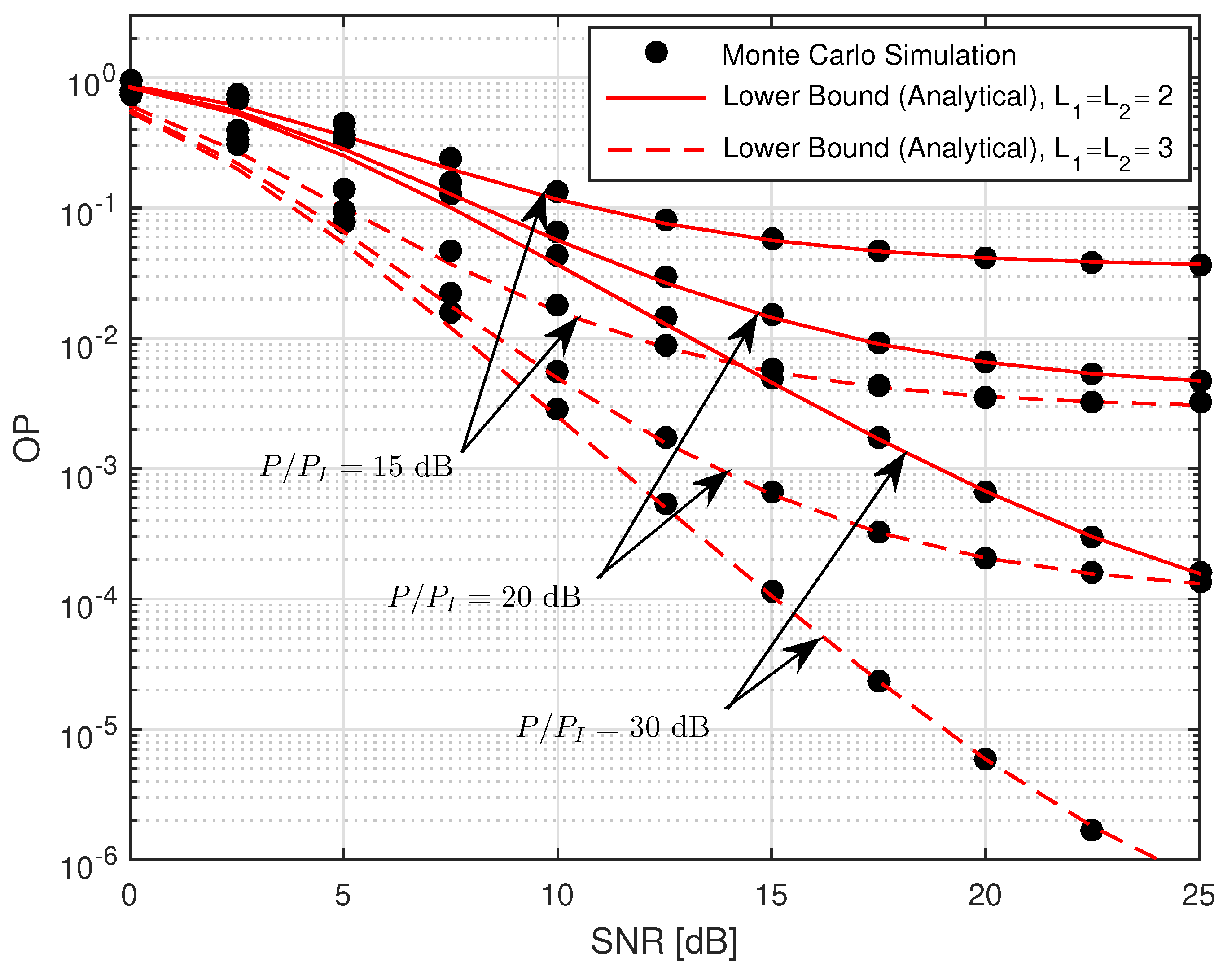
In this section, our analytical results are compared with Monte Carlo simulations. The OP curves are plotted by using (20) and (36), and the curves for the SSER are plotted based on (23). Plots of upper bound of ESR correspond to the expression in (40). For illustration purposes, the distances between each source and the relay are assumed to be identical and normalized to unity.
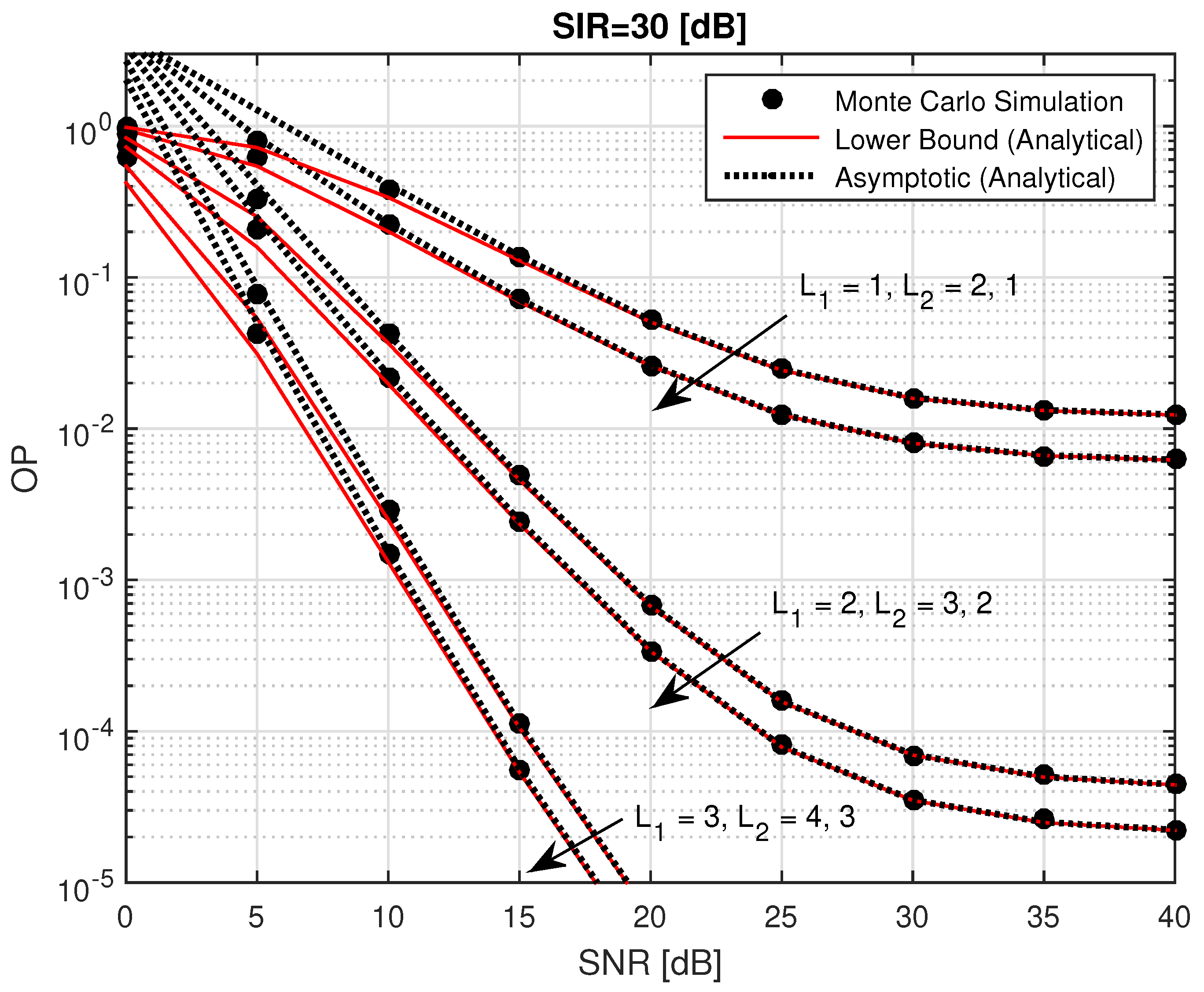
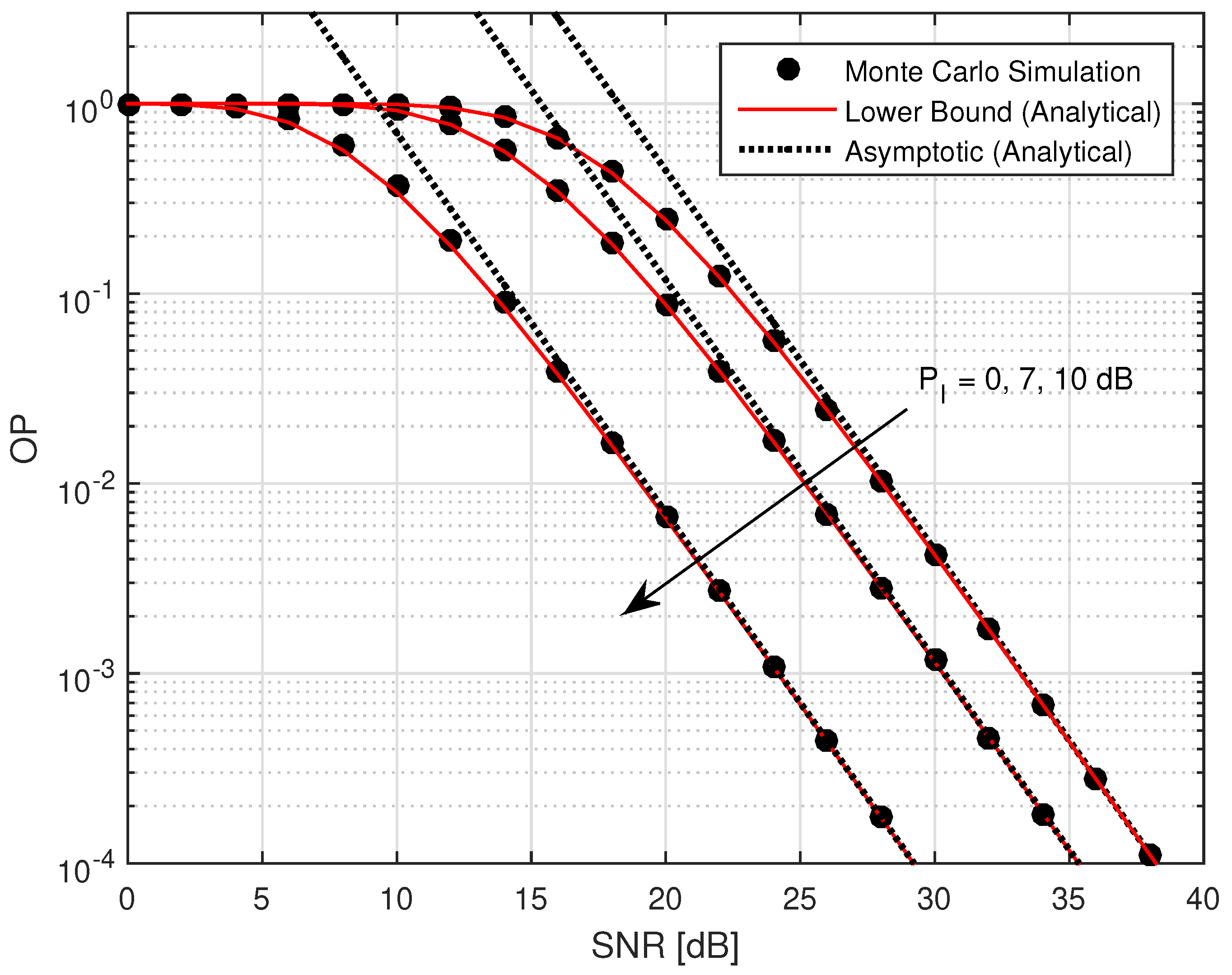
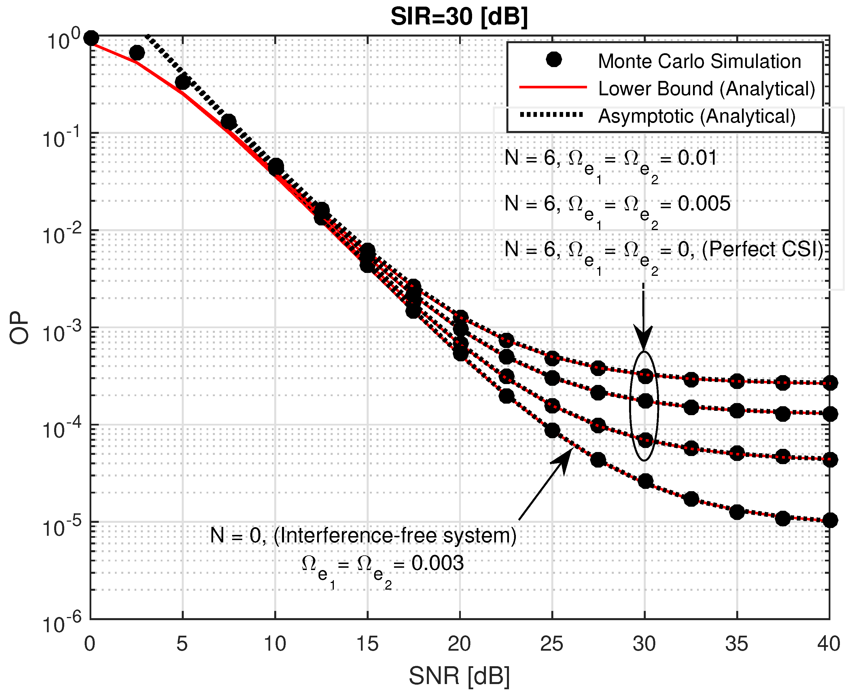
Figure 2 demonstrates the analytical lower bound for the system OP performance when different signal-to-interference power ratios (SIR) are utilized ( dB). Our theoretical results match the Monte Carlo simulation results perfectly in medium to high SNR range even for small SIR (note that in cellular system, the practical SIR value to provide sufficient voice quality is greater than or equal to 18 dB [36]). Figure 3 shows the system OP when the number of interference signals is and the SIR is ( dB). As can be observed, CCI significantly degrades the outage probability as the curves exhibit an error floor in the high SNR regime since the effect of interference becomes dominant compared to noise. In addition, to understand the effect of MRT on the performance, several number of antennas at and are selected as () =, , . As expected, for a fixed , increasing does not change the diversity gain e.g., () and () have the same diversity. Obviously, it can be inferred that employing MRT in AF-TWRN makes the system resilient against CCI and thus it is practically preferable to obtain availability and more.
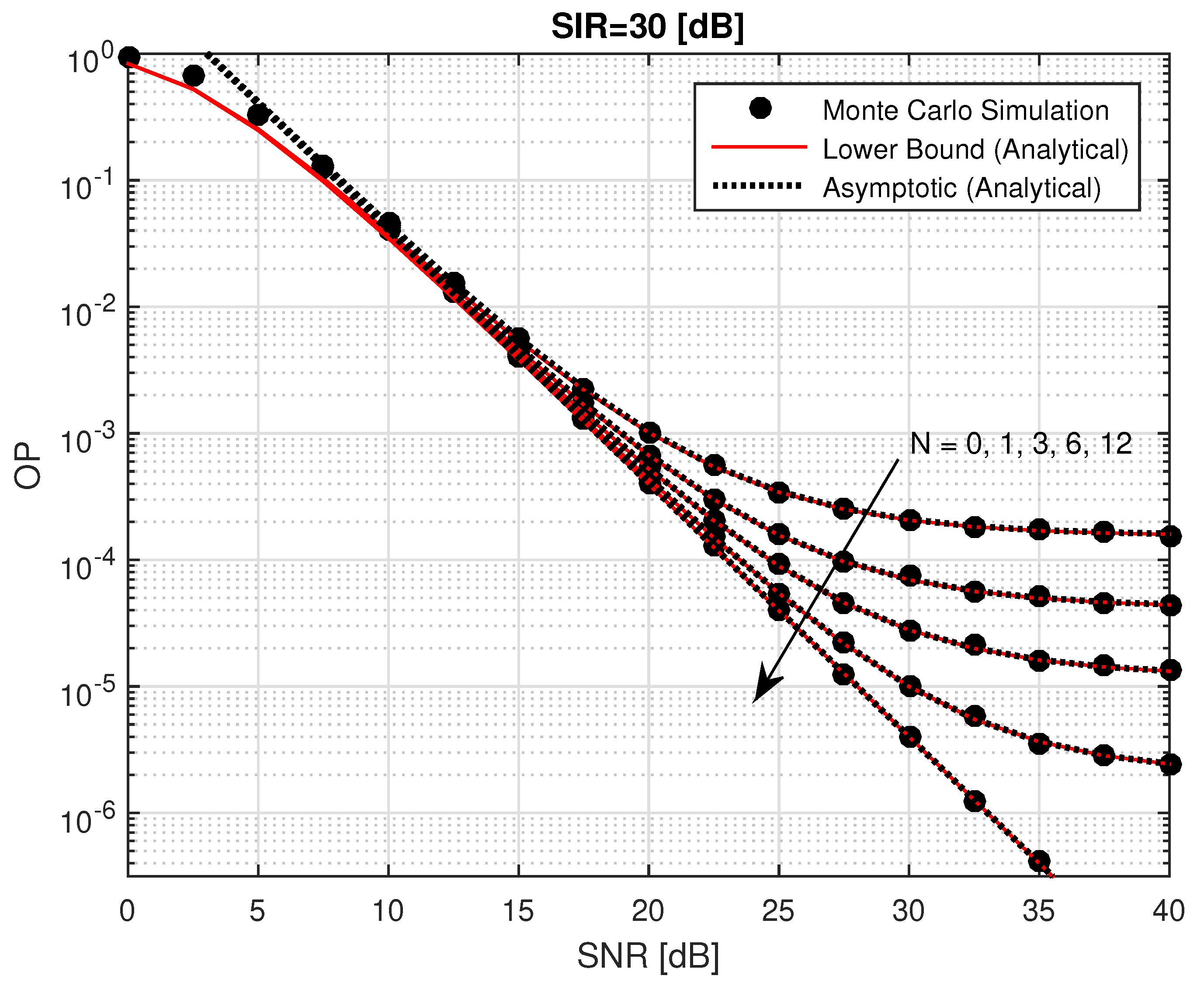
Figure 4 illustrates the impact of the number of CCI signals on the system OP while dB is kept constant and . As can be observed, by decreasing the number of CCI signals, the system OP decreases as well. When the SNR increases, the OP reaches to an error floor, while the error floor does not exist for the interference-free case. Figure 5 illustrates the effect of the strength of CCI signals on the system OP. The number of CCI signals is kept constant and various interference powers ( dB) are considered. It can be seen that the system OP increases when the interference power is increased. Besides, from Figure 4 and Figure 5, it can be understood that the change of the number and/or the power of interfering signals do not affect the diversity order.
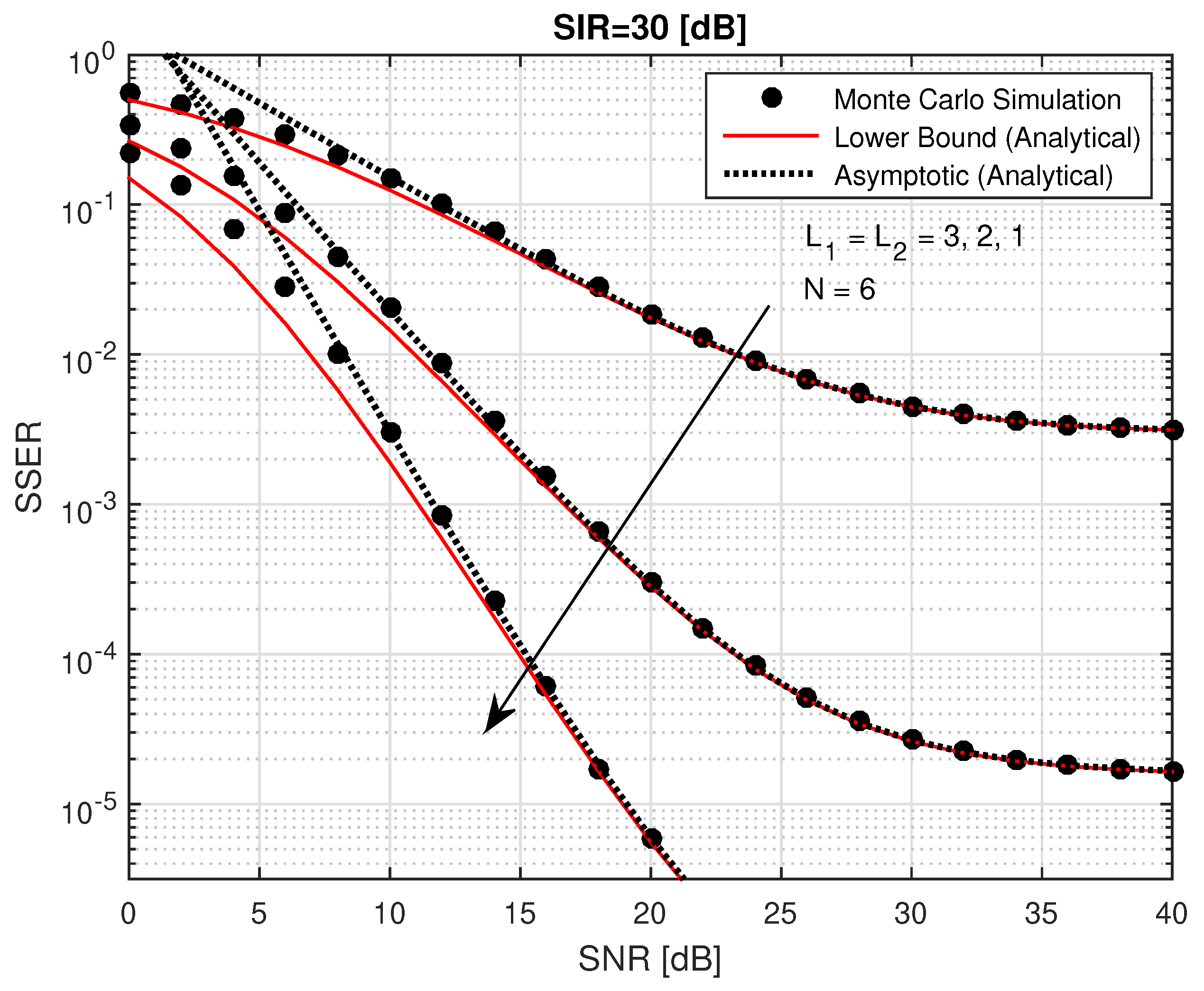
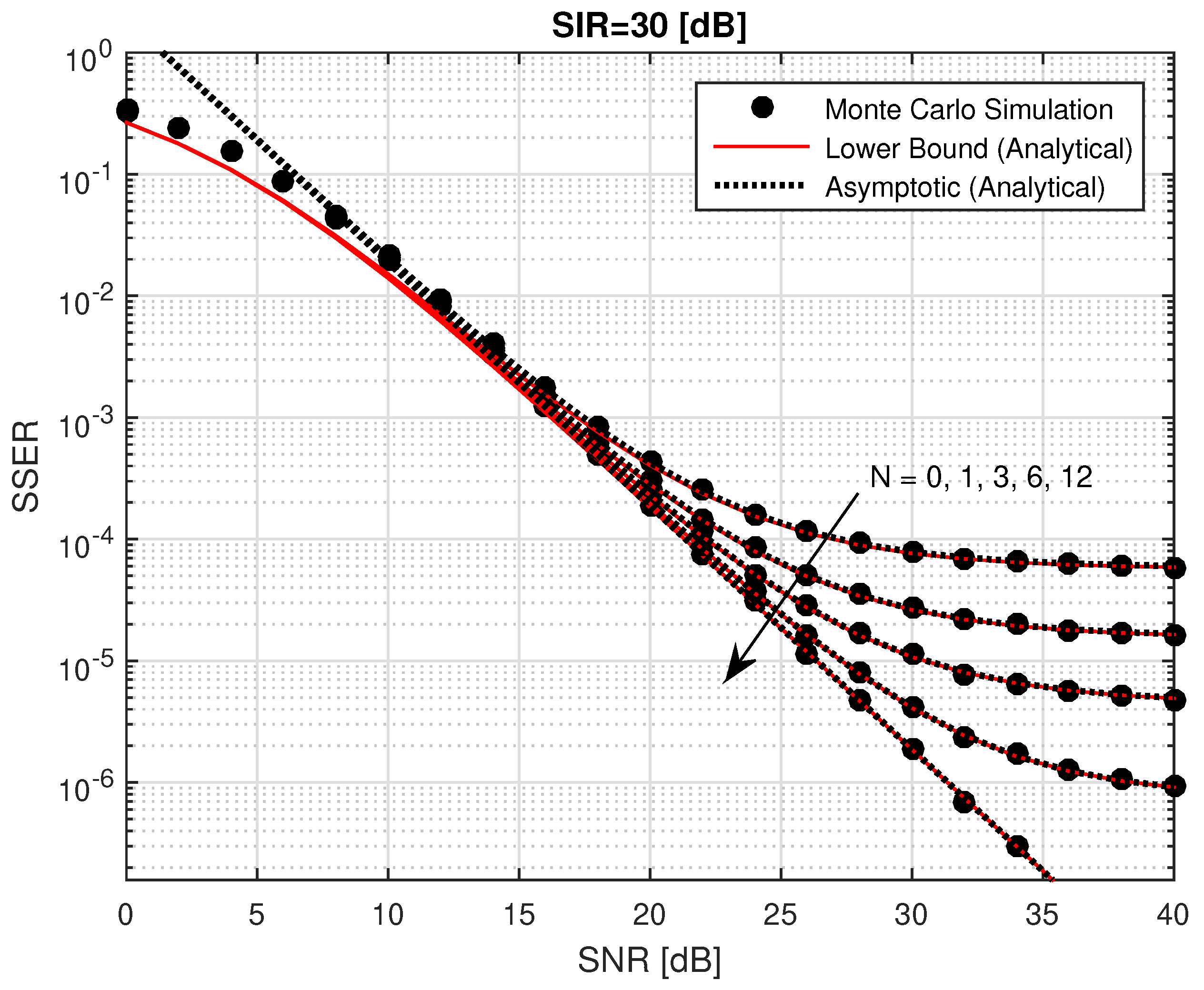
Figure 6 depicts the theoretical lower bound of the SSER for BPSK modulation () with different antenna numbers for and . As can be observed, the SSER can be improved dramatically by employing MRT (the cases when ) compared to the single antenna case (when ). Specifically, MRT with 2 or 3 antennas at both sources can achieve and SSER respectively at 15 dB SNR compared to SSER without MRT. Figure 7 demonstrates the impact of the number of CCI signals on the SSER. When the number of CCI signals is decreased, the SSER performance becomes better as the number of CCI have a direct influence on the system array gain with no change in the diversity order.
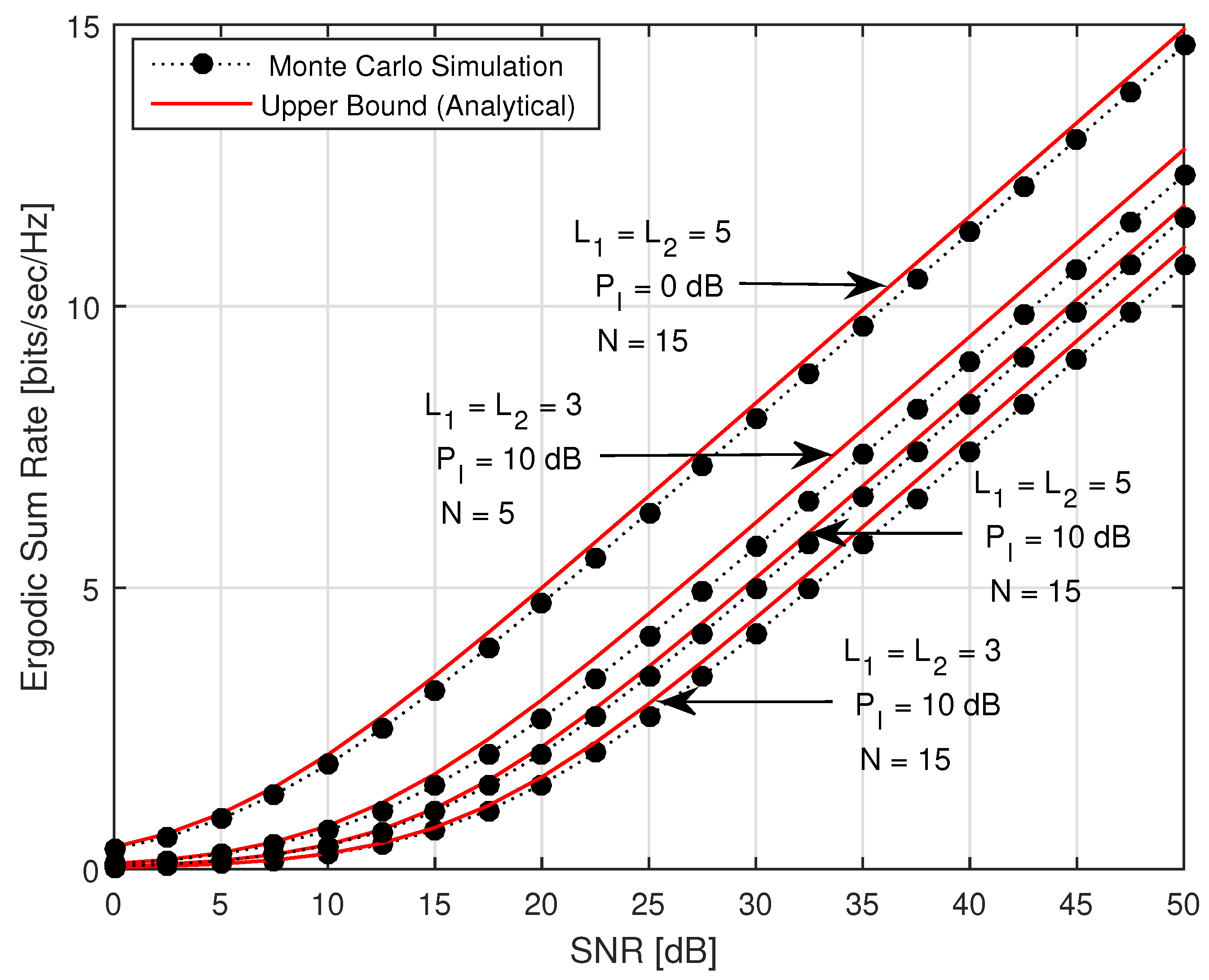
Figure 8 shows the ergodic sum rate of the system for several number of CCI signals, antennas and different levels of interference power. Our analytical ESR upper bound denoted by (40) is tight compared to simulation results. Obviously, increasing the number and/or the power of the CCI signals will degrade the ESR performance. On the other hand, increasing the number of antennas will improve the performance.
Figure 9 presents the effect of both CCI and CEE on the system OP performance for various values of CEE where the analytical lower bound results are calculated by using expression (47) and the ratio between the signal and interference power is assumed to be constant ( dB). As can be seen from the figure, the OP becomes worse when CEE increases. To overcome this problem, the number of pilot symbols can be increased. More links can be deployed in the proposed system to make it robust against the CCI and CEE. Figure 10 shows the impact of the number of antennas on OP where the noise power is normalized to unity where the transmit and interferer powers are fixed at dB and dB, respectively. Note that our analytical bounds are close to the exact results obtained by Monte Carlo simulations even at low SNRs when the interference power (see Figure 5) is assumed to be fixed. The plot indicates that the joint effect of CCI and CEE can be reduced considerably by utilizing MRT with increasing the number of antennas.
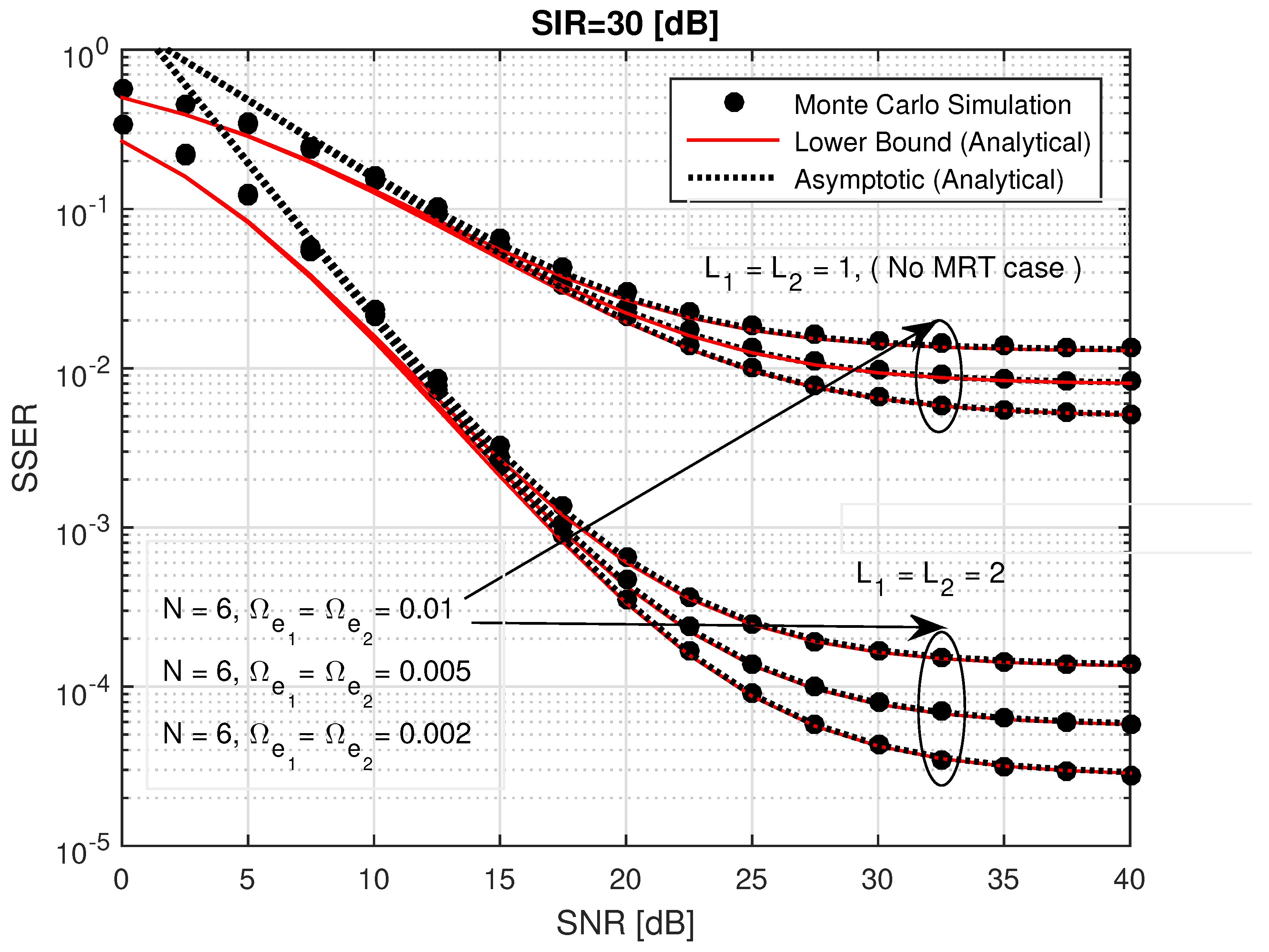
In Figure 11, the effect of imperfect channel estimation on the SSER performance is explored. As in Figure 6, SIR is assumed constant ( dB) and the single antenna case is compared with the multi-antenna case () when the number of CCI signals is fixed () and the values of CEE is varied. Clearly, in both cases, increasing amount of estimation errors affect only the array gain, thus the SSER becomes worse. However, using more antennas with MRT increases the diversity gain and SSER considerably. Employing the low complexity MRT technique can be a practical solution for the performance degradation observed in TWRNs due to CCI, noise and CEE.
5. Conclusions
In this paper, MRT technique is proposed as a solution for AF-TWRNs to suppress the performance loss caused by unavoidable CCI plus noise distortion at the single antenna relay receiver. After obtaining the upper bound of the cumulative distribution function of SINR, tight lower bound expressions of OP, SER and upper bound of system ergodic sum rate are derived and illustrated with extensive numerical examples. Moreover, the asymptotic behavior of the OP and SSER, the array and diversity gains are presented. Furthermore, the effect of imperfect CSI is also explored. Our derived expressions are validated for arbitrary signal-to-interference power ratios, numbers of co-channel interferers and a majority of modulation formats employed in the practical systems. The new proposed system can be highly desirable since using MRT allows employing low complexity relays for coverage extension and reliability enhancement in cellular, WiFi, sensor networks.
Author Contributions
The authors A.A. and T.G. contributed to the conceptualization, methodology, analysis, software, validation, writing and review. E.E. contributed to the software. The over all supervision and editing done by T.G.
Conflicts of Interest
The authors declare no conflict of interest.
Abbreviations
The following abbreviations are used in this manuscript:
| AF | amplify-and-forward |
| TWRNs | two-way relay networks |
| CCI | co-channel interference |
| SINR | signal-to-interference-plus-noise ratio |
| INR | interference-to-noise ratio |
| SIR | signal-to-interference ratio |
| MIMO | multiple-input multiple-output |
| MRT | maximal ratio transmission |
| MRC | maximum ratio combining |
| OP | outage probability |
| SER | symbol error rate |
| SSER | sum symbol error rate |
| ESR | ergodic sum rate |
| CEE | channel estimation error |
| MMSE | minimum mean square error |
| probability density function | |
| CDF | cumulative distribution function |
| CSI | channel state information |
Appendix A. Derivation of (20)
To begin with, recall that and . Besides, step of (19) is
where and are the complementary distribution function of and respectively. By substituting the CDFs of and from (9) and (10), (A1) can be written as
Then by averaging over the PDF of in (11) yields
Appendix B. Derivation of (41)
The statistical mean values of and can be determined by using the CDF-based method as
After applying the identity ([30] [eqn 13.2.8]) on (14) and (15), the Tricomi confluent hypergeometric function is expanded to a finite sum series as
References
- Shukla, M.K.; Yadav, S.; Purohit, N. Performance evaluation and optimization of traffic-aware cellular multiuser two-way relay networks over Nakagami-m fading. IEEE Syst. J. 2018, 12, 1933–1944. [Google Scholar] [CrossRef]
- Rankov, B.; Wittneben, A. Spectral efficient protocols for half-duplex fading relay channels. IEEE J. Sel. Areas Commun. 2007, 25, 379–389. [Google Scholar] [CrossRef]
- Popovski, P.; Yomo, H. Wireless network coding by amplify-and-forward for bi-directional traffic flows. IEEE Commun. Lett. 2007, 11, 16–18. [Google Scholar] [CrossRef] [Green Version]
- Rabie, K.M.; Adebisi, B.; Alouini, M.-S. Half-duplex and full-duplex AF and DF relaying with energy-harvesting in Log-Normal fading. IEEE Trans. Green Commun. Netw. 2017, 1, 468–480. [Google Scholar] [CrossRef]
- Bastami, A.H.; Habibi, S. Cognitive MIMO two-way relay network: Joint optimal relay selection and spectrum allocation. IEEE Trans. Veh. Technol. 2018, 67, 5937–5952. [Google Scholar] [CrossRef]
- Yue, X.; Liu, Y.; Kang, S.; Nallanathan, A.; Chen, Y. Modeling and analysis of two-way relay non-orthogonal multiple access systems. IEEE Trans. Commun. 2018, 66, 3784–3796. [Google Scholar] [CrossRef]
- Peng, C.; Li, F.; Liu, H. Wireless Energy Harvesting Two-Way Relay Networks with Hardware Impairments. Sensors 2017, 17, 2604. [Google Scholar] [CrossRef] [PubMed]
- Guo, K.; An, K.; Zhang, B.; Guo, D. Performance Analysis of Two-Way Satellite Multi-Terrestrial Relay Networks with Hardware Impairments. Sensors 2018, 18, 1574. [Google Scholar] [CrossRef]
- Sun, C.; Liu, K.; Zheng, D.; Ai, W. Secure Communication for Two-Way Relay Networks with Imperfect CSI. Entropy 2017, 19, 522. [Google Scholar] [CrossRef]
- Xia, X.; Zhang, D.; Xu, K.; Xu, Y. A comparative study on interference-limited two-way transmission protocols. J. Commun. Netw. 2016, 18, 351–363. [Google Scholar]
- Lei, L.; Lagunas, E.; Chatzinotas, S.; Ottersten, B. NOMA aided interference management for full-duplex self-backhauling HetNets. IEEE Commun. Lett. 2018, 22, 1696–1699. [Google Scholar] [CrossRef]
- Ghasemi, A.; Sousa, E.S. Spectrum sensing in cognitive radio networks: Requirements, challenges and design trade-offs. IEEE Commun. Mag. 2008, 46, 32–39. [Google Scholar] [CrossRef]
- Liang, X.; Jin, S.; Wang, W.; Gao, X.; Wong, K.K. Outage probability of amplify-and-forward two-way relay interference-limited systems. IEEE Trans. Veh. Technol. 2012, 61, 3038–3049. [Google Scholar] [CrossRef]
- Liang, X.; Jin, S.; Gao, X.; Wong, K.K. Outage performance for decode-and-forward two-way relay network with multiple interferers and noisy relay. IEEE Trans. Commun. 2013, 61, 521–531. [Google Scholar] [CrossRef]
- Xia, X.; Zhang, D.; Xu, K.; Xu, Y. Interference-limited two-way DF relaying: Symbol-error-rate analysis and comparison. IEEE Trans. Veh. Technol. 2014, 63, 3474–3480. [Google Scholar] [CrossRef]
- Ikki, S.S.; Aissa, S. Performance analysis of two-way amplify-and-forward relaying in the presence of co-channel interferences. IEEE Trans. Commun. 2012, 60, 933–939. [Google Scholar] [CrossRef]
- Da Costa, D.B.; Ding, H.; Yacoub, M.D.; Ge, J. Two-way relaying in interference-limited AF cooperative networks over Nakagami-m fading. IEEE Trans. Veh. Technol. 2012, 61, 3766–3771. [Google Scholar] [CrossRef]
- Yang, L.; Qaraqe, K.; Serpedin, E.; Alouini, M.-S. Performance analysis of amplify-and-forward two-way relaying with co-channel interference and channel estimation error. IEEE Trans. Commun. 2013, 61, 2221–2231. [Google Scholar] [CrossRef]
- Soleimani-Nasab, E.; Matthaiou, M.; Ardebilipour, M.; Karagiannidis, G.K. Two-way AF relaying in the presence of co-channel interference. IEEE Trans. Commun. 2013, 61, 3156–3169. [Google Scholar] [CrossRef]
- Shukla, M.K.; Yadav, S.; Purohit, N. Cellular multiuser two-way relay network with cochannel interference and channel estimation error: Performance analysis and optimization. IEEE Trans. Veh. Technol. 2018, 67, 3431–3446. [Google Scholar] [CrossRef]
- Lo, T.K.Y. Maximum ratio transmission. IEEE Trans. Commun. 1999, 47, 1458–1461. [Google Scholar] [CrossRef]
- Yang, N.; Yeoh, P.L.; Elkashlan, M.; Collings, I.B.; Chen, Z. Two-way relaying with multi-antenna sources: Beamforming and antenna selection. IEEE Trans. Veh. Technol. 2012, 61, 3996–4008. [Google Scholar] [CrossRef]
- Yadav, S.; Upadhyay, P.K.; Prakriya, S. Performance evaluation and optimization for two-way relaying with multi-antenna sources. IEEE Trans. Veh. Technol. 2014, 63, 2982–2989. [Google Scholar] [CrossRef]
- Erdogan, E.; Gucluoglu, T. Performance analysis of maximal ratio transmission with relay selection in two-way relay networks over Nakagami-m fading channels. Wirel. Person. Commun. 2016, 88, 185–201. [Google Scholar] [CrossRef]
- Guo, K.; Guo, D.; Zhang, B. Performance analysis of two-way multi-antenna multi-relay networks with hardware impairments. IEEE Access 2017, 5, 15971–15980. [Google Scholar] [CrossRef]
- Erdogan, E.; Gucluoglu, T. Simple outage probability bound for two-way relay networks with joint antenna and relay selection over Nakagami-m fading channels. Electron. Lett. 2015, 51, 415–417. [Google Scholar] [CrossRef]
- Hasna, M.O.; Alouini, M.-S. End-to-end performance of transmission systems with relays over rayleigh-fading channels. IEEE Trans. Wirel. Commun. 2003, 2, 1126–1131. [Google Scholar] [CrossRef]
- Gradshteyn, I.S.; Ryzhik, I.M.; Jeffrey, A.; Zwillinger, D. Table of Integrals, Series, and Products, 7th ed.; Elsevier Academic Press: New York, NY, USA, 2005. [Google Scholar]
- Louie, R.H.Y.; Li, Y.; Vucetic, B. Practical physical layer network coding for two-way relay channels: Performance analysis and comparison. IEEE Trans. Wirel. Commun. 2010, 9, 764–777. [Google Scholar] [CrossRef]
- Olver, F.W.J.; Lozier, D.W.; Boisvert, R.F.; Clark, C.W. NIST Handbook of Mathematical Functions; Cambridge University Press: New York, NY, USA, 2010. [Google Scholar]
- Huang, Y.; Al-Qahtani, F.; Zhong, C.; Wu, Q.; Wang, J.; Alnuweiri, H. Performance analysis of multiuser multiple antenna relaying networks with co-channel interference and feedback delay. IEEE Trans. Commun. 2014, 62, 59–73. [Google Scholar] [CrossRef]
- Zhengdao, W.; Giannakis, G.B. A simple and general parameterization quantifying performance in fading channels. IEEE Trans. Commun. 2003, 51, 1389–1398. [Google Scholar] [CrossRef]
- Van Mieghem, P. Performance Analysis of Communications Networks and Systems; Cambridge University Press: New York, NY, USA, 2006. [Google Scholar]
- Wang, C.; Liu, T.C.K.; Dong, X. Impact of channel estimation error on the performance of amplify-and-forward two-way relaying. IEEE Trans. Veh. Technol. 2012, 61, 1197–1207. [Google Scholar] [CrossRef]
- Wang, L.; Cai, Y.; Yang, W. On the finite-SNR DMT of two-way AF relaying with imperfect CSI. IEEE Wirel. Commun. Lett. 2012, 1, 161–164. [Google Scholar] [CrossRef]
- Rappaport, T.S. Wireless Communications: Principles and Practice, 6th ed.; Prentice Hall PTR: Upper Saddle River, NJ, USA, 2002. [Google Scholar]
- Prudnikov, A.P.; Brychkov, Y.A.; Marichev, O.I. Integrals and Series, Volume 3; Gordon and Breach: New York, NY, USA, 1990. [Google Scholar]
Figure 1.
Block diagram of TWRN with maximal ratio transmission and CCI at the relay.

Figure 2.
System outage probability considering different SIR values, dB and .

Figure 3.
System outage probability of AF-TWRN with CCI for different number of antennas, dB.

Figure 4.
System outage probability of AF-TWRN with different numbers of co-channel interference signals, dB and .
Figure 4.
System outage probability of AF-TWRN with different numbers of co-channel interference signals, dB and .

Figure 5.
System outage probability with different values for the constant interference power, dB and .
Figure 5.
System outage probability with different values for the constant interference power, dB and .

Figure 6.
Sum SER performance of AF-TWRN with CCI for different number of antennas.

Figure 7.
Sum SER performance of AF-TWRN with CCI for different number of interference signals, .

Figure 8.
Achievable sum rate with different numbers of CCI Signals, power and different number of antennas.
Figure 8.
Achievable sum rate with different numbers of CCI Signals, power and different number of antennas.

Figure 9.
System outage probability of AF-TWRN with CCI and different CEE values, dB and .

Figure 10.
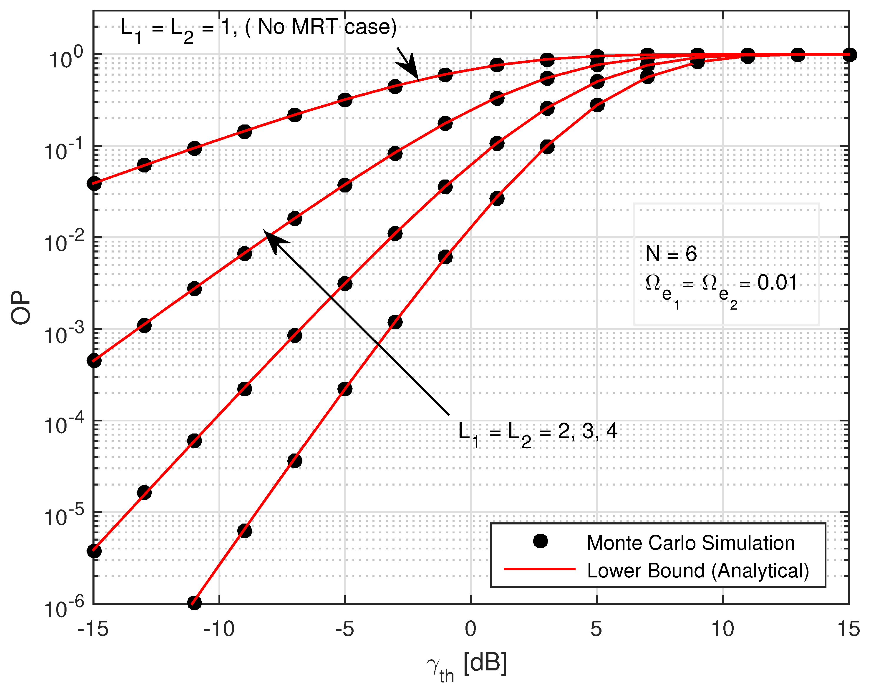
System outage probability vs SINR threshold for different number of antennas, dB and .

Figure 11.
Sum SER performance of AF-TWRN with different number of antennas, different values of CEE, dB and .
Figure 11.
Sum SER performance of AF-TWRN with different number of antennas, different values of CEE, dB and .

© 2019 by the authors. Licensee MDPI, Basel, Switzerland. This article is an open access article distributed under the terms and conditions of the Creative Commons Attribution (CC BY) license (http://creativecommons.org/licenses/by/4.0/).
Share and Cite
MDPI and ACS Style
Aladwani, A.; Erdogan, E.; Gucluoglu, T. Impact of Co-Channel Interference on Two-Way Relaying Networks with Maximal Ratio Transmission. Electronics 2019, 8, 392. https://doi.org/10.3390/electronics8040392
AMA Style
Aladwani A, Erdogan E, Gucluoglu T. Impact of Co-Channel Interference on Two-Way Relaying Networks with Maximal Ratio Transmission. Electronics. 2019; 8(4):392. https://doi.org/10.3390/electronics8040392
Chicago/Turabian StyleAladwani, Awfa, Eylem Erdogan, and Tansal Gucluoglu. 2019. "Impact of Co-Channel Interference on Two-Way Relaying Networks with Maximal Ratio Transmission" Electronics 8, no. 4: 392. https://doi.org/10.3390/electronics8040392
Note that from the first issue of 2016, this journal uses article numbers instead of page numbers. See further details here.