A Comprehensive Medical Decision–Support Framework Based on a Heterogeneous Ensemble Classifier for Diabetes Prediction

 ,
, 
 and
and
Abstract
:1. Introduction
- An efficient ensemble of heterogeneous classifiers is proposed based on extensive evaluations. This ensemble comprises seven of the well-known techniques: KNN, NB, FDT, ANN, SVM, LR, and DT. A set of preprocessing steps is performed to enhance the quality of the sub-datasets, including feature selection, missing value imputation, normalization, codification, and discretization. The framework was applied to DM diagnosis.
- The proposed framework used different base classifiers with varying lists of features. Each classifier has been evaluated with every sub-dataset and with different feature selection technique. The best algorithm is selected for every sub-dataset according to its performance.
- The ensemble framework uses a combination of bagging and random subspace techniques, with a weighted voting scheme based on F-measure other than accuracy, to prevent possibly biased results.
- The proposed classifier was evaluated by comparing its results with state-of-the-art individual and ensemble classifiers to prove its superiority.
2. Related Work
2.1. Single Classifiers
2.2. Ensembles of Multiple Classifiers
3. Materials and Methods
3.1. Dataset Description
3.2. Base Classifier Algorithms
3.2.1. Decision Tree
3.2.2. Support Vector Machine
3.2.3. Naïve Bayes
- For training set of cases and their associated class labels, each case is represented by a vector of n-dimensional attributes, = (, ,..., ) for values of features (, ,..., ). Each case can be classified as one of the classes: , ,..., .
- For a new case, , NB predicts that has the class having the highest a posteriori probability, conditioned on . In other words, the NB classifier predicts that case belongs to a class if and only if in Equation (5) is the largest, and is the maximum a posteriori hypothesis:Based on Bayes’ theorem, is calculated with Equation (6):
- Only needs to be optimized or maximized because has the same value for all classes, and if the class prior probabilities are not known, then, it is usually assumed that all classes have the same probability value, = = ... = .
- Datasets are usually of multiple attributes, so it would be computationally extremely expensive to compute . Using the naive assumption of class conditional independence, is calculated with Equation (7), and is calculated according to the type of the feature:
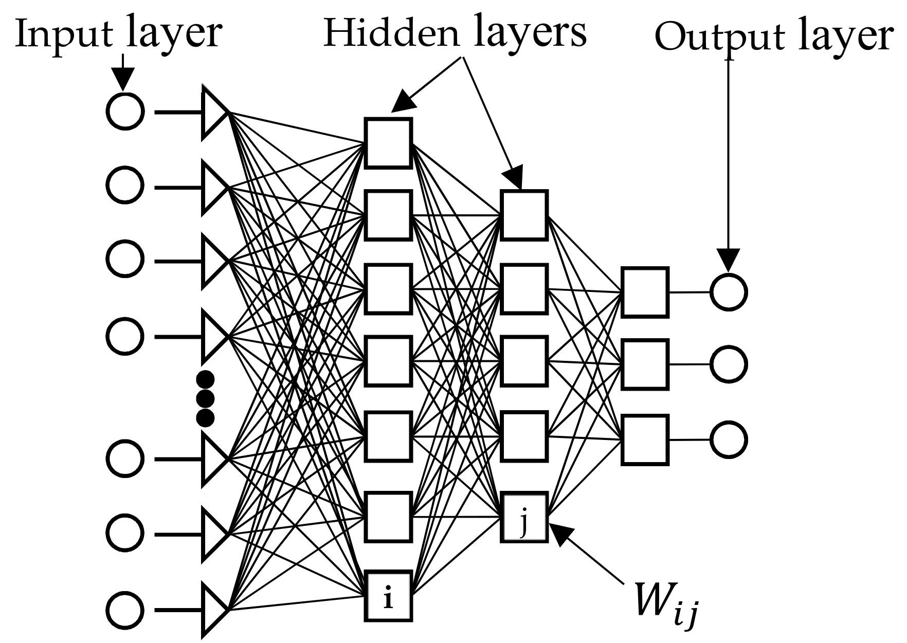
3.2.4. Artificial Neural Network
- (1)
- Calculate the weighted sum and add a bias term () according to Equation (8):
- (2)
- Transform through a suitable mathematical transfer function, such as unit step (threshold), piecewise linear and Gaussian sigmoid, or sigmoid (given in Equation (9); and
- (3)
- Transfer the result to neurons in the next layer until it reaches the output nodes (feed-forward):
3.2.5. Logistic Regression
3.2.6. Fuzzy Decision Tree
3.2.7. K-Nearest Neighbors
3.3. Classifier Ensembles
4. The Proposed Diabetes Ensemble Classifier
4.1. Domain and Data Understanding
4.2. Data Preprocessing
4.3. Data Distribution
4.4. Building the Ensemble Classifier
4.4.1. Feature Selection
| Algorithm 1. Construction of an enhanced ensemble classifier. |
Input:
|
4.4.2. Selecting and Building Base Classifiers
4.4.3. Ensemble of Base Classifiers
5. Results and Discussion
5.1. Evaluation Metrics
5.2. Evaluation Results
5.2.1. Base Classifier Evaluations Based on CFS
5.2.2. Base Classifier Evaluation Based on Wrapper FS
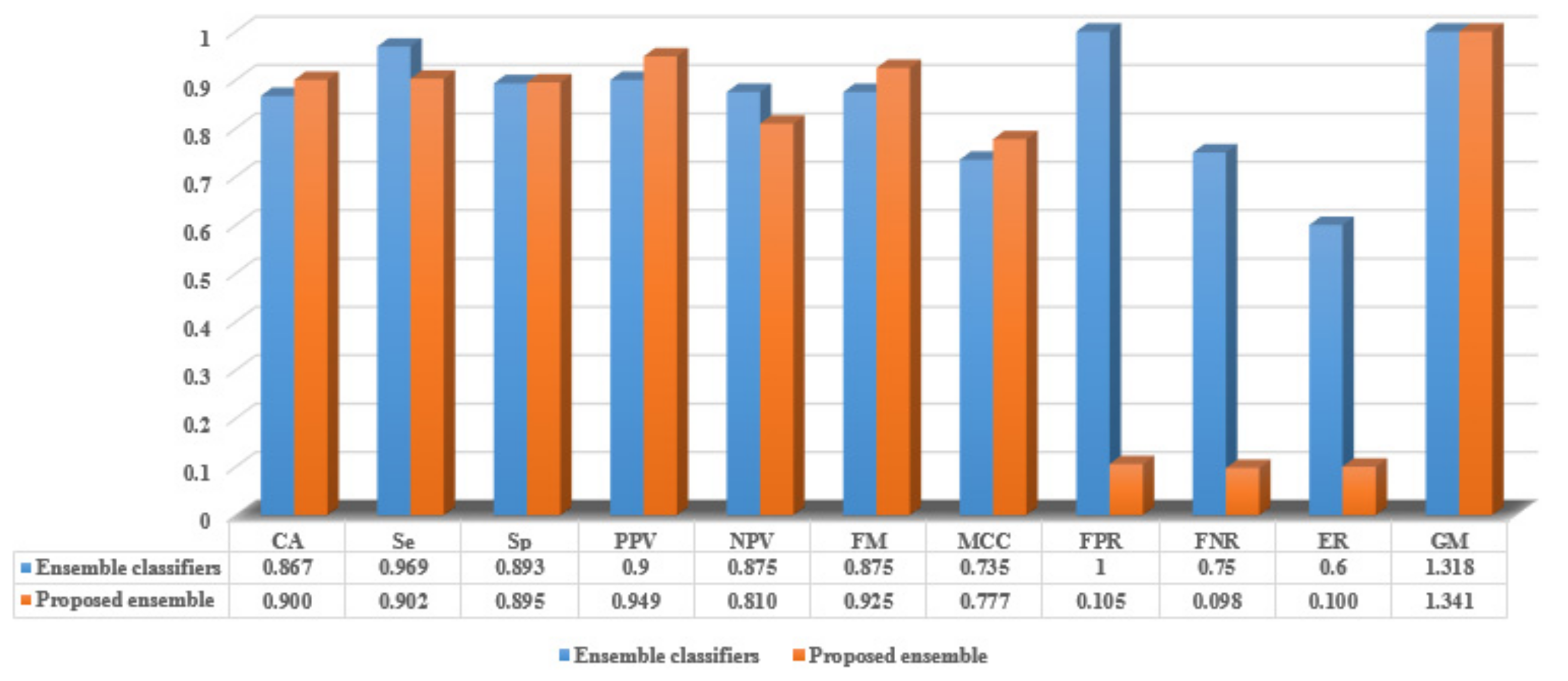
5.2.3. The Proposed Ensemble Evaluation
6. Conclusions
Author Contributions
Funding
Acknowledgments
Conflicts of Interest
References
- Zarkogianni, K.; Litsa, E.; Mitsis, K.; Wu, P.Y.; Kaddi, C.D.; Cheng, C.W.; Wang, M.D.; Nikita, K.S. A Review of Emerging Technologies for the Management of Diabetes Mellitus. IEEE Trans. Biomed. Eng. 2015, 62, 2735–2749. [Google Scholar] [CrossRef] [PubMed] [Green Version]
- Upadhyaya, S.; Farahmand, K.; Baker-Demaray, T. Comparison of NN and LR classifiers in the context of screening native American elders with diabetes. Expert Syst. Appl. 2013, 40, 5830–5838. [Google Scholar] [CrossRef]
- Guariguata, L.; Whiting, D.; Hambleton, I.; Beagley, J.; Linnenkamp, U.; Shaw, J. Global estimates of diabetes prevalence in adults for 2013 and projections for 2035 for the IDF Diabetes Atlas. Diabetes Res. Clin. Pract. 2014, 2, 137–149. [Google Scholar] [CrossRef] [PubMed]
- Zheng, T.; Xie, W.; Xu, L.; He, X.; Zhang, Y.; You, M.; Yang, G.; Chen, Y. A machine learning-based framework to identify type 2 diabetes through electronic health records. Int. J. Med. Inform. 2017, 97, 120–127. [Google Scholar] [CrossRef] [PubMed]
- Tripathi, B.; Srivastava, A. Diabetes mellitus complications and therapeutics. Med. Sci Monit. 2006, 12, RA130–RA147. [Google Scholar] [PubMed]
- Heydari, M.; Teimouri, M.; Heshmati, Z.; Alavinia, S. Comparison of various classification algorithms in the diagnosis of type 2 diabetes in Iran. Int. J. Diabetes Dev. Ctries. 2016, 36, 167–173. [Google Scholar] [CrossRef]
- Wei, W.Q.; Leibson, C.L.; Ransom, J.E.; Kho, A.N.; Chute, C.G. The absence of longitudinal data limits the accuracy of high-throughput clinical phenotyping for identifying type 2 diabetes mellitus subjects. Int. J. Med. Inf. 2013, 82, 239–247. [Google Scholar] [CrossRef]
- Bashir, S.; Qamar, U.; Khan, F. IntelliHealth: A medical decision support application using a novel weighted multi-layer classifier ensemble framework. J. Biomed. Inf. 2016, 59, 185–200. [Google Scholar] [CrossRef] [Green Version]
- Kavakiotis, I.; Tsave, O.; Salifoglou, A.; Maglaveras, N.; Vlahavas, I.; Chouvarda, I. Machine Learning and Data Mining Methods in Diabetes Research. Comput. Struct. Biotechnol. J. 2017, 15, 104–116. [Google Scholar] [CrossRef]
- Meng, X.; Huang, Y.; Rao, D.; Zhang, Q.; Liu, Q. Comparison of three data mining models for predicting diabetes or prediabetes by risk factors. Kaohsiung J. Med. Sci. 2013, 29, 93–99. [Google Scholar] [CrossRef] [Green Version]
- Marinov, M.; Mosa, A.; Yoo, I.; Boren, S.A. Data mining technologies for diabetes: A systematic review. J. Diabetes Sci. Technol. 2011, 5, 1549–1556. [Google Scholar] [CrossRef] [PubMed]
- Mani, S.; Chen, Y.; Elasy, T.; Clayton, W.; Denny, J. Type 2 diabetes risk forecasting from EMR data using machine learning. In AMIA Annual Symposium Proceeding; American Medical Informatics Association: Bethesda, MD, USA, 2012; p. 606. [Google Scholar]
- Zhu, J.; Xie, Q.; Zheng, K. An improved early detection method of type-2 diabetes mellitus using multiple classifier system. Inf. Sci. 2015, 292, 1–14. [Google Scholar] [CrossRef]
- Huang, G.; Huang, K.; Lee, T.; Weng, J. An interpretable rule-based diagnostic classification of diabetic nephropathy among type 2 diabetes patients. BMC Bioinform. 2015, 16 (Suppl. 1), S5. [Google Scholar] [CrossRef]
- Noble, D.; Mathur, R.; Dent, T.; Meads, C.; Greenhalgh, T. Risk models and scores for type 2 diabetes: Systematic review. BMJ 2011, 343, d7163. [Google Scholar] [CrossRef] [PubMed]
- American Diabetes Association. Screening for type 2 diabetes. Diabetes Care 2004, 27 (Suppl. 1), s11–s14. [Google Scholar] [CrossRef] [PubMed]
- Parvin, H.; MirnabiBaboli, M.; Alinejad-Rokny, H. Proposing a classifier ensemble framework based on classifier selection and decision tree. Eng. Appl. Artif. Intell. 2015, 37, 34–42. [Google Scholar] [CrossRef]
- Sluban, B.; Lavrac, N. Relating ensemble diversity and performance: A study in class noise detection. Neurocomputing 2015, 160, 120–131. [Google Scholar] [CrossRef]
- Kuncheva, L. Combining Pattern Classifiers: Methods and Algorithm, 2nd ed.; Wiley: New York, NY, USA, 2014. [Google Scholar]
- Dietterich, T. Ensemble methods in machine learning. In Proceedings of the 1st International workshop on Multiple Classifier Systems (MCS 2000), Cagliary, Italy, 21–23 June 2000; Springer: Berlin/Heidelberg, Germany, 2000; Volume 1857, pp. 1–15. [Google Scholar]
- Patil, M.; Joshi, R.; Toshniwal, D. Hybrid prediction model for Type-2 diabetic patients. Expert Syst. Appl. 2010, 37, 8102–8108. [Google Scholar] [CrossRef]
- Sanakal, R.; Jayakumari, S. Prognosis of Diabetes Using Data mining Approach-Fuzzy C Means Clustering and Support Vector Machine. Int. J. Comput. Trends Technol. 2014, 11, 94–98. [Google Scholar] [CrossRef]
- Rahman, M.; Afroz, A. Comparison of various classification techniques using different data mining tools for diabetes diagnosis. J. Softw. Eng. Appl. 2013, 6, 85. [Google Scholar] [CrossRef]
- Su, C.; Yang, C.; Hsu, K.; Chiu, W. Data mining for the diagnosis of type II diabetes from three-dimensional body surface anthropometrical scanning data. Comput. Math. Appl. 2006, 51, 1075–1092. [Google Scholar] [CrossRef]
- Firdaus, M.; Nadia, R.; Tama, B. Detecting major disease in public hospital using ensemble techniques. In Proceedings of the IEEE International Symposium on Technology Management and Emerging Technologies (ISTMET), Bandung, Indonesia, 27–29 May 2014; pp. 149–152. [Google Scholar]
- Zolfaghari, R. Diagnosis of diabetes in female population of Pima Indian heritage with ensemble of BP neural network and SVM. Int. J. Comput. Eng. Manag. 2012, 15, 2230–7893. [Google Scholar]
- Lee, C. A fuzzy expert system for diabetes decision support application. IEEE Trans. Syst. Man Cybern. B Cybern. 2011, 41, 139–153. [Google Scholar] [PubMed]
- Christobel, Y.; SivaPrakasam, P. The negative impact of missing value imputation in classification of diabetes dataset and solution for improvement. IOSR J. Comput. Eng. (IOSRJCE) 2012, 7, 5. [Google Scholar]
- Nirmala Devi, M.; Appavu, S.; Swathi, U. An amalgam KNN to predict diabetes mellitus. In Proceedings of the IEEE International Conference on Emerging Trends in Computing, Communication and Nanotechnology (ICE-CCN), Tirunelveli, India, 25–26 March 2013; pp. 691–695. [Google Scholar]
- Aslam, M.; Zhu, Z.; Nandi, A.K. Feature generation using genetic programming with comparative partner selection for diabetes classification. Expert Syst. Appl. 2013, 40, 5402–5412. [Google Scholar] [CrossRef]
- Stahl, F.; Johansson, R.; Renard, E. Ensemble Glucose Prediction in Insulin-Dependent Diabetes. Data Driven Modeling for Diabetes; Springer: Berlin/Heidelberg, Germany, 2014; pp. 37–71. [Google Scholar]
- Gandhi, K.; Prajapati, N.B. Diabetes prediction using feature selection and classification. Int. J. Adv. Eng. Res. Dev. 2014, 1, 1–7. [Google Scholar]
- Varma, K.; Rao, A.; Lakshmi, T.; Rao, P. A computational intelligence approach for a better diagnosis of diabetic patients. Comput. Electr. Eng. 2014, 4, 1758–1765. [Google Scholar] [CrossRef]
- Polat, K.; Güneş, S.; Arslan, A. A cascade learning system for classification of diabetes disease: Generalized discriminant analysis and least square support vector machine. Expert Syst. Appl. 2008, 34, 482–487. [Google Scholar] [CrossRef]
- Beloufa, F.; Chikh, M. Design of fuzzy classifier for diabetes disease using modified artificial bee colony algorithm. Comput. Methods Prog. Biomed. 2013, 112, 92–103. [Google Scholar] [CrossRef]
- Chikh, M.; Saidi, M.; Settouti, N. Diagnosis of diabetes diseases using an artificial immune recognition system2 (airs2) with fuzzy k-nearest neighbor. J. Med. Syst. 2012, 36, 2721–2729. [Google Scholar] [CrossRef]
- Sahebi, H.; Ebrahimi, S.; Ashtian, I. Afuzzy classifier based on modified particle swarm optimization for diabetes disease diagnosis. Adv. Comput. Sci. Int. J. 2015, 4, 11–17. [Google Scholar]
- Cheruku, R.; Edla, D.; Kuppili, V. SM-RuleMiner: Spider monkey based rule miner using novel fitness function for diabetes classification. Comput. Biol. Med. 2017, 81, 79–92. [Google Scholar] [CrossRef]
- Tama, B.; Fitri, R. Hermansyah: An early detection method of type-2 diabetes mellitus in public hospital. TELKOMNIKA. Telecommun. Comput. Electr. Control. 2013, 9, 287–294. [Google Scholar]
- Ali, R.; Siddiqi, M.; Idris, M.; Kang, B.; Lee, S. Prediction of diabetes mellitus based on boosting ensemble modeling. In Proceedings of the International Conference on Ubiquitous Computing and Ambient Intelligence, Belfast, UK, 2–5 December 2014; Springer: Cham, Switzerland, 2014; pp. 25–28. [Google Scholar]
- Tama, B.; Rhee, K. Tree-based classifier ensembles for early detection method of diabetes: An exploratory study. Artif. Intell. Rev. 2019, 51, 355–370. [Google Scholar] [CrossRef]
- Bashir, S.; Qamar, U.; Khan, F.; Naseem, L. HMV: A medical decision support framework using multi-layer classifiers for disease prediction. J. Comput. Sci. 2016, 13, 10–25. [Google Scholar] [CrossRef]
- El-Baz, A.; Hassanien, A.; Schaefer, G. Identification of diabetes disease using committees of neural network-based classifiers. In Machine Intelligence and Big Data in Industry; Springer: Cham, Switzerland, 2016; pp. 65–74. [Google Scholar]
- Junior, J.; Nicoletti, M. An iterative boosting-based ensemble for streaming data classification. Inf. Fusion 2019, 45, 66–78. [Google Scholar] [CrossRef]
- Saleh, E.; Błaszczyński, J.; Moreno, A.; Valls, A.; Romero-Aroca, P.; de la Riva-Fernández, S.; Słowiński, R. Learning ensemble classifiers for diabetic retinopathy assessment. Artif. Intell. Med. 2018, 85, 50–63. [Google Scholar] [CrossRef]
- Nannia, L.; Luminib, A.; Zaffonato, N. Ensemble based on static classifier selection for automated diagnosisof Mild Cognitive Impairment. J. Neurosci. Methods 2018, 302, 42–46. [Google Scholar] [CrossRef]
- Nguyen, T.; Nguyen, M.; Pham, X.; Liew, A. Heterogeneous classifier ensemble with fuzzy rule-based meta learner. Inf. Sci. 2018, 422, 144–160. [Google Scholar] [CrossRef]
- Freund, Y.; Schapire, R.E. Experiments with a new boosting algorithm. ICML 1996, 96, 148–156. [Google Scholar]
- Dwivedi, A. Analysis of computational intelligence techniques for diabetes mellitus prediction. Neural Comput. Appl. 2018, 30, 3837–3845. [Google Scholar] [CrossRef]
- El‑Sappagh, S.; Ali, F. DDO: A diabetes mellitus diagnosis ontology. Appl. Inform. 2016, 3, 5. [Google Scholar] [CrossRef]
- Kotsiantis, S. Supervised machine learning: A review of classification techniques. Informatica 2007, 31, 249–268. [Google Scholar]
- Corinna, C.; Vapnik, V. Support-vector networks. Mach. Learn. 1995, 20, 273–297. [Google Scholar]
- Basheer, I.; Hajmeer, M. Artificial neural networks: Fundamentals, computing, design, and application. J. Microbiol. Meth. 2000, 43, 3–31. [Google Scholar] [CrossRef]
- Ho, T. The random subspace method for constructing decision forests. IEEE Trans. Pattern Anal. Mach. Intell. 1998, 20, 832–844. [Google Scholar]
- Breiman, L. Bagging predictors. Mach. Learn. 1996, 24, 123–140. [Google Scholar] [CrossRef] [Green Version]
- Kang, S.; Cho, S.; Kang, P. Multi-class classification via heterogeneous ensemble of one-class classifiers. Eng. Appl. Artif. Intell. 2015, 43, 35–43. [Google Scholar] [CrossRef]
- Moretti, F.; Pizzuti, S.; Panzieri, S.; Annunziato, M. Urban traffic flow forecasting through statistical and neural network bagging ensemble hybrid modeling. Neurocomputing 2015, 167, 3–7. [Google Scholar] [CrossRef]
- Kim, M.; Kang, D.; Kim, H. Geometric mean based boosting algorithm with over-sampling to resolve data imbalance problem for bankruptcy prediction. Expert Syst. Appl. 2015, 42, 1074–1082. [Google Scholar] [CrossRef]
- Witten, I.; Frank, E.; Hall, M.; Pal, C. Data Mining Practical Machine Learning Tools and Techniques, 4th ed.; Elsevier: Burlington, MA, USA, 2017. [Google Scholar]
- Canadian Diabetes Association Clinical Practice Guidelines Expert Committee. Pharmacologic Management of Type 2 Diabetes. Can. J. Diabetes 2013, 37, S61–S68. [Google Scholar] [CrossRef] [PubMed] [Green Version]
- American Diabetes Association. Standards of medical care in diabetes. Diabetes Care 2017, 40 (Suppl. 1), S1–S2. [Google Scholar] [CrossRef]
- Almuhaideb, S.; Menai, M. Impact of preprocessing on medical data classification. Front. Comput. Sci. 2016, 10, 1082–1102. [Google Scholar] [CrossRef]
- Fayyad, U.; Irani, K. Multi-interval discretization of continuous valued attributes for classification learning. In Proceedings of the Thirteenth International Joint Conference on Articial Intelligence, Chambéry, France, 28 August–3 September 1993; pp. 1022–1027. [Google Scholar]
- Bramer, M. Principles of Data Mining, 2nd ed.; Springer: London, UK, 2013. [Google Scholar]
- Hall, M.; Holmes, G. Benchmarking Attribute Selection Techniques for Discrete Class Data Mining. IEEE Trans. Knowl. Data Eng. 2003, 15, 1437–1447. [Google Scholar] [CrossRef]
- Brown, G.; Kuncheva, L. “Good” and “Bad” Diversity in Majority Vote Ensembles, Multiple Classifier Systems; Springer: Berlin/Heidelberg, Germany, 2010; pp. 124–133. [Google Scholar]
- Díez-Pastor, J.; Rodríguez, J.; García-Osorio, C.; Kuncheva, L. Random balance: Ensembles of variable priors classifiers for imbalanced data. Knowl.-Based Syst. 2015, 85, 96–111. [Google Scholar] [CrossRef]
- King, M.; Abrahams, A.; Ragsdale, C. Ensemble learning methods for payper-click campaign management. Expert Syst. Appl. 2015, 42, 4818–4829. [Google Scholar] [CrossRef]
- Majid, A.; Ali, S.; Iqbal, M.; Kausar, N. Prediction of human breast and colon cancers from imbalanced data using nearest neighbor and support vector machines. Comput. Methods Programs Biomed. 2014, 113, 792–808. [Google Scholar] [CrossRef] [PubMed]
- Matthews, B. Comparison of the predicted and observed secondary structure of T4 phage lysozyme, Biochim. Biophys. Acta-Protein Struct. 1975, 405, 442–451. [Google Scholar] [CrossRef]
- Kubat, M.; Matwin, S. Addressing the Curse of Imbalanced Training Set: One-Sided Selection. In Proceedings of the Fourteenth International Conference on Machine Learning, Nashville, TN, USA, 8–12 July 1997; pp. 179–186. [Google Scholar]
- Ani, R.; Krishna, S.; Anju, N.; Aslam, M.; Deepa, O. IoT Based Patient Monitoring and Diagnostic Prediction Tool using Ensemble Classifier. In Proceedings of the 2017 International Conference on Advances in Computing, Communications and Informatics (ICACCI), Udupi, India, 13–16 September 2017; pp. 1588–1593. [Google Scholar]


| Feature Type | Feature Name | Data Type | Normal Range | UoM | Min-Mean-Max | Feature No. | |
|---|---|---|---|---|---|---|---|
| Demographics | Residence | C | {Urban, Rural} | - | - | 1 | |
| Occupation | C | {NHW, HW, Non} | - | - | 2 | ||
| Gender | C | {Male, Female} | - | - | 3 | ||
| Age | N | 20–80 | year | 29–48–74 | 4 | ||
| BMI | N | 18.5–25 | kg/m2 | 20–33.117–45 | 5 | ||
| Sugar lab tests | HbA1C | N | ≤ 5.7 | % | 5–6.373–7.4 | 6 | |
| 2h PG | N | ≤ 139 | mg/dl | 165–202.733–235 | 7 | ||
| FPG | N | ≤ 99 | mg/dl | 96–129.633–156 | 8 | ||
| Hematological profile | Prothrombin INR | N | 0–1 | % | 1–1.16–1.4 | 9 | |
| Red cell count | N | 4.2–5.4 | 106/cmm | 3.8–5.194–5.88 | 10 | ||
| Hbg | N | 12–16 | g/dL | 9.8-12.332-13.4 | 11 | ||
| Hematocrit (PCV) | N | 37–47 | vol% | 31.1–35.215–36.8 | 12 | ||
| MCV | N | 80–90 | fl | 26.8–71.908–76.4 | 13 | ||
| MCH | N | 27–32 | pg | 3.3–25.47–29.4 | 14 | ||
| MCHC | N | 30–37 | % | 1.8–35.465–41.7 | 15 | ||
| Platelet count | N | 150–400 | 103/cmm | 135–316.183–2000 | 16 | ||
| White cell count | N | 4–11 | 103/cmm | 6–8.055–9.2 | 17 | ||
| Basophils | N | 0–1 | % | 0–1.013–5 | 18 | ||
| Lymphocytes | N | 20–45 | % | 21.2–25.768–29 | 19 | ||
| Monocytes | N | 2–10 | % | 1.7–2.942–4 | 20 | ||
| Eosinophils | N | 1–4 | % | 1–1.897–3.4 | 21 | ||
| Symptoms | Urination frequency | C | {normal, +, ++, +++} | - | - | 22 | |
| Vision | C | {normal, +, ++, +++} | - | - | 23 | ||
| Thirst | C | {normal, +, ++, +++} | - | - | 24 | ||
| Hunger | C | {normal, +, ++, +++} | - | - | 25 | ||
| Fatigue | C | {normal, +, ++, +++} | - | - | 26 | ||
| Kidney function lab tests | Serum potassium | N | 3.5–5.3 | mEq/L | 2.4–3.767–4.3 | 27 | |
| Serum urea | N | 5–50 | mg/dL | 17–31.56–67 | 28 | ||
| Serum uric acid | N | 3.0–7.0 | mg/dL | 3–4.237–7.9 | 29 | ||
| Serum creatinine | N | 0.7–1.4 | mg/dL | 0.9–1.35–3.6 | 30 | ||
| Serum sodium | N | 135–150 | mEq/L | 134–137.833–158 | 31 | ||
| Lipid profile | LDL cholesterol | N | 0–130 | mg/dL | 50–94.917–170 | 32 | |
| Total cholesterol | N | 0–200 | mg/dL | 158–209.367–275 | 33 | ||
| Triglycerides | N | 60–160 | mg/dL | 78–144.767–189 | 34 | ||
| HDL cholesterol | N | 45–65 | mg/dL | 30–55.533–65 | 35 | ||
| Tumor markers | Ferritin | C | 28–397 | ng/mL | - | 36 | |
| AFP serum | C | 0.5–5.5 | IU/ml | - | 37 | ||
| CA-125 | C | 1.9–16.3 | U/mL | - | 38 | ||
| Urine analysis | Chemical examination | Protein | C | {normal, +, ++, +++} | - | - | 39 |
| Blood | C | {normal, +, ++, +++} | - | - | 40 | ||
| Bilirubin | C | {normal, +, ++, +++} | - | - | 41 | ||
| Glucose | C | {normal, +, ++, +++} | - | - | 42 | ||
| Ketones | C | {normal, +, ++, +++} | - | - | 43 | ||
| Uro-bilinogen | C | {normal, +, ++, +++} | - | - | 44 | ||
| Microscopic examination | Pus | C | {normal, +, ++, +++} | - | - | 45 | |
| RBCs | C | {normal, +, ++, +++} | - | - | 46 | ||
| Crystals | C | {normal, +, ++, +++} | - | - | 47 | ||
| Liver function tests | S. albumin | N | 3.5–5.0 | g/dL | 1.9–4.082–5.4 | 48 | |
| Total bilirubin | N | 0.0–1.0 | mg/dL | 0.8–1.317–3 | 49 | ||
| Direct bilirubin | N | 0.0–0.3 | mg/dL | 0.3–0.533–1.6 | 50 | ||
| SGOT (AST) | N | 0–40 | U/L | 35–54.567–165 | 51 | ||
| SGPT (ALT) | N | 0–45 | U/L | 35–57.317–183 | 52 | ||
| Alk. phosphatase | N | 64–306 | U/L | 170–214.2–360 | 53 | ||
| γ GT | N | 7–32 | U/L | 18–35.833–98 | 54 | ||
| Total protein | N | 6.0–8.7 | g/dL | 3.1–4.858–8.7 | 55 | ||
| Diseases | Patient disease | C | {yes, no} | - | Collection of diseases | 59 | |
| Diagnosis | Diabetes diagnosis | C | {diabetes, no diabetes} | - | - | 60 | |
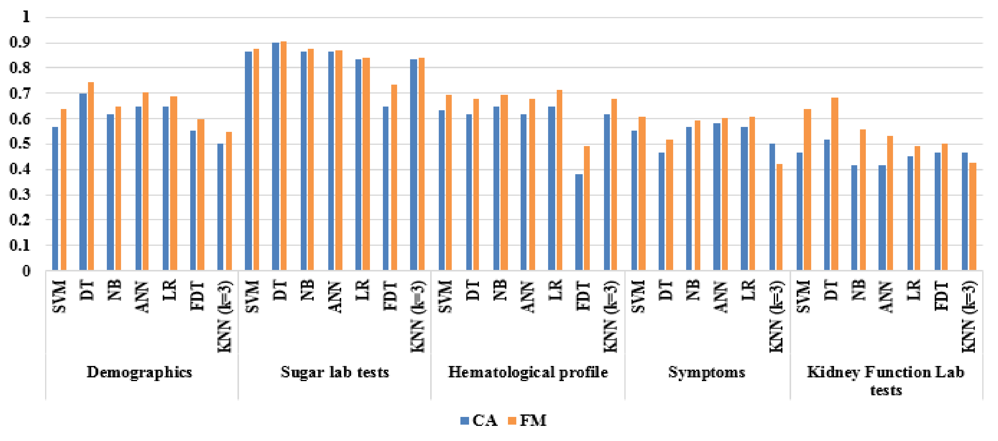
| Sub-Dataset | Algorithm | CA | Se | Sp | PPV | NPV | FM | MCC | FPR | FNR | ER | GM |
|---|---|---|---|---|---|---|---|---|---|---|---|---|
| Demographics | SVM | 0.567 | 0.719 | 0.393 | 0.575 | 0.550 | 0.639 | 0.118 | 0.607 | 0.281 | 0.433 | 1.054 |
| DT | 0.700 | 0.813 | 0.571 | 0.684 | 0.727 | 0.743 | 0.397 | 0.429 | 0.188 | 0.300 | 1.177 | |
| NB | 0.616 | 0.656 | 0.571 | 0.636 | 0.593 | 0.646 | 0.228 | 0.429 | 0.344 | 0.384 | 1.108 | |
| ANN | 0.650 | 0.781 | 0.500 | 0.641 | 0.667 | 0.704 | 0.294 | 0.500 | 0.219 | 0.350 | 1.132 | |
| LR | 0.650 | 0.719 | 0.571 | 0.657 | 0.640 | 0.687 | 0.294 | 0.429 | 0.281 | 0.350 | 1.136 | |
| FDT | 0.550 | 0.625 | 0.464 | 0.571 | 0.520 | 0.597 | 0.090 | 0.536 | 0.375 | 0.450 | 1.044 | |
| KNN (k = 3) | 0.500 | 0.563 | 0.429 | 0.529 | 0.462 | 0.545 | 0.009 | 0.571 | 0.438 | 0.500 | 0.996 | |
| Sugar lab tests | SVM | 0.867 | 0.875 | 0.857 | 0.875 | 0.857 | 0.875 | 0.732 | 0.143 | 0.125 | 0.133 | 1.316 |
| DT | 0.900 | 0.906 | 0.893 | 0.906 | 0.893 | 0.906 | 0.799 | 0.107 | 0.094 | 0.100 | 1.341 | |
| NB | 0.867 | 0.875 | 0.857 | 0.875 | 0.857 | 0.875 | 0.732 | 0.143 | 0.125 | 0.133 | 1.316 | |
| ANN | 0.867 | 0.844 | 0.893 | 0.900 | 0.833 | 0.871 | 0.735 | 0.107 | 0.156 | 0.133 | 1.318 | |
| LR | 0.833 | 0.813 | 0.857 | 0.867 | 0.800 | 0.839 | 0.668 | 0.143 | 0.188 | 0.167 | 1.292 | |
| FDT | 0.648 | 0.963 | 0.333 | 0.591 | 0.900 | 0.732 | 0.381 | 0.667 | 0.037 | 0.352 | 1.139 | |
| KNN (k = 3) | 0.833 | 0.813 | 0.857 | 0.867 | 0.800 | 0.839 | 0.668 | 0.143 | 0.188 | 0.167 | 1.292 | |
| Hematological profiles | SVM | 0.633 | 0.781 | 0.464 | 0.625 | 0.650 | 0.694 | 0.260 | 0.536 | 0.219 | 0.367 | 1.116 |
| DT | 0.617 | 0.750 | 0.464 | 0.615 | 0.619 | 0.676 | 0.224 | 0.536 | 0.250 | 0.383 | 1.102 | |
| NB | 0.650 | 0.750 | 0.536 | 0.649 | 0.652 | 0.696 | 0.293 | 0.464 | 0.250 | 0.350 | 1.134 | |
| ANN | 0.617 | 0.750 | 0.464 | 0.615 | 0.619 | 0.676 | 0.224 | 0.536 | 0.250 | 0.383 | 1.102 | |
| LR | 0.650 | 0.813 | 0.464 | 0.634 | 0.684 | 0.712 | 0.297 | 0.536 | 0.188 | 0.350 | 1.130 | |
| FDT | 0.383 | 0.563 | 0.464 | 0.439 | 0.433 | 0.493 | 0.270 | 0.821 | 0.531 | 0.617 | 1.014 | |
| KNN (k = 3) | 0.617 | 0.750 | 0.464 | 0.615 | 0.619 | 0.676 | 0.224 | 0.536 | 0.250 | 0.383 | 1.102 | |
| Symptoms | SVM | 0.550 | 0.656 | 0.429 | 0.568 | 0.522 | 0.609 | 0.087 | 0.571 | 0.344 | 0.450 | 1.041 |
| DT | 0.467 | 0.531 | 0.393 | 0.500 | 0.423 | 0.515 | 0.076 | 0.607 | 0.469 | 0.533 | 0.961 | |
| NB | 0.567 | 0.594 | 0.536 | 0.594 | 0.536 | 0.594 | 0.129 | 0.464 | 0.406 | 0.433 | 1.063 | |
| ANN | 0.583 | 0.594 | 0.571 | 0.613 | 0.552 | 0.603 | 0.165 | 0.429 | 0.406 | 0.417 | 1.080 | |
| LR | 0.567 | 0.625 | 0.500 | 0.588 | 0.538 | 0.606 | 0.126 | 0.500 | 0.375 | 0.433 | 1.061 | |
| KNN (k = 3) | 0.500 | 0.344 | 0.679 | 0.550 | 0.475 | 0.423 | 0.024 | 0.321 | 0.656 | 0.500 | 1.011 | |
| Kidney function lab tests | SVM | 0.467 | 0.875 | 0.000 | 0.500 | 0.000 | 0.636 | 0.250 | 1.000 | 0.125 | 0.533 | 0.935 |
| DT | 0.517 | 0.969 | 0.000 | 0.525 | 0.000 | 0.681 | 0.122 | 1.000 | 0.031 | 0.483 | 0.984 | |
| NB | 0.417 | 0.688 | 0.107 | 0.468 | 0.231 | 0.557 | 0.249 | 0.893 | 0.313 | 0.583 | 0.892 | |
| ANN | 0.417 | 0.625 | 0.179 | 0.465 | 0.294 | 0.533 | 0.217 | 0.821 | 0.375 | 0.583 | 0.896 | |
| LR | 0.450 | 0.500 | 0.393 | 0.485 | 0.407 | 0.492 | 0.107 | 0.607 | 0.500 | 0.550 | 0.945 | |
| FDT | 0.467 | 0.500 | 0.429 | 0.500 | 0.429 | 0.500 | 0.071 | 0.571 | 0.500 | 0.533 | 0.964 | |
| KNN (k = 3) | 0.467 | 0.375 | 0.571 | 0.500 | 0.444 | 0.429 | 0.055 | 0.429 | 0.625 | 0.533 | 0.973 | |
| Lipid profiles | SVM | 0.500 | 0.875 | 0.071 | 0.519 | 0.333 | 0.651 | 0.089 | 0.929 | 0.125 | 0.500 | 0.973 |
| DT | 0.633 | 0.938 | 0.286 | 0.600 | 0.800 | 0.732 | 0.299 | 0.714 | 0.063 | 0.367 | 1.106 | |
| NB | 0.517 | 0.281 | 0.786 | 0.600 | 0.489 | 0.383 | 0.077 | 0.214 | 0.719 | 0.483 | 1.033 | |
| ANN | 0.567 | 0.844 | 0.250 | 0.563 | 0.583 | 0.675 | 0.117 | 0.750 | 0.156 | 0.433 | 1.046 | |
| LR | 0.517 | 0.719 | 0.286 | 0.535 | 0.471 | 0.613 | 0.005 | 0.714 | 0.281 | 0.483 | 1.002 | |
| FDT | 0.467 | 0.438 | 0.250 | 0.500 | 0.333 | 0.467 | 0.063 | 0.500 | 0.438 | 0.533 | 0.829 | |
| KNN (k = 3) | 0.567 | 0.875 | 0.214 | 0.560 | 0.600 | 0.683 | 0.120 | 0.786 | 0.125 | 0.433 | 1.044 | |
| Urine analysis | SVM | 0.667 | 0.500 | 0.857 | 0.800 | 0.600 | 0.615 | 0.378 | 0.143 | 0.500 | 0.333 | 1.165 |
| DT | 0.683 | 0.531 | 0.857 | 0.810 | 0.615 | 0.642 | 0.406 | 0.143 | 0.469 | 0.317 | 1.178 | |
| NB | 0.667 | 0.500 | 0.857 | 0.800 | 0.600 | 0.615 | 0.378 | 0.143 | 0.500 | 0.333 | 1.165 | |
| ANN | 0.700 | 0.500 | 0.929 | 0.889 | 0.619 | 0.640 | 0.467 | 0.071 | 0.500 | 0.300 | 1.195 | |
| LR | 0.667 | 0.469 | 0.893 | 0.833 | 0.595 | 0.600 | 0.394 | 0.107 | 0.531 | 0.333 | 1.167 | |
| KNN (k = 3) | 0.683 | 0.531 | 0.857 | 0.810 | 0.615 | 0.642 | 0.406 | 0.143 | 0.469 | 0.317 | 1.178 | |
| Liver function tests | SVM | 0.483 | 0.813 | 0.107 | 0.510 | 0.333 | 0.627 | 0.112 | 0.893 | 0.188 | 0.517 | 0.959 |
| DT | 0.417 | 0.594 | 0.214 | 0.463 | 0.316 | 0.521 | 0.206 | 0.786 | 0.406 | 0.583 | 0.899 | |
| NB | 0.533 | 0.250 | 0.857 | 0.667 | 0.500 | 0.364 | 0.134 | 0.143 | 0.750 | 0.467 | 1.052 | |
| ANN | 0.500 | 0.531 | 0.464 | 0.531 | 0.464 | 0.531 | 0.004 | 0.536 | 0.469 | 0.500 | 0.998 | |
| LR | 0.550 | 0.469 | 0.643 | 0.600 | 0.514 | 0.526 | 0.113 | 0.357 | 0.531 | 0.450 | 1.054 | |
| FDT | 0.617 | 0.375 | 0.405 | 0.800 | 0.556 | 0.511 | 0.309 | 0.107 | 0.625 | 0.383 | 0.883 | |
| KNN (k = 3) | 0.583 | 0.500 | 0.679 | 0.640 | 0.543 | 0.561 | 0.181 | 0.321 | 0.500 | 0.417 | 1.086 | |
| Diseases | SVM | 0.517 | 0.438 | 0.607 | 0.560 | 0.486 | 0.491 | 0.045 | 0.393 | 0.563 | 0.483 | 1.022 |
| DT | 0.450 | 0.375 | 0.536 | 0.480 | 0.429 | 0.421 | 0.090 | 0.464 | 0.625 | 0.550 | 0.954 | |
| NB | 0.600 | 0.500 | 0.714 | 0.667 | 0.556 | 0.571 | 0.218 | 0.286 | 0.500 | 0.400 | 1.102 | |
| ANN | 0.533 | 0.375 | 0.714 | 0.600 | 0.500 | 0.462 | 0.094 | 0.286 | 0.625 | 0.467 | 1.044 | |
| LR | 0.483 | 0.281 | 0.714 | 0.529 | 0.465 | 0.367 | 0.005 | 0.286 | 0.719 | 0.517 | 0.998 | |
| KNN | 0.466 | 0.344 | 0.607 | 0.500 | 0.447 | 0.407 | 0.051 | 0.393 | 0.656 | 0.534 | 0.975 |
| Dataset | Algorithm | CA | Se | Sp | PPV | NPV | FM | MCC | FPR | FNR | ER | GM |
|---|---|---|---|---|---|---|---|---|---|---|---|---|
| Demographics | SVM | 0.700 | 0.813 | 0.571 | 0.684 | 0.727 | 0.743 | 0.397 | 0.429 | 0.188 | 0.300 | 1.177 |
| DT | 0.667 | 0.906 | 0.393 | 0.630 | 0.786 | 0.744 | 0.353 | 0.607 | 0.094 | 0.333 | 1.140 | |
| NB | 0.650 | 0.688 | 0.607 | 0.667 | 0.630 | 0.677 | 0.295 | 0.393 | 0.313 | 0.350 | 1.138 | |
| ANN | 0.700 | 0.813 | 0.571 | 0.684 | 0.727 | 0.743 | 0.397 | 0.429 | 0.188 | 0.300 | 1.177 | |
| LR | 0.633 | 0.688 | 0.571 | 0.647 | 0.615 | 0.667 | 0.261 | 0.429 | 0.313 | 0.367 | 1.122 | |
| FDT | 0.483 | 0.625 | 0.321 | 0.513 | 0.429 | 0.563 | 0.056 | 0.679 | 0.375 | 0.517 | 0.973 | |
| KNN (k = 3) | 0.650 | 0.656 | 0.643 | 0.677 | 0.621 | 0.667 | 0.299 | 0.357 | 0.344 | 0.350 | 1.140 | |
| Sugar lab tests | SVM | 0.867 | 0.875 | 0.857 | 0.875 | 0.857 | 0.875 | 0.732 | 0.143 | 0.125 | 0.133 | 1.316 |
| DT | 0.900 | 0.906 | 0.893 | 0.906 | 0.893 | 0.906 | 0.799 | 0.107 | 0.094 | 0.100 | 1.341 | |
| NB | 0.883 | 0.875 | 0.893 | 0.903 | 0.862 | 0.889 | 0.767 | 0.107 | 0.125 | 0.117 | 1.330 | |
| ANN | 0.883 | 0.875 | 0.643 | 0.903 | 0.621 | 0.889 | 0.767 | 0.107 | 0.344 | 0.117 | 1.232 | |
| LR | 0.850 | 0.844 | 0.857 | 0.871 | 0.828 | 0.857 | 0.700 | 0.143 | 0.156 | 0.150 | 1.304 | |
| FDT | 0.648 | 0.963 | 0.333 | 0.591 | 0.900 | 0.732 | 0.381 | 0.667 | 0.037 | 0.352 | 1.139 | |
| KNN (k = 3) | 0.867 | 0.844 | 0.893 | 0.900 | 0.833 | 0.871 | 0.735 | 0.107 | 0.156 | 0.133 | 1.318 | |
| Hematological profiles | SVM | 0.600 | 0.781 | 0.393 | 0.595 | 0.611 | 0.676 | 0.190 | 0.607 | 0.219 | 0.400 | 1.083 |
| DT | 0.567 | 0.719 | 0.393 | 0.575 | 0.550 | 0.639 | 0.118 | 0.607 | 0.281 | 0.433 | 1.054 | |
| NB | 0.667 | 0.750 | 0.571 | 0.667 | 0.667 | 0.706 | 0.327 | 0.429 | 0.250 | 0.333 | 1.150 | |
| ANN | 0.650 | 0.750 | 0.536 | 0.649 | 0.652 | 0.696 | 0.293 | 0.464 | 0.250 | 0.350 | 1.134 | |
| LR | 0.633 | 0.813 | 0.429 | 0.619 | 0.667 | 0.703 | 0.262 | 0.571 | 0.188 | 0.357 | 1.114 | |
| FDT | 0.417 | 0.594 | 0.214 | 0.463 | 0.316 | 0.521 | 0.206 | 0.786 | 0.406 | 0.583 | 0.899 | |
| KNN (k = 3) | 0.583 | 0.625 | 0.536 | 0.606 | 0.556 | 0.615 | 0.161 | 0.464 | 0.375 | 0.417 | 1.077 | |
| Symptoms | SVM | 0.617 | 0.469 | 0.786 | 0.714 | 0.564 | 0.566 | 0.266 | 0.214 | 0.531 | 0.383 | 1.120 |
| DT | 0.467 | 0.375 | 0.571 | 0.500 | 0.444 | 0.429 | 0.055 | 0.429 | 0.625 | 0.533 | 0.973 | |
| NB | 0.550 | 0.563 | 0.536 | 0.581 | 0.517 | 0.571 | 0.098 | 0.464 | 0.438 | 0.450 | 1.048 | |
| ANN | 0.467 | 0.375 | 0.571 | 0.500 | 0.444 | 0.429 | 0.055 | 0.429 | 0.625 | 0.533 | 0.973 | |
| LR | 0.550 | 0.625 | 0.464 | 0.571 | 0.520 | 0.597 | 0.090 | 0.536 | 0.375 | 0.450 | 1.044 | |
| KNN (k = 3) | 0.500 | 0.563 | 0.429 | 0.529 | 0.462 | 0.545 | 0.009 | 0.571 | 0.438 | 0.500 | 0.996 | |
| Kidney function lab tests | SVM | 0.500 | 0.875 | 0.071 | 0.519 | 0.333 | 0.651 | 0.089 | 0.929 | 0.125 | 0.500 | 0.973 |
| DT | 0.533 | 1.000 | 0.000 | 0.533 | 0.000 | 0.696 | 0.000 | 1.000 | 0.000 | 0.467 | 1.000 | |
| NB | 0.433 | 0.531 | 0.321 | 0.472 | 0.375 | 0.500 | 0.150 | 0.679 | 0.469 | 0.567 | 0.923 | |
| ANN | 0.450 | 0.625 | 0.447 | 0.488 | 0.586 | 0.548 | 0.134 | 0.750 | 0.375 | 0.550 | 1.036 | |
| LR | 0.417 | 0.531 | 0.286 | 0.459 | 0.348 | 0.493 | 0.188 | 0.714 | 0.469 | 0.583 | 0.904 | |
| FDT | 0.467 | 0.594 | 0.321 | 0.500 | 0.409 | 0.543 | 0.088 | 0.679 | 0.406 | 0.533 | 0.957 | |
| KNN (k = 3) | 0.533 | 0.469 | 0.607 | 0.577 | 0.500 | 0.517 | 0.076 | 0.393 | 0.531 | 0.467 | 1.037 | |
| Lipid profiles | SVM | 0.533 | 1.000 | 0.000 | 0.533 | DIV/0! | 0.696 | 0.000 | 1.000 | 0.000 | 0.457 | 1.000 |
| DT | 0.600 | 0.938 | 0.214 | 0.577 | 0.750 | 0.714 | 0.223 | 0.786 | 0.063 | 0.400 | 1.073 | |
| NB | 0.517 | 0.375 | 0.321 | 0.571 | 0.310 | 0.453 | 0.056 | 0.321 | 0.625 | 0.483 | 0.835 | |
| ANN | 0.667 | 0.906 | 0.393 | 0.630 | 0.786 | 0.744 | 0.353 | 0.607 | 0.094 | 0.333 | 1.140 | |
| LR | 0.617 | 0.719 | 0.500 | 0.622 | 0.609 | 0.667 | 0.224 | 0.500 | 0.281 | 0.383 | 1.104 | |
| FDT | 0.483 | 0.531 | 0.429 | 0.515 | 0.444 | 0.523 | 0.040 | 0.571 | 0.469 | 0.517 | 0.980 | |
| KNN (k = 3) | 0.600 | 0.594 | 0.607 | 0.633 | 0.567 | 0.613 | 0.200 | 0.393 | 0.406 | 0.400 | 1.096 | |
| Urine analysis | SVM | 0.717 | 0.469 | 1.000 | 1.000 | 0.622 | 0.638 | 0.540 | 0.000 | 0.531 | 0.283 | 1.212 |
| DT | 0.683 | 0.531 | 0.857 | 0.810 | 0.615 | 0.642 | 0.406 | 0.143 | 0.469 | 0.317 | 1.178 | |
| NB | 0.650 | 0.500 | 0.821 | 0.762 | 0.590 | 0.604 | 0.336 | 0.179 | 0.500 | 0.350 | 1.150 | |
| ANN | 0.717 | 0.500 | 0.964 | 0.941 | 0.628 | 0.653 | 0.514 | 0.036 | 0.500 | 0.283 | 1.210 | |
| LR | 0.733 | 0.500 | 1.000 | 1.000 | 0.636 | 0.667 | 0.564 | 0.000 | 0.500 | 0.267 | 1.225 | |
| KNN (k = 3) | 0.683 | 0.438 | 0.964 | 0.933 | 0.600 | 0.596 | 0.463 | 0.036 | 0.563 | 0.317 | 1.184 | |
| Liver function tests | SVM | 0.417 | 0.625 | 0.179 | 0.465 | 0.294 | 0.533 | 0.217 | 0.821 | 0.375 | 0.583 | 0.896 |
| DT | 0.450 | 0.656 | 0.214 | 0.488 | 0.353 | 0.560 | 0.143 | 0.786 | 0.344 | 0.550 | 0.933 | |
| NB | 0.483 | 0.250 | 0.750 | 0.533 | 0.467 | 0.340 | 0.000 | 0.250 | 0.750 | 0.517 | 1.000 | |
| ANN | 0.617 | 0.500 | 0.391 | 0.696 | 0.568 | 0.582 | 0.257 | 0.250 | 0.500 | 0.383 | 0.944 | |
| LR | 0.500 | 0.625 | 0.357 | 0.526 | 0.455 | 0.571 | 0.018 | 0.643 | 0.375 | 0.500 | 0.991 | |
| FDT | 0.650 | 0.438 | 0.893 | 0.824 | 0.581 | 0.571 | 0.366 | 0.107 | 0.563 | 0.350 | 1.154 | |
| KNN (k = 3) | 0.617 | 0.688 | 0.536 | 0.629 | 0.600 | 0.657 | 0.226 | 0.464 | 0.313 | 0.383 | 1.106 | |
| Diseases | SVM | 0.657 | 0.313 | 0.857 | 0.714 | 0.522 | 0.435 | 0.200 | 0.143 | 0.688 | 0.433 | 1.082 |
| DT | 0.483 | 0.375 | 0.607 | 0.522 | 0.459 | 0.436 | 0.018 | 0.393 | 0.625 | 0.517 | 0.991 | |
| NB | 0.600 | 0.500 | 0.714 | 0.667 | 0.556 | 0.571 | 0.218 | 0.286 | 0.500 | 0.400 | 1.102 | |
| ANN | 0.567 | 0.406 | 0.750 | 0.650 | 0.525 | 0.500 | 0.165 | 0.250 | 0.594 | 0.433 | 1.075 | |
| LR | 0.533 | 0.406 | 0.679 | 0.591 | 0.500 | 0.481 | 0.088 | 0.321 | 0.594 | 0.467 | 1.041 | |
| KNN (k = 3) | 0.517 | 0.469 | 0.571 | 0.556 | 0.485 | 0.508 | 0.040 | 0.429 | 0.531 | 0.483 | 1.020 |
| No. | Dataset | Base Algorithm | FS Technique | Weight (FM) |
|---|---|---|---|---|
| 1 | Demographics | SVM | Wrapper | 74.4 |
| 2 | Sugar lab tests | DT | Correlation FS | 90.6 |
| 3 | Hematological profiles | LR | Correlation FS | 71.2 |
| 4 | Symptoms | ANN | Correlation FS | 60.3 |
| 5 | Kidney function Lab tests | DT | Wrapper | 69.6 |
| 6 | Lipid profile | ANN | Wrapper | 66.7 |
| 7 | Urine analysis | LR | Wrapper | 74.4 |
| 8 | Liver function tests | FDT | Wrapper | 57.1 |
| 9 | Diseases | ANN | Correlation FS | 46.2 |
| Sub-Dataset | Algorithm | CA | Se | Sp | PPV | NPV | FM | MCC | FPR | FNR | ER | GM |
|---|---|---|---|---|---|---|---|---|---|---|---|---|
| Demographics | RF | 0.617 | 0.719 | 0.500 | 0.622 | 0.609 | 0.667 | 0.224 | 0.500 | 0.281 | 0.383 | 1.104 |
| Bagging | 0.667 | 0.781 | 0.536 | 0.658 | 0.682 | 0.714 | 0.328 | 0.464 | 0.219 | 0.333 | 1.147 | |
| Voting | 0.650 | 0.688 | 0.607 | 0.667 | 0.630 | 0.677 | 0.295 | 0.393 | 0.313 | 0.530 | 1.138 | |
| Stacking | 0.567 | 0.500 | 0.643 | 0.615 | 0.529 | 0.552 | 0.144 | 0.357 | 0.500 | 0.433 | 1.069 | |
| AdaBoostM1 | 0.700 | 0.781 | 0.607 | 0.694 | 0.708 | 0.735 | 0.396 | 0.393 | 0.219 | 0.300 | 1.178 | |
| Sugar lab tests | RF | 0.867 | 0.844 | 0.893 | 0.900 | 0.833 | 0.871 | 0.735 | 0.107 | 0.156 | 0.133 | 1.318 |
| Bagging | 0.867 | 0.875 | 0.857 | 0.875 | 0.857 | 0.875 | 0.732 | 0.143 | 0.125 | 0.133 | 1.316 | |
| Voting | 0.867 | 0.875 | 0.857 | 0.875 | 0.857 | 0.875 | 0.732 | 0.143 | 0.125 | 0.133 | 1.316 | |
| Stacking | 0.850 | 0.844 | 0.857 | 0.871 | 0.828 | 0.857 | 0.700 | 0.143 | 0.156 | 0.150 | 1.304 | |
| AdaBoostM1 | 0.867 | 0.844 | 0.893 | 0.900 | 0.833 | 0.871 | 0.735 | 0.107 | 0.156 | 0.133 | 1.318 | |
| Hematological profiles | RF | 0.617 | 0.750 | 0.464 | 0.615 | 0.619 | 0.676 | 0.224 | 0.536 | 0.250 | 0.383 | 1.102 |
| Bagging | 0.633 | 0.750 | 0.500 | 0.632 | 0.636 | 0.686 | 0.259 | 0.500 | 0.250 | 0.367 | 1.118 | |
| Voting | 0.617 | 0.750 | 0.464 | 0.615 | 0.619 | 0.676 | 0.224 | 0.536 | 0.250 | 0.383 | 1.102 | |
| Stacking | 0.533 | 0.563 | 0.500 | 0.563 | 0.500 | 0.563 | 0.063 | 0.500 | 0.438 | 0.467 | 1.031 | |
| AdaBoostM1 | 0.650 | 0.813 | 0.464 | 0.634 | 0.684 | 0.712 | 0.297 | 0.536 | 0.188 | 0.350 | 1.130 | |
| Symptoms | RF | 0.567 | 0.531 | 0.607 | 0.607 | 0.531 | 0.567 | 0.138 | 0.393 | 0.469 | 0.433 | 1.067 |
| Bagging | 0.500 | 0.563 | 0.429 | 0.529 | 0.462 | 0.545 | 0.009 | 0.571 | 0.438 | 0.500 | 0.996 | |
| Voting | 0.517 | 0.531 | 0.500 | 0.548 | 0.483 | 0.540 | 0.031 | 0.500 | 0.469 | 0.483 | 1.015 | |
| Stacking | 0.467 | 0.563 | 0.357 | 0.500 | 0.417 | 0.529 | 0.082 | 0.643 | 0.438 | 0.533 | 0.959 | |
| AdaBoostM1 | 0.533 | 0.594 | 0.464 | 0.559 | 0.500 | 0.576 | 0.058 | 0.536 | 0.406 | 0.467 | 1.029 | |
| Kidney function lab tests | RF | 0.400 | 0.344 | 0.464 | 0.423 | 0.382 | 0.379 | 0.193 | 0.536 | 0.656 | 0.600 | 0.899 |
| Bagging | 0.417 | 0.563 | 0.250 | 0.462 | 0.333 | 0.507 | 0.196 | 0.750 | 0.438 | 0.583 | 0.902 | |
| Voting | 0.483 | 0.906 | 0.000 | 0.509 | 0.000 | 0.652 | 0.215 | 1.000 | 0.094 | 0.517 | 0.952 | |
| Stacking | 0.550 | 0.750 | 0.321 | 0.558 | 0.529 | 0.640 | 0.079 | 0.679 | 0.250 | 0.450 | 1.035 | |
| AdaBoostM1 | 0.517 | 0.969 | 0.000 | 0.525 | 0.000 | 0.681 | 0.122 | 1.000 | 0.031 | 0.483 | 0.984 | |
| Lipid profiles | RF | 0.650 | 0.906 | 0.357 | 0.617 | 0.769 | 0.734 | 0.319 | 0.643 | 0.094 | 0.350 | 1.124 |
| Bagging | 0.533 | 0.750 | 0.286 | 0.545 | 0.500 | 0.632 | 0.040 | 0.714 | 0.250 | 0.467 | 1.018 | |
| Voting | 0.600 | 0.875 | 0.286 | 0.583 | 0.667 | 0.700 | 0.200 | 0.714 | 0.125 | 0.400 | 1.077 | |
| Stacking | 0.583 | 0.781 | 0.357 | 0.581 | 0.588 | 0.667 | 0.153 | 0.643 | 0.219 | 0.417 | 1.067 | |
| AdaBoostM1 | 0.633 | 0.969 | 0.250 | 0.596 | 0.875 | 0.738 | 0.321 | 0.750 | 0.031 | 0.367 | 1.104 | |
| Urine analysis | RF | 0.667 | 0.500 | 0.857 | 0.800 | 0.600 | 0.615 | 0.378 | 0.143 | 0.500 | 0.333 | 1.165 |
| Bagging | 0.667 | 0.500 | 0.857 | 0.800 | 0.600 | 0.615 | 0.378 | 0.143 | 0.500 | 0.333 | 1.165 | |
| Voting | 0.683 | 0.531 | 0.857 | 0.810 | 0.615 | 0.642 | 0.406 | 0.143 | 0.469 | 0.317 | 1.178 | |
| Stacking | 0.583 | 0.406 | 0.786 | 0.684 | 0.537 | 0.510 | 0.206 | 0.214 | 0.594 | 0.417 | 1.092 | |
| AdaBoostM1 | 0.667 | 0.500 | 0.857 | 0.800 | 0.600 | 0.615 | 0.378 | 0.143 | 0.500 | 0.333 | 1.165 | |
| Liver function tests | RF | 0.500 | 0.500 | 0.500 | 0.533 | 0.467 | 0.516 | 0.000 | 0.500 | 0.500 | 0.500 | 1.000 |
| Bagging | 0.533 | 0.250 | 0.857 | 0.667 | 0.500 | 0.364 | 0.134 | 0.143 | 0.750 | 0.467 | 1.052 | |
| Voting | 0.550 | 0.438 | 0.679 | 0.609 | 0.514 | 0.509 | 0.119 | 0.321 | 0.563 | 0.450 | 1.057 | |
| Stacking | 0.517 | 0.531 | 0.500 | 0.548 | 0.483 | 0.540 | 0.031 | 0.500 | 0.469 | 0.483 | 1.015 | |
| AdaBoostM1 | 0.533 | 0.250 | 0.857 | 0.667 | 0.500 | 0.364 | 0.134 | 0.143 | 0.750 | 0.467 | 1.052 | |
| Diseases | RF | 0.500 | 0.406 | 0.607 | 0.542 | 0.472 | 0.464 | 0.014 | 0.393 | 0.594 | 0.500 | 1.007 |
| Bagging | 0.533 | 0.531 | 0.536 | 0.567 | 0.500 | 0.548 | 0.067 | 0.464 | 0.469 | 0.467 | 1.033 | |
| Voting | 0.550 | 0.406 | 0.714 | 0.619 | 0.513 | 0.491 | 0.126 | 0.286 | 0.594 | 0.450 | 1.058 | |
| Stacking | 0.483 | 0.500 | 0.464 | 0.516 | 0.448 | 0.508 | 0.036 | 0.536 | 0.500 | 0.517 | 0.982 | |
| AdaBoostM1 | 0.600 | 0.500 | 0.714 | 0.667 | 0.556 | 0.571 | 0.218 | 0.286 | 0.500 | 0.400 | 1.102 |
© 2019 by the authors. Licensee MDPI, Basel, Switzerland. This article is an open access article distributed under the terms and conditions of the Creative Commons Attribution (CC BY) license (http://creativecommons.org/licenses/by/4.0/).
Share and Cite
El-Sappagh, S.; Elmogy, M.; Ali, F.; ABUHMED, T.; Islam, S.M.R.; Kwak, K.-S. A Comprehensive Medical Decision–Support Framework Based on a Heterogeneous Ensemble Classifier for Diabetes Prediction. Electronics 2019, 8, 635. https://doi.org/10.3390/electronics8060635
El-Sappagh S, Elmogy M, Ali F, ABUHMED T, Islam SMR, Kwak K-S. A Comprehensive Medical Decision–Support Framework Based on a Heterogeneous Ensemble Classifier for Diabetes Prediction. Electronics. 2019; 8(6):635. https://doi.org/10.3390/electronics8060635
Chicago/Turabian StyleEl-Sappagh, Shaker, Mohammed Elmogy, Farman Ali, Tamer ABUHMED, S. M. Riazul Islam, and Kyung-Sup Kwak. 2019. "A Comprehensive Medical Decision–Support Framework Based on a Heterogeneous Ensemble Classifier for Diabetes Prediction" Electronics 8, no. 6: 635. https://doi.org/10.3390/electronics8060635