Impact of Component Dispersion in DC to DC Low-Power Low-Voltage Power Converter Array

Abstract

The paper deals with arrays of numerous power conversion cells, associated in series and/or in parallel to build larger step up or step down direct current (DC)/DC isolated converters. The work focuses on the impact of the spread and distribution of the conversion cell characteristics on the characteristics and performance of the power converter array (PCA). Based on a characterization protocol, about 130 conversion standard cells (CSC) are characterized and classified from a statistical point of view. Three families are defined and representatives are chosen and implemented in various configurations, in open and closed loop control, to analyze the impact of their spread characteristic over the global converter, the PCA. The paper is based on an extended practical set up and protocols, all described in details. Guidelines on CSCs implementation with respect to their dispersion are provided at the end on the paper.

1. Introduction

Power electronics converters arrays are gaining more interest because of their multiple advantages thanks to voltage and current ratings distribution over several conversion cells [1,2]. Basically, a power converter array (PCA) is built from the association in series or in parallel of several converter cells, allowing to scale up voltage and/or current ratings, to distribute voltage, current and losses over several conversion subsystems, but also to interleave control and filtering [3]. PCAs are different from the inter-cell of multi-level converters such as in [4,5,6] in the way the conversion cells remain far more independent. In addition, matrices of converters bring the opportunity to use standardized subsystems such as in power electronics building blocs (PEBB) [7,8]. Most of the time converter arrays, also called multi-cell converters, are made from a few conversion cell units. Power converter arrays can also be made from numerous conversion subsystems, for example with tens of conversion cells [9]. In such a way, complexity rises and standardization, together with integration (monolithic and hybrid), are used to overcome reliability issues [10]. Integration is used to increase reliability by relying on advanced and collective manufacturing platforms. In such a way, monolithic integration can be used to aggregate all active parts, including if possible, power transistors in a single device to reduce interconnects and assembly issues [11]. Hybrid integration is considered for the assembly of heterogeneous components in conversion sub modules such as Integrated Power Electronics Modules (IPEM) [12] for the same benefits. Both solutions are offering standardized and reliable parts that may balance converter complexity. For this, conversion standard cells (CSCs) are designed, produced and qualified to be used several times afterwards in many different PCAs, with the objective not to modify them. In such a way, higher yield is obtained, the supply chain may be optimized and the design cycle can be reduced as presented in [13,14]. Nonetheless, CSCs remain to be produced in quantities and tolerances on components and manufacturing process will keep introducing a spread in characteristics and performances at the CSC level. These characteristic and performance dispersions may as well affect voltage and/or current distribution over the PCA, leading to uneven distribution losses and possibly poor performance levels as for example in the case of photovoltaic (PV) panels [15]. To overcome this, extensive control is usually implemented leading to extra complexity and cost. The main objective of the paper is to investigate, on a precise case study, first the distribution of the characteristics at CSC level and then how this propagates to the PCA level. This paper does not aim to produce a generic analysis. It aims to introduce a qualification procedure. It is carried out on a specific technology frame and does not pretend the analysis can be fully transferred to any other case study.

In such a way, the paper is based on existing CSCs that are first characterized. A large set of devices are tested and classified before being implemented in PCAs in various configurations. From the whole analysis, it is expected to see which conditions may be necessary and how to handle the thermal management of CSC that are not fully operated at the same operating point. The whole analysis only considers a steady state operation. The impact of CSC characteristics spread in PCA dynamic responses to a reference step or input voltage variation or load step or any other operating point variation is not studied in this paper [16].

The paper describes first the CSC under study and its electrical characteristics. Then the paper focuses on the characterization of an industrial batch of CSCs to point out the fact that although they are all manufactured in the same batch (same architecture, same components from the same supply chain …), they exhibit differences in operation. In particular, the CSCs are classified and a relation is defined between CSCs characteristics and the critical components involved in the dispersion of CSCs. Out of a production batch of 250 CSCs, about 130 are tested in specific conditions and statistics are provided. Representative samples are extensively characterized before being used and implemented in multiple PCA configurations.

For that, three CSC families are defined and used to build several configurations in order to observe the impact of CSC dispersion on the characteristics and performance of PCA. A design of experiment (DOE) is proposed. Only open loop control is considered at this stage of the study. In such a way, the paper only provides an analysis that is suitable for steady state operation when PCAs are operated in a closed loop. As a consequence the paper is not addressing the impact of component dispersion on dynamic responses to disturbance or reference change when the PCA is working in closed loop. This is left to another study. The impact on voltage and current distribution is analyzed carefully, together with loss distribution and global efficiency. The paper ends with a set of guidelines in terms of CSC dispersion.

2. Setting up the Experiment

The work is based on arrays of standardized conversion cells that are associated at their input and output either in series or in parallel [17]. In such a way, almost any active transformation ratio can be achieved using the same CSC. CSCs integrate a decoupling between input and output terminals, a magnetic HF transformer in our case, such that any ISOP, IPOS and ISOS (respectively input series/output parallel, input parallel/output series and input series/output series) configuration can be implemented as illustrated in the Figure 1a [13]. The produced PCA can be made out of numerous CSCs, arranged in one configuration to form groups, the groups being able to be associated in the same or another configuration and so forth and so on until the global PCA meets the specification of the application. In this PCA design process, the only parameters that can be adjusted are the number of CSCs and the way they are interconnected in the PCA to fulfill specifications. The CSCs cannot be modified or adapted in order to maintain their yield high and to minimize rework at CSC levels. In our technology frame, CSC are assembled on a motherboard on which are implemented the power interconnections according to the desired configuration. Only motherboards are “customized” to receive power jumpers from one design to another. In such a way, step up or step down PCA with a large transformation ratio can be implemented and also voltage and current scaling is possible. In most cases, literature reports that control techniques are required in some configurations to account for CSCs voltage, current or power flow unbalances [18] CSCs considered in this work are all the same. They are DC to DC isolated converters based on a dual active bridge (DAB) topology, recalled in Figure 1b. Only this single architecture is studied in this paper. Each CSC includes all power devices, transistors, transformers, inductors and capacitors but also the gate drivers and the auxiliary supplies. Characteristics of a CSC are listed in

Table 1. Main characteristics of a single CSC and the PCA introduced as an illustration.

	Configuration	Input Voltage	Input Current	Output Voltage	Output Current	Power	Weight	Volume
Single CSC	Single	20 V	5 A	20 V	5 A	100 W	19 g	0.015 L
PCA	IPOS	20 V	90 A	320 V	5 A	1.8 kW	490 g	0.91 L

. MOSFETs are used in each H bridge and a HF transformer with unity transformation ratio is used, together with an AC link inductor. The two H bridges are switching at the same f_sw frequency with 0.5 duty cycle to produce AC square waveforms. The two AC waveforms are phase shifted of $\alpha$ to control power flow. Capacitors are placed on both sides of the HF transformer, in the AC link loop, to block the DC part of the not purely AC waved voltage by the full bridge. Otherwise, a DC voltage would be applied that would lead to the HF transformer magnetizing inductance saturation. Opto-couplers are also included on both sides of the DAB converter to receive the control signals for each H bridge. No specific control is implemented at the CSC level. In such a converter, power flow is very sensitive to AC link component values as shown in Equation (1). Especially, the AC link inductor value is a critical parameter in the Equation (1) where P_transferred is the power flow level from primary side to secondary side, V_in and V_out are respectively, the input and output DC bus voltages, L_AC is the AC link inductor, f_sw is the switching frequency and α is the phase shift angle between the primary side H bridge produced AC waveform and the secondary-side H bridge produced by the AC waveform. This makes the DAB converter a very suitable case study to investigate the impact of CSC component dispersion on PCA characteristics and performance.

$$P_{transferred}=\frac{V_{in}\ast V_{out}}{L_{AC}\ast f_{sw}}\alpha \left(1-2\alpha \right)$$

(1)

Step up or step down PCA can be built from associations of several or even numerous CSCs to achieve a very large active transformation ratio. In Figure 2 below are shown a picture of three CSCs and a picture of a PCA, made with 16 CSCs associated in an IPOS configuration, distributed in columns (×4), lines (×2) and boards (×2). It can be seen that two mother boards receive the CSC and a third PCB is used to complete the PCA configuration, collecting currents of paralleled CSC inputs and associating groups of CSCs in series at their outputs. The characteristics of the CSCs used in this work and the PCA presented as an illustration are summarized in Table 1 below. As can be seen in the picture, CSCs are physically stand-alone subsystems, manufactured on their own PCB. The implementation of the PCA is carried out with a mother board on which are soldered and interconnected CSCs. Termination standard cells are added on the edges of lines and columns of the array of CSCs in order to collect current and to implement the desired configuration. The PCA is designed to operate at full current of 5A under forced air cooling and down to half load under natural cooling. Since the whole characterization work is carried out under natural cooling test conditions, power flow will be limited. This implementation approach is very convenient for rapid prototyping where only mother boards are adapted from one PCA specification to another. In such a way, many CSCs can be produced at once and then implemented in various configurations.

This CSC has been designed exclusively with components available off the shelf, with regular dispersion constraints. The CSC has been optimized at best, with the objective to reach reasonable efficiency and power density levels, in order to be representative of a real design case. No component selection has been made prior to manufacturing to remove the one too far from the median characteristics.

Table 2. DAB converter component list. Includes the main value for the components and their dispersion range, when available.

Component	Value	Fonction	Main Parameter	Tolerance (%)
Transformer	POE120PL-24|300 nH leakage inductor	Galvanic Insulation	Ll	‘Maximum Value’
Inductors	XEL4030-301MEC|400 nH inductor	Alternating current (AC) link complement inductor	LAC	+/−20
Capacitor	20 µF 20 V	AC link decoupling capacitor	C	+/−20
Capacitor	20 µF 30 V	Input/Output filter capacitor	C	+/−20
MOSFET	SiSA10DN 5 mΩ 30 V	Power transistors	RDSon	+20

summarizes the main components to be used, together with their main characteristics and their known dispersion, when available, coming from datasheet.

The most representative characteristic curves of the DAB converter are the relation between efficiency and current rating (i.e., power level) and the relation between efficiency and the input, output voltage difference. Both of them have been plotted for the CSC that has been described and are provided as an example for one of them in Figure 3. As can be seen, the DAB converter efficiency is greatly affected by these two parameters. From these characterizations, one can easily understand that CSC dispersion may rapidly introduce operating point dispersion leading to performance dispersion. The important issue is then to see how dispersion levels are going to affect PCA converter performances. The following section introduces the characterization method used to qualify about 130 CSCs out of 250 devices manufactured from the same batch. Characterization results are then displayed and samples are selected to further analyze the distribution impact of CSCs when implemented in PCA.

3. Characterization of First Batch of Conversion Standard Cells (CSCs)

A test bench has been specifically developed in order to be able to implement fast and reproducible tests. The results are summarized in a graphical form to ease analysis. From that, three families of three CSCs are selected and further characterized and analyzed. This section details these steps.

3.1. Experimental Setup

CSCs have been designed to be assembled and interconnected on motherboards as presented in the previous section. This approach is very convenient for rapid prototyping. In addition, this is also very convenient for rapid testing and characterization on a socket board. A specific board has been designed to carry out the CSCs testing and characterization. Figure 4 below presents a picture of the PCB-based test board used for characterization, together with all the instrumentation required. In this test board, CSCs are not soldered as it is the case with the PCA shown in Figure 2. They are installed in a specific socket arrangement. Only natural air cooling can be implemented in a reproducible way. As a result CSCs will only be tested at up to half power. Since the socket may introduce additional resistance, a kelvin point measurement is implemented in order to measure accurately the input voltage applied to the CSCs and its output voltage without including the possible voltage drops that the sockets electrodes may add. Input and output voltage and currents are measured. Each CSC is supplied with the same DC source and strictly under the same voltage rating. The CSCs are loaded with a resistor that is strictly kept constant. The CSCs are controlled with a microcontroller that produces strictly the same switching frequency and the same phase shift between primary and secondary side driving signals.

Three different operating conditions were tested and are listed in

Table 3. Description of the three operating points used to characterize each single CSC.

Operation Point	Output Voltage (Considering 15Vinput)	Power Rating
N° 1	13 V	20 W
N° 2	14.5 V	20 W
N° 3	14.5 V	40 W

below. These testing conditions have been selected when CSC characteristics are either very sensitive or in the opposite way when they are not. This sensitivity is visible in the efficiency and electrical operating point in the curves in Figure 3. Specifically it can be seen that with a V_out/V_in ratio lower than 0.95 the efficiency becomes significantly sensitive to variations of V_out/V_in. The same conclusion can be drawn for power.

Three different points were considered to cover all operating regions. Operating point 1 considers a large input output voltage difference (large sensitivity) under a low power rating (large sensitivity). In this operating point, the efficiency level is very sensitive to power flow or voltage difference as can be seen in Figure 3. Similarly, operating point 2 considers a low input output voltage difference (low sensitivity) under a low power rating (large sensitivity). Operating point 3 considers a low input output voltage difference (low sensitivity) under 40 W power rating (low sensitivity). Of course more and/or different operating points could have been selected but this would have enlarged testing duration since the 130 CSCs are all tested for those three operating points. Especially a last operating point could have been selected at maximum power. This has not been implemented because it requires forced air cooling and the test bench was not implemented at first to operate under forced air cooled in a reproducible way. That characterization is left for complementary investigation.

From this characterization procedure, two parameters were specifically observed: the output voltage mismatch among cells and the CSCs efficiency mismatch. These two parameters were selected because they are very relevant of the converter operating point as a function of components values and parasitics. Especially, as introduced above in Equation (1), the AC link inductor has a significant impact on the converter operating point.

3.2. Characterization Results and First Analysis

Figure 5a below presents the distributions of the output voltage levels for over 130 tested CSCs under the conditions described in Table 3. The measured voltages are, therefore, close to the desired voltage in Table 3: the difference is due to the disparity in the value of the components. It is possible to represent the distribution of each test by normalizing the voltages by the ratio between the measured voltage and the theoretical voltage. This theoretical voltage V_{out_th_N°X} represents the output voltage expected depending on the test N° X (presented in Table 3). It is the output voltage of CSC for components with no disparity.

As can be seen, the distributions look like regular Gaussian curves, which is an expected and satisfactory result. Figure 5b introduces the distribution of the efficiency of the 130 tested CSCs. The curves are also Gaussian. Figure 5c shows the distribution of efficiency according to the output voltage of each cell over the three tests. This graph explains the lower standard deviation of Test 2 from Test 3, as the yield values found in Test 2 are of a horizontal tendency. This results in a “narrow” Gaussian distribution compared to Tests 1 and 3. This also reflects the presence of a maximum efficiency at the point of operation of Test 2: at the maximum, the efficiency on each side of the Gaussian decreases only slightly as shown in Figure 3b.

This clearly shows that the two observed quantities (output voltage and efficiency) are probably influenced by the same parameters.

From this first characterization process, it can be seen that the manufactured CSCs are not operating strictly in the same way and that their operating points are distributed over quite a wide range. In series and parallel associations, this operating point distribution may have an impact on the converter overall performances but also voltage and current balance over the CSCs. It is very important that the uneven distribution of constraints may produce local mismatch in heat production. Provision may have to be considered in order to account for that. The objective of this work is to investigate further this issue. For that, it has been decided to select a set of three CSCs representative of three extreme quintile, the first one (name A), the middle one (named B) and the last one (named C). “A quintile” represents CSCs on the far left of curve of 5-a while “B quintile” represents CSCs is in the middle (top) of the Gaussian. “C quintile”, on the other hand, represents CSCs on the far right of the Gaussian; 3 × 3 CSCs have been further characterized in order to find precisely the relationship between their behavior and their physical implementation. This is addressed in the following subsection.

3.3. Further Characterization Process

The 3 × 3 CSCs have been further characterized in the following way. Each CSC is named CSC_y,z, where the y variable represents the family letter (A, B and C) and the z variable represents the number (1, 2 and 3) of the CSC in that family. Before proceeding further, it is important to clarify that the family number is not related to the test number presented in Table 2. The same CSCs from quintile A, B or C are implemented in Tests 1, 2 and 3: Quintiles A, B and C are the same (in terms of CSCs) regardless of the test presented in Table 2. As an example of this: a CSC that falls within the scope of the “A quintile” for test number 1 (at the far left of the blue line in Figure 5 will also be in the “A quintile” for Tests 2 and 3 (at the far left of the orange and grey lines).

Their AC link impedance have been accurately measured and plotted with an impedance analyzer and their respective R-L-C equivalent circuits have been derived. The results are provided in Figure 6 and

Table 4. R-L-C component values for the equivalent circuit of the 3 × 3 CSCs.

N° CSC	Output Voltage	η (%)	LCSC (nH)	C (µF)	R (mΩ)	Designation CSCy,z
209	12.82	91.1	702	7.6	64	CSCC,1
59	12.83	91.16	691	7.6	66	CSCC,2
106	12.88	91.31	691	7.6	65	CSCC,3
83	13.04	91.81	680	7.6	62	CSCB,1
81	13.09	92.6	658	7.6	66	CSCB,2
86	13.07	91.7	660	7.6	70	CSCB,3
131	13.26	92.02	640	7.6	65	CSCA,1
177	13.30	92.24	653	7.6	65	CSCA,2
139	13.33	92.26	651	7.6	65	CSCA,3

. The measurements were carried out shorting, on the secondary side the middle points of the output H bridge and measuring the AC link impedance between the middle point terminals of the input H bridge. In such a way, all components of the AC link are included in the characterization, including the way they are implemented. This gives the opportunity to look after the AC link inductor and capacitor at the same time, but also to include the series resistance of the AC link, greatly made out of all components and the way they are implemented. Since inductors and capacitors in this measure are expected to be significant, little care was taken in the way the measure were done. In the opposite way, a very special care was carried out to avoid disturbing the series resistance measure during the characterization process.

The AC link impedance characterization is quite representative of what could be expected with the series association of inductors and capacitors. In the lower part of the spectrum, above 10 kHz, one can recognize the impedance of a capacitor, with its negative slope while above 100 kHz, the inductor impedance is dominant up to some resonant frequency in the range of 4 Mhz. In such a way, capacitors are well designed to stop the DC component while the inductor is clearly dominant at the converter switching frequency (250 kHz). Please note that the behavior below 10 kHz is due to the presence of the magnetizing inductance L_M. That component has a greater impedance than the secondary capacitor that prevent the secondary side from being totally shorted out.

Table 4 above provides the output voltage of the CSC for Test 1 together with the parameters extracted from the AC link impedance characterization. Looking at Table 4, one can see that the most relevant parameter is the AC Link inductor (named L_CSC) with a dispersion up to 10%. The series resistance is also not fully stable with a dispersion up to 13%. On the other side, the AC link capacitor is invariant, always equals to 7.6 µF, quite close from two 20 µF capacitors in associated in series. One can see that the main parameter that varies from one CSC to the other is the AC link equivalent inductor value (named L_CSC). This value is in fact the sum of the actual AC link inductor value, supposedly 300 nH with the leakage inductance of the HF magnetic transformer, supposed to be equal to 400 nH. As it is well known, parasitics such as leakage inductance are parameters difficult to control. The correlation of the equivalent inductor value with the distribution of the operating for each CSC is plotted in Figure 7. One can see very well that there is a good match between the two. The same work has been done with the series resistance in order to see if there is a correlation. Below are provided the most representative results in Figure 7.

As expected, the spread in the inductor value of the AC link of the DAB converter is playing a very important role in its operating point distribution. The right-hand graphs in Figure 7 shows that there is no dependence on the resistance of the AC link. The last two graphs in Figure 7 show the relationship between the couples (R_{ac_link}; Efficiency) and (L_{ac_link}; Efficiency). It is possible to find a correlation between inductance and efficiency in the same way as previously with the output voltage. On the other hand, resistance is not related to efficiency. At operation points N° 2 and N° 3, the same conclusions are given for resistance. Indeed, since the yield gap is very small for these tests (<0.2%), it is not possible to have sufficiently precise measurements to conclude on trends: this is why theses curves are not shown here. This leads to the conclusion that AC link inductance variation is the most weighted parameter in the operating point of a network. This sensitive parameter makes the DAB converter a very good candidate to investigate how its component value distribution may affect the networking of CSCs in ISOP, IPOS and ISOS configuration. This is investigated in the following section.

4. Analysis of Input Series/Output Parallel (ISOP), Input Parallel/Output Series (IPOS) and Input Series/Output Series (ISOS) Configurations

Behavior of ISOP, IPOS and ISOS configurations with respect to CSC dispersion is going to be reported in this section. As introduced, the set of 3 × 3 CSCs characterized above is considered for that. Several CSC configurations are going to be implemented in a specific test bench before to be compared. First of all, IPOS configuration will be tested with many CSCs arrangements in both open and closed loop operations. Then most relevant configurations will be also tested in ISOP and ISOS configuration to see if there is any additional information to gather. Testing is based on a second specific motherboard, fully instrumented, to be able to sense all voltages and all currents on each CSC. A specific design of experiment is developed to cover a wide range of configurations but not all of them. The observed parameters are the PCA voltage and current distribution over the CSCs and the converter total losses. These observed parameters will be compared to that of the respective CSCs implemented in each experiment.

4.1. Design of Experiment

The design of experiment has to answer the following criteria. It must be representative of a large set of possible CSC arrangement while remaining concise in volume. In this part, one must understand “arrangement” but the relative positions that each of the CSC families are occupying in the association. The number of CSCs implemented in each test must remain reasonable but representative enough.

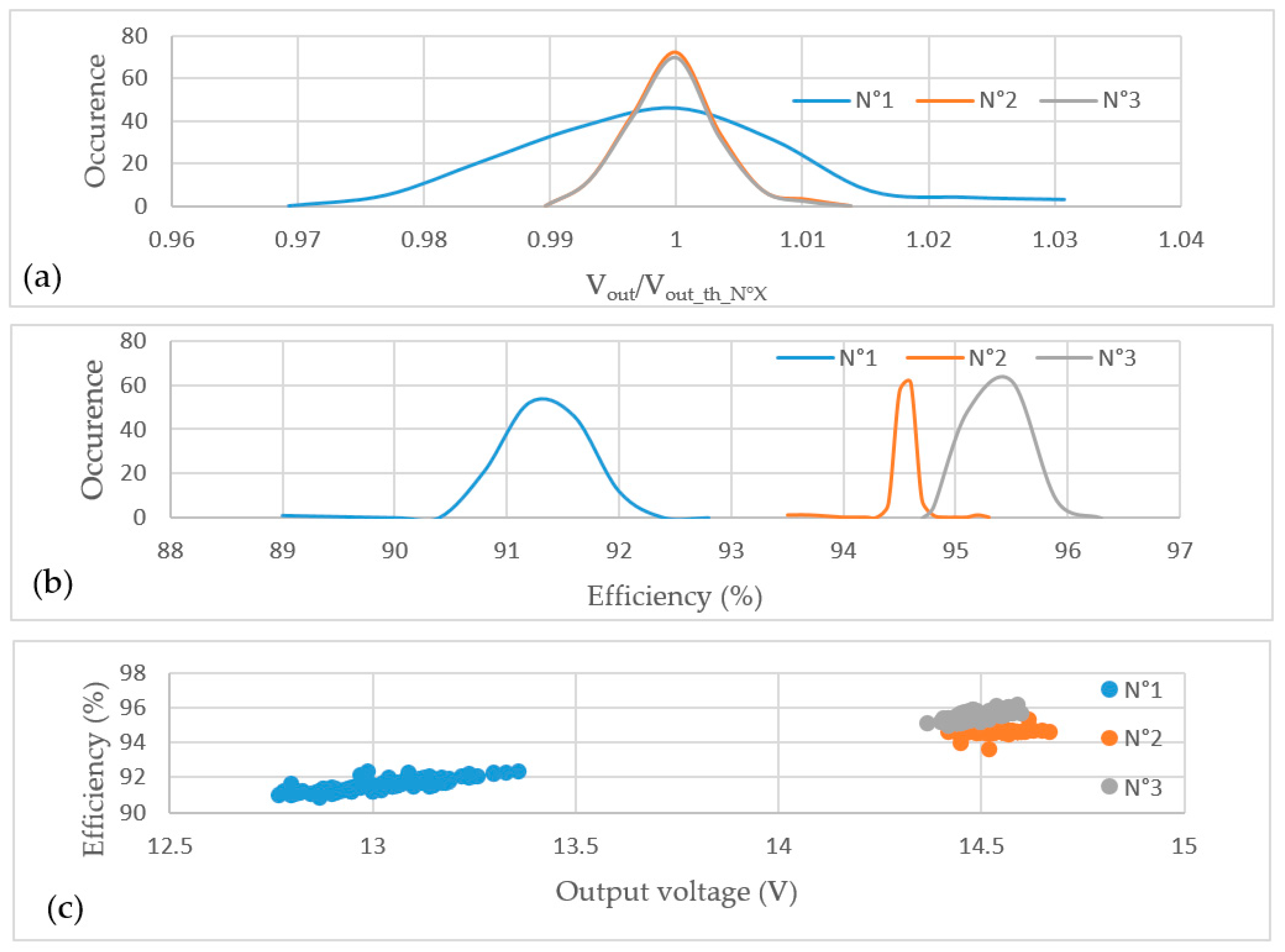
Three families of 3 CSCs have been selected from the 3 extremes quintiles (explained in Section 3.2) in the Gaussian distribution and have been further characterized. Each CSC is named CSC_y,z, where the y variable represents the family letter (A, B and C) and the z variable represents the number of the CSC in that family (1, 2 and 3). With 9 CSCs, arrangements above 360k are still possible. This is not possible and the experiment must be narrowed.

Table 5. Design of experiment with 3 × 3 CSC families.

Configuration	Arrangement of y,z (CSCy,z) on Test Bench			Configuration	Arrangement of CSCs on Test Bench
IPOS	B1	B2	B3	ISOP	B1	B2	B3
	A1	A2	A3		A1	A2	A3
	C1	C2	C3		C1	C2	C3
	C1	C2	A1		C1	C2	A1
	C1	A1	A2		C1	A1	A2
	C1	B1	A1		C1	B1	A1
	B1	C1	A1		B1	C1	A1
ISOS	B1	B2	B3	Electrical Test	Input Voltage	Output Voltage	Current
	A1	A2	A3
	C1	C2	C3	N° 1	15 V	13 V	1.5 A
	C1	C2	A1	N° 2	15 V	13.9 V	2.2 A
	C1	A1	A2
	C1	B1	A1
	B1	C1	A1

below describes the design of experiment that has been defined. For each test, 3 sub tests are carried out using 3 sets of CSCs in order to confirm observations. Basically, each CSC family is implemented to highlight the impact of paired CSCs over the distribution range. Only open loop control is investigated in this paper. Then, family mixes are tested. At first, one extreme quintile CSC is introduced in the association. Then one CSC of each family is tested. Finally, respective position of CSCs are changed in order to investigate if the CSC position has an impact. Table 5 does not includes all measurements obtained in order to save some space in the article but also to concentrate data and ease comparisons.

4.2. Bench and Mother Board for Plug and Play ISOP/IPOS/ISOS Configuration Testing

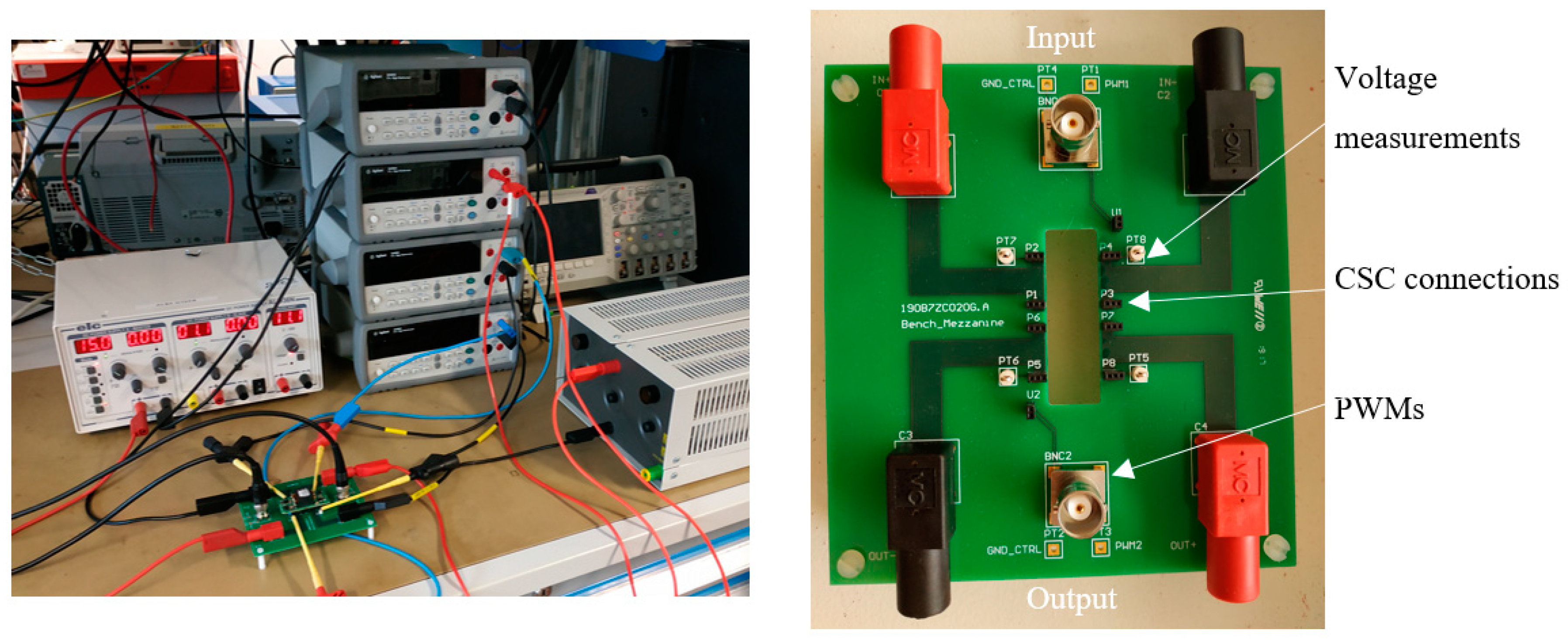
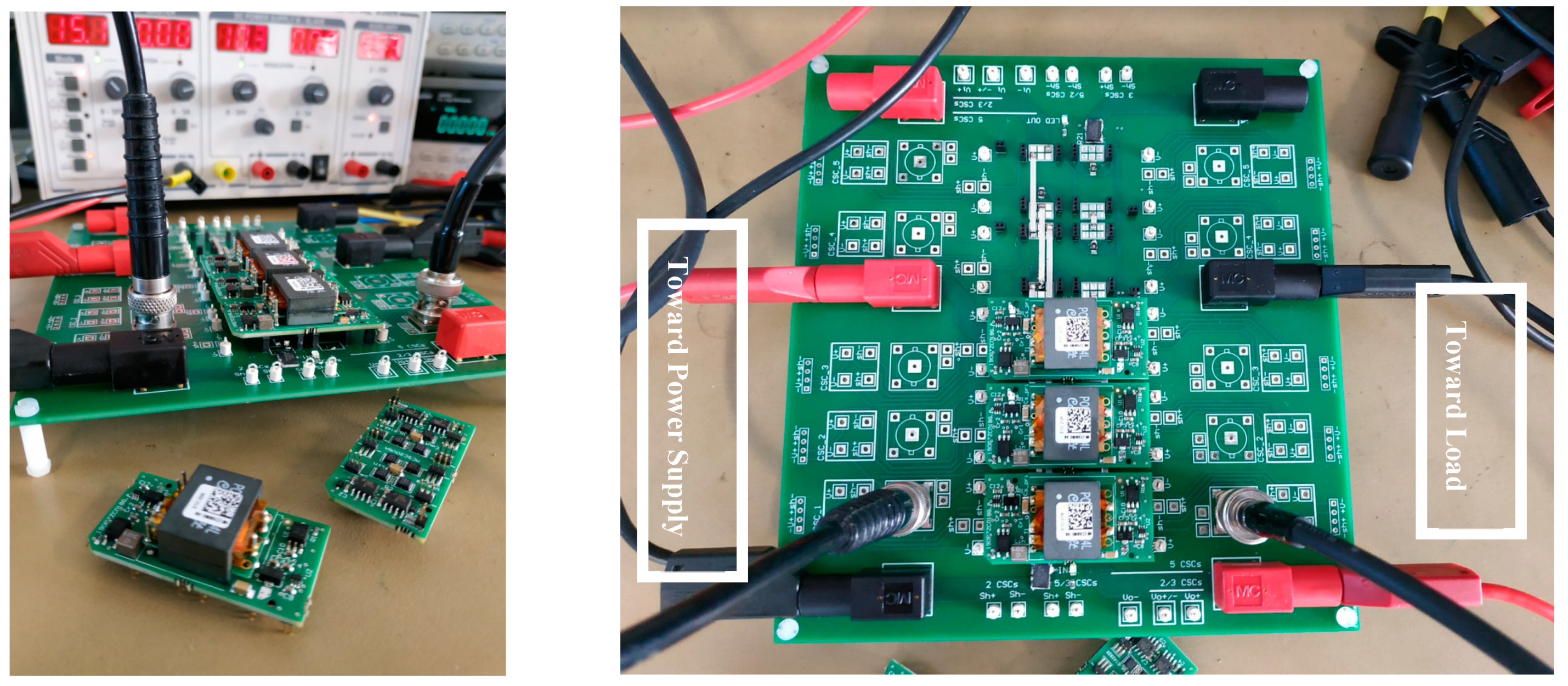
In order to associate and interconnect from the electric point of view the cells presented above to see the impact of the disparity of the components, a test bench has been designed. The test bench used in this test was designed for the balancing test campaign for from 2 up to 5 cells. A mother board was designed to enable any configuration and to ease arrangements. It is presented in Figure 8. This one can implement different configurations (ISOP, IPOS, ISOS) by soldering components not presented in this article. The characteristics are as follows:

• From 2 up to 5 CSCs can be implemented and fully instrumented;
• Any configuration (IPOS, ISOP, ISOS);
• Each cell is instrumented with the same input and output voltage and current measurements device (shunt and kelvin measurements);
• Always the same measurement device are used for the whole experiment and it is always used to measure the same parameters;
• Possibility to apply the same driver signals to the arrangement or possibility to differentiate all of them.

Extreme care was applied to minimize the impact of the mother board. Especially the electrical interconnection among the CSC are carried out with large current rating jumpers, offering very low equivalent resistance (less than 1 mΩ per jumper). Since CSCs are associated on their DC sides, the parasitic inductance of these jumpers has not been considered and further characterized. Indeed, only open loop and steady state operations are considered in this work, where current flowing through jumpers is almost purely DC. As a consequence it is assumed that the inductive contribution of interconnects among CSCs can be neglected. Also, the CSCs are not soldered on the mother board in order to enable and ease the implementation of many arrangement with the same families. For that a specific socket pattern was developed in order to receive the CSC. The impact of such a electrical contact has been carefully checked. The equivalent series resistance of the socket was measured several time over the experiments and remained close to 2 mΩ. The relatively stable value of the resistance, applied in series with all CSC implemented on the board, offers a limited impact. Without being totally negligible, it was not possible to improve further our test bench without a significant complexity in terms of implementation.

All voltage and current (kelvin point on shunt) measurements are carried out with the same 5 digits multi-meters in order to make relative comparison possible. For example, multi-meter 1 always measures CSC input voltage, and so on and so forth. Only up to 3 or 5 CSCs are tested on this bench in order to keep identical the measurements devices and to avoid difficult calibration among measurements devices. This approach, combined with care and methodology, ensures reproducible as well as comparable measurement.

The tests followed the experimental design defined in Table 5. This test was realized in two operating points that are closed to Test 1 and Test 3. Only the main result are shown in this section.

4.3. Experimental Results

Many different studies and analysis can be carried out with the CSC batch that has been produced and characterized. In the following section we are reporting on the very first observations that have been done in a tentative way to illustrate in the most accessible approach.

4.3.1. Electrical Balance Operating Point

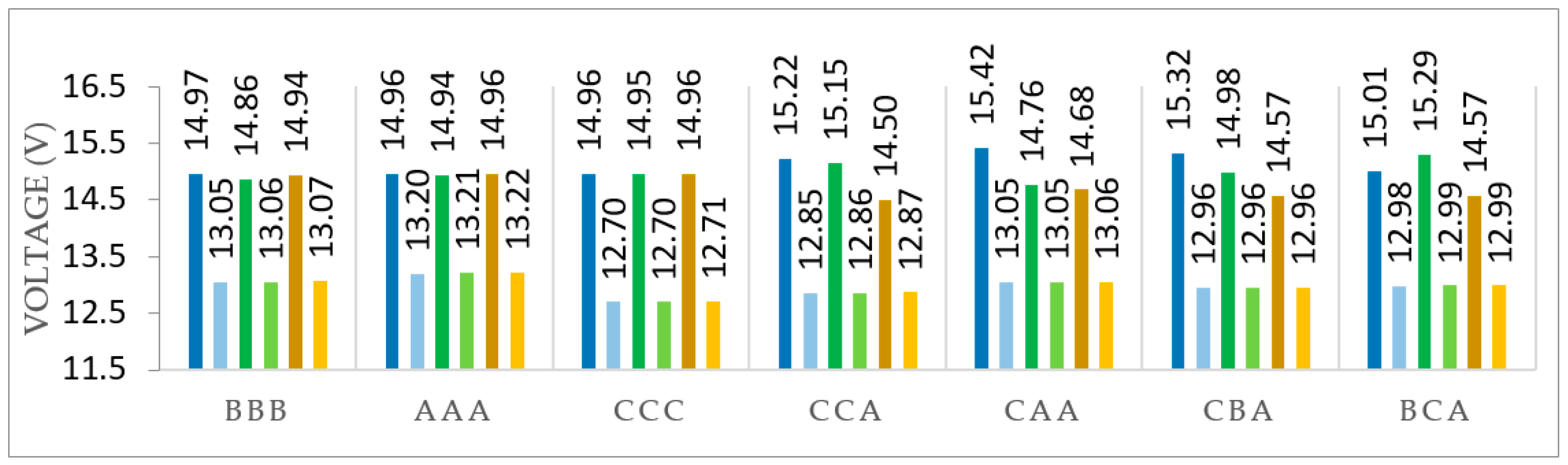
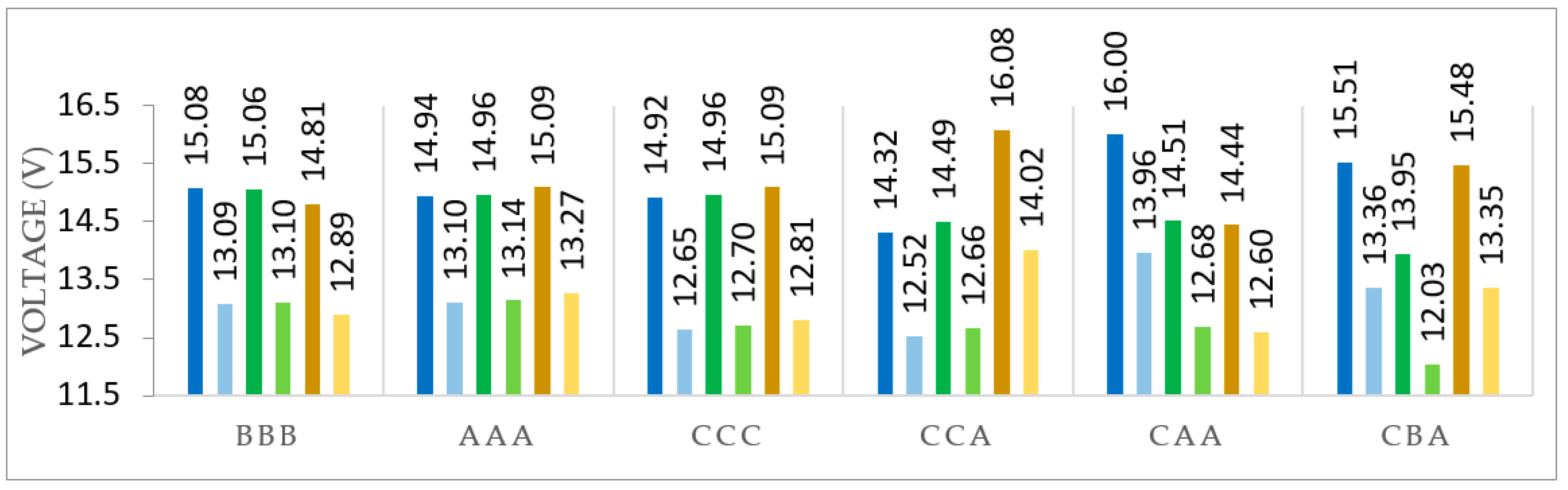
In Figure 9 below, a first set of arrangement testing in IPOS configuration is provided. Several arrangements of 3 CSCs from various families are tested. The letter at the bottom of each test describes the arrangement with respect to the family name. Since it does not add a significant complement, the number of the CSC within the family is not depicted here to optimize the amount of data made available. Each CSC in the arrangement has a color code: blue colors corresponds to the first CSC in the network, green, the second one and yellow the third one. Dark colors counts for input voltage whereas light colors stands for output voltage level. 7 arrangements are displayed. For example, in arrangement number 4, CSC number 2 is coming from family C and has an input voltage of 14.94 V and an output voltage of 12.71V.

In the IPOS configuration, input voltage is fixed by the supply and is equal for all CSCs implemented. In this configuration, for all arrangement, there is a quite good correspondence between the behavior of the CSC when it is implemented alone and when it is implemented into a network. No matter the arrangement and the family, there is almost no issue observed in this configuration. Only a little increase in tendencies can be observed.

When the ISOP configuration is implemented, the input voltage is no more fixed. It is now the output voltage that is made common to all CSCs due to the selected configuration. In an open loop, R load primary to secondary phase shift are fixed, together with the total input voltage, equal to 45 V. In that case, the output voltage is left free to stabilize at any voltage level, as well as the CSC input voltages that only constraint is that the sum must remain equal to 45 V.

As long as arranged CSCs are coming from the same family, only little variation is observed. When family is mixed, a clear observation can be made. The output voltage becomes dependent on the distribution of the families. Basically it can be simplified saying that the output voltage becomes the averaged voltage function of the number of CSC coming from each family. Considering that a family is defined by an identical output voltage, then the output voltage is defined by the Equation (2). Equation (2) can be applied to all the balance voltages in Figure 10.

$$V_{out}=\frac{i_A\ast V_{ou{t}_{AAA}}+i_B\ast V_{ou{t}_{BBB}}+i_C\ast V_{ou{t}_{CCC}}}{3}$$

(2)

$i_X$: number of X family CSC, $V_{OU{T}_{XXX}}$: Output voltage for XXX arrangement.

Apart from this observation, the ISOP configuration is also quite resilient to CSC characteristic dispersion.

In the ISOS configuration presented in Figure 11, neither the input voltage of each CSC nor their respective output voltage are fixed. Only the total voltage at the input must be equal to the supply. The total output voltage is left free to reach any level. Only R load, phase shift and total input voltage are fixed in this test. In this configuration, the dispersion introduced by the CSCs is significantly magnified. As reported in the literature [19], ISOS configuration is really more sensitive to component tolerance. In the proposed case study, all tendencies are respected but magnified. This means that closed loop control could be implemented at converter levels and that there is no need here to implement dedicated control to each CSC. This comment remains to be validated with tests under closed loop control which has not been implemented at this stage of the study.

Apart from these considerations, comments applicable to the three tests can be made. It has been observed that, in the tested conditions, no matter the configuration, the relative position of a fixed set of CSCs within the arrangement has no observable influence on the global behavior of the global converter.

It appears that quintile classification is good enough to say that devices that are contained within the same quintile will behave properly no matter the configuration implemented or tested.

In order to complete the study, an electrical test of point N° 2 (Table 5) was carried out. This is done at higher power but with a lower input-output voltage delta. Figure 12 shows the SIPO association on point N° 2. The same conclusions can be drawn as above.

4.3.2. Losses Aspect of Power Converter Array (PCA)

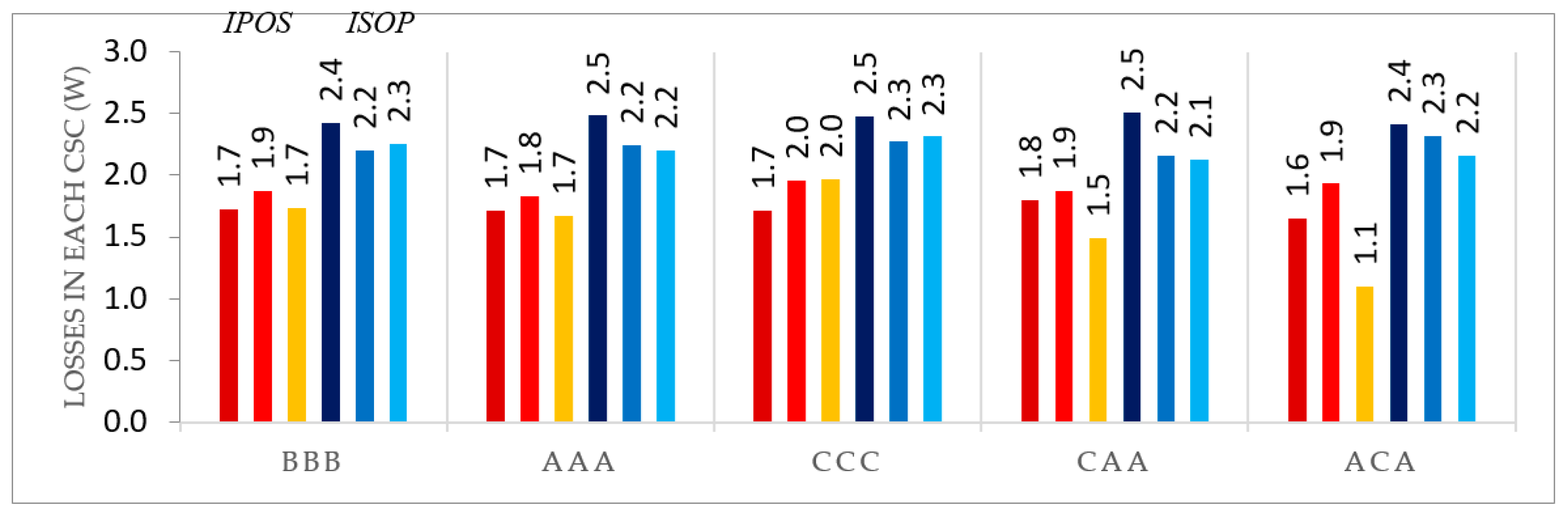
Figure 13 shows, with several graphs, the distribution of losses in each cell according to the arrangement for the IPOS and ISOP configurations. Red colors correspond to IPOS configuration whereas blue colors correspond to the ISOP configuration. For example, the first set of three bars in red colors in Figure 13 represent the losses in each CSC for a configuration of 3 associated CSCs in IPOS.

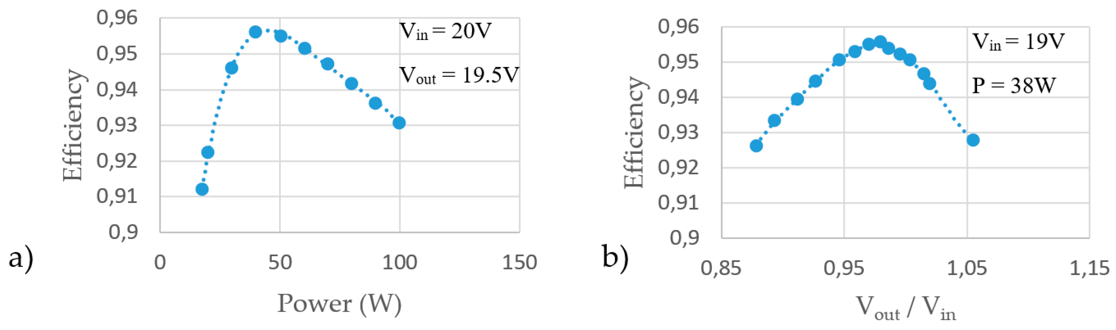
Overall, it is possible to see that losses are balanced as soon as the cells are from the same family while these losses are naturally more unbalanced in the case of a family mix. It is necessary to specify again that only one command is sent for the 3 CSCs and that the regulation is not done at the cell level. This imbalance is induced by output voltage variations which has a great impact on effiency and, therefore, losses as shown in Figure 3.

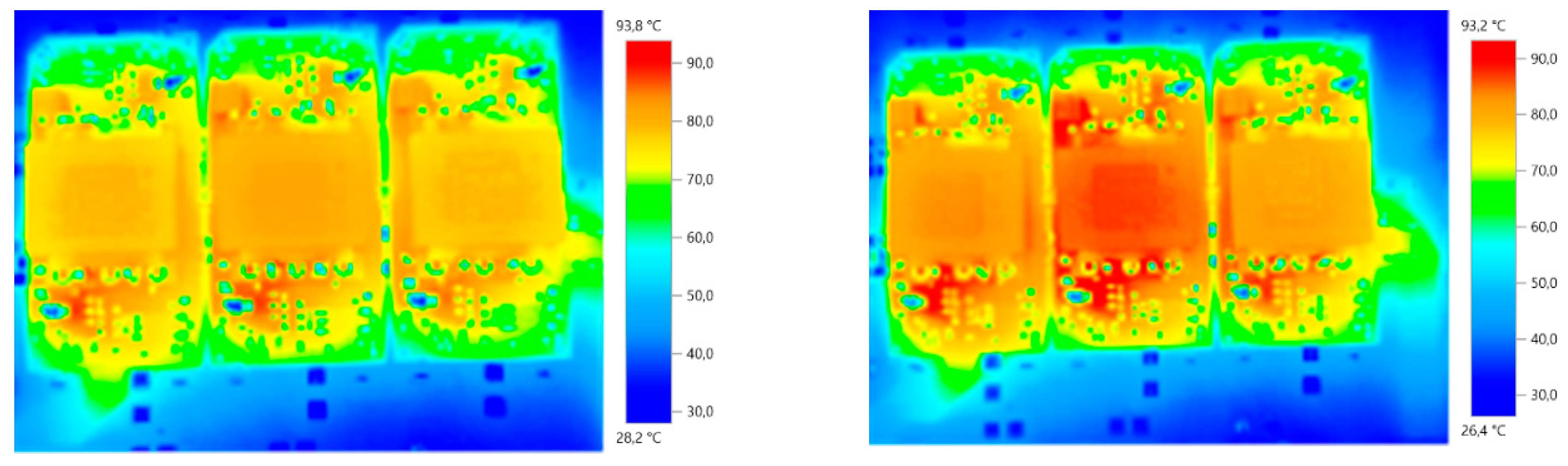
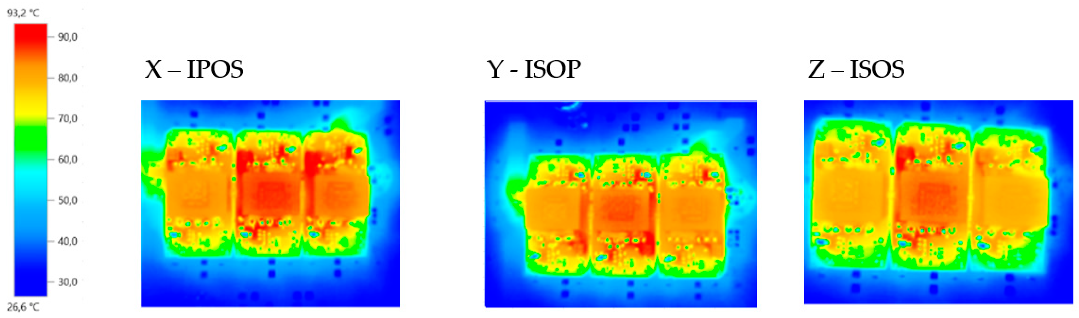
This deviation necessarily leads to a temperature rise that can be critical, as shown in the following thermal photos in Figure 14.

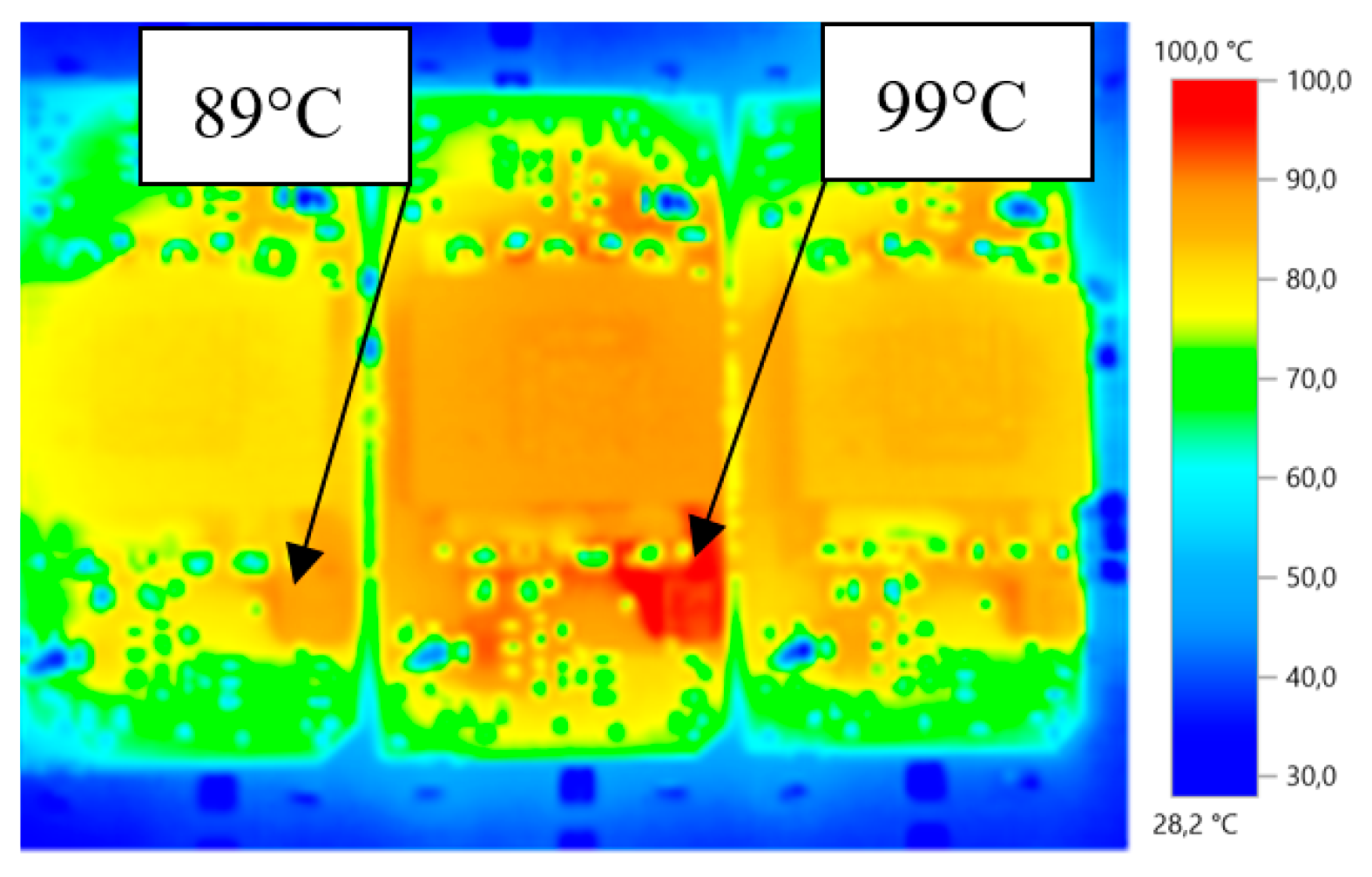
On the thermal image above, a difference in the overall temperature of the cells according to their family is clearly visible. In Figure 14, it is possible to measure up to 5 °C deviation over the same configuration if the cells are in extreme quintile (3 “C” CSCs or 3 “A” CSCs). For arrangements with mixed families, a more significant deviation can occur and bring a cell to a critical temperature as shown in Figure 15. Some other arrangements and configurations which are not part of electrical Tests 1 and 2 presented in Table 5 have showed that it can reach 10 °C deviation on two CSCs on the same PCA. This phenomenon is illustrated in Figure 15. These observations should obviously be taken into consideration while designing the thermal cooling system.

4.3.3. Full Comparison of a PCA of CAA Family CSCs and a 5 CSCs ISOS Configuration

This part is investigating at first if three identical CSCs coming from a family mix may operate in a different manner depending on the configuration. The 3 CSCs are, from left to right, coming from family CAA. This choice is purely arbitrary, the goal being to see if there is a clear impact of the configuration on CSC behavior. The study provides, in

Table 6. Measures at CSC level of various PCA configurations with the same CAA arrangement.

	CSC1			CSC2			CSC3
Test	Vin	Vout	η	Vin	Vout	η	Vin	Vout	η
X-IPOS	15.11 V	13.78 V	94.8%	15.10 V	13.99 V	94.6%	15.13 V	13.98 V	95.6%
Y-ISOP	15.24 V	13.96 V	92.7%	15.04 V	13.96 V	93.5%	14.93 V	13.90 V	93.4%
Z-ISOS	15.57 V	14.29 V	95.1%	14.87 V	13.63 V	94.1%	14.86 V	13.62 V	95.5%

, for each configuration (IPOS/ISOP/ISOS) the operating point of each cell and Figure 16, a thermal image of the PCA for each configuration.

These observations bring to light that ISOP configuration seems to be the worst case in terms of losses and efficiency. This result hides the important fact that CSCs operating points are significantly different due to absence of fixed voltage reference at the CSC input terminals. In such a way, CSCs are moving away from the optimal operating point, lowering their efficiency. This observation, which is valid for this case, may not always apply. Nonetheless, it shows that there are operating points that are leading to significant increase of losses.

Second, the ”weakest” CSC, understanding the cell with the lowest efficiency, remains the same no matter the configuration. This phenomenon is magnified due to the geographically positioned CSC in the middle always being warmer.

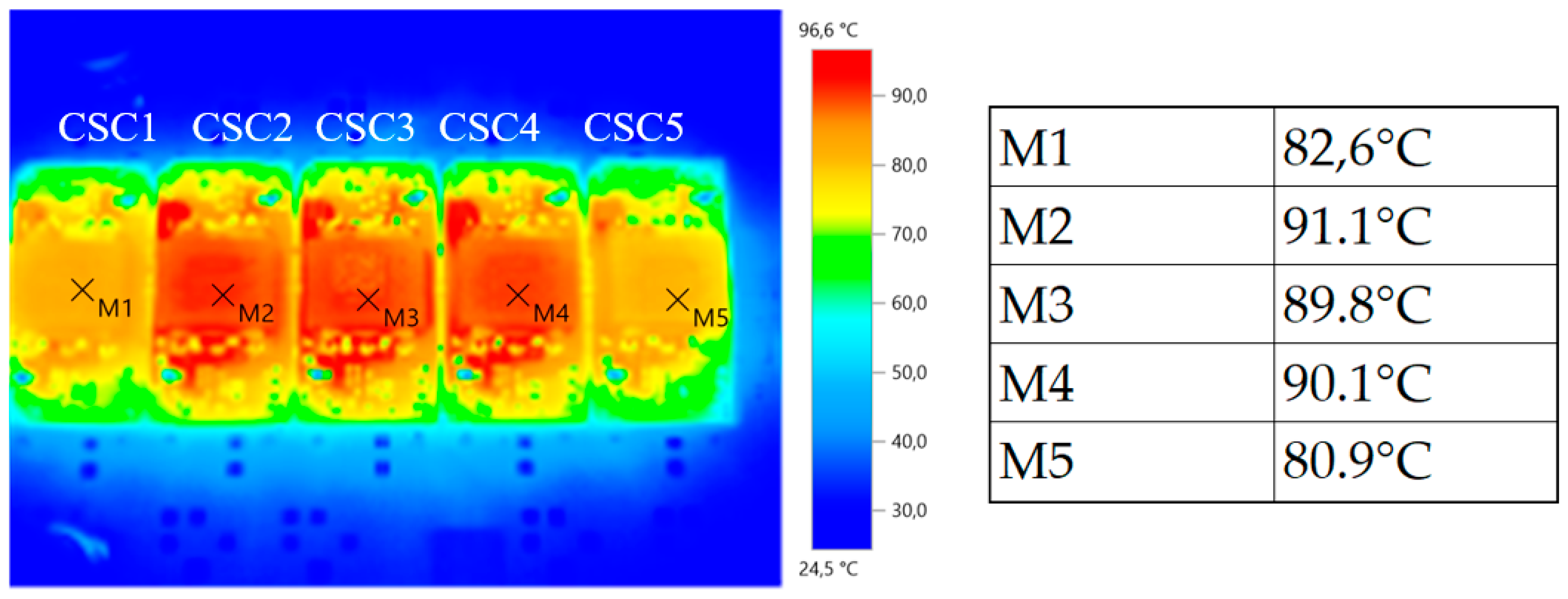
A second study shows a case study with 5 CSCs in ISOS configuration only. Until now, there were no results for 5 CSCs.

Table 7. PCA of 5 BBCBA CSCs configured in ISOS.

Test	CSC1: B		CSC2: B		CSC3: C		CSC4: B		CSC5: A
η (%)	Vin	Vout	Vin	Vout	Vin	Vout	Vin	Vout	Vin	Vout
94.8	14.95 V	13.49 V	14.94 V	13.48 V	15.11 V	13.67 V	15.22 V	13.75 V	14.69 V	13.26 V

shows the voltage and current distributions by cell for the following arbitrary family arrangement from left to right: BBCBA. This arrangement is representative of reality because, as shown in Figure 5, there are few CSCs in family C and A which are coming from the extreme quintiles.

Several things can be noticed in Table 7 and Figure 17. The voltages of the first two CSCs (CSC1 and CSC2) of the B family are stable. CSC4 of family B does not have the same set of tensions This phenomenon is still under investigation. CSCs C and A have higher and lower voltages, respectively, than the tests done in the previous parts. On the thermal part, we notice that the external CSCs benefit from a lower temperature due to their peripheral placement. CSC2, CSC3 and CSC4 have the same temperature as shown in Figure 1 while they have a different electrical operating point as shown in Table 7. It can therefore be concluded that the disparity of the components during the ISOS configuration is smoothed at the thermal level but remains strong at the electrical level. Despite the differences in the electrical operating points of the CSCs, thermal images allow us to conclude that the placement of the CSC has a significant influence on its thermal equilibrium point. Nonetheless, Figure 17 that the CSCs dispersion remains visible since the CSC at the middle of the array is colder than its direct neighbors. A relative impact of CSCs dispersion versus their physical position in the array could be considered in a future work.

4.4. Discussion of Main Results

Regarding the CSC batch characterization, it is important to highlight a few observations:

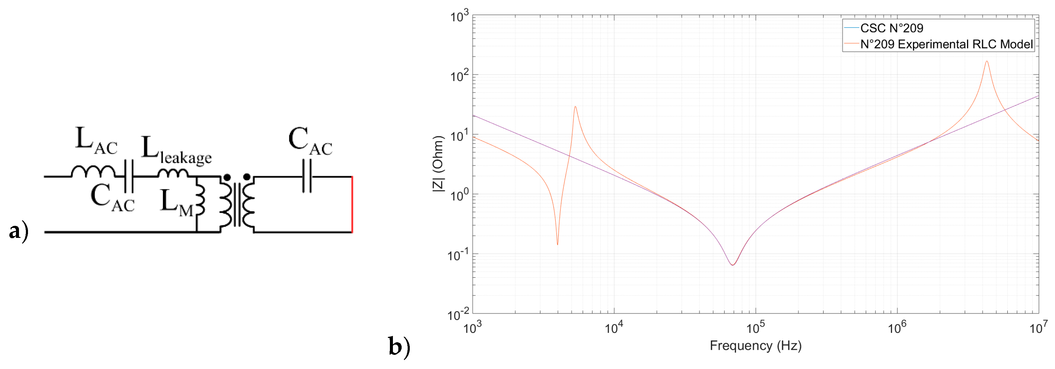
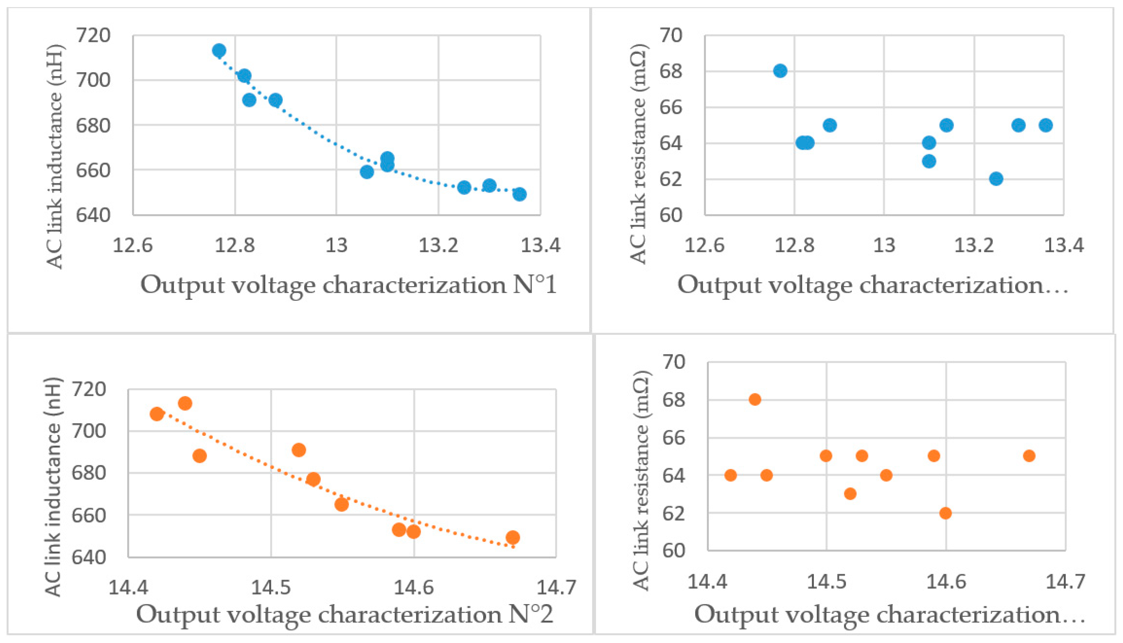
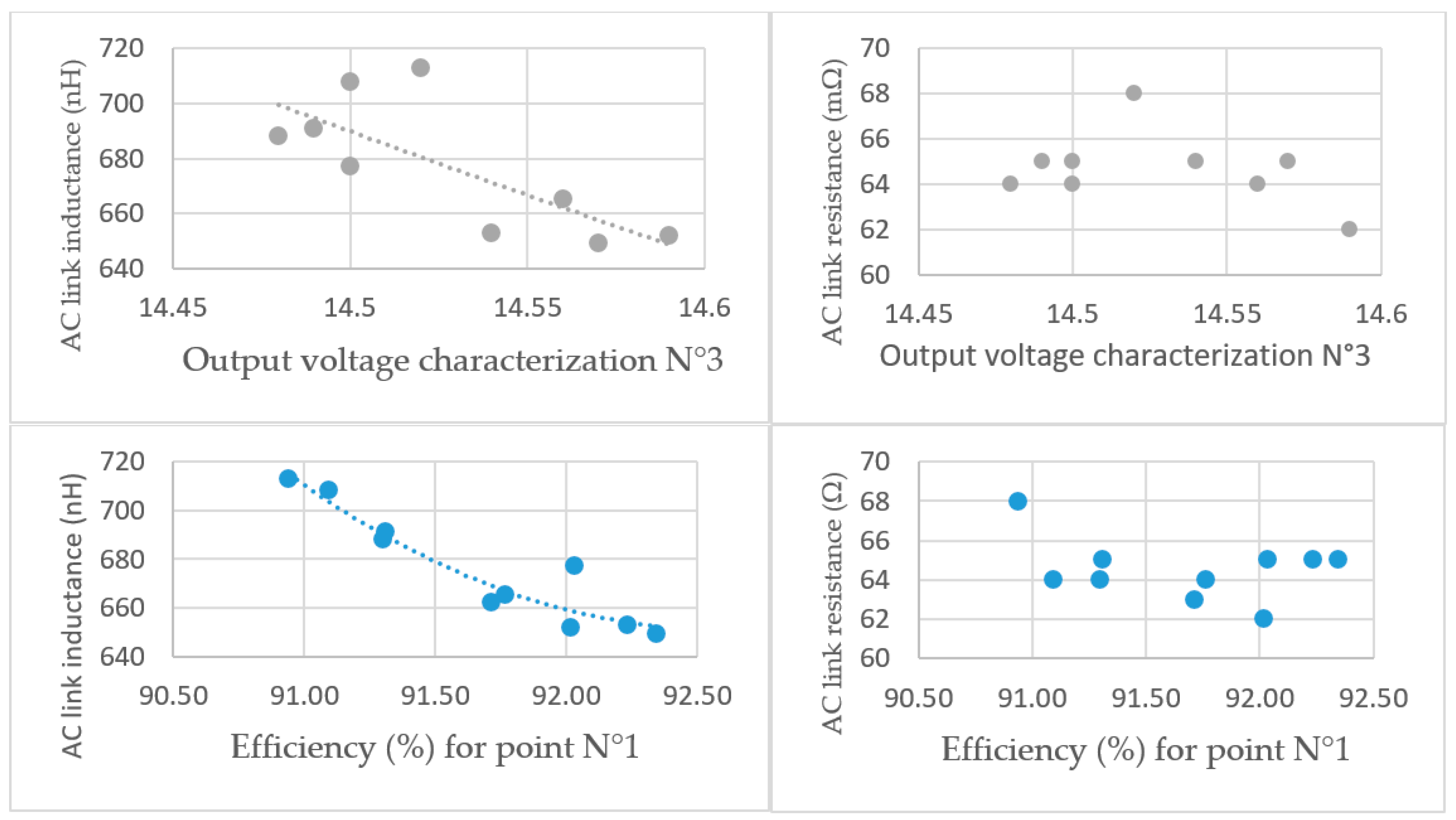
First of all, manufactured after a significant industrialization process, the CSCs remain slightly unpaired. This is mostly due to components that are provided by suppliers with tolerances. In our very specific example, CSCs are manufactured on PCBs and are all made out of off the shelf components with regular tolerances between 1% to 20%. Of course, the converter remains sensitive to the components’ main parameters. It appears, as a first result that the AC link inductor in DAB based topology is the most significant and critical component. Its sensitivity can be mathematically proven based on Equation (1). The tolerance on its value induces a tolerance on the whole DAB converter in terms of operating point, including CSC efficiency level. From that, it becomes important to frame the component tolerance such that it remains within good limits according to its application. In the case of the DAB converter, the tolerance on the total AC inductor introduces a large enough tolerance on the converter performances that it needs further investigations. Especially, in the presented case, CSCs being networked, it becomes critical to evaluate the impact of the converter operating point tolerance other an array of CSCs.

Regarding CSCs networks, some additional comments can be drawn:

Several CSC family arrangements have been implemented and characterized in three different configurations. ISOP, IPOS and ISOS were tested specifically because they are the three configuration for which a voltage unbalance among CSCs is possible either at the input or at the output terminals. These tests have been carried out at first in order to investigate how associations of CSCs with different voltage operating points would behave from that point of view. As a reminder, only an open loop was tested in this paper because closed loop control, although being impacted by cell imbalances, is not the purpose of this study.

Analyzing the results above, several comments can be made. First of all, the CSC operating point dispersion clearly affect the input and/or output voltage balance among cells. Paired CSCs have a more favorable behavior no matter the configuration. When arrangement involves CSCs from various families, their characteristic dispersion is mainly confirmed or even enhanced which may become an issue. Voltage imbalances induce efficiency unbalances. The total losses coming from the converter association are always higher than the sum of the losses gathered at cell levels for their expected operating point. This may have a significant impact on thermal management at the cell level.

In particular, it has been observed that in ISOP and ISOS configurations, the individual CSC behavior mismatches are enhanced by the network association. In fact, this is happening whenever the input voltage of the CSC is not fixed by the implementation. On the other side, IPOS configuration is very resilient to CSC characteristic tolerances.

From this analysis several options can be foreseen:

Provision must be taken while designing the thermal cooling. Considering the technology considered in this work, the PCB based CSCs are cooled down with air flow. With natural air cooling, CSCs’ current rating may have to be reduced to account for operating point variability and consecutive losses mismatches. With forced air cooling, increasing the air speed may compensate the losses mismatch among CSCs.

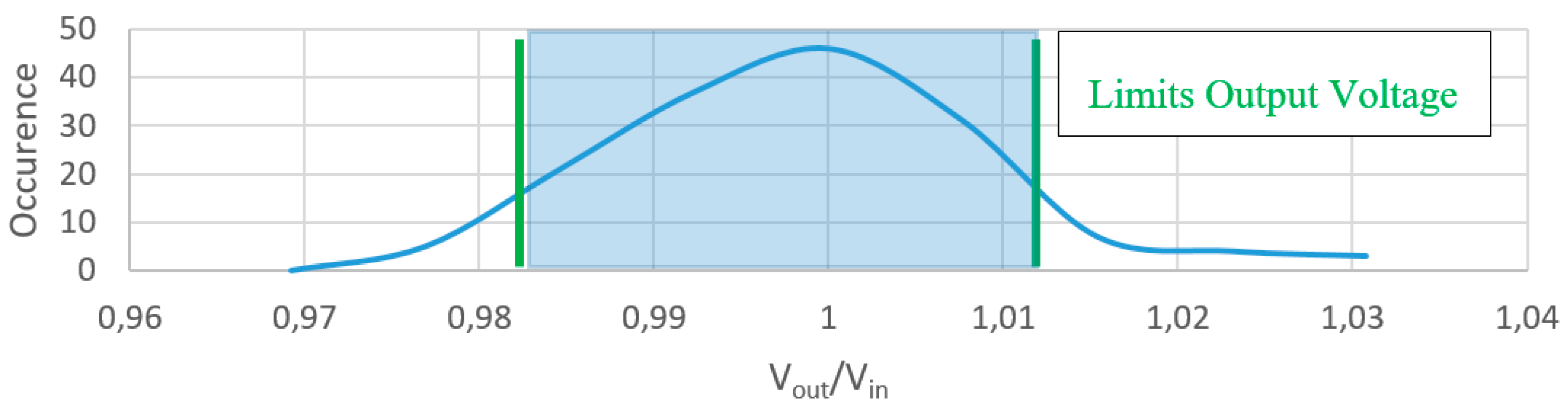
Since a functional testing is carried out after batch production, this test could include a short characterization of the meaning full operating point. The paper has clearly highlighted the relation between the component tolerance and their impact on converter operation and more specifically the output voltage with respect to all other parameter constant.

The functional test could be used to sort CSCs in quintile or even decile. In such a way, PCAs could be produced from paired CSCs, levering up voltage and current balancing among cells no matter the configuration.

The functional test could be used to remove CSCs that are too much out of a reasonable tolerance. For that, a good tradeoff between the tolerance window and the yield has to be found in order to remain reasonable from a cost point of view. Figure 18 below presents an illustration of that process.

If sorting CSCs ends up to be too much unproductive or costly, another option is to work on the tolerance of the most critical components, probably the HF transformer and possibly the AC link additional inductor. Working on these two devices, sorting or selecting them could be a first option less costly than the whole CSC. Of course, this would require developing a test routine to sort components according to the leakage inductance for the HF transformer and the value of the inductor as far as the L_AC inductor is concerned. Also, a specific work with the supplier could be carried at design and technological levels in order to narrow the tolerance on the components.

5. Conclusions

The paper has presented the first analysis carried out on the impact of component tolerance on arrays of power conversion cells. Based on over 130 samples, a characterization process has been carried at CSC level in order to identify the most critical components from an experimental point of view. Based on a classification, the impact of component tolerance on CSC operating points when implemented in various configurations ISOP, IPOS and ISOS has been investigated. It has been shown that when CSC input voltage is not imposed on CSCs, their behavior mismatches are enhanced. From this, several guidance notes are provided in a tentative to minimize the impact of component tolerance on the implementation of a PCA. The analysis is valid for the topology used in this work and the technology and components used also and they are not generalized at this stage of the study. It is mainly the methodology that is reported. Some interesting results and comments are provided to guide future PCA implementation.

References

1. Engel, S.P.; Stieneker, M.; Soltau, N.; Rabiee, S.; Stagge, H.; De Doncker, R.W. Comparison of the Modular Multilevel DC Converter and the Dual-Active Bridge Converter for Power Conversion in HVDC and MVDC Grids. IEEE Trans. Power Electron. 2015, 30, 124–137. [Google Scholar] [CrossRef]
2. Kasper, M.; Bortis, D.; Kolar, J.W. Scaling and balancing of multi-cell converters. In Proceedings of the 2014 International Power Electronics Conference, Hiroshima, Japan, 18–21 May 2014; pp. 2079–2086. [Google Scholar]
3. Younsi, M.O.; Bendali, M.; Azib, T.; Larouci, C.; Marchand, C.; Coquery, G. Current-sharing control technique of interleaved buck converter for automotive application. In Proceedings of the 7th IET International Conference on Power Electronics, Machines and Drives (PEMD 2014), Manchester, UK, 8–10 April 2014; pp. 1–6. [Google Scholar]
4. Chen, R.; Zeng, H.; Gunasekaran, D.; Liu, Y.; Peng, F.Z. Development of 2-kW interleaved DC-capacitor-less single-phase inverter system. In Proceedings of the 2016 IEEE Applied Power Electronics Conference and Exposition (APEC), Long Beach, CA, USA; 2016; pp. 1045–1050. [Google Scholar]
5. Anzari, M.; Meenakshi, J.; Sreedevi, V.T. Simulation of a transistor clamped H-bridge multilevel inverter and its comparison with a conventional H-bridge multilevel inverter. In Proceedings of the 2014 International Conference on Circuits, Power and Computing Technologies [ICCPCT-2014], Nagercoil, India, 20–21 March 2014; pp. 958–963. [Google Scholar]
6. Dargahi, V.; Sadigh, A.K.; Abarzadeh, M.; Pahlavani, M.R.A.; Shoulaie, A. Flying Capacitors Reduction in an Improved Double Flying Capacitor Multicell Converter Controlled by a Modified Modulation Method. IEEE Trans. Power Electron. 2012, 27, 3875–3887. [Google Scholar] [CrossRef]
7. Ericsen, T.; Tucker, A. Power Electronics Building Blocks and potential power modulator applications. In Proceedings of the Conference Record of the Twenty-Third International Power Modulator Symposium, Rancho Mirage, CA, USA, 25 June 1998; pp. 12–15. [Google Scholar]
8. Ericsen, T.; Khersonsky, Y.; Steimer, P.K. PEBB Concept Applications in High Power Electronics Converters. In Proceedings of the 2005 IEEE 36th Power Electronics Specialists Conference, Recife, Brazil, 16 June 2005; pp. 2284–2289. [Google Scholar]
9. Andreta, A.G.; Lamorelle, T.; Lembeye, Y.; Kerachev, L.; Sarrafin, F.; Fernando, L.; Villa, L.; CrebierMetrics, J.C. A High Efficiency and Power Density, High Step-Up, Non-isolated DC-DC Converter Based on Multicell Approach. In Proceedings of the CIPS 2018 10th International Conference on Integrated Power Electronics Systems, Stuttgart, Germany, 20–22 March 2018; pp. 1–5. [Google Scholar]
10. Lamorelle, T.; Nguyen, S.; Podvin, J.C.; Rubio, D.; Lembeye, Y.; Crebier, J. Multi-cell DC-DC converters - Input differential mode filtering generic design rules and implementation. In Proceedings of the PCIM Europe 2019-International Exhibition and Conference for Power Electronics, Intelligent Motion, Renewable Energy and Energy Management, Nuremberg, Germany, 7–9 May 2019; pp. 1–8. [Google Scholar]
11. Sarrafin-Ardebili, F.; Crebier, J.-C.; Allard, B. Quad Driver for GaN transistors based Dual Active Bridge with capacitive coupling. In Proceedings of the 2018 IEEE International Conference on Industrial Technology (ICIT), Lyon, France, 20–22 February 2018. [Google Scholar]
12. Liang, Z.; Lee, F.C.; Lu, G.Q.; Borojevic, D. Embedded power-a multilayer integration technology for packaging of IPEMs and PEBBs. In Proceedings of the IWIPP 2000. International Workshop on Integrated Power Packaging (Cat. No.00EX426), Waltham, MA, USA, 14–15 July 2000; pp. 41–45. [Google Scholar]
13. Lamorelle, T.; Andreta, A.; Lembeye, Y.; Crébier, J.-C.; Podvin, J. Design level power electronics building block: Industrial framework for DC-DC conversion. In Proceedings of the 2018 IEEE International Conference on Industrial Technology (ICIT), Lyon, France, 20–22 February 2018; pp. 670–675. [Google Scholar]
14. Kerachev, L.; Lembeye, Y.; Andreta, A.; Crebier, J. Generic Approach for Design, Configuration and Control of Modular Converters. In Proceedings of the PCIM Europe 2017-International Exhibition and Conference for Power Electronics, Intelligent Motion, Renewable Energy and Energy Management, Nuremberg, Germany, 16–18 May 2017; pp. 1–8. [Google Scholar]
15. Chauhan, D.; Liu, P.; Patil, M.; Rao, S. Statistical analysis of mismatch error in series and parallel connection of photovoltaic. In Proceedings of the 2011 Annual IEEE India Conference, Hyderabad, India, 16–18 December 2011; pp. 1–5. [Google Scholar]
16. Almeida, A.d.O.; Ghetti, F.T.; Ribeiro, A.S.B.; de Almeida, P.M.; Barbosa, P.G. Circulating currents suppression strategies for modular multilevel converter. In Proceedings of the 2017 Brazilian Power Electronics Conference (COBEP), Juiz de Fora, Brazil, 19–22 November 2017; pp. 1–5. [Google Scholar]
17. Andreta, A.; Derbey, A.; Lembeye, Y.; Villa, F.L.L.; Crebier, J. Characterization Platform for Modular Power Converters. In Proceedings of the PCIM Europe 2018-International Exhibition and Conference for Power Electronics, Intelligent Motion, Renewable Energy and Energy Management, Nuremberg, Germany, 5–7 June 2018; pp. 1–6. [Google Scholar]
18. Ayyanar, R.; Giri, R.; Mohan, N. Active input-voltage and load-current sharing in input-series and output-parallel connected modular DC-DC converters using dynamic input-voltage reference scheme. IEEE Trans. Power Electron. 2004, 19, 1462–1473. [Google Scholar] [CrossRef]
19. Bottion, A.J.B.; Barbi, I. Series-series association of two Dual Active Bridge (DAB) converters. In Proceedings of the 2015 IEEE International Conference on Industrial Technology (ICIT), Seville, Spain, 17–19 March 2015; pp. 1161–1166. [Google Scholar]
Figure 1. (a) Input series/output parallel (ISOP), input parallel/output series (IPOS) and input series/output series (ISOS) configuration illustration, (b) topology of a dual active bridge (DAB) converter.
Electronics 08 00917 g001
Figure 2. Picture of a single conversion standard cell (CSC) based on the DAB topology (left), picture of a power converter array (PCA), made with 16 CSCs, arranged in 4 columns, 2 lines and 2 boards (right).
Electronics 08 00917 g002
Figure 3. Two typical characteristics of DAB converter efficiency. (a) efficiency versus output current, (b) efficiency versus input, output voltage difference. Other operating point parameters available in the figure.
Electronics 08 00917 g003
Figure 4. Picture of the characterization board, together with the instrumentation required to carry out CSC testing.
Electronics 08 00917 g004
Figure 5. Statistic distributions of CSCs. (a) distribution of output voltage (b) distribution of efficiency rating (c) distribution of efficiency versus output voltage level for the three test campaigns.
Electronics 08 00917 g005
Figure 6. (a) One AC link branch impedance characterization for the 3 × 3 CSCs on impedance analyzer (Keysight E4990A) (b) One on the impedance plot versus frequency (only one curve is provided since they are superposed due to only small differences.
Electronics 08 00917 g006
Figure 7. Correlation curves between AC link equivalent inductor value and CSC output voltage and efficiency and equivalent resistor versus output voltage.
Electronics 08 00917 g007aElectronics 08 00917 g007b
Figure 8. CSCs in front of test bench. Experimental setup test bench.
Electronics 08 00917 g008
Figure 9. Voltage balance in CSCs depending on association at operating point N° 1 in IPOS config.
Electronics 08 00917 g009
Figure 10. Voltage balance in CSCs depending on association at operating point N° 1 in ISOP config.
Electronics 08 00917 g010
Figure 11. Voltage balance in CSCs depending on association at operating point N° 1 in ISOS config.
Electronics 08 00917 g011
Figure 12. Voltage balance in CSCs depending on association at operating point N° 2 in ISOP config.
Electronics 08 00917 g012
Figure 13. Losses in CSCs depending on association at operating point N° 2 in IPOS and ISOP.
Electronics 08 00917 g013
Figure 14. ISOP configuration of CSCA,1 CSCA,2 CSCA,3 (left) and CSCC,1 CSCC,2 CSCC,3 (right) in same electrical configuration for electrical Test 2.
Electronics 08 00917 g014
Figure 15. Thermal image of ACA arrangement for the following operating point of Vin = 45 V; Vout = 13.7 V; Pout = 90 W.
Electronics 08 00917 g015
Figure 16. Thermal images of various PCA configurations with the same CAA arrangement.
Electronics 08 00917 g016
Figure 17. Thermal image of ISOS BBCBA arrangement with the following parameters Vin = 75 V; Vout = 67.5 V; Pout = 150 W.
Electronics 08 00917 g017
Figure 18. Illustration of window tolerance out of which CSC are declared out of the spec and removed from the supply chain.
Electronics 08 00917 g018