Optimal Feature Search for Vigilance Estimation Using Deep Reinforcement Learning
by
 , ,
, ,
Woojoon Seok
1 ,
,
Minsoo Yeo
2,
Jiwoo You
2,3,
Heejun Lee
2,
Taeheum Cho
1,
Bosun Hwang
4 and
Cheolsoo Park
2,* 1
Intelligent Information System and Embedded Software Engineering, Kwangwoon University, Seoul 01897, Korea
2
Department of Computer Engineering, Kwangwoon University, Seoul 01897, Korea
3
Faculty of Science and Engineering, Rijksuniversiteit Groningen, 9727 Groningen, The Netherlands
4
Department of Computer Science and Engineering, Seoul National University, Seoul 08826, Korea
*
Author to whom correspondence should be addressed.
Electronics 2020, 9(1), 142; https://doi.org/10.3390/electronics9010142
Submission received: 29 November 2019
/
Revised: 2 January 2020
/
Accepted: 6 January 2020
/
Published: 11 January 2020
(This article belongs to the Special Issue The Challenges in Brain-Computer Interface (BCI) - toward Practical BCI)
Abstract
:A low level of vigilance is one of the main reasons for traffic and industrial accidents. We conducted experiments to evoke the low level of vigilance and record physiological data through single-channel electroencephalogram (EEG) and electrocardiogram (ECG) measurements. In this study, a deep Q-network (DQN) algorithm was designed, using conventional feature engineering and deep convolutional neural network (CNN) methods, to extract the optimal features. The DQN yielded the optimal features: two CNN features from ECG and two conventional features from EEG. The ECG features were more significant for tracking the transitions within the alertness continuum with the DQN. The classification was performed with a small number of features, and the results were similar to those from using all of the features. This suggests that the DQN could be applied to investigating biomarkers for physiological responses and optimizing the classification system to reduce the input resources.
1. Introduction
One of the main causes of traffic and industrial accidents is a low level of attention from fatigue, which greatly reduces work efficiency and increases the risk of accidents, and thus, a system automatically detecting the low level of alertness is a highly desirable. The research to estimate drowsiness or lack of vigilance mainly investigates physiological signals and video streaming information (eye blinking and yawning) [1,2]. Video images obtained from a camera could detect with high accuracy, drowsiness, and with low accuracy, vigilance. However, at night time or when wearing sunglasses, it would be difficult to capture the faces of users using the camera. For these cases, physiological signals could help to determine the states of the drowsiness or low level of vigilance. The objective of this study was establishing automatic assessment of vigilance monitoring system with physiological signals using deep reinforcement learning algorithm. The previous studies of alertness estimation mainly utilized the electroencephalogram (EEG), electrocardiogram (ECG), electrooculogram (EOG), and electromyogram (EMG) signals [3,4,5,6,7,8]. A vigilance monitoring system based on physiological signals could be implemented by utilizing EEG, ECG, and EOG signals.
EEG signals are widely utilized in practical situations, including brain computer interfacing (BCI), epileptic seizure prediction, drowsiness detection, and vigilance state analysis [3,9,10,11]. EEG signal analysis is more challenging than other physiological signals because it contains several artifacts and high levels of noises such as EOG, EMG, and ECG signals [12]. The vigilance state study also utilizes the EEG signals and mainly uses the four EEG frequency components [13]. Four frequency components are extracted to make up the features of an EEG signal in the delta (: 0–4 Hz), theta (: 4–8 Hz), alpha (: 8–13 Hz), and beta (: 13–20 Hz) bands [14]. A high amplitude in the delta band corresponds to deep sleep, and a high amplitude in the theta band corresponds to drowsiness [13]. kerstedt et al. used features from frequency components in the theta and alpha bands to predict sleep and drowsiness states [7]. A decreasing power in the alpha frequency band and increasing power in the theta frequency band may be a meaningful drowsiness indicator [6]. Additionally, combinations of theta, alpha, and beta frequency components, such as , , have been used to extract features for detecting the drowsy and fatigued state. Studies on detecting low level of alertness with the EEG signal mainly used frequency-domain features and rarely considered time-domain features [10]. The area, normalized decay, line length, mean energy, average peak amplitude, average valley amplitude, and normalized peak number are the main time-domain features of an EEG signal. ECG signals are widely utilized to predict arrhythmia, coronary artery disease, and paroxysmal atrial fibrillation [15,16,17]. Chui et al. [18] and Sahayadhas et al. [19] considered ECG signals for estimating the drowsiness condition by extracting heart rate variability (HRV) information, which includes time- and frequency-domain analysis.
Recently, deep learning methods have been applied to healthcare data as replacements for conventional feature extraction methods, and have yielded better performances [20,21]. Deep learning automatically detects specific patterns in physiological signals measured using EEG, ECG, and EMG [22]. In healthcare studies, the convolution neural network (CNN) and autoencoder approach have been widely used to extract features from physiological signals [23,24]. Hwang et al. proposed ultrashort-term segmentation of the ECG signal to estimate stressful conditions [25]. While deep learning approaches have outperformed conventional methods for healthcare data analytics, a critical limitation has been encountered. Although deep learning algorithms automatically extract features in a data-driven manner, they are still a black box that fails to provide physiological meaning. Data analysis should yield interpretable outcomes and explain physiological phenomena corresponding to high-level states, such as cognitive or physical conditions [26]. In the present study, relatively more interpretable conventional algorithms and deep learning methods were used to analyze the states, and were compared to explain the outcomes of deep learning approaches.
Reinforcement learning is an area of machine learning where an agent defined in a specific environment recognizes its current state and acts to maximize a future reward among selectable behaviors. Reinforcement learning is suitable for solving sequential decision-making problems. It has recently outperformed humans in many fields (e.g., Go, Atari game) and has also been used for deep learning optimization [27,28,29]. In the present study, features were extracted with conventional and deep learning methods and fed to a reinforcement learning agent to find the optimal feature set. The aim of this study was to find the best features of EEG and ECG for the assessment of vigilance through reinforcement learning, and thus obtain higher accuracy than conventional supervised learning algorithms.
Related Work
Traditionally, the studies to monitor the vigilance state have utilized several physiological signals, such as EEG, ECG, EOG, and EMG [6,7]. Duta et al. applied the deep learning method to EEG signal for the first time [3]. Looney et al. implemented a wearable monitoring system utilizing a one channel ear EEG signal. For the convenience of users, research about building a vigilance monitoring system using single channel EEG has been increased. In recent vigilance state studies, cameras were used to calculate eye closing time to determine vigilance state. In the experiment, subjects were given vigilance tasks, and if the response time was longer than 500 ms, it was labeled as lack of vigilance [30]. Meanwhile, several methods using HRV parameter and CNN analysis for raw-ECG signals have been applied [25]. Lee et al. [31] extracted the HRV parameters and used classifiers such as a support vector machine (SVM), k-nearest neighbors (KNN), a random forest (RF), and a convolutional neural network (CNN) for the driver vigilance monitoring. Janisch et al. [32,33] utilized a reinforcement learning algorithm to solve the sequential decision-making problem, wherein an agent chooses a feature to see or makes a class prediction at each step. This idea has been widely applied in several studies on topics such as fast disease diagnosis, facial recognition, and effective medical testing [34,35,36,37]. Neural architecture search (NAS), one of the automatic deep learning optimization frameworks using reinforcement learning, has recently been applied to the EEG analysis [38]. Section 2 outlines the materials and methods for the experiment using a vigilance task, the feature extraction, and the proposed reinforcement learning algorithm. Section 3 elaborates upon the classification results of the reinforcement learning and conventional algorithms. Section 4 discusses the experimental results and concludes the paper.
2. Material and Methods
2.1. Experiments of Vigilance Task
Several studies have conducted experiments to detect a low level of vigilance with multi-channel EEG signals [3,5]. In this paper, the vigilance task experiment was conducted to detect the low level of vigilance with single channel EEG and ECG. A vigilance task consists of preparation and reaction time tasks [3].
- Preparation: A subject was seated in front of a screen and equipped with EEG and ECG electrodes.
- Reaction time task: The subject was asked to press a push-button switch when a stimulus (3 × 3 mm black square) appeared on the screen. The stimulation was presented in 1 s and the visual stimulation interval was random, from 5 to 15 s.
Eleven subjects aged between 20 and 30 years participated in the experiments. The participants were instructed to avoid consuming alcohol, drugs, or caffeine before the experiment, and their sleep time was limited to less than 3 h. The experiment was conducted at 13:00 and the total experiment time was 20 min. If the subject did not execute given task due to lack of alertness, the recorded data (10 s) were labeled with low level of vigilance. This experiment was approved by KoNIBP (Korea national institute for bioethics policy) public institutional review board (IRB) in 2017 (P01-201707-13-003). The EEG signal was measured with QEEG-8 (Laxtha, Daejeon, Korea), and an electrode was placed on the FpZ site (frontal) based on the 10-20 International Standard of Electrode Placement [39]. All electrodes were referenced to earlobes, and the ground was the right mastoid. The ECG signal was measured according to the Einthoven lead-I configuration with an ECG amplifier (Biopac MP36 system, Biopac System, Inc., Goleta, CA, USA). Both EEG and ECG signals were sampled at 1000 Hz. A photodetector sensor was used to synchronize the time between the visual stimulus and push-button switch response.
2.2. Feature Extraction for Assessment of Vigilance
The recorded raw EEG and ECG signals were processed with a fifth-order Butterworth filter (0.5–50 Hz) to remove ambient noise and powerline interference [40]. Previous vigilance estimation studies have applied 1, 2, 5, and 10 s segmentations of EEG signals. Among these, 5 and 10 s segmentations are widely used to detect a low level of vigilance [41]. In the present study, a 10 s segmentation of the EEG and ECG signals was simulated to predict the low level of vigilance. A 10 s EEG signal was decomposed into four different frequency components: the delta (0–4 Hz), theta (4–8 Hz), alpha (8–13 Hz) and beta (13–20 Hz) rhythms. The power spectral densities (PSDs) , , and were calculated for the theta, alpha, and beta components, respectively. Then, the most commonly used features were extracted: ( + )/, /, ( + )/( + ), and / [13]. The time-domain features of the EEG signal were also calculated, as given in Table 1. Area was the area under the wave for the given time-series data. Normalized decay is chance corrected fraction of data that has a positive or negative derivative. Line length is the sum of distance between all consecutive data. Mean energy is mean energy of time interval. Root mean square is the square root of the mean of the data points squared. Average peak amplitude is log base 10 of mean squared amplitude of the K peaks. Average valley amplitude is log base 10 of mean squared amplitude of the V valleys [10]. In the equations, is the ith sample in a window with a length of W (window length), and is a Boolean function. is the index of the ith peak in the time series data, which is defined when the sign of the difference between consecutive data sample ( and ) changes from positive to negative. Similarly, is the index of the ith valley and is determined by the sign change of the difference from negative to positive.
Conventionally, the HRV has been utilized as a feature of ECG signals [19,25]. However, it is not easy to extract meaningful HRV parameters with short-term, 10 s ECG data. A deep learning approach was recently applied to extracting ECG features and yielded higher accuracy than state-of-art feature extraction methods. The convolutional neural network (CNN) is a deep learning method that enables short-term 10 s ECG analysis [15,16,25]. In the simulations of the present study, the features of the ECG signal were extracted with the CNN algorithm. Figure 1 displays the architecture of the ECG feature extraction process.
Hwang et al. tried to extract features of ECG signals by using the representations of hidden layers for a 1D CNN [25]. They designed the structure of convolutional filters and pooling windows based on the physiological characteristics of the ECG. They introduced an optimal model for analyzing ECG with a CNN-LSTM, which was called Deep-ECGNet. In order to acquire ECG features with the same data segmentation length (10 s) as EEG, Deep-ECGNet was applied in this study. To extract the ECG features, we used pretrained weights of Deep-ECGNet, which was trained using our ECG data. The exact Deep-ECGNet parameters used in the implementation are summarized in Table 2. In the structure of Deep-ECGNet, the length of the convolutional filter and that of the pooling layer were both set to 800 (0.8 s) to fully cover the shapes of the ECG sequences [25]. In the present model, 128 channels were produced empirically and by 1D convolution; increasing the kernel size length up to 1000 improved the classification accuracy compared to that of the Deep-ECGNet configuration. The activation function was designed with rectified linear units (ReLUs). The dropout rate was 0.1, and the early stopping method was utilized to avoid overfitting [42,43]. Sequential patterns of the ECG time series signals were recognized with a long short-term memory (LSTM) model, which is a type of recurrent neural network (RNN) [44]. After the RNN stage, a fully connected layer of multilayer perceptrons (MLPs) was used as ECG features [45]. The output number of the fully connected layer was set as equal to the number of EEG features (i.e., 11) so that the reinforcement learning would initially select features with the same probability. For the final classification, the softmax activation function was used to classify whether low level of vigilance or alertness state. Figure 2 illustrates all processes for the EEG and ECG feature extractions.
2.3. Redefinition of the Problem with Reinforcement Learning
After the feature extraction, reinforcement learning was applied to solve the sequential decision-making process. For each step, an agent picks a feature for classification in an episode [32]. The features extracted from 10 s EEG and ECG signals were combined into one dataset. That was used for the reinforcement learning environment data sample D. Environment picks a random sample from data sample and an agent sequentially chooses a high value features for classification in an episode. For reinforcement learning, the Markov decision processes (MDPs) need to be defined first; these involve the state, action, state transition probability matrix, reward, and discount factor [46,47]. A standard reinforcement learning configuration and the environment can be represented as partially observable Markov decision processes (POMDPs). Unlike conventional MDPs, POMDPs provide only limited information on the environment [48]. In this study, the POMDPs were defined by the state space , set of actions , reward function , and transition function . The state s is defined as , where is the currently selected feature. is a sample drawn from the dataset . is the value of features . n is the number of features. y is the class label. An agent only receives the observed state s, which consists of a set of pairs without the label y.
An agent chooses an action at each step in the action space , where is an action classifying the low and high level of vigilance and is an action taking a new feature not selected previously. In this study, the feature set consisted of 11 EEG features and 11 ECG features. The agent was given a random EEG or ECG feature from the environment and decided to select more features to classify the low level of vigilance state or not. When the agent chose , the episode was terminated automatically, and the agent received a reward. The reward function is defined as
where is a feature cost factor initially set as 1 and varying from 0 to 1. Whenever the agent picked the action , it received a reward from the environment. Therefore, a higher value of made the agent pick the action . The transition function is given by
where is the terminating state.
2.4. Deep Q-Learning
In this study, deep Q-learning was used to learn the optimal policy ; this combines a deep convolutional neural network with the Q-learning algorithm. Deep Q-learning estimates by using the state-action value function Q with a neural network architecture. Before the deep learning model was developed, Q-learning was often applied to solve simple problems. However, as the number of states increases, updating the Q-function with a finite Q-table becomes impossible [47]. To solve this, the state action value function Q is approximated by an artificial neural network (ANN), whose optimal function is defined as [28]
where is the discount factor that determines the importance of the future reward, is the state of the next time step, and represents all possible actions of the next time step [47]. The episode is guaranteed to terminate because of the terminating state in the transition function of Equation (2). Thus, an episode has fewer transition steps than other reinforcement learning applications such as the Atari game and Go [28,29,49]. A Q-network designed with a neural network structure is generally used as a function approximator to estimate an action-value function with the weight in the neural network. The Q-network is trained by minimizing the mean square error (MSE) loss function , which iterates for each training step i:
where
is the target Q-network that holds its weight, and is its weight. After the main Q-network (Q) updates, the target Q-network () updates its weights. The experience replay method is used to overcome the strong correlation problem among samples [50]. Random samples from a replay memory D break the high correlation among samples, which yields efficient learning. For every time step, the environment stores the experience . In this study, the buffer size of the replay memory was set to 200,000.
2.5. Training Algorithm
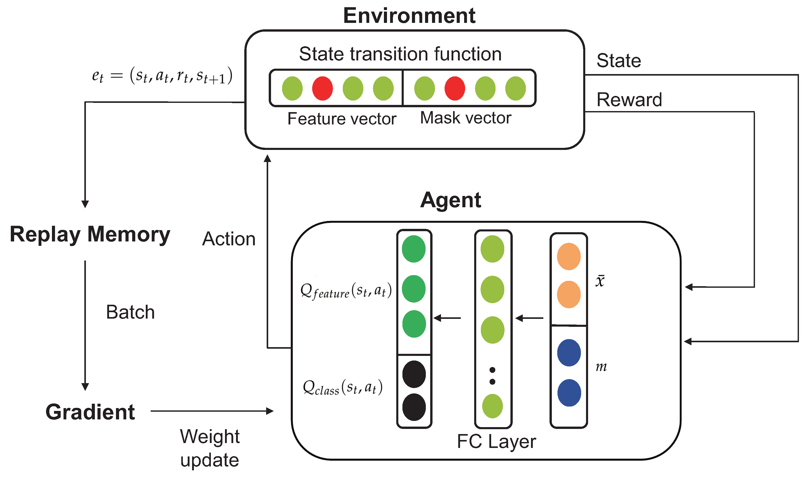
The previous section describes the basic concept of the deep Q-network. This section describes the implementation of the environment and training procedures. The POMDP environment was implemented with the deep Q-network algorithm, where the initial state was randomly drawn from the training dataset, and the observed state s consisted of (). For the neural network input, the observed state s was converted to the tuple , where is a mask vector of the original x that contains acquired feature values and m is a mask vector that denotes the acquired feature index [32]. The mask m consisted of . When the agent picked the ith feature, the mask vector was assigned the value of 1. The main purpose of the reinforcement learning model is to solve a sequential decision-making problem. Thus, the agent learned the optimal policy to find the optimal features from the feature set and classify the low level of vigilance and awake conditions. To find the optimal feature combinations among all features in an episode, the agent should not pick the same feature. This was realized by using a mask vector. The mask vector m contained the history of all agent actions in an episode. The vectors and m were given as follows:
The agent was designed to have the structure of a three-layer artificial neural network (ANN), where the input layer was the observed state and the output layer represented Q-values, including and . The overall learning procedure of the agent is illustrated in Figure 3.
The neural network that represents the Q-network had the inputs of the feature vector x and mask vector m. It was built from three fully connected layers with the ReLU activation function and an output layer with the linear function to produce the Q-value. The feature vector x had 22 dimensions, including the number of feature sets and the dimension of the mask vector m. Before the Q-network weight was updated, the replay memory should store enough episodes, where the agent selects a random action with the probability and stores its transition to the replay memory. Initially, 2000 transitions episodes were stored in the replay memory buffer. The environment initialized the initial state without any feature information. After enough transition data were accumulated in the replay memory, the Q-network was updated. When an episode was terminated, in Equation (5) was determined by the environment, where the target Q-network and soft target update methods were applied [29,51]. The target Q-values were constrained to changing slowly, which greatly improved the stability of the learning process. The weight of the target Q-network was kept to be updated. If the agent selected the ith feature in the feature set, the environment assigned the ith feature value to the feature vector x and assigned 1 to the ith component in the vector m. The training and environment simulation algorithm procedures are described in Algorithm 1.
For every time step, the agent interacted with the environment . In the action space , the agent selected the or action to classify the state or select a feature. When the agent chose the action, the environment added the chosen feature to the set of selected features and created the mask . By using the mask vector, the environment forced the agent to not choose the same action or feature by subtracting from the Q value. The environment simulation algorithm procedures are described in Algorithm 2.
To evaluate the classification performance of the reinforcement learning algorithm, the accuracy, precision, recall, and F1 score were calculated as follows:
where TP is a true positive, TN is a true negative, FN is a false negative, and TN is a true negative.
| Algorithm 1: Agent training. |
 |
| Algorithm 2: Environment.simulation. |
 |
3. Experimental Results
3.1. Classification for Assessment of Vigilance
The total EEG and ECG data were divided into five segments for the fivefold validation method [52]. Four segments were used as the training set, and the other segment was used as the test set. This process was repeated five times so that each segment could be the test set. The cost factor in Equation (1) was set to 0.05 because it yielded the best classification accuracy in this experiment. The accuracy was decreased when the cost factor was 0.1 and the number of selected features was increased when the cost factor was 0.01. The cost factor for maximum accuracy while minimizing the number of selected features was 0.05. If the value is high, the classification accuracy should be low, and the number of selected features should increase because the agent receives a negative reward for the feature selection action . During the training process, the -greedy policy was used; this was not applied during the validation and testing processes.
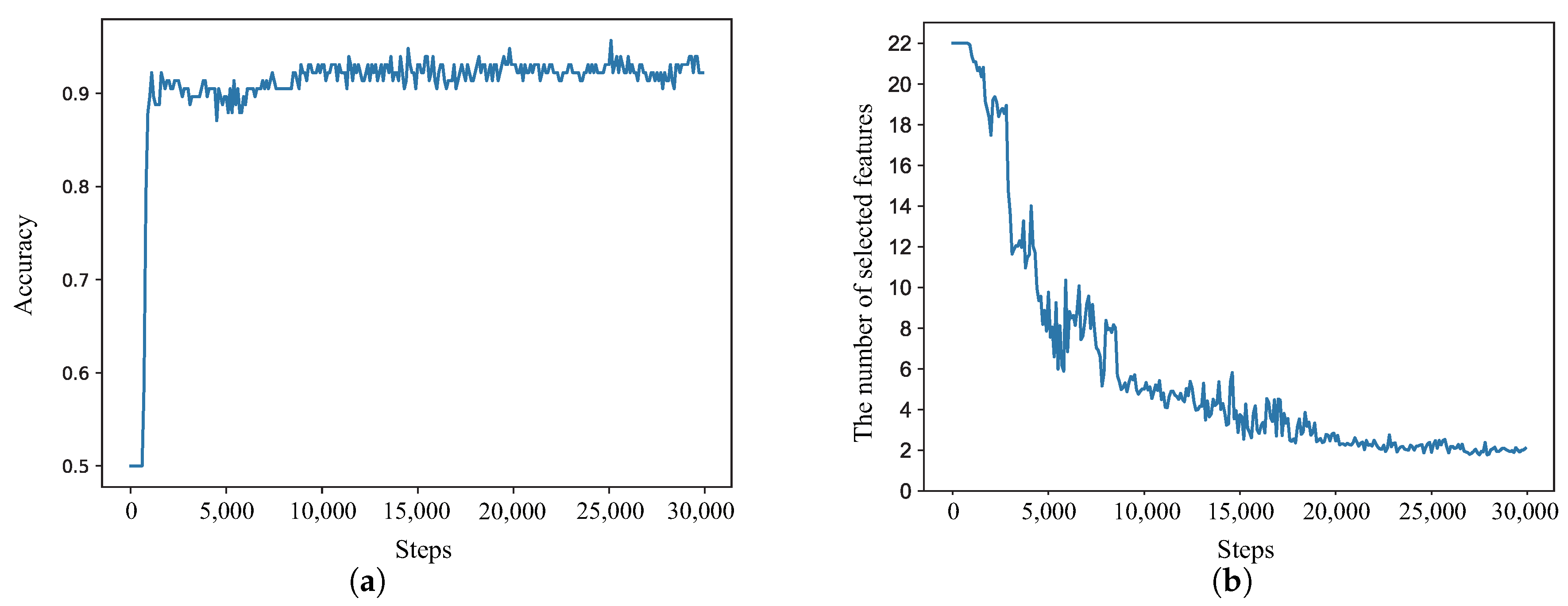
Figure 4 illustrates the accuracy of the deep Q-network (DQN) agent and the number of selected features. Figure 4a shows the DQN agent classification performance of subject 10, as the learning steps were increased during the training session, and Figure 4b illustrates the number of features chosen by the DQN agent. The means of the TP, TN, FP, and FN results across the five-fold cross-validation segments were calculated.
Table 3 presents the classification results of the 11 subjects. The DQN agent classification accuracy was more than 90%, although the results for Subjects 2 and 5 had an accuracy of less than 80%.
3.2. Comparison with Conventional Methods
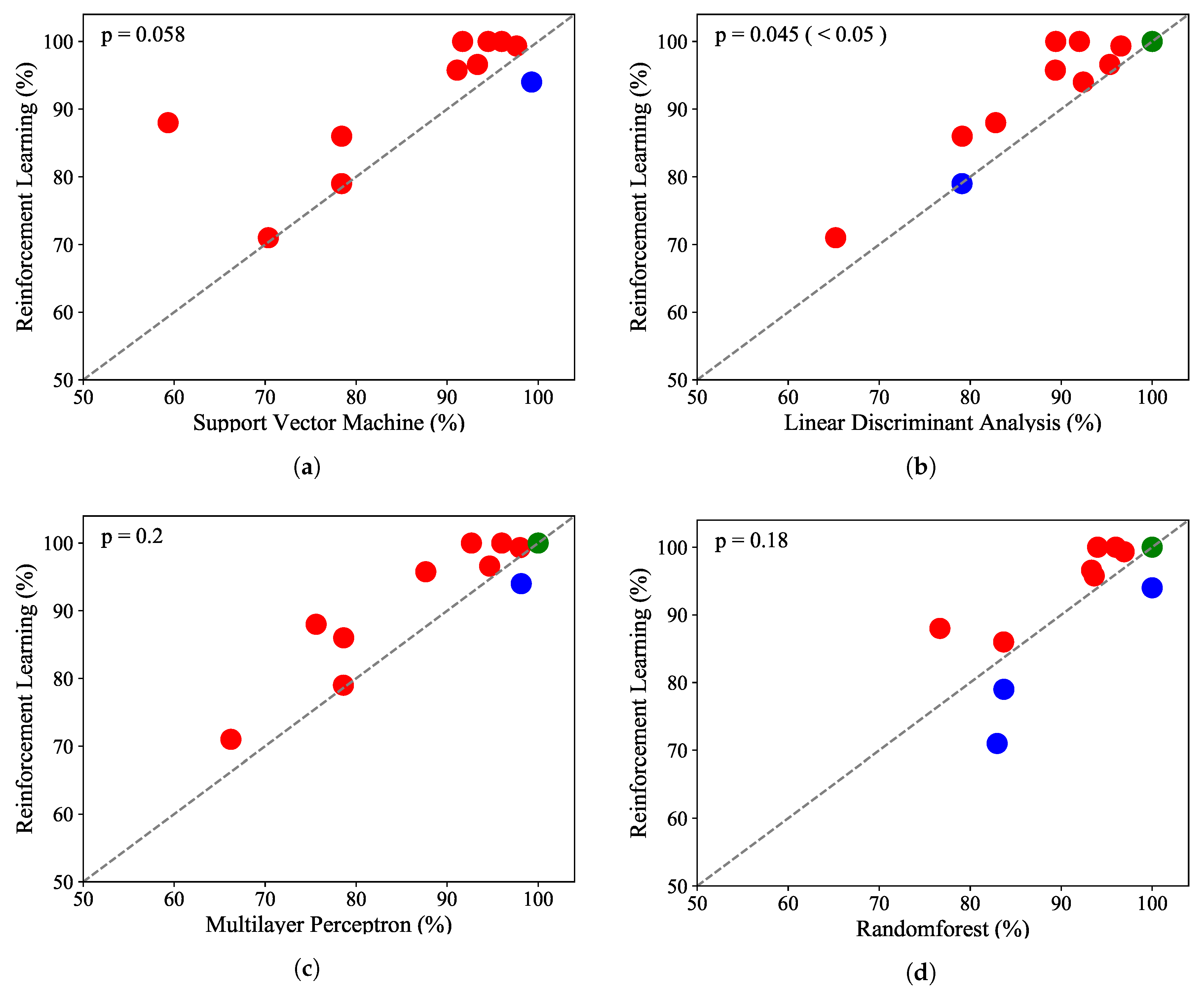
A benchmark test was performed to compare the reinforcement learning algorithm with several conventional supervised learning classifiers: linear discriminant analysis (LDA), the multilayer perceptron classifier (MLP), the support vector machine (SVM), and the random forest classifier. The LDA classifier is widely used for EEG classification problems [53] and finds a linear combination of features to separate different classes. The MLP is a basic deep learning model that optimizes the loss function by using gradient descent [45]. The SVM is a supervised learning method that is often used for regression and classification problems. With a kernel trick, an SVM can be used to solve both linear and nonlinear problems. Random forest is an ensemble machine learning algorithm that is widely used for physiological data analysis. Figure 5 compares the scatter plots of the reinforcement learning algorithm and conventional supervised learning algorithms.
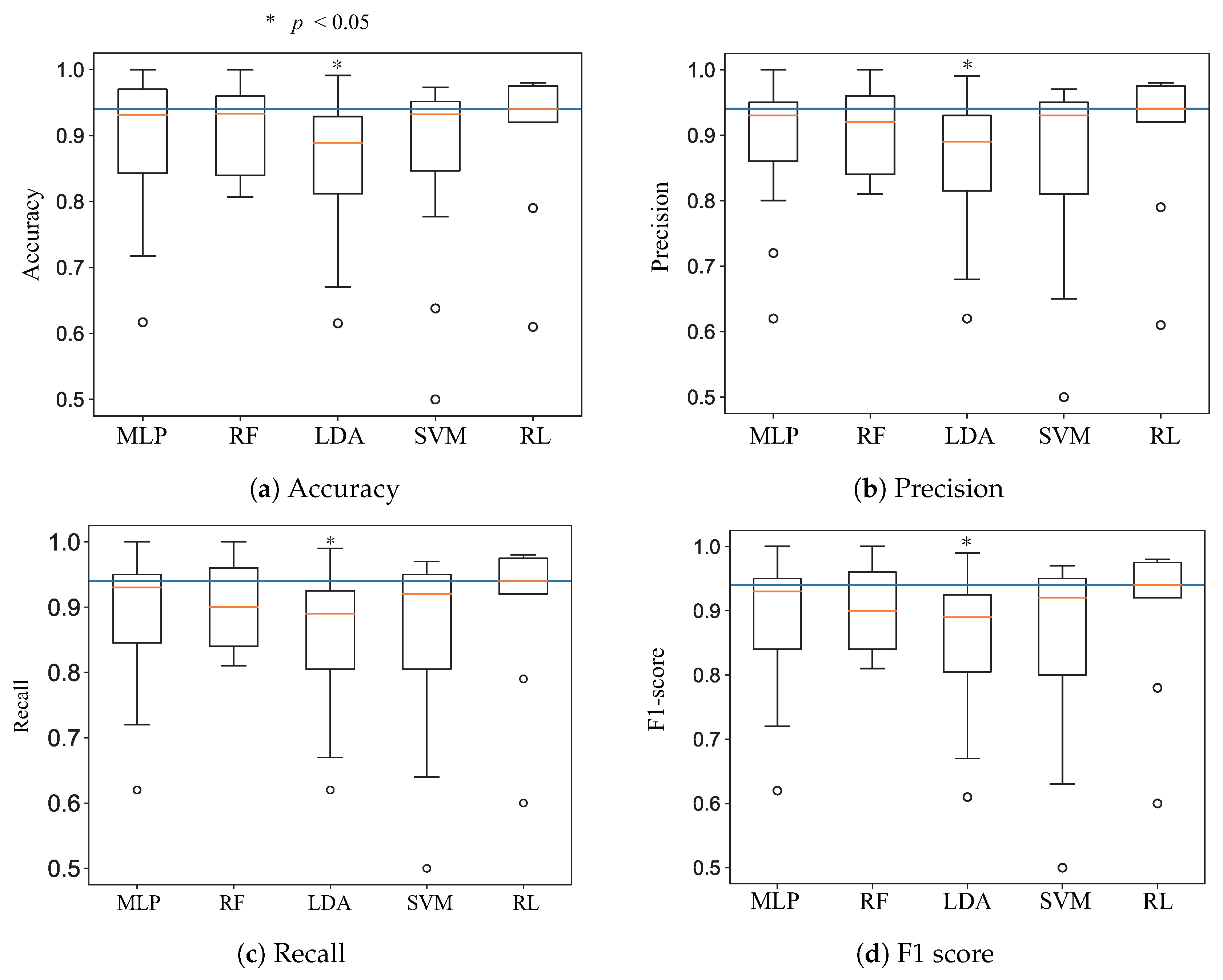
Each dot represents the classification accuracy of a subject; the red dots above the gray line indicate that the DQN agent had a higher classification accuracy than the other conventional supervised learning classifiers. The green dots indicate that the classification rates were the same, and the blue dots indicate that the DQN agent had lower accuracy than the conventional supervised learning classifiers. Figure 5a shows that the DQN agent yielded better accuracy than the SVM for 10 subjects, and the SVM was better for only one subject. MLP and LDA had better classification accuracy than the reinforcement learning algorithm for one subject, and the result was the same for one subject. The random forest showed the best performance among the conventional supervised learning classifiers; it had better accuracy for three subjects compared to the DQN agent. The Mann–Whitney rank test was performed to compare the accuracy, precision, recall, and F1 score values for the DQN agent with the others [54]. Figure 6 shows the p-values of the four cases. In particular, the reinforcement learning algorithm significantly outperformed LDA with a p-value of less than 0.05. Figure 7 illustrates that classification precision, recall, and F1 score values for the 11 subjects. The reinforcement learning (i.e., DQN) showed the best accuracy, precision, recall, and F1 score. Among the 11 subjects, two subjects had lower classification accuracies of 78% and 60%. Excluding these two outliers, the DQN agent showed a stable accuracy, precision, recall, and F1 score.
3.3. Feature Study
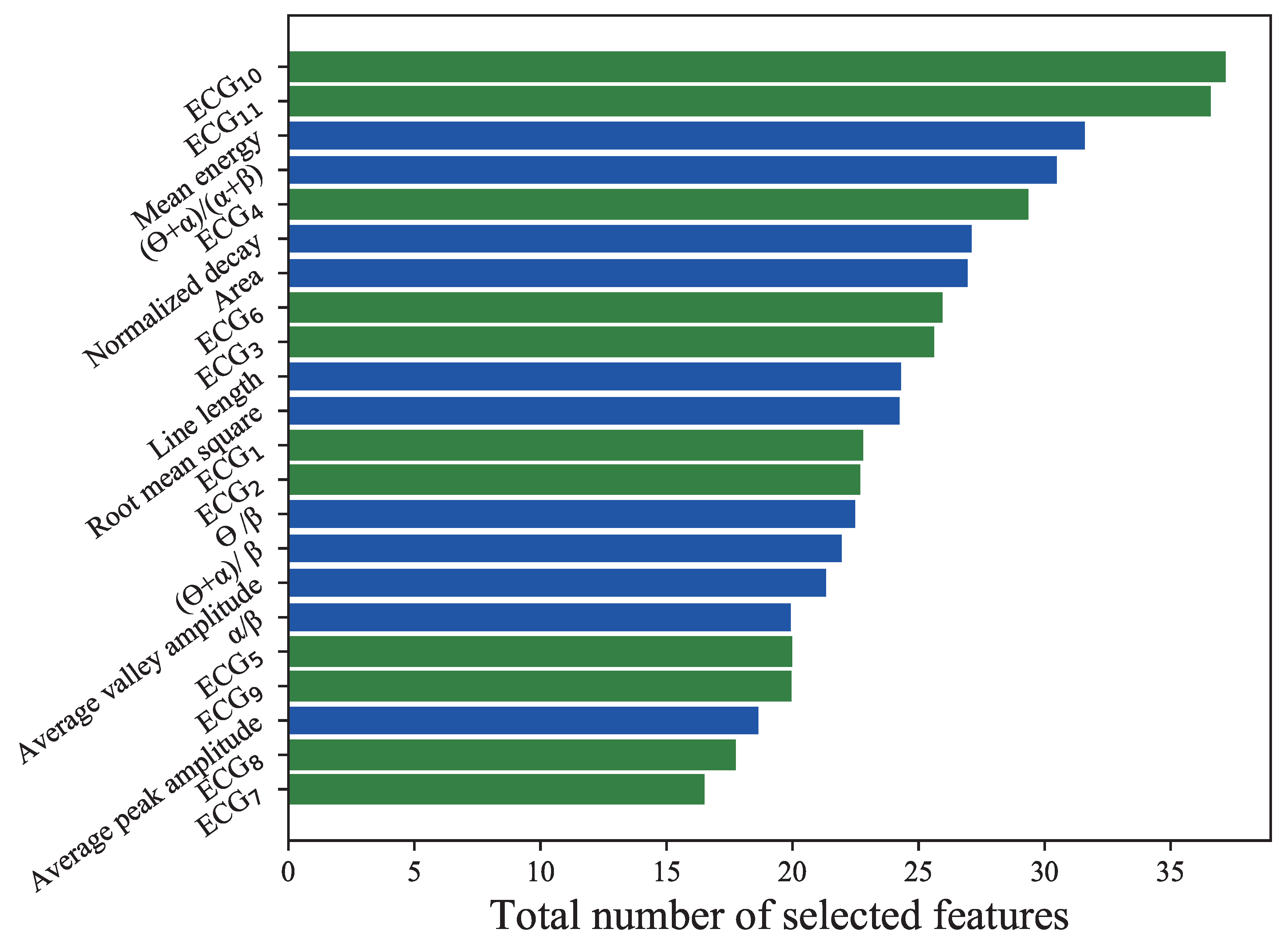
In order to investigate the significant features of the physiological response to the low level of vigilance state, the total feature set consisting of 11 EEG and 11 ECG features was fed to the DQN agent, which selected the best features for vigilance estimation. During the training process, the number of features selected by the DQN agent for all 11 subjects was counted, including all episodes during the fivefold cross-validation.
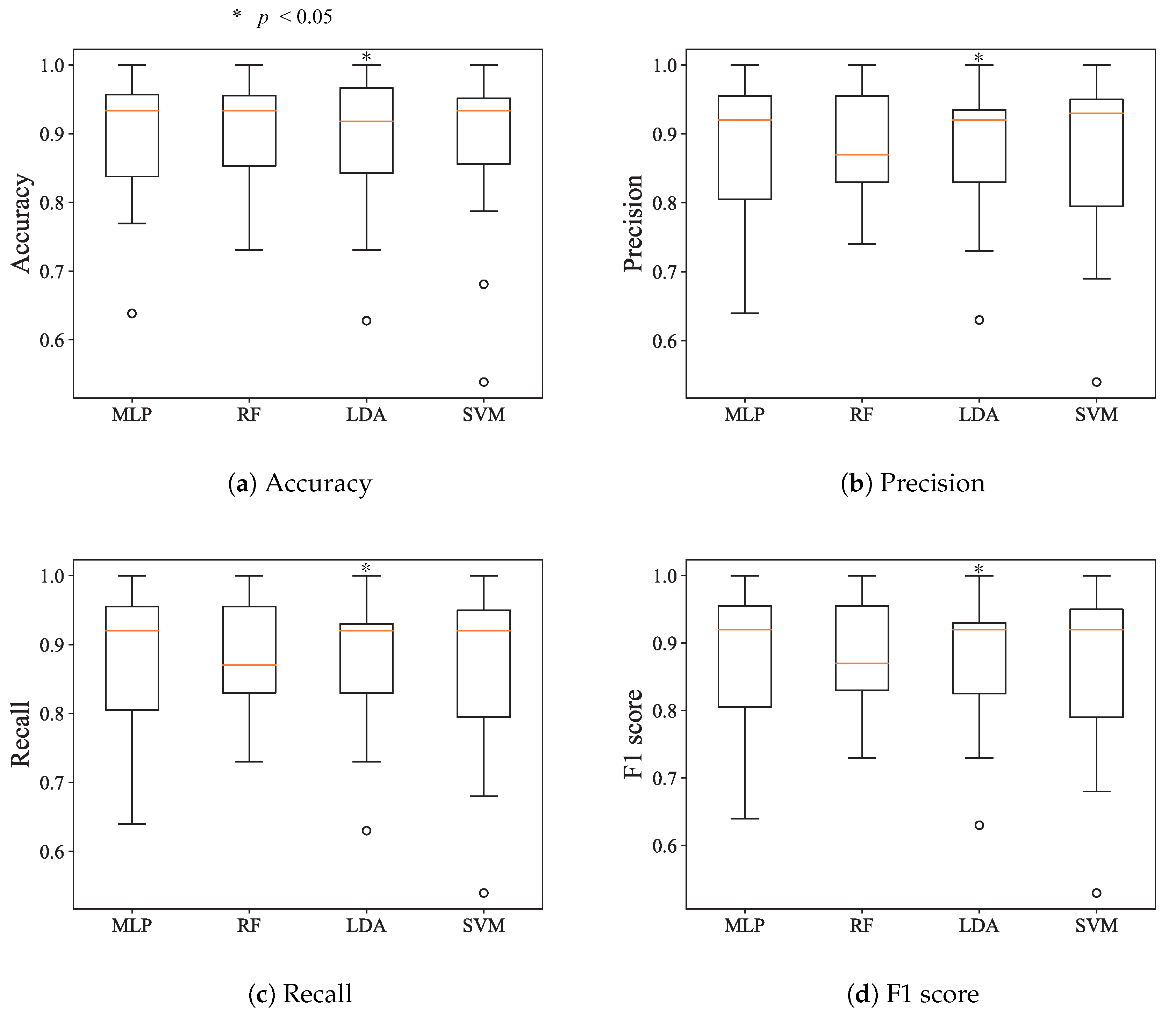
In Figure 7, the blue bars denote the total numbers of selected EEG features, and the green bars denote the total numbers of selected ECG features. In total, 268 EEG features and 273 ECG features were selected. On average, 2.48 EEG features (, standard deviation (SD)) and 2.45 ECG features (±1.134, SD) were selected. Among all ECG and EEG features, the 10th Deep-ECGNet feature and 11th ECG feature were selected most often. Among the EEG features, the mean energy was selected most often, followed by the frequency feature . In order to evaluate the significance of the selected features by the DQN agent, only some of the selected features were tested for the estimation of the vigilance state. Each episode represented trial data that were segmented into 10 s intervals. The DQN agent selected the best feature set for an episode based on its Q value, and the selected features were fed into the conventional classifiers. Because the DQN agent produced different Q values depending on the dataset of each subject, every subject had their own optimal feature set of two or three features. Figure 8a–d illustrates the box plots of the accuracy, precision, recall, and F1 score produced by the conventional classifiers with the optimal features. These results are comparable with those in Figure 7 obtained using all of the features, which suggests that using the DQN agent to select a few features could make the vigilance monitoring system lighter and more efficient by requiring fewer resources.
4. Discussion and Conclusions
A portable and wireless system was developed to monitor the low level of vigilance of a user. Because of the limited resources in terms of memory, processing, and battery power, optimizing the significant input or features is crucial to reducing the memory size and computation of the processor, and thus realizing low energy consumption. This study used the reinforcement algorithm of DQN to optimize the feature set of ECG and EEG responses to the state of low level vigilance. Figure 8 shows that selecting a feature set including only two or three features could yield a similar performance to that of using all of the features. This approach can be applied to most physiological and neuroscience research, where investigating the biomarkers for a physiological or cognitive condition is key to understanding the phenomenon. It was demonstrated that the reinforcement algorithm detects low level of vigilance using the optimized features more efficiently than conventional supervised learning classifiers, as shown in Figure 6 and Figure 8. In addition to the DQN used in this paper, asynchronous advantage actor critic (A3C), trust region policy optimization (TRPO), and proximal policy optimization (PPO) algorithms are utilized in the state-of-the-art reinforcement learning algorithm. For the optimization of the deep learning structure and parameters, neural architecture search (NAS) is widely used [27,55,56,57]. If the structure and the parameters of DQN are optimized through the NAS algorithm, the accuracy of the vigilance assessment will be increased. We left the parameter optimization and design of the new deep learning structure to future work. In this study, the DQN algorithm with the POMDP environment was applied to classify the low level of vigilance and optimize the feature set. The optimal feature selection process suggested that both ECG and EEG can be used to estimate the vigilance, although the two ECG features were selected more often, as shown in Figure 8. This implies that both the autonomous system (measured by ECG) and central nervous system (measured by EEG) are responsible for the drowsy condition, while the autonomous system has a slightly stronger influence. Thus, both ECG and EEG sensors should be used for the development of a vigilance state detection system. These results demonstrated that the deep learning approach of Deep-ECGNet can be a state-of-the-art algorithm for extracting features from a short-term ECG signal. This is supported by the results of Hwang et al. [25], who demonstrated its performance for monitoring stress in an experiment. Although the DQN agent uses few optimal features, it had a higher classification accuracy than conventional classifiers considered in this study (i.e., LDA, MLP, SVM, and random forest). DQN can also suggest significant features of EEG and ECG corresponding to a low level of vigilance, which can be used to investigate biomarkers for the physiological state.
Author Contributions
Conceptualization, W.S. and T.C.; methodology, W.S., H.L. and J.Y.; software, W.S. and M.Y.; formal analysis, W.S. and B.H.; investigation, M.Y. and H.L.; writing—original draft preparation, W.S.; writing—review and editing, W.S. and C.P.; All authors have read and agreed to the published version of the manuscript.
Funding
This research was supported by Basic Science Research Program through the National Research Foundation of Korea(NRF) funded by the Ministry of Science and ICT(NRF-2017R1A5A1015596) and the Research Grant of Kwangwoon University in 2020.
Conflicts of Interest
The authors declare no conflict of interest.
References
- Sahayadhas, A.; Sundaraj, K.; Murugappan, M. Detecting driver drowsiness based on sensors: A review. Sensors 2012, 12, 16937–16953. [Google Scholar] [CrossRef] [PubMed] [Green Version]
- Zhang, C.; Wu, X.; Zheng, X.; Yu, S. Driver drowsiness detection using multi-channel second order blind identifications. IEEE Access 2019, 7, 11829–11843. [Google Scholar] [CrossRef]
- Duta, M.; Alford, C.; Wilson, S.; Tarassenko, L. Neural network analysis of the mastoid EEG for the assessment of vigilance. Int. J. Hum.-Comput. Interact. 2004, 17, 171–195. [Google Scholar] [CrossRef]
- Shen, K.Q.; Li, X.P.; Ong, C.J.; Shao, S.Y.; Wilder-Smith, E.P. EEG-based mental fatigue measurement using multi-class support vector machines with confidence estimate. Clin. Neurophysiol. 2008, 119, 1524–1533. [Google Scholar] [CrossRef]
- Looney, D.; Kidmose, P.; Park, C.; Ungstrup, M.; Rank, M.L.; Rosenkranz, K.; Mandic, D.P. The in-the-ear recording concept: User-centered and wearable brain monitoring. IEEE Pulse 2012, 3, 32–42. [Google Scholar] [CrossRef]
- Akin, M.; Kurt, M.B.; Sezgin, N.; Bayram, M. Estimating vigilance level by using EEG and EMG signals. Neural Comput. Appl. 2008, 17, 227–236. [Google Scholar] [CrossRef]
- Åkerstedt, T.; Gillberg, M. Subjective and objective sleepiness in the active individual. Int. J. Neurosci. 1990, 52, 29–37. [Google Scholar] [CrossRef]
- Van Benthem, K.; Cebulski, S.; Herdman, C.M.; Keillor, J. An EEG Brain–Computer Interface Approach for Classifying Vigilance States in Humans: A Gamma Band Focus Supports Low Misclassification Rates. Int. J. Hum.- Interact. 2018, 34, 226–237. [Google Scholar] [CrossRef]
- Atkinson, J.; Campos, D. Improving BCI-based emotion recognition by combining EEG feature selection and kernel classifiers. Expert Syst. Appl. 2016, 47, 35–41. [Google Scholar] [CrossRef]
- Turner, J.; Page, A.; Mohsenin, T.; Oates, T. Deep belief networks used on high resolution multichannel electroencephalography data for seizure detection. In Proceedings of the 2014 AAAI Spring Symposium, Palo Alto, CA, USA, 24–26 March 2014. [Google Scholar]
- Forsman, P.M.; Vila, B.J.; Short, R.A.; Mott, C.G.; Van Dongen, H.P. Efficient driver drowsiness detection at moderate levels of drowsiness. Accid. Anal. Prev. 2013, 50, 341–350. [Google Scholar] [CrossRef]
- Britton, J.W.; Frey, L.C.; Hopp, J.; Korb, P.; Koubeissi, M.; Lievens, W.; Pestana-Knight, E.; St, E.L. Electroencephalography (EEG): An Introductory Text and Atlas of Normal and Abnormal Findings in Adults, Children, and Infants; American Epilepsy Society: Chicago, IL, USA, 2016. [Google Scholar]
- Jap, B.T.; Lal, S.; Fischer, P.; Bekiaris, E. Using EEG spectral components to assess algorithms for detecting fatigue. Expert Syst. Appl. 2009, 36, 2352–2359. [Google Scholar] [CrossRef]
- Åkerstedt, T.; Kecklund, G.; Knutsson, A. Manifest sleepiness and the spectral content of the EEG during shift work. Sleep 1991, 14, 221–225. [Google Scholar] [CrossRef] [PubMed]
- Acharya, U.R.; Fujita, H.; Oh, S.L.; Hagiwara, Y.; Tan, J.H.; Adam, M. Application of deep convolutional neural network for automated detection of myocardial infarction using ECG signals. Inf. Sci. 2017, 415, 190–198. [Google Scholar] [CrossRef]
- Tan, J.H.; Hagiwara, Y.; Pang, W.; Lim, I.; Oh, S.L.; Adam, M.; San Tan, R.; Chen, M.; Acharya, U.R. Application of stacked convolutional and long short-term memory network for accurate identification of CAD ECG signals. Comput. Biol. Med. 2018, 94, 19–26. [Google Scholar] [CrossRef] [PubMed]
- Park, E.; Lee, J. A Computer-aided, Automatic Heart Disease-detection System with Dry-electrode-based Outdoor Shirts. IEIE Trans. Smart Process. Comput. 2019, 8, 8–13. [Google Scholar] [CrossRef]
- Chui, K.T.; Tsang, K.F.; Chi, H.R.; Ling, B.W.K.; Wu, C.K. An accurate ECG-based transportation safety drowsiness detection scheme. IEEE Trans. Ind. Inform. 2016, 12, 1438–1452. [Google Scholar] [CrossRef]
- Sahayadhas, A.; Sundaraj, K.; Murugappan, M. Drowsiness detection during different times of day using multiple features. Australas. Phys. Eng. Sci. Med. 2013, 36, 243–250. [Google Scholar] [CrossRef]
- Mansour, R.F. Deep-learning-based automatic computer-aided diagnosis system for diabetic retinopathy. Biomed. Eng. Lett. 2018, 8, 41–57. [Google Scholar] [CrossRef]
- Beritelli, F.; Capizzi, G.; Lo Sciuto, G.; Napoli, C.; Scaglione, F. Automatic heart activity diagnosis based on Gram polynomials and probabilistic neural networks. Biomed. Eng. Lett. 2018, 8, 77–85. [Google Scholar] [CrossRef]
- Wei, R.; Zhang, X.; Wang, J.; Dang, X. The research of sleep staging based on single-lead electrocardiogram and deep neural network. Biomed. Eng. Lett. 2018, 8, 87–93. [Google Scholar] [CrossRef]
- Piryatinska, A.; Terdik, G.; Woyczynski, W.A.; Loparo, K.A.; Scher, M.S.; Zlotnik, A. Automated detection of neonate EEG sleep stages. Comput. Methods Programs Biomed. 2009, 95, 31–46. [Google Scholar] [CrossRef] [PubMed]
- Goldberger, A.L.; Amaral, L.A.; Glass, L.; Hausdorff, J.M.; Ivanov, P.C.; Mark, R.G.; Mietus, J.E.; Moody, G.B.; Peng, C.K.; Stanley, H.E. PhysioBank, PhysioToolkit, and PhysioNet: Components of a new research resource for complex physiologic signals. Circulation 2000, 101, e215–e220. [Google Scholar] [CrossRef] [Green Version]
- Hwang, B.; You, J.; Vaessen, T.; Myin-Germeys, I.; Park, C.; Zhang, B.T. Deep ECGNet: An optimal deep learning framework for monitoring mental stress using ultra short-term ECG signals. Telemed. e-Health 2018, 24, 753–772. [Google Scholar] [CrossRef]
- Gunning, D. Explainable Artificial Intelligence (xai); Defense Advanced Research Projects Agency (DARPA): Arlington County, VA, USA, 2017; Volume 2.
- Zoph, B.; Le, Q.V. Neural architecture search with reinforcement learning. arXiv 2016, arXiv:1611.01578. [Google Scholar]
- Mnih, V.; Kavukcuoglu, K.; Silver, D.; Graves, A.; Antonoglou, I.; Wierstra, D.; Riedmiller, M. Playing atari with deep reinforcement learning. arXiv 2013, arXiv:1312.5602. [Google Scholar]
- Mnih, V.; Kavukcuoglu, K.; Silver, D.; Rusu, A.A.; Veness, J.; Bellemare, M.G.; Graves, A.; Riedmiller, M.; Fidjeland, A.K.; Ostrovski, G.; et al. Human-level control through deep reinforcement learning. Nature 2015, 518, 529. [Google Scholar] [CrossRef] [PubMed]
- Massoz, Q.; Langohr, T.; François, C.; Verly, J.G. The ULg multimodality drowsiness database (called DROZY) and examples of use. In Proceedings of the 2016 IEEE Winter Conference on Applications of Computer Vision (WACV), Lake Placid, NY, USA, 7–9 March 2016; pp. 1–7. [Google Scholar]
- Lee, H.; Lee, J.; Shin, M. Using Wearable ECG/PPG Sensors for Driver Drowsiness Detection Based on Distinguishable Pattern of Recurrence Plots. Electronics 2019, 8, 192. [Google Scholar] [CrossRef] [Green Version]
- Janisch, J.; Pevnỳ, T.; Lisỳ, V. Classification with Costly Features using Deep Reinforcement Learning. arXiv 2017, arXiv:1711.07364. [Google Scholar] [CrossRef] [Green Version]
- Janisch, J.; Pevnỳ, T.; Lisỳ, V. Classification with Costly Features as a Sequential Decision-Making Problem. arXiv 2019, arXiv:1909.02564. [Google Scholar]
- Chen, Y.E.; Tang, K.F.; Peng, Y.S.; Chang, E.Y. Effective Medical Test Suggestions Using Deep Reinforcement Learning. arXiv 2019, arXiv:1905.12916. [Google Scholar]
- Yamagata, T.; Santos-Rodríguez, R.; McConville, R.; Elsts, A. Online Feature Selection for Activity Recognition using Reinforcement Learning with Multiple Feedback. arXiv 2019, arXiv:1908.06134. [Google Scholar]
- Peng, Y.S.; Tang, K.F.; Lin, H.T.; Chang, E. Refuel: Exploring sparse features in deep reinforcement learning for fast disease diagnosis. In Advances in Neural Information Processing Systems; The MIT Press: Cambridge, MA, USA, 2018; pp. 7322–7331. [Google Scholar]
- Seok, W.; Park, C. Recognition of Human Motion with Deep Reinforcement Learning. IEIE Trans. Smart Process. Comput. 2018, 7, 245–250. [Google Scholar] [CrossRef]
- Rapaport, E.; Shriki, O.; Puzis, R. EEGNAS: Neural Architecture Search for Electroencephalography Data Analysis and Decoding. In Proceedings of the International Workshop on Human Brain and Artificial Intelligence, Macao, China, 12 August 2019; pp. 3–20. [Google Scholar]
- Klem, G.H.; Lüders, H.O.; Jasper, H.; Elger, C. The ten-twenty electrode system of the International Federation. Electroencephalogr. Clin. Neurophysiol. 1999, 52, 3–6. [Google Scholar]
- Selesnick, I.W.; Burrus, C.S. Generalized digital Butterworth filter design. IEEE Trans. Signal Process. 1998, 46, 1688–1694. [Google Scholar] [CrossRef] [Green Version]
- Correa, A.G.; Orosco, L.; Laciar, E. Automatic detection of drowsiness in EEG records based on multimodal analysis. Med. Eng. Phys. 2014, 36, 244–249. [Google Scholar] [CrossRef]
- Srivastava, N.; Hinton, G.; Krizhevsky, A.; Sutskever, I.; Salakhutdinov, R. Dropout: A simple way to prevent neural networks from overfitting. J. Mach. Learn. Res. 2014, 15, 1929–1958. [Google Scholar]
- Caruana, R.; Lawrence, S.; Giles, C.L. Overfitting in neural nets: Backpropagation, conjugate gradient, and early stopping. In Advances in Neural Information Processing Systems; The MIT Press: Cambridge, MA, USA, 2001; pp. 402–408. [Google Scholar]
- Sak, H.; Senior, A.; Beaufays, F. Long short-term memory recurrent neural network architectures for large scale acoustic modeling. In Proceedings of the Fifteenth Annual Conference of the International Speech Communication Association, Singapore, 14–18 September 2014. [Google Scholar]
- Gardner, M.W.; Dorling, S. Artificial neural networks (the multilayer perceptron)—A review of applications in the atmospheric sciences. Atmos. Environ. 1998, 32, 2627–2636. [Google Scholar] [CrossRef]
- Puterman, M.L. Markov Decision Processes: Discrete Stochastic Dynamic Programming; John Wiley & Sons: Hoboken, NJ, USA, 2014. [Google Scholar]
- Sutton, R.S.; Barto, A.G. Introduction to Reinforcement Learning; MIT Press: Cambridge, MA, USA, 1998; Volume 135. [Google Scholar]
- Kaelbling, L.P.; Littman, M.L.; Cassandra, A.R. Planning and acting in partially observable stochastic domains. Artif. Intell. 1998, 101, 99–134. [Google Scholar] [CrossRef] [Green Version]
- Silver, D.; Huang, A.; Maddison, C.J.; Guez, A.; Sifre, L.; Van Den Driessche, G.; Schrittwieser, J.; Antonoglou, I.; Panneershelvam, V.; Lanctot, M.; et al. Mastering the game of Go with deep neural networks and tree search. Nature 2016, 529, 484. [Google Scholar] [CrossRef]
- Lin, L.J. Reinforcement Learning for Robots Using Neural Networks; Technical Report; Carnegie-Mellon Univ Pittsburgh PA School of Computer Science: Pittsburgh, PA, USA, 1993. [Google Scholar]
- Lillicrap, T.P.; Hunt, J.J.; Pritzel, A.; Heess, N.; Erez, T.; Tassa, Y.; Silver, D.; Wierstra, D. Continuous control with deep reinforcement learning. arXiv 2015, arXiv:1509.02971. [Google Scholar]
- Bengio, Y.; Grandvalet, Y. No unbiased estimator of the variance of k-fold cross-validation. J. Mach. Learn. Res. 2004, 5, 1089–1105. [Google Scholar]
- Zhou, W.; Liu, Y.; Yuan, Q.; Li, X. Epileptic seizure detection using lacunarity and Bayesian linear discriminant analysis in intracranial EEG. IEEE Trans. Biomed. Eng. 2013, 60, 3375–3381. [Google Scholar] [CrossRef] [PubMed]
- Ruxton, G.D. The unequal variance t-test is an underused alternative to Student’s t-test and the Mann–Whitney U test. Behav. Ecol. 2006, 17, 688–690. [Google Scholar] [CrossRef]
- Schulman, J.; Levine, S.; Abbeel, P.; Jordan, M.; Moritz, P. Trust region policy optimization. In Proceedings of the International Conference on Machine Learning, Lille, France, 6–11 July 2015; pp. 1889–1897. [Google Scholar]
- Schulman, J.; Wolski, F.; Dhariwal, P.; Radford, A.; Klimov, O. Proximal policy optimization algorithms. arXiv 2017, arXiv:1707.06347. [Google Scholar]
- Mnih, V.; Badia, A.P.; Mirza, M.; Graves, A.; Lillicrap, T.; Harley, T.; Silver, D.; Kavukcuoglu, K. Asynchronous methods for deep reinforcement learning. In Proceedings of the International Conference on Machine Learning, New York City, NY, USA, 19–24 June 2016; pp. 1928–1937. [Google Scholar]
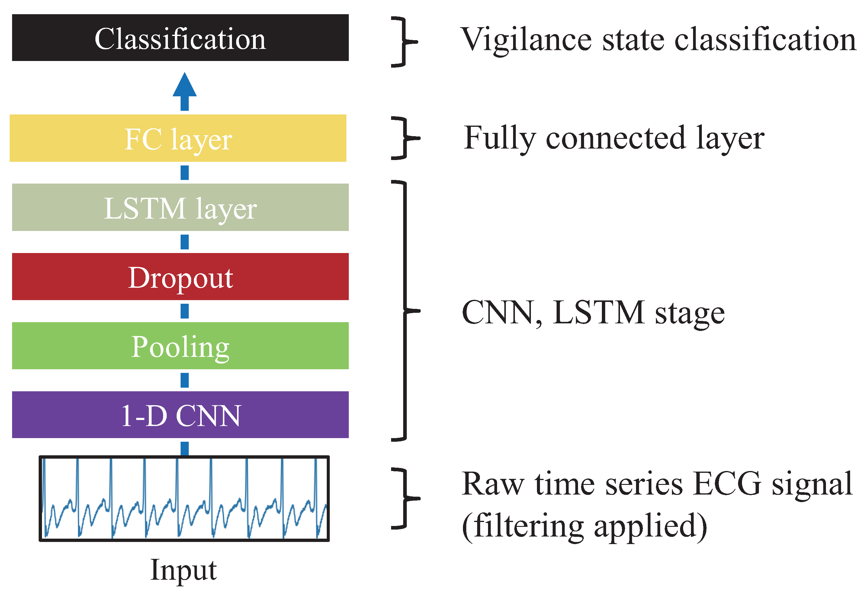
Figure 1.
Deep- ECGNet model structure, which consists of a 1D CNN, LSTM, and fully connected layer for extracting electrocardiogram (ECG) features.
Figure 1.
Deep- ECGNet model structure, which consists of a 1D CNN, LSTM, and fully connected layer for extracting electrocardiogram (ECG) features.

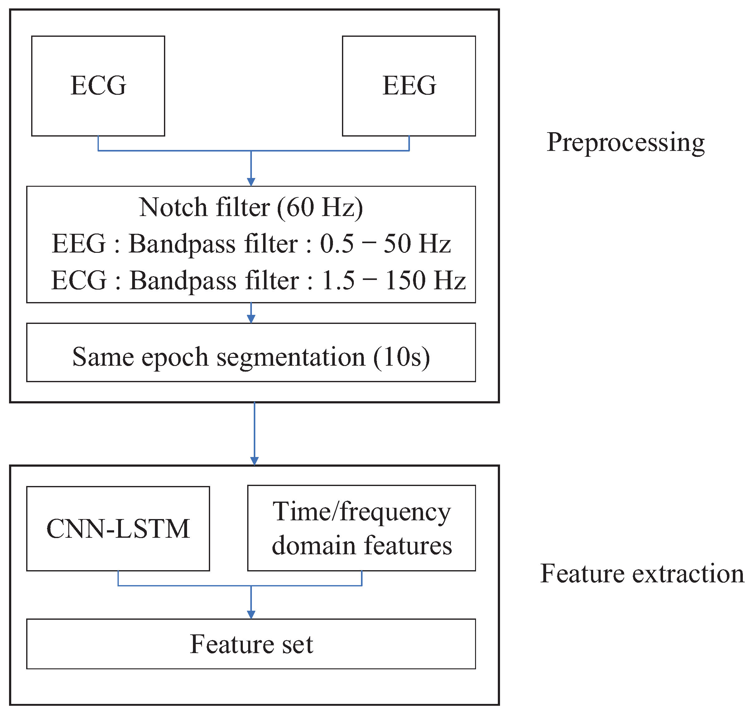
Figure 2.
Feature extraction with electroencephalogram (EEG) and ECG signals.

Figure 3.
Procedure for extracting features from EEG and ECG signals with the reinforcement learning algorithm.
Figure 3.
Procedure for extracting features from EEG and ECG signals with the reinforcement learning algorithm.

Figure 4.
Deep Q-network (DQN) agent classification results as the learning steps during the training session and number of features used for subject 10 were increased. (a) Classification results with the deep reinforcement learning agent; (b) number of selected features.
Figure 4.
Deep Q-network (DQN) agent classification results as the learning steps during the training session and number of features used for subject 10 were increased. (a) Classification results with the deep reinforcement learning agent; (b) number of selected features.

Figure 5.
Scatter plots for the classification results of the 11 subjects compared with the results of conventional classifiers. (a) scatterplot of the classification rates comparing RL classifier with SVM; (b)scatterplot of the classification rates comparing RL classifier with LDA; (c) scatterplot of the classification rates comparing RL classifier with MLP; (d) scatterplot of the classification rates comparing RL classifier with RF;

Figure 6.
Boxplots of the accuracy, precision, recall, and F1 score based on the classification results of the 11-subject dataset.
Figure 6.
Boxplots of the accuracy, precision, recall, and F1 score based on the classification results of the 11-subject dataset.

Figure 7.
Total number of selected features by the DQN agent for all 11 subjects. Green bars represent the results of the 11 ECG features extracted with deep-ECGNet, and blue bars illustrate those of the 11 EEG features extracted by conventional feature engineering. denotes the ECG features extracted using DeepECGNet.

Figure 8.
Boxplots of the accuracy, precision, recall, and F1 score using the features selected by the DQN agent.
Figure 8.
Boxplots of the accuracy, precision, recall, and F1 score using the features selected by the DQN agent.


Table 1.
Time-domain features of the EEG signal.
| Feature | Equation |
|---|---|
| Area | A = |
| Normalized decay | |
| Line length | |
| Mean energy | |
| Root mean square | |
| Average peak amplitude | |
| Average valley amplitude |
Table 2.
An overview of CNN and LSTM architecture details.
| Layers | Configurations |
|---|---|
| Convolution Layer | 1D conv, input channel : 1, output channel : 128, kernel size : 1000 |
| Pooling Layer | Max pool : 800, stride : 1 |
| LSTM Layer | Input channel : 128, hidden : 32, number of recurrent layers : 2 |
| Fully connected Layer | Input channel : 352, output : 22 |
| Classification Layer | Input channel : 22, output : 2 |
Table 3.
Classification accuracy, precision, recall, and F1 score values for 11 subjects produced by the DQN agent.
Table 3.
Classification accuracy, precision, recall, and F1 score values for 11 subjects produced by the DQN agent.
| Subject | Accuracy | Precision | Recall | F1 Score |
|---|---|---|---|---|
| 1 | 0.98 | 0.98 | 0.98 | 0.98 |
| 2 | 0.79 | 0.79 | 0.79 | 0.78 |
| 3 | 0.95 | 0.95 | 0.95 | 0.95 |
| 4 | 0.98 | 0.98 | 0.98 | 0.98 |
| 5 | 0.6 | 0.61 | 0.6 | 0.6 |
| 6 | 0.92 | 0.92 | 0.92 | 0.92 |
| 7 | 0.98 | 0.98 | 0.98 | 0.98 |
| 8 | 0.92 | 0.92 | 0.92 | 0.92 |
| 9 | 0.94 | 0.94 | 0.94 | 0.94 |
| 10 | 0.97 | 0.97 | 0.97 | 0.97 |
| 11 | 0.93 | 0.93 | 0.93 | 0.93 |
© 2020 by the authors. Licensee MDPI, Basel, Switzerland. This article is an open access article distributed under the terms and conditions of the Creative Commons Attribution (CC BY) license (http://creativecommons.org/licenses/by/4.0/).
Share and Cite
MDPI and ACS Style
Seok, W.; Yeo, M.; You, J.; Lee, H.; Cho, T.; Hwang, B.; Park, C. Optimal Feature Search for Vigilance Estimation Using Deep Reinforcement Learning. Electronics 2020, 9, 142. https://doi.org/10.3390/electronics9010142
AMA Style
Seok W, Yeo M, You J, Lee H, Cho T, Hwang B, Park C. Optimal Feature Search for Vigilance Estimation Using Deep Reinforcement Learning. Electronics. 2020; 9(1):142. https://doi.org/10.3390/electronics9010142
Chicago/Turabian StyleSeok, Woojoon, Minsoo Yeo, Jiwoo You, Heejun Lee, Taeheum Cho, Bosun Hwang, and Cheolsoo Park. 2020. "Optimal Feature Search for Vigilance Estimation Using Deep Reinforcement Learning" Electronics 9, no. 1: 142. https://doi.org/10.3390/electronics9010142
Note that from the first issue of 2016, this journal uses article numbers instead of page numbers. See further details here.