A Transient Modeling of the Thermoelectric Generators for Application in Wireless Sensor Network Nodes

Abstract

This paper reports results of the transient modeling of thermoelectric cooling/heating modules as power generators with the aim to select preferable ones for use in thermal energy harvesting wireless sensor network nodes. A study is conducted using the selected commercial thermoelectric generators within the node of a compact design with aluminum PCBs. Their equivalent electro-thermal models suitable for SPICE-like simulators are presented. Model components are extracted from the geometrical, physical and thermo-electrical parameters and/or experimentally. SPICE simulation results mismatch within 7% in comparison with the experimental measurements. The presented model is used for the characterization of different thermoelectric generators within the wireless sensor network node from the aspects of harvesting efficiency, cold boot time, node dimensions and compactness, and maximum applicable temperature. The choice of the preferred generator is determined by its electrical resistance, the number of thermoelectric pairs, external area and thermoelectric legs length, depending on the primary design goal and imposed thermal operating conditions. The node can provide load power of 1.3 $\mathrm{m}\mathrm{W}$ and the cold boot time of 66 s for generator with 31 thermoelectric pairs at a temperature difference of 15 $°\mathrm{C}$ with respect to the ambient, and 7.6 $\mathrm{m}\mathrm{W}$ of load power and the cold boot time of 40 s for generator with 71 thermoelectric pairs at a temperature difference of 25 $°\mathrm{C}$.

1. Introduction

The wireless sensor network (WSN) nodes, combining processor with sensors and transceiver, record and transmit specific data to either a central point or other peer nodes on the network. These nodes tend to have low duty cycles, low-power sleep states, and relatively high power “on” states when sending and receiving data. Numerous applications of wireless sensor networks have focused on medical, environmental, automotive and industrial monitoring that requires a long service life. This orients designers to move powering of the nodes beyond batteries into the energy harvesting domain [1]. Therefore, nodes are often powered by harvesting thermal, light, mechanical or electromagnetic radiation energy from the ambient in an independent or joint manner [2,3,4,5,6,7]. Temperature gradients and heat flow are usually present in nature and offer the opportunity to transform thermal energy from the environment into the electricity. Versatile thermoelectric generators (TEGs) are commonly exploited for this type of energy conversion. Also, conventional thermoelectric cooling/heating modules have successfully been applied as thermoelectric generators for powering wireless sensor network nodes [8,9,10].

TEGs are solid-state devices without moving parts. They are silent, reliable and scalable, which makes them ideal for small, distributed power generation systems and energy harvesting [11,12]. Although their energy conversion efficiency is relatively low (typically 5–8%), these devices are widely applied for waste heat recovery. Conventional TEGs contain many thermoelectric pairs made of n-type and p-type thermoelectric legs connected by copper electrodes electrically in series and thermally in parallel. These legs are positioned between two thin and thermally high conductive alumina ceramic plates. In order to design high-efficiency TEG based energy harvesting systems, their accurate electro-thermal models must be employed. In general, the models contain R or RC circuits to represent thermal resistance and thermal mass of TEGs. Therefore, some of the models are steady-state [8,13,14,15], while the others are transient [16,17,18,19,20]. In [16], a comparison of experimental and SPICE modeled time-domain response of the thermoelectric cooler is presented. The results are given for the scenario where the temperature difference between the sides of the TEG has been established and then the time-domain relaxation has been observed by measuring the generated voltage. Transient SPICE model derived from one-dimensional heat transfer differential equations is presented in [17]. The proposed model enables calculation of the temperature profile inside the TEG by taking into account the real temperature dependences of the material properties. This is essential in the simulation of the TEG exposed to a large temperature difference.

In [15], contact resistances between the TEG elements are determined by non-linear regression analysis based on the results from 3D finite element simulations and experimental measurement of the heat flow, voltage and current. Research presented in [21] is focused on the determination of the parasitic reactive elements that appear in the TEG by the phase offset measurement using an oscilloscope. The effective internal resistance of TEG can vary from its specified electrical resistance value due to the mutual dependence of the electrical and thermal effects. Accordingly, in [22], a systematic method for accurate determination of the TEG internal resistance is developed. An important feature of the model presented in [23] is its ability to generate small signal transfer functions that can be used to design a feedback network in the temperature control applications. Some authors used the manufacturer’s datasheet parameters to build their own models while others combined them with experimentally obtained parameters [22,23,24,25,26]. A methodology for extraction of the temperature-dependent parameters of a TEG by the voltage, current and temperature measurements is presented in [27]. The SPICE TEG models for LED driver, self-powered wearable electronic devices and sanitary applications are presented in [28,29,30]. The nonlinear heat diffusion equations in TEG are solved and the lumped parameter electrical model is proposed in [31]. The equivalent electrical circuit presented in [32] includes a diode in parallel to the electrical resistance of the TEG to simulate current-dependent resistance.

In [32,33,34,35,36], the authors have investigated the equivalent circuits of the energy conversion processes in thermoelectric modules/generators. These models are used in a conjunction with the equivalent thermal elements representing other building blocks of the system and characteristics of the electrical loading for quick estimation of the WSN node performances. The contributions of the Seebeck, Joule and Peltier effect to the generated voltage and the heat rates absorbed or released at the junctions of the TEG are included in SPICE models via controlled voltage and current sources. Overall, equivalent circuits developed for SPICE-like simulators presented in [28,29,30] often can be used for the design of the complex systems in a simpler way then analytical models proposed in [31,37,38].

The models presented in the literature did not consider the behavior of cooling/heating modules when used as a thermoelectric generator inside the complex system in the time domain. In previous works [9,13], we have shown how TEG behaves inside the WSN node in the steady–state, when the temperature difference is fixed. In this paper, we extend the analysis to the transient regime, with the development of the appropriate SPICE model. Thermal capacitances are introduced to describe transient heat flow processes which considerably influence the device cold boot time and value of the effective temperature difference at the TEG. The methodology of model development is presented gradually: for a standalone TEG, an assembly of the TEG with a heatsink, and the whole WSN node. The model elements are determined analytically and/or experimentally. This paper presents a guideline for constructing the dynamic model that enables investigation of the functional WSN node performances when different commercial thermoelectric modules are used as power sources.

2. Design of the Wireles Sensor Network Node

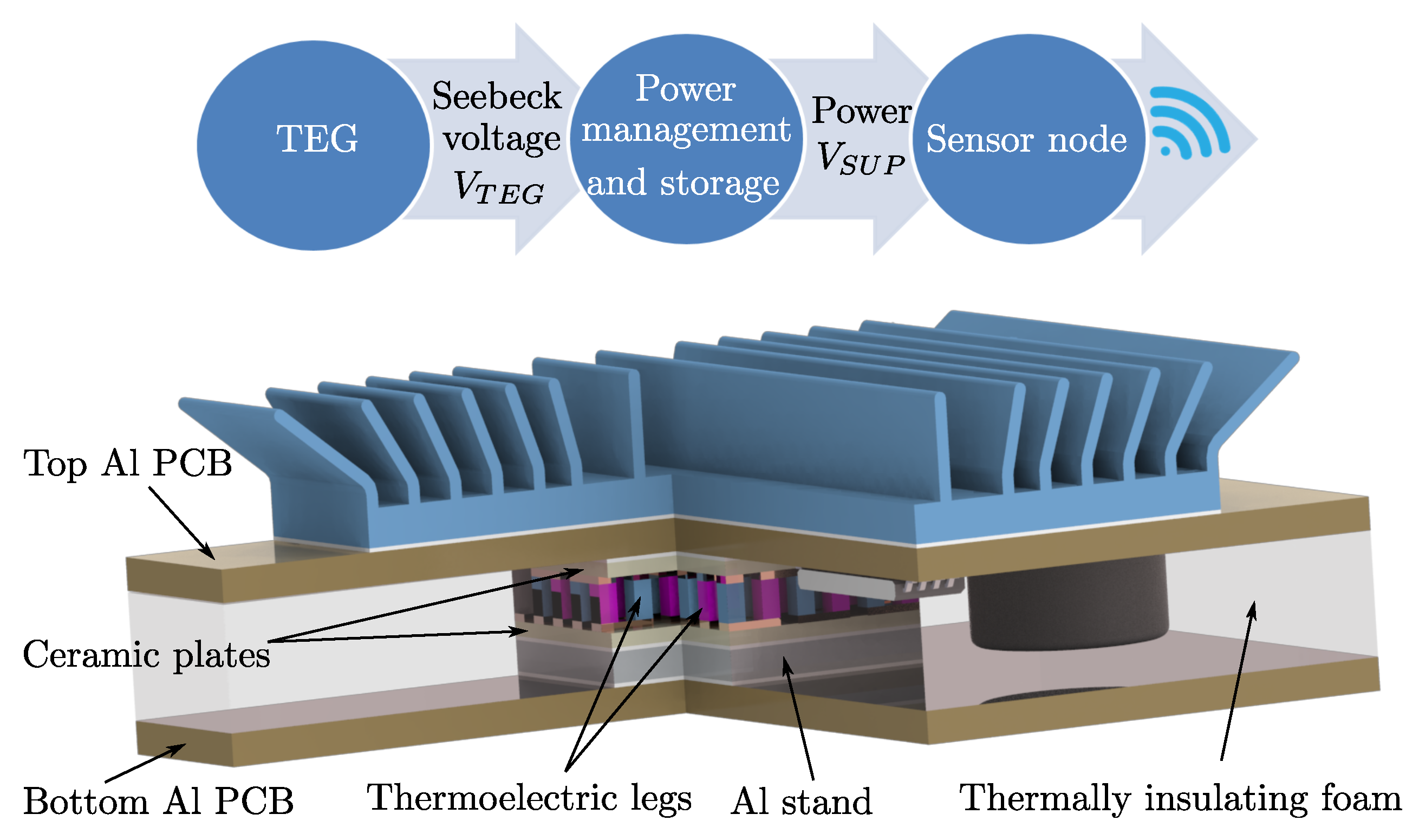
The investigated wireless sensor network node is realized as a stacked structure (Figure 1) confined by two aluminum core printed circuit boards (PCBs) with an aluminum heatsink mounted on the top PCB [9,39]. An aluminum stand is placed between the bottom PCB and TEG to compensate different heights of the used electronic devices. The bottom PCB is exposed to a heat source and it acts as a heat collector for the hot side of the TEG. The top PCB, in conjunction with the heatsink, is an additional heat spreader for the cold side of the TEG. Most of the electronic components are placed on the inner side of the top PCB, while the temperature sensor is on the inner side of the bottom PCB. Thermal glue is used to obtain a good mechanical and thermal connection between parts of the system. Thermally insulating foam fills space between the PCBs in order to reduce undesirable heat exchange. The main part of the system is a commercial thermoelectric module, based on Bi${}_2$Te${}_3$ alloy, which is used as a thermoelectric generator to provide power for the node. Tens degrees of the temperature difference between hot and cold side of the TEG enables the generation of the Seebeck voltage up to several hundreds of mV. This voltage value is not sufficient for the powering of electronic devices and it is introduced into the block for power management and storage, which enables a continuous supply of the WSN node (Figure 1). A step-up converter LTC3108 [40] with 1:100 ratio transformer at the input, two 220 μF tantalum capacitors as a primary storage and 0.2 F supercapacitor as a backup storage are exploited. The large backup capacitor is used to supply the WSN node when the heat source is not capable to generate voltage necessary for the functioning of the step-up circuitry. Other parts of the WSN node are a temperature sensor, microcontroller PIC16F684 for the acquisition of measured data and 434 MHz RF module for wireless data transmission. The main characteristics of the node are its compactness with overall dimensions of (52 × 35 × 17.6) $\mathrm{m}\mathrm{m}$, reliable cold booting and extended autonomy under unsuitable ambient thermal conditions [39].

3. SPICE Model of the TEG and WSN Node

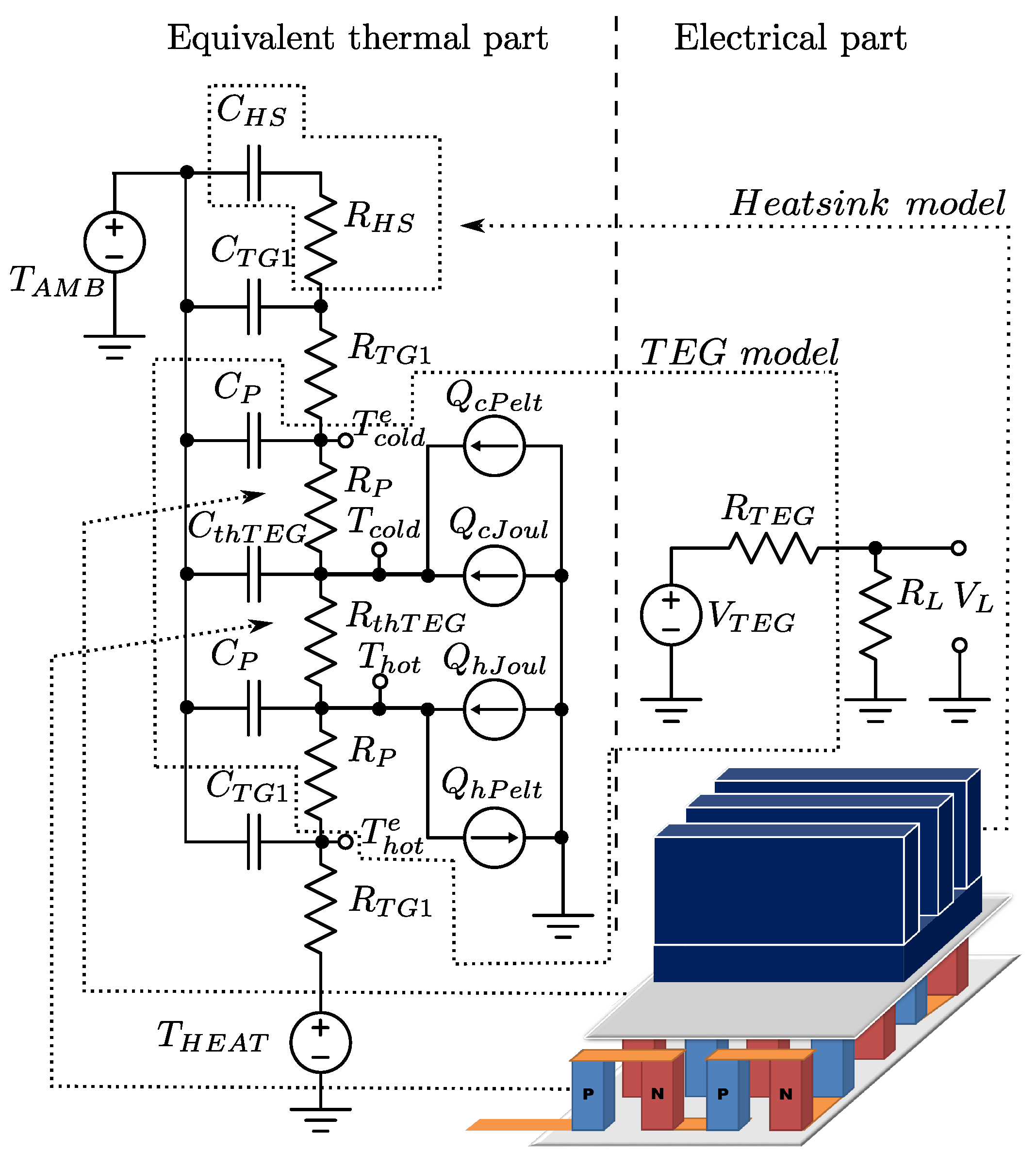
The TEG model should replicate as accurately as possible the real behavior of the device. This is important in order to evaluate which TEG is the best for a specified energy harvesting system. The equivalent SPICE electro-thermal model of the TEG with heatsink was realized with lumped parameter elements as presented in Figure 2.

The analogy between quantities characteristic for the electrical and thermal domains given in

Table 1. The analogy between electrical and thermal quantities [16].

Electrical Quantity	Thermal Quantity
Voltage $V\left(\mathrm{V}\right)$	Absolute temperature $T\left(\mathrm{K}\right)$
Current $I\left(\mathrm{A}\right)$	Heat rate $Q\left(\mathrm{W}\right)$
Resistance $R\left(\mathsf{\Omega }\right)$	Thermal resistance $R_{th}(\mathrm{K}\hspace{0.17em}{\mathrm{W}}^{-1})$
Capacitance $C\left(\mathrm{F}\right)$	Thermal capacitance $C_{th}(\mathrm{J}\hspace{0.17em}{\mathrm{K}}^{-1})$

is utilized for the model. Therefore, the network consists of the equivalent thermal part and the electrical part. The Cauer (T or ladder) network, which is a grounded-capacitor thermal network, is used to model heat transfer through the TEG. The main advantage of this network is that it is derived from the fundamental heat transfer physics [41] and allows access to the internal temperatures between the node parts. The equivalent electro-thermal model is developed with the assumption that dominant effects in the TEG are Seebeck, Peltier and Joule, while the Thompson effect is minor in the applicable temperature difference range and therefore neglectable [34,42]. Heat flow through the device is considered one-directional, while the Seebeck coefficient and electrical resistances are temperature-dependent parameters. Due to the copper high thermal conductivity and a small volume of connectors, their thermal resistances and capacitances are not included in the thermal part of the TEG model. The low electrical resistivity of copper justifies the absence of the connectors resistances in the electrical part of the model. Also, due to the small number of the thermoelectric pairs, the parasitic reactive electrical elements are not considered [21].

The Seebeck voltage will be generated when two sides of the TEG are at different temperatures:

$$V_{TEG}=N{\alpha }_{pn}(T_{hot}-T_{cold}),$$

(1)

where N is the number of thermoelectric pairs, ${\alpha }_{pn}={\alpha }_p-{\alpha }_n$ is value of the overall Seebeck coefficient, $T_{hot}$ and $T_{cold}$ are temperatures at the hot and cold sides of the TEG legs, respectively. The Seebeck coefficient is a temperature dependent parameter with the value ${\alpha }_{pn0}$ at a reference temperature $T_0=298\hspace{0.17em}\mathrm{K}$ and temperature coefficient $a_{\alpha }$. In the simulations, its value is calculated for the mean temperature in the TEG, $(T_{hot}+T_{cold})/2$. Therefore, thermally generated voltage is modeled in SPICE by the voltage controlled voltage source ($V_{TEG}$):

$$V_{TEG}=N{\alpha }_{pn0}\left[1+a_{\alpha }\left(\frac{T_{hot}+T_{cold}}{2}-T_0\right)\right](T_{hot}-T_{cold}).$$

(2)

The electrical resistance of all TEG legs is its internal resistance:

$$R_{TEG0}=\frac{2N{\rho }_{0}l}{A},$$

(3)

where ${\rho }_0={\rho }_n={\rho }_p$ is the electrical resistivity of thermoelectric materials at the reference temperature $T_0$, l is the length and A is the cross-sectional area of an individual leg. In SPICE model, $R_{TEG}$ is also considered as temperature dependent:

$$R_{TEG}=R_{TEG0}\left[1+a_{\rho }\left(\frac{T_{hot}+T_{cold}}{2}-T_0\right)\right],$$

(4)

where $a_{\rho }$ is temperature coefficient of electrical resistivity. By connecting load $R_L$ to the TEG, an electrical circuit is formed, enabling a flow of electrical current (Figure 2):

$$I_L=I_{TEG}=\frac{V_{TEG}}{R_{TEG}+R_L}.$$

(5)

The Peltier effect appears in the presence of an electrical current and depends on the absolute temperature and overall Seebeck coefficient. It causes heat absorption of the rate $Q_{cPelt}$ at the cold side and heat dissipation of the rate $Q_{hPelt}$ at the hot side of the pairs:

$$Q_{cPelt}=N{\alpha }_{pn0}\left[1+a_{\alpha }\left(\frac{T_{hot}+T_{cold}}{2}-T_0\right)\right]T_{cold}{I}_{TEG},$$

(6)

$$Q_{hPelt}=N{\alpha }_{pn0}\left[1+a_{\alpha }\left(\frac{T_{hot}+T_{cold}}{2}-T_0\right)\right]T_{hot}{I}_{TEG}.$$

(7)

The operation of the TEG is also governed by the Joule effect. It manifests as a heat dissipated by material with non-zero resistance in the presence of an electrical current ($Q_{Joul}$) which is evenly absorbed by hot ($Q_{hJoul}$) and cold ($Q_{cJoul}$) sides:

$$Q_{cJoul}=Q_{hJoul}=\frac{1}{2}{Q}_{Joul}=\frac{1}{2}{V}_{RTEG}{I}_{TEG},$$

(8)

where $V_{RTEG}=V_{TEG}-V_L=I_{TEG}{R}_{TEG}$. The Peltier heat rates defined by (6) and (7), as well as the Joule effect given by (8), are modeled with the arbitrary behavioral current generators $Q_{cPelt}$, $Q_{hPelt}$, $Q_{cJoul}$ and $Q_{hJoul}$.

Heat conduction through the TEG legs from the hot to the cold side is described by Fourier law:

$$Q_{cond}=\frac{T_{hot}-T_{cold}}{R_{thTEG}}.$$

(9)

Here $R_{thTEG}$ represents the thermal resistance of all TEG legs and it is given by:

$$R_{thTEG}=\frac{l}{2N\lambda A},$$

(10)

where $\lambda ={\lambda }_n={\lambda }_p$ is the thermal conductivity of thermoelectric materials. Overall heat rates absorbed at the hot side of TEG legs ($Q_h$) and released to the environment at the cold side ($Q_c$) are balanced according to the relations:

$$Q_h=Q_{hPelt}+Q_{cond}-Q_{hJoul},$$

(11)

$$Q_c=Q_{cPelt}+Q_{cond}+Q_{cJoul}.$$

(12)

These heats flow through the ceramic plates of the TEG toward its external sides at temperatures $T_{hot}^e$ and $T_{cold}^e$, according to the Fourier law:

$$Q_h=\frac{T_{hot}^e-T_{hot}}{R_P},$$

(13)

$$Q_c=\frac{T_{cold}-T_{cold}^e}{R_P}.$$

(14)

The ceramic plate thermal resistance ($R_P$) is given by:

$$R_P=\frac{l_P}{{\lambda }_P{A}_{TEG}},$$

(15)

where $l_P$ is the thickness of the ceramic plate, ${\lambda }_P$ is ceramics thermal conductivity and $A_{TEG}$ is the external TEG area. Additional elements in Figure 2 are thermal resistances and capacitances of the heatsink ($R_{HS}$, $C_{HS}$) and thermal glue ($R_{TG1}$, $C_{TG1}$). Voltage generators $T_{HEAT}$ and $T_{AMB}$ are equivalents of the heat source and ambient temperature, respectively.

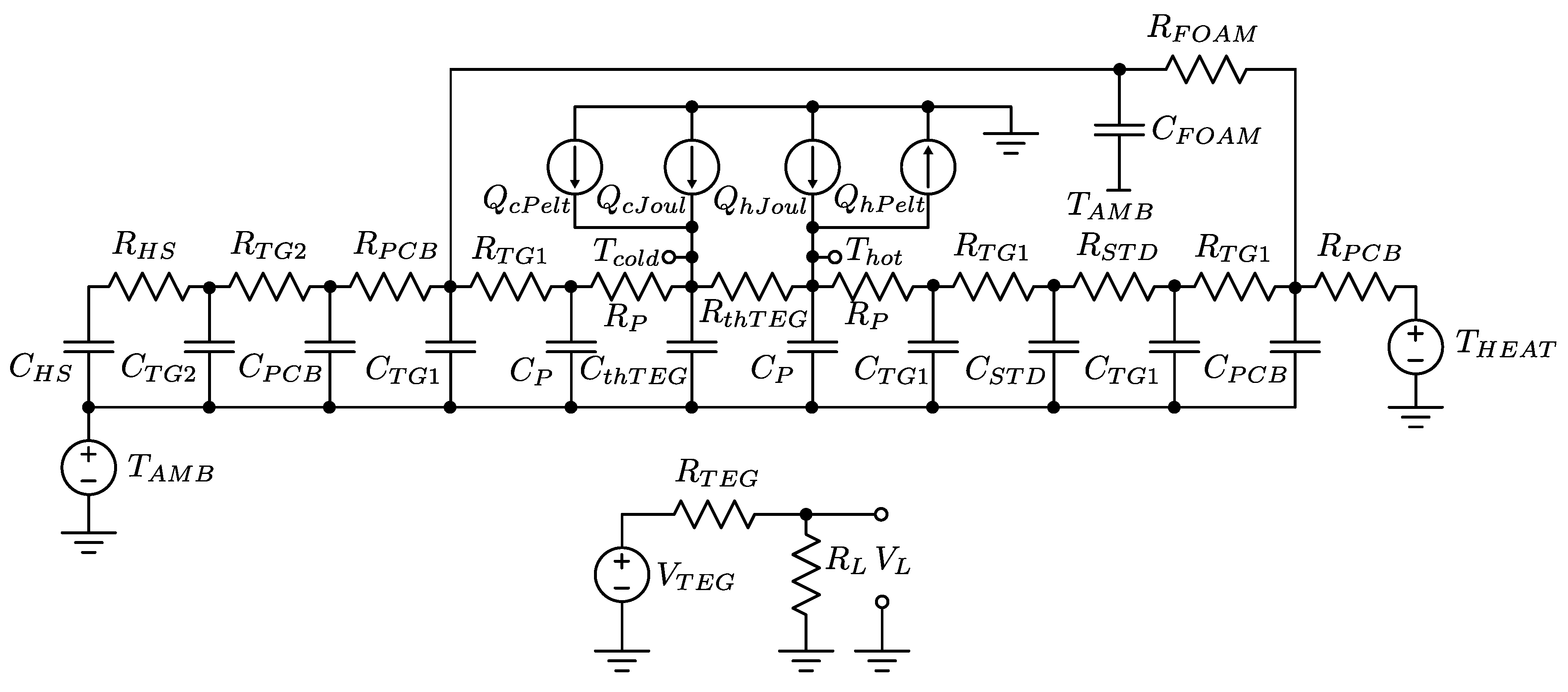
The model of the WSN node is built on the basis of the electro-thermal model of the TEG. All constitutive elements introduce thermal resistances and capacitances connected at the appropriate nodes of the network. SPICE model schematic of the WSN node is shown in Figure 3. Thermal resistances of the PCB, thermal glue and aluminum stand, given in

Table 2. Thermal resistances of the WSN node elements.

WSN Node Element →	Aluminum PCB	Thermal Glue TG1/TG2	Thermal Foam	Aluminum Stand
Parameter
Thermal conductivity ${\lambda }_x$ (W m−1 K−1)	153	1.1	0.4	153
Thickness $l_x$ ($\mathrm{m}\mathrm{m}$)	1.7	0.2	6.5	1.6
Cross-sectional area $A_x$ (${\mathrm{m}\mathrm{m}}^2$)	1820	225/1225	1595	225
Thermal resistance $R_{thx}$ (K W−1)	0.0061	0.81/0.148	10.18	0.0465

, are determined by their length (thickness) ($l_x$), cross-sectional area ($A_x$) and thermal conductivity of their materials (${\lambda }_x$) by:

$$R_{thx}=\frac{l_x}{{\lambda }_x{A}_x}.$$

(16)

The thermal resistance of the insulating foam is modeled by a high-value resistor in a feedback loop of the electrical network. This thermal resistance is given as:

$$R_{FOAM}=\frac{l_{foam}}{{\lambda }_{foam}(A_{PCB}-A_{TEG})}.$$

(17)

The values of the heatsinks thermal resistances are taken from their datasheets.

Thermal capacitance is a measurable physical quantity equal to the ratio of the heat added to/removed from an object and the resulting temperature change. Accordingly, the specific heat capacity of a material in the absence of phase transitions on a per mass basis is equivalent to:

$$c=\frac{C_{th}}{m}=\frac{C_{th}}{dV},$$

(18)

where $C_{th}$ is the thermal capacitance of an object made of the specific material, d is the density of the object material, m is the mass of the object and V is its volume. Therefore, the values of the thermal capacitances for WSN node elements given in

Table 3. Thermal capacitances of the WSN node elements.

WSN Node Element →	Aluminum PCB	Thermal Glue TG1/TG2	Thermal Foam
Parameter
Specific heat capacit $c_x$ ($\mathrm{J}\hspace{0.17em}{\mathrm{g}}^{-1}\hspace{0.17em}{\mathrm{K}}^{-1}$)	0.92	2.09	0.82
Density $d_x$ ($\mathrm{g}\hspace{0.17em}{\mathrm{c}\mathrm{m}}^{-3}$)	2.7	2.44	0.58
Volume $V_x$(${\mathrm{c}\mathrm{m}}^3$)	3.09	0.045/0.245	23.13
Thermal capacitance $C_{thx}$ ($\mathrm{J}\hspace{0.17em}{\mathrm{K}}^{-1}$)	7.685	0.229/1.251	11

are calculated as:

$$C_{thx}=c_x{d}_x{V}_x.$$

(19)

The electrical load of the node ($R_L$) is defined by the input resistance of the step–up converter LTC3108 when it charges primary and backup capacitors. It is simulated by a behavioral resistor whose resistance changes with the current flowing through it. The $R_L$ resistance values for the different $I_L$ current values shown in

Table 4. Dependence of the WSN node load resistance on the load current [40].

$I_L$ ($\mathrm{m}\mathrm{A}$)	0	3	5	7.3	9	10	13	20	26	30	79	100	200
$R_L$ ($\mathsf{\Omega })$	10	7	5	4.1	4	3.9	3.8	3	2.7	2.7	2.5	2.5	2.5

were determined from the datasheet of LTC3108 [40]. The appropriate values are set through the lookup table with linear interpolation. This approach is chosen due to the simple implementation into the circuit simulator with acceptable accuracy [9,13].

4. Experimental Setup

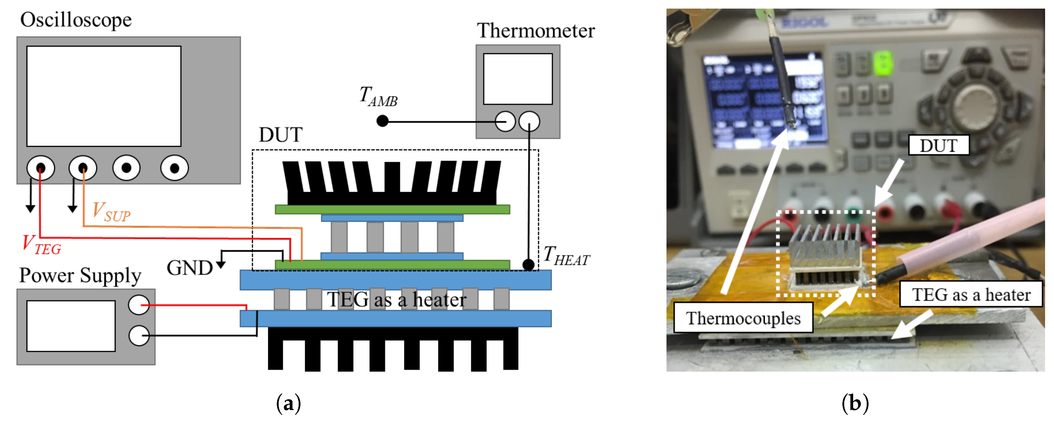
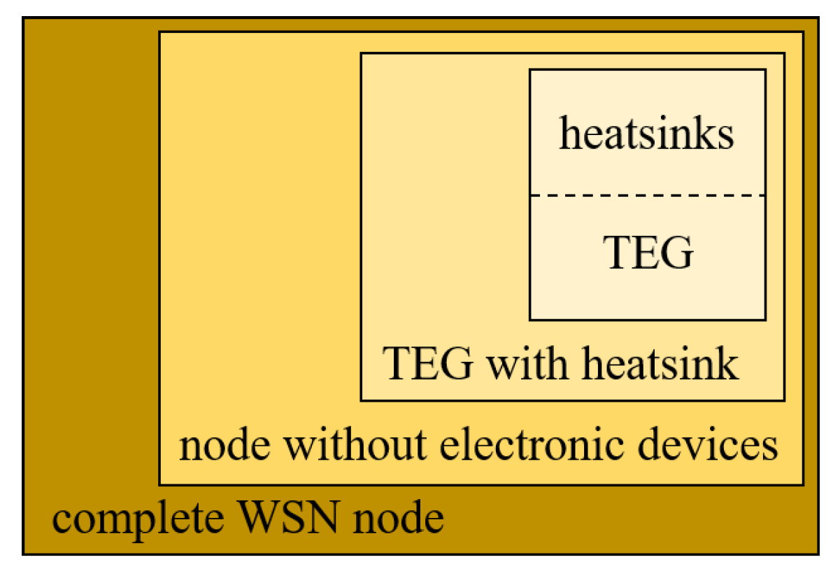
Block diagram and photograph of the experimental setup are shown in Figure 4a,b, respectively. This setup enables controlled input of the heat flux and measurement of the relevant temperatures and voltages in the time domain. A device under test (DUT) was placed onto the heater horizontally, as the worst-case design for the heat dissipation process. Constant heat flux to the hot side of the DUT is obtained by the appropriate thermoelectric (Peltier) module. This heater is supplied by the current of 0.5–2 A from laboratory programmable DC power supply while a large aluminum heatsink is used to remove heat from its cold side. In the experiments, different DUTs were: two heatsinks; standalone TEG; TEG in conjunction with a heatsink; WSN node with and without accompanying electronics. The thermal glue is used to provide good thermal contact between the heater and investigated DUT. The thermometer with 2 thermocouples was used to measure the temperature of ambient ($T_{AMB}$) and the relevant temperature of the specific DUT. Those are heatsink fins temperature ($T_{HS}$), TEG cold side temperature ($T_{cold}$) and WSN node hot side temperature ($T_{hot}$) or temperature of the heater ($T_{HEAT}$). The voltage generated by the TEG ($V_{TEG}$) and power supply voltage of the WSN node ($V_{SUP}$) were acquired by an oscilloscope.

For this study, the thermoelectric module ET-031-10-20 by Adaptive (denoted as TEG1) and two low profile aluminum heatsinks were selected. The heatsink A, with ribbed geometry and dimensions (15 × 15 × 5) $\mathrm{m}\mathrm{m}$, has the base surface equal to the TEG1 area while the flared fin heatsink B of dimensions (35 × 35 × 7.5) $\mathrm{m}\mathrm{m}$ is part of the investigated WSN node described in Section 2.

5. Results and Discussion

The model is verified by LTSpice [43] simulations of the WSN node gradually. The block diagram in Figure 5 shows the model verification steps. Firstly, the basic TEG model was validated, and afterward, the model was upgraded with elements describing the heatsink. Subsequently, parts of the WSN node without electronic devices were taken into account through appropriate thermal resistances and capacitances, and finally, the complete WSN node model was verified.

As the main part of the WSN node, three different TEGs from two manufacturers were considered in simulations. Selected TEGs have internal electrical resistances close to the impedance matched conditions ($R_{TEG}=R_L$), to enable operation around the maximum power transfer from the generator (TEG) to the load (LTC3108 circuit). TEGs differ in the thermoelectric pairs number, material parameters, and dimensions of the thermoelectric legs and ceramic plates. Values of the characteristic geometrical, electrical and thermal parameters of the considered TEGs, as well as values of the equivalent network elements calculated using (10), (15) and (19), are given in

Table 5. Properties of the considered TEGs.

Manufacturer Part No. →	ET–031-10-20 (TEG1)	MCPE–071-10-15 (TEG2)	CP–08,31,06 (TEG3)
Parameter
Maximum operating temperature $T_{max}$ ($°\mathrm{C}$) *	90	110	80
Maximum temperature difference $\Delta T_{TEGmax}$ ($°\mathrm{C}$) *	75	72	67
Number of thermoelectric pairs N *	31	71	31
External dimensions L × W × H ($\mathrm{m}\mathrm{m}$) *	15 × 15 × 4.3	20 × 20 × 3.8	12 × 12 × 3.3
Area of the TEG $A_{TEG}$ (mm2)	225	400	144
Thermoelectric leg dimensions w × w × l ($\mathrm{m}\mathrm{m}$) *	1 × 1 × 2	1 × 1 × 1.5	0.8 × 0.8 × 1.5
Ceramic plate thickness $l_P$ ($\mathrm{m}\mathrm{m}$)	0.75	0.75	0.6
Overall Seebeck coefficient ${\alpha }_{pn0}$ ($\mathsf{\mu }\mathrm{V}\hspace{0.17em}{\mathrm{K}}^{-1}$)	396	396	378
Temperature coefficient of ${\alpha }_{pn}$ − $a_{\alpha }$ (${\mathrm{K}}^{-1}$)	$2·{10}^{-3}$
Thermoelectric leg thermal conductivity $\lambda$ ($\mathrm{W}\hspace{0.17em}{\mathrm{m}}^{-1}\hspace{0.17em}{\mathrm{K}}^{-1}$)	1.5	1.5	1.7
Ceramic plate thermal conductivity ${\lambda }_P$ ($\mathrm{W}\hspace{0.17em}{\mathrm{m}}^{-1}\hspace{0.17em}{\mathrm{K}}^{-1}$)	25
Electrical resistivity of the thermoelectric leg ${\rho }_0$ ($\mathsf{\mu }\mathsf{\Omega }\hspace{0.17em}\mathrm{m}$)	11.4	11.4	10.6
Temperature coefficient of $\rho$ − $a_{\rho }$ (${\mathrm{K}}^{-1}$)	$3.4·{10}^{-3}$
Ceramic plate thermal resistance $R_P$ ($\mathrm{K}\hspace{0.17em}{\mathrm{W}}^{-1}$)	0.13	0.075	0.16
Internal thermal resistance $R_{thTEG}$ ($\mathrm{K}\hspace{0.17em}{\mathrm{W}}^{-1}$)	21.74	7.04	22.22
Internal electrical resistance $R_{TEG0}$ ($\mathsf{\Omega }$)	1.41	2.43	1.54
Thermoelectric leg density $d_{TEG}$ ($\mathrm{g}\hspace{0.17em}{\mathrm{c}\mathrm{m}}^{-3}$)	7.74
Ceramic plate density $d_P$ ($\mathrm{g}\hspace{0.17em}{\mathrm{c}\mathrm{m}}^{-3}$)	3.57
Thermoelectric leg specific heat capacity $c_{TEG}$ ($\mathrm{J}\hspace{0.17em}{\mathrm{g}}^{-1}\hspace{0.17em}{\mathrm{K}}^{-1}$)	0.165
Ceramic plate specific heat capacity $c_P$ ($\mathrm{J}\hspace{0.17em}{\mathrm{g}}^{-1}\hspace{0.17em}{\mathrm{K}}^{-1}$)	0.837
Thermoelectric legs volume $V_{TEG}$ (${\mathrm{c}\mathrm{m}}^3$)	0.124	0.213	0.059
Ceramic plate volume $V_P$ (${\mathrm{c}\mathrm{m}}^3$)	0.169	0.3	0.086
Thermal capacitance of thermoelectric legs $C_{thTEG}$ ($\mathrm{J}\hspace{0.17em}{\mathrm{K}}^{-1}$)	0.158	0.272	0.075
Thermal capacitance of ceramic plate $C_P$ ($\mathrm{J}\hspace{0.17em}{\mathrm{K}}^{-1}$)	0.504	0.896	0.258

* Parameter taken from datasheet.

.

A practical method for handling transient thermal problems is to measure the thermal response of an object to a step input thermal power. Using the electro-thermal analogy for the RC circuit, variation of the object temperature in time after instantaneously applied temperature difference at its base can be expressed as:

$$\Delta T\left(t\right)=\Delta T_0\left(1-e^{-{\displaystyle \frac{t}{{\tau }_{th}}}}\right),$$

(20)

where $\Delta T_0$ is the maximum change in the temperature of the object (steady–state when its thermal capacitance is fully charged) and ${\tau }_{th}=R_{th}{C}_{th}$ is the thermal time constant of the object.

Therefore, if the heatsink is described with a grounded thermal model, it is necessary to determine its thermal resistance and thermal capacitance. The values of thermal resistances in stagnant air of the heatsinks A and B, based on their datasheets, are $R_{thA}=12\hspace{0.17em}\mathrm{K}\hspace{0.17em}{\mathrm{W}}^{-1}$ and $R_{thB}=11\hspace{0.17em}\mathrm{K}\hspace{0.17em}{\mathrm{W}}^{-1}$. Time dependences of the heatsinks fins temperatures $T_{HS}$ relative to $T_{AMB}$ when temperature difference of $\Delta T=T_{HEAT}-T_{AMB}=20\hspace{0.17em}°\mathrm{C}$ is applied at their bases are shown in Figure 6. These dependencies follow (20) and values of $\Delta T_0$ and ${\tau }_{th}$ can be determined numerically. The obtained values are $\Delta T_{0A}=13.6\hspace{0.17em}°\mathrm{C}$, ${\tau }_{thA}=22.47\hspace{0.17em}\mathrm{s}$, $\Delta T_{0B}=11.22\hspace{0.17em}°\mathrm{C}$, ${\tau }_{thB}=27.93\hspace{0.17em}\mathrm{s}$, which for thermal capacitances gives $C_{thA}=C_{HSA}=1.88\hspace{0.17em}\mathrm{J}\hspace{0.17em}{\mathrm{K}}^{-1}$ and $C_{thB}=C_{HSB}=2.54\hspace{0.17em}\mathrm{J}\hspace{0.17em}{\mathrm{K}}^{-1}$.

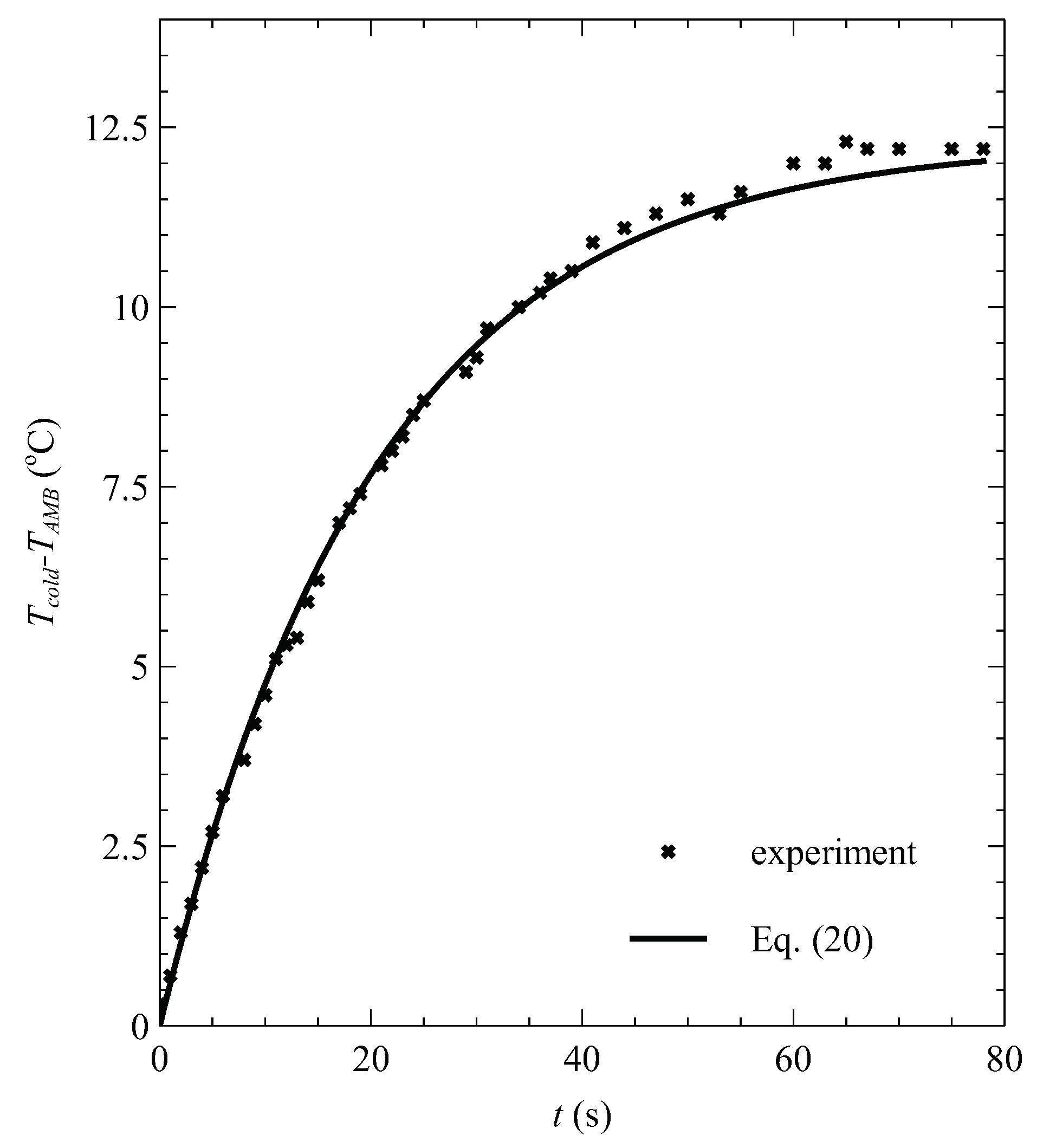
The TEG is modeled by three pairs of thermal resistances and capacitances which correspond to the thermoelectric legs and two ceramic plates. If the equivalent thermal resistance is presented as the sum of corresponding quantities for each part of the TEG1 (see Figure 2), it is obtained: $R_{e-thTEG}=R_P+R_{thTEG}+R_P\simeq R_{thTEG}=22\hspace{0.17em}\mathrm{K}\hspace{0.17em}{\mathrm{W}}^{-1}$. The equivalent thermal capacitance is calculated as: $C_{e-thTEG}=C_P+C_{thTEG}+C_P=1.17\hspace{0.17em}\mathrm{J}\hspace{0.17em}{\mathrm{K}}^{-1}$. These analytically obtained results were experimentally confirmed by measurement of the TEG1 cold side temperature $T_{cold}$ relative to the ambient temperature as a response to the applied temperature difference $\Delta T=T_{HEAT}-T_{AMB}=15\hspace{0.17em}°\mathrm{C}$ as shown in Figure 7. Numerically extracted value of the thermal time constant is ${\tau }_{e-thTEG}=25.66\hspace{0.17em}\mathrm{s}$, while for thermal capacitance is calculated $C_{e-thTEG}=1.19\hspace{0.17em}\mathrm{J}\hspace{0.17em}{\mathrm{K}}^{-1}$ which is close to the analytically obtained value ( $1.17$ $\mathrm{J}\hspace{0.17em}{\mathrm{K}}^{-1}$.

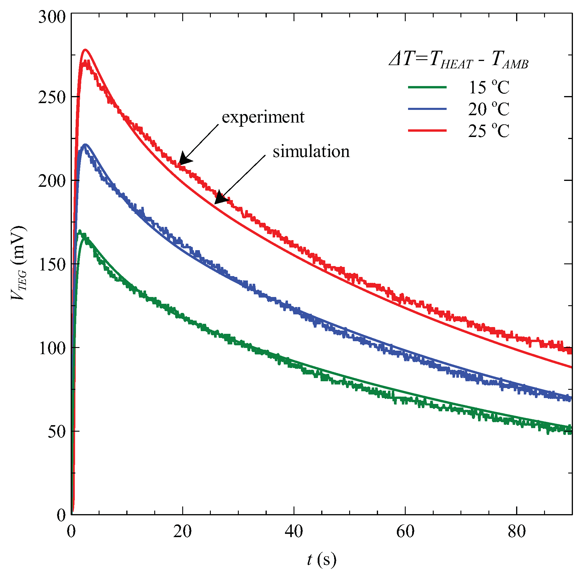
To verify the SPICE model of the TEG1 with heatsink, additional thermal response characterization was performed. The aluminum ribbed heatsink A was glued on the TEG1 cold side while its hot side was placed onto the heated surface of the constant temperature. The generated voltage was recorded by the oscilloscope and compared with the values obtained by LTSpice simulations (circuit in Figure 2). The electrical load of the network was defined as a very large ( 10 $\mathrm{M}$$\mathsf{\Omega }$), so $V_L=V_{TEG}$. The experiments and simulations were performed for three temperature differences as shown in Figure 8.

Firstly, generated voltage increases abruptly due to the applied thermal input at the TEG hot side and after reaching the peak value, it decreases gradually with time. The decrease follows the temperature response of the heatsink as its thermal capacitance charges through the TEG. It reaches the equilibrium state when the heatsink is unable to sink excess heat, i.e. when its thermal capacitance is fully charged. The peak values of the generated voltage are from 170 $\mathrm{m}$$\mathrm{V}$ at $\Delta T=15\hspace{0.17em}°\mathrm{C}$ up to 278 $\mathrm{m}$$\mathrm{V}$ at $\Delta T=25\hspace{0.17em}°\mathrm{C}$. It can be seen that excellent agreement between experimental and simulation results is achieved. The maximum deviation between the results is 4.12%. This verifies the applicability of the presented model for the characterization of different TEGs as part of the considered WSN node.

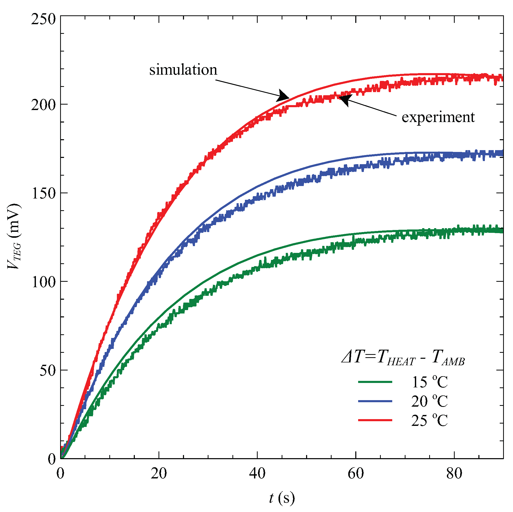
The thermal response of the whole node structure with TEG1 is presented in Figure 9 by the dependence of the generated voltage in time. All constitutive elements except the electronic devices are included. Exchange of the heat between the node and ambient is obtained by the aluminum heatsink B. Three temperature differences between the hot side of the node and the ambient have been explored, with $\Delta T=15\hspace{0.17em}°\mathrm{C}$ as the minimum designed value [39]. Again, the load resistance is high and $V_L=V_{TEG}$. The load voltage increases slowly and reaches a constant value after several tens of seconds. After 90 $\mathrm{s}$, its value is from 130 $\mathrm{m}$$\mathrm{V}$ at $\Delta T=15\hspace{0.17em}°\mathrm{C}$ up to 215 $\mathrm{m}$$\mathrm{V}$ at $\Delta T=25\hspace{0.17em}°\mathrm{C}$. The response of the system is governed by the thermal coupling between the TEG, heatsink and other WSN node building elements characterized by the time needed for their thermal capacitances to be charged. In this case, the heat is transferred from the heater to the bottom PCB and afterward to the rest of the system mainly through the aluminum stand and TEG. Heat transfer through the thermal foam is minimal since it has a considerably larger thermal resistance. The top PCB has an important role in the heat release since it acts as an extension of the heatsink base. Due to the coupled thermal processes, the voltage overshoot can be slightly noticed only at higher $\Delta T$ and after a longer period than for the TEG-heatsink assembly. The values of the TEG voltage determined by the simulation, with this set of model parameters, match well the experimentally obtained values. The maximum deviation between the results is 6.25% and it can be explained by simplified simulation conditions. For example, it is not possible to predict fluctuations in the air temperature that can influence the experimental results.

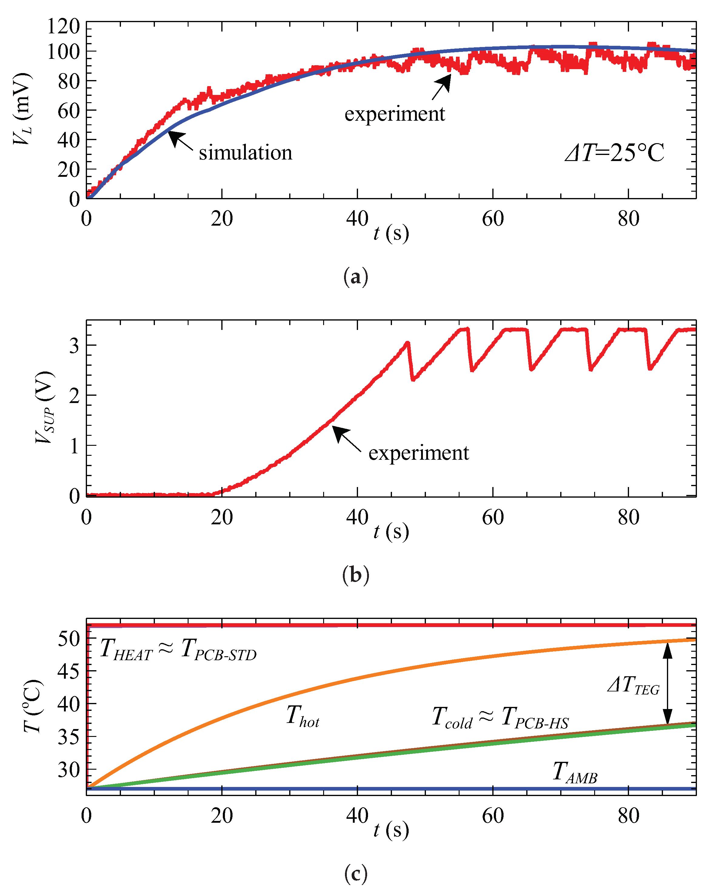
An in-depth analysis of the complete WSN node was made by monitoring load voltage for the temperature difference $\Delta T=T_{HEAT}-T_{AMB}$ of 25 $°\mathrm{C}$. The results of the experiment and simulations are shown in Figure 10a.

Dependences of the generated voltage for the WSN node without electronic devices (Figure 9) and load voltage for the complete node are similar, but in the second case voltage values are 50% lower due to the presence of the load resistance and the Peltier effect ($V_L\ne V_{TEG}$). Furthermore, by adding electronic components, the thermal foam volume in the WSN node decreases and therefore its thermal capacitance also decreases. Experimentally measured voltages have the drops at time instances when the WSN node transmits data and draws substantial current from the charge reservoirs connected to the step-up converter. Due to the internal configuration and operation principle of the converter LTC3108 these ocilations are reflected to its input i.e. to the load voltage. The simulation results match very well the average value of the load voltage in the interval of full operation.

In Figure 10b, the experimental values of the WSN node power supply voltage obtained by the step-up converter ($V_{SUP}$) are given. Comparing this figure with Figure 10a, it is evident that start–up of the LTC3108 circuit and charging of the primary storage capacitors begin when the load voltage is about 60 $\mathrm{m}$$\mathrm{V}$, which requires 17 $\mathrm{s}$. After additional 30 $\mathrm{s}$, the supply voltage reaches a value of 3 $\mathrm{V}$, sufficient for the start–up of the microcontroller and the overall cold boot time is 47 $\mathrm{s}$. The microcontroller discharges the primary capacitors to some extent while the existing temperature difference enables their subsequent recharge to $3.3$ $\mathrm{V}$. This discharge-recharge process, similarly as in the case of the load voltage, occurs each time the microcontroller acquires and sends data (every 8 $\mathrm{s}$).

The advantage of the Cauer type network, used in the presented SPICE model, is access to the internal network nodes’ temperatures. Accordingly, the temperature distribution within the WSN node obtained by simulation is presented in Figure 10c. It can be seen that, after positioning the node onto the heater, the heat is almost instantly transferred through the bottom PCB to the aluminum stand and then gradually to the TEG. After 90 $\mathrm{s}$ (approaching the system steady–state), the temperature difference between the heater and the hot side of the TEG is $2\hspace{0.17em}°\mathrm{C}$. At the same time, TEG heats up and the temperature at its interface with the top PCB increases. The temperature at the top PCB-heatsink interface is negligibly smaller than the temperature at TEG-top PCB interface. The effective temperature difference between the hot and cold side of the TEG is $\Delta T_{TEG}=13\hspace{0.17em}°\mathrm{C}$, while the temperature difference between the base of the heatsink which is glued to the top PCB and the ambient is $10\hspace{0.17em}°\mathrm{C}$. These results are in agreement with the data obtained by the thermovision imaging considered in [39].

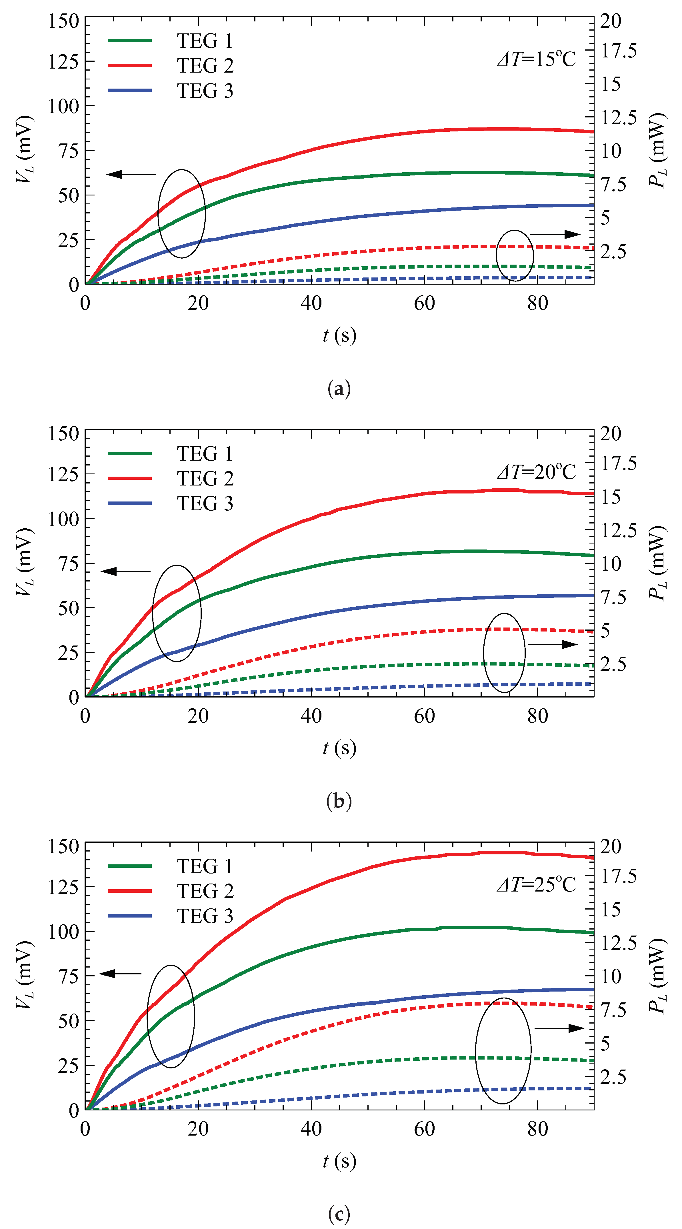
The proposed model is used for the characterization of three TEGs from Table 5 as parts of the considered WSN node structure. Overall dimensions of the node are adjusted to the implemented TEG by appropriate sizing of the aluminum PCBs, stand and thermal foam. Dependencies of the load voltage ($V_L$) and load power ($P_L$) at three temperature differences are presented in Figure 11.

As expected, an increase in the temperature difference increases the load voltage and power. TEG2 produces the highest values, and this advantage is more pronounced for greater $\Delta T$. After 90 $\mathrm{s}$, at a temperature difference of 25 $°\mathrm{C}$, the load voltage for TEG2 is 140 $\mathrm{m}$$\mathrm{V}$ which is 40% larger than 100 $\mathrm{m}$$\mathrm{V}$ for TEG1 and doubled in comparison to 70 $\mathrm{m}$$\mathrm{V}$ for TEG3. Also, the load power is from $1.6$ $\mathrm{m}$$\mathrm{W}$ for TEG3 up to $7.6$ $\mathrm{m}$$\mathrm{W}$ for TEG2. The overall system harvesting efficiency calculated as the ratio $P_L/Q_{HEAT}$ increases with the increase of the temperature difference. It rises from 0.04% for TEG3 at $\Delta T_{TEG}=15\hspace{0.17em}°\mathrm{C}$ over 0.11% for TEG1 at $\Delta T_{TEG}=20\hspace{0.17em}°\mathrm{C}$ toward 0.15% for TEG2 at $\Delta T_{TEG}=25\hspace{0.17em}°\mathrm{C}$. Low overall efficiency is a consequence of two main factors. The first is the low conversion efficiency of the TEGs at the small temperature gradients (1%–2%). The second is established temperature distribution through the node elements governed by the natural convection as the worst-case design for the heat dissipation mechanism. In general, the node with TEG2 would perform 20% better than TEG1 and 90% better than TEG3 for the same temperature difference. Better harvesting performances are a consequence of more than twice larger number of thermoelectric pairs in TEG2 (71) in comparison to TEG1 and TEG3 (31), and its internal electrical resistance which is closer to the impedance matched condition. However, due to the larger area, TEG2 implies a WSN node of 20% greater overall dimensions while for TEG3 its dimensions can be reduced for 15%. Although TEG1 and TEG3 have the same number of thermoelectric pairs and similar electrical and thermal resistances, TEG1 obtains about 50% higher load voltages due to the longer thermoelectric legs. Inside the WSN node, this property provides a higher temperature difference at the TEG sides which directly affects the value of the generated voltage and transferred power.

Results from Figure 11 are utilized for the estimation of the time necessary for start up of the power management circuit and subsequently the cold boot time of the WSN node. As commented for Figure 10b, load voltage of 60 $\mathrm{m}$$\mathrm{V}$ enables starting of the LTC3108. The temperature difference of $\Delta T=15\hspace{0.17em}°\mathrm{C}$ is insuficient for TEG3 to produce this voltage value, while for TEG1 and TEG2 it requires 47 $\mathrm{s}$ and 25 $\mathrm{s}$, respectively (Figure 11a). At $\Delta T=25\hspace{0.17em}°\mathrm{C}$ this voltage value is reached after 12 $\mathrm{s}$ for TEG2 up to 49 $\mathrm{s}$ for TEG3 (Figure 11c). Corresponding cold boot times determined from the load voltage dependencies are given in

Table 6. Cold boot times of WSN nodes with considered TEGs for different $\Delta T$.

$\Delta \mathit{T}$ ($°\mathbf{C}$)	TEG1	TEG2	TEG3
15	66 s	55 s	-
20	54 s	45 s	78 s
25	47 s	40 s	70 s

.

Better harvesting efficiency of TEG2 provides almost two times faster cold boot than TEG3 at $\Delta T=25\hspace{0.17em}°\mathrm{C}$. It is noticeable that TEG1 at specific temperature difference is as efficient as TEG2 for 5 $°\mathrm{C}$ lower $\Delta T$. Even though TEG3 demands higher temperature differences, it can be applied in cases where node dimensions represent a crucial design goal. It should be emphasized that, by performing simulations for the set of $\Delta T=T_{HEAT}-T_{AMB}$, the temperature difference necessary for the specific TEG to obtain predefined WSN node cold boot time can be determined in an efficient and simple way.

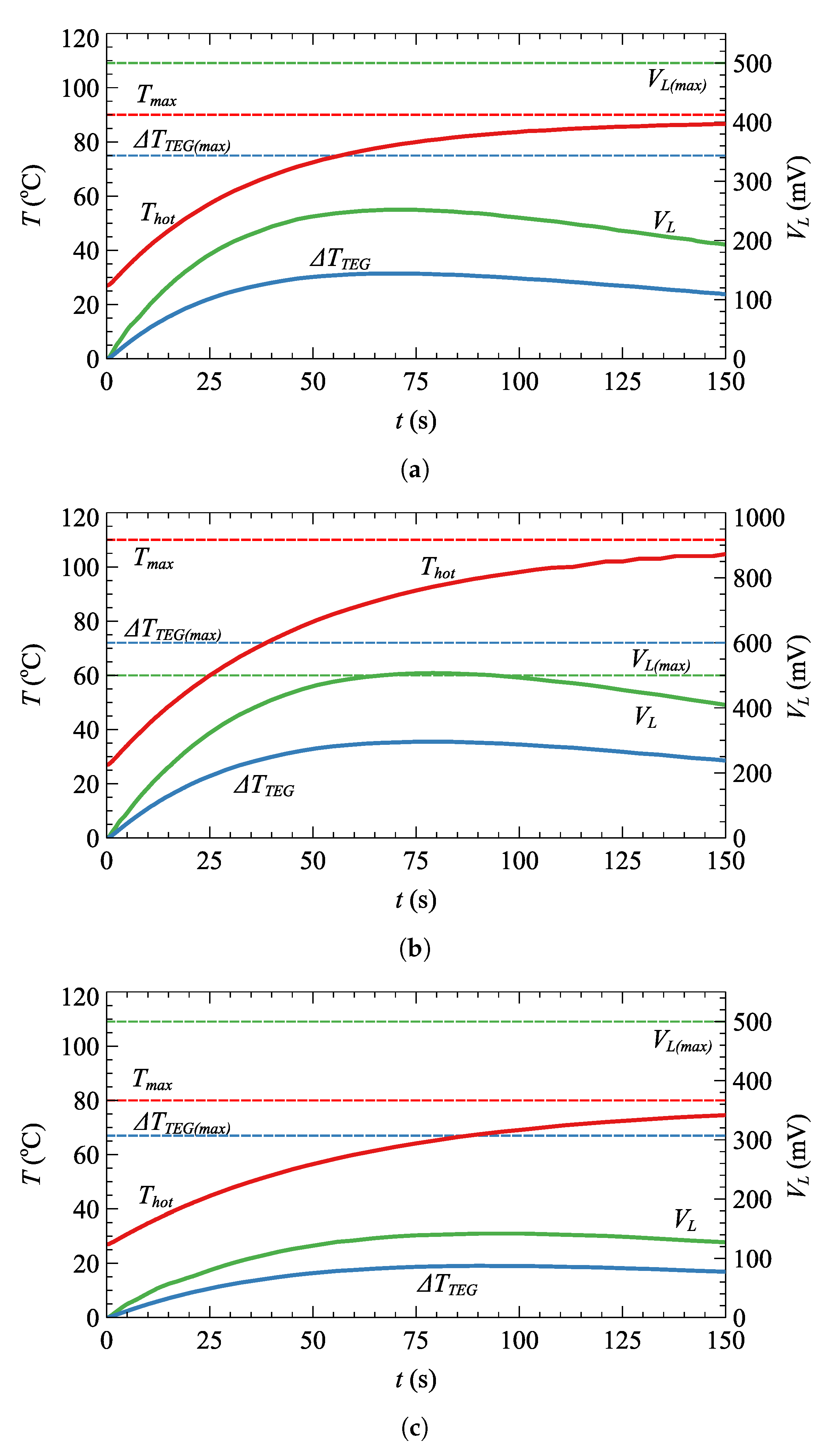
Data on temperature distributions inside the node (Figure 10c), enable to determine time dependencies of the hot ($T_{hot}$) and cold ($T_{cold}$) side temperatures, and the effective temperature difference at the TEG ($\Delta T_{TEG}$), when it is operated on the upper-temperature limit, as given in Figure 12. In this figure are also presented time dependencies of the nodes’ load voltages under these conditions.

The maximum operating temperature of the TEG ($T_{max}$) represents the maximum temperature of its hot side, and therefore the maximum of $T_{HEAT}$. The maximum temperature difference ($\Delta T_{TEGmax}$) is rating specific for each TEG imposed by its fabrication. These two temperatures for the considered TEGs are taken from their datasheets and listed in Table 5. The maximum load voltage value is determined by the maximum voltage allowed at the input of the LTC3108 power management circuit ($V_{Lmax}=500\hspace{0.17em}\mathrm{m}\mathrm{V}$) [40]. When the node is subjected to $T_{HEAT}=T_{max}$, the hot side temperature of TEG approaches this value during the transient regime while $\Delta T_{TEG}$ is well below $\Delta T_{TEGmax}$ for all TEGs and standard $T_{AMB}$ values. The cold side temperature is also the temperature at the inner side of the top PCB on which the electronic components (except the temperature sensor) are positioned. The maximum operating temperatures of the electronic devices are $85\hspace{0.17em}°\mathrm{C}$ or $125\hspace{0.17em}°\mathrm{C}$. The temperature on the PCB is below these maxima when the node is operated at $T_{HEAT}=T_{max}$. Considering the load voltage values, they exhibit the maximum around 70 $\mathrm{s}$, which is not critical for TEG1 and TEG3, since these values are substantially lower than $V_{Lmax}$. However, for TEG2 value of $V_L$ is very close and even exceeds the limiting value for tens of seconds, which is inapplicable for the power management circuit and the whole WSN node. Even more, for lower ambient temperatures, the load voltage would be about 6 $\mathrm{m}$$\mathrm{V}$ higher for every $°\mathrm{C}$ of raised $\Delta T$. Therefore, to be on the safe side for the node with TEG2, the maximum applicable $T_{HEAT}$ value should be decreased, thus to obtain $\Delta T=T_{HEAT}-T_{AMB}\le 80\hspace{0.17em}°\mathrm{C}$.

The presented model can be used for the optimization of the performances of WSN nodes with characterized TEGs. Since the implemented TEGs are commercial ones, their technological parameters are preset. The other constructive elements of the node (heatsink, PCBs, stand, thermal insulating foam), as well as the power management circuit, can be varied to adjust node operation to the environmental conditions. The procedure for the model elements calculation is the one described in detail in Section 3. By analyzing the simulation results for one specific design and the range of temperature differences, minimal and maximal heat source temperature, load power, cold boot time, and harvesting efficiency can be determined.

As specified in Section 2, the investigated WSN node has a compact design that makes it robust and insensitive to elevated mechanical stress. Due to the rigid sandwiched structure, it can withstand vibrations of the significant amplitudes and frequencies. The thermal foam that fulfills the space between the aluminum PCBs additionally protects electronic devices from mechanical impacts as well from elevated air humidity. There is also a possibility to cover or mold in plastic the space between PCBs to make the device moisture-resistant. The observed critical point may be the thermal glue contact between the heatsink and the top PCB, and it should be carefully realized. As discussed above, the temperature limits are defined by several temperature ratings obtained from the datasheets of the node elements. Overall, the device is, due to the aluminum PCBs, resistant to harsh environmental conditions. That makes it suitable for various applications where temperature sensing is coupled with the waste heat source of up to $100\hspace{0.17em}°\mathrm{C}$ temperature value.

Performances of the presented WSN node incorporating characterized TEGs can be compared to the WSN nodes of a similar electrical design. A prototype of the energy harvesting system for remote temperature monitoring with the self-startup capability and improved efficiency is described in [44]. Used TEG with 127 thermoelectric pairs, in combination with both, commercial and specially developed two-stage boost converter, can start the system with 84 $\mathsf{\mu }$$\mathrm{W}$ of input power at $2.6\hspace{0.17em}°\mathrm{C}$ of temperature difference requiring 196 $\mathrm{s}$ for the cold boot. The increase in the temperature difference to $15\hspace{0.17em}°\mathrm{C}$ provides $4.8\hspace{0.17em}\mathrm{m}\mathrm{W}$ of input power. In [45], an autonomous wireless sensor node for high accuracy accelerometer-based machinery wear detection is proposed. WSN node is capable of delivering stable $1.8\hspace{0.17em}\mathrm{m}\mathrm{W}$ power at $19\hspace{0.17em}°\mathrm{C}$ effective temperature difference on the implemented high-performance module with 32 thermoelectric pairs 58 $\mathrm{s}$ upon machinery power-on. A self-powered autonomous wireless sensor node for environmental monitoring presented in [46] is designed with a custom made silicon-based 3D thermoelectric generator and new proposed energy management integrated circuit. Under the minimum design temperature gradient of $70\hspace{0.17em}°\mathrm{C}$, the fabricated TEG with 127 thermoelectric pairs within 5 $\mathrm{s}$ generates $400\hspace{0.17em}\mathrm{m}\mathrm{V}$ which is transferred through the energy management circuit as the output power of $4\hspace{0.17em}\mathrm{m}\mathrm{W}$. It is evident that the node with aluminum PCBs provides the power of the same order of magnitude as other nodes (several $\mathrm{m}\mathrm{W}$ for the effective temperature differences of $15\hspace{0.17em}°\mathrm{C}$–$30\hspace{0.17em}°\mathrm{C}$). Although the cold boot time of the node is substantially governed by the thermal properties of its constitutive elements, the selection of the TEG with 71 thermoelectric pairs can reduce this time to favorable 35 $\mathrm{s}$. The characteristic of the presented node that makes it unique is its stiff design. All mechanical and electrical components are grouped, thus forming a small, compact, and robust device.

6. Conclusions

Fast and efficient transient simulation of the specific WSN node containing commercial thermoelectric module as the generator was conducted using its equivalent SPICE electro-thermal model. The equivalent network elements are determined from datasheets of the node building blocks and/or from the experimental data based on their responses to a step thermal input load. The model is verified by comparing the simulation with experimental results for the standalone TEG and with a heatsink, as well as for the WSN node with and without appropriate electronics. The simulations of the WSN node, when three different thermoelectric modules are implemented, for three temperature differences provided data on the generated load voltages and power in time. The SPICE model was also used to analyze the distribution of temperatures inside the WSN node.

Characterization results indicate that selection of the appropriate TEG for the WSN node depends on the imposed design goal and available temperature gradients. The TEG with a higher number of thermoelectric pairs (71) enables shorter cold boot time and lower minimal temperature difference for the operation. However, it demands at least 20% greater WSN node overall dimensions, and TEGs with a smaller number of pairs (31) and minimized external area should be implemented in nodes with demands for the reduced size. For the specific TEG, the temperature difference necessary to obtain preferred WSN node cold boot time can be determined by performing simulations for the set of $\Delta T$. The study shows that an important parameter of the TEG is the length of its thermoelectric legs. When the TEG is inside the node, longer legs provide greater temperature difference at its sides and higher generated voltage. Such TEG gives cold boot time comparable with the one for the TEG with a higher number of thermoelectric pairs if $\Delta T$ is increased for 5 $°\mathrm{C}$. One more observation is that the maximal applicable temperature of the TEG with 71 pairs is limited by the allowed input voltage of the step-up circuitry that enables the supply of the WSN node. The maximum heat source temperature should not be more than $80\hspace{0.17em}°\mathrm{C}$ above the ambient temperature, even though the maximum operating temperature of the TEG is much higher. The compact and robust design of the node makes it resistant to harsh environmental conditions regardless of the selection of the implemented TEG.

In general, the presented SPICE model can be used in the design and optimization processes of thermoelectric energy harvesting WSN nodes to select the most suitable TEG from different aspects (harvesting efficiency, cold boot time, node dimensions and compactness, maximum applicable temperature). In that manner, it would be a challenge to implement emerging Si-nanowire TEGs [47] in future research.

References

- Adu-Manu, K.S.; Adam, N.; Tapparello, C.; Ayatollahi, H.; Heinzelman, W. Energy-Harvesting Wireless Sensor Networks (EH-WSNs): A Review. ACM Trans. Sens. Netw. 2018, 14, 10. [Google Scholar] [CrossRef]
- Wang, H.; Li, W.; Xu, D.; Kan, J. A Hybrid Microenergy Storage System for Power Supply of Forest Wireless Sensor Nodes. Electronics 2019, 8, 1409. [Google Scholar] [CrossRef] [Green Version]
- Vračar, L.; Prijić, A.; Nešić, D.; Dević, S.; Prijić, Z. Photovoltaic Energy Harvesting Wireless Sensor Node for Telemetry Applications Optimized for Low Illumination Levels. Electronics 2016, 5, 26. [Google Scholar] [CrossRef] [Green Version]
- Hung, C.F.; Yeh, P.C.; Chung, T.K. A Miniature Magnetic-Force-Based Three-Axis AC Magnetic Sensor with Piezoelectric/Vibrational Energy-Harvesting Functions. Sensors 2017, 17, 308. [Google Scholar] [CrossRef] [PubMed] [Green Version]
- Drezet, C.; Kacem, N.; Bouhaddi, N. Design of a nonlinear energy harvester based on high static low dynamic stiffness for low frequency random vibrations. Sens. Actuators Phys. 2018, 283, 54–64. [Google Scholar] [CrossRef] [Green Version]
- Zergoune, Z.; Kacem, N.; Bouhaddi, N. On the energy localization in weakly coupled oscillators for electromagnetic vibration energy harvesting. Smart Mater. Struct. 2019, 28, 07LT02. [Google Scholar] [CrossRef] [Green Version]
- Luo, Y.; Pu, L.; Wang, G.; Zhao, Y. RF Energy Harvesting Wireless Communications: RF Environment, Device Hardware and Practical Issues. Sensors 2019, 19, 3010. [Google Scholar] [CrossRef] [PubMed] [Green Version]
- Dalola, S.; Ferrari, M.; Ferrari, V.; Guizzetti, M.; Marioli, D.; Taroni, A. Characterization of Thermoelectric Modules for Powering Autonomous Sensors. IEEE Trans. Instrum. Meas. 2009, 58, 99–107. [Google Scholar] [CrossRef]
- Milić, D.; Prijić, A.; Vračar, L.; Prijić, Z. Characterization of commercial thermoelectric modules for application in energy harvesting wireless sensor nodes. Appl. Therm. Eng. 2017, 121, 74–82. [Google Scholar] [CrossRef]
- Pereira, R.; Camboim, M.; Villarim, A.; Souza, C.; Jucá, S.; Carvalho, P. On harvesting residual thermal energy from photovoltaic module back surface. AEU Int. J. Electron. Commun. 2019, 111, 152878. [Google Scholar] [CrossRef]
- Kanimba, E.; Tian, Z. Modeling of a Thermoelectric Generator Device. In Thermoelectrics for Power Generation—A Look at Trends in the Technology; InTech: Vienna, Austria, 2016. [Google Scholar] [CrossRef] [Green Version]
- Wan, Q.; Teh, Y.K.; Gao, Y.; Mok, P.K.T. Analysis and Design of a Thermoelectric Energy Harvesting System With Reconfigurable Array of Thermoelectric Generators for IoT Applications. IEEE Trans. Circuits Syst. I Regul. Pap. 2017, 64, 2346–2358. [Google Scholar] [CrossRef]
- Prijić, A.; Marjanović, M.; Vračar, L.; Danković, D.; Milić, D.; Prijić, Z. A Steady-State SPICE Modeling of the Thermoelectric Wireless Sensor Network Node. In Proceedings of the 4th International Conference on Electrical, Electronic and Computing Engineering—IcETRAN, Kladovo, Serbia, 5–8 June 2017; pp. MOI2.3.1–MOI2.3.6. [Google Scholar]
- Ferrari, M.; Ferrari, V.; Guizzetti, M.; Marioli, D.; Taroni, A. Characterization of Thermoelectric Modules for Powering Autonomous Sensors. In Proceedings of the 2007 IEEE Instrumentation Measurement Technology Conference IMTC 2007, Warsaw, Poland, 1–3 May 2007; pp. 1–6. [Google Scholar]
- Hogblom, O.; Andersson, R. Analysis of Thermoelectric Generator Performance by Use of Simulations and Experiments. J. Electron. Mater. 2014, 43, 2246–2254. [Google Scholar] [CrossRef] [Green Version]
- Lineykin, S.; Ben-Yaakov, S. Analysis of Thermoelectric Coolers by a SPICE-Compatible Equivalent-Circuit Model. IEEE Power Electron. Lett. 2005, 3, 63–66. [Google Scholar] [CrossRef] [Green Version]
- Chen, M.; Rosendahl, L.A.; Bach, I.; Condra, T.; Pedersen, J.K. Transient Behavior Study of Thermoelectric Generators through an Electro-thermal Model Using SPICE. In Proceedings of the 2006 25th International Conference on Thermoelectrics, Piscataway, NJ, USA, 6–10 August 2006; pp. 214–219. [Google Scholar]
- Moumouni, Y.; Baker, R.J. Improved SPICE modeling and analysis of a thermoelectric module. In Proceedings of the 2015 IEEE 58th International Midwest Symposium on Circuits and Systems (MWSCAS), Fort Collins, CO, USA, 2–5 Augsut 2015. [Google Scholar] [CrossRef]
- Crane, D.T. An Introduction to System-Level, Steady-State and Transient Modeling and Optimization of High-Power-Density Thermoelectric Generator Devices Made of Segmented Thermoelectric Elements. J. Electron. Mater. 2010, 40, 561–569. [Google Scholar] [CrossRef]
- Nguyen, N.Q.; Pochiraju, K.V. Behavior of thermoelectric generators exposed to transient heat sources. Appl. Therm. Eng. 2013, 51, 1–9. [Google Scholar] [CrossRef]
- Cernaianu, M.O.; Gontean, A. Parasitic elements modelling in thermoelectric modules. IET Circuits Devices Syst. 2013, 7, 177–184. [Google Scholar] [CrossRef]
- Dousti, M.J.; Petraglia, A.; Pedram, M. Accurate Electrothermal Modeling of Thermoelectric Generators. In Proceedings of the Design, Automation & Test in Europe Conference & Exhibition (DATE), Grenoble, France, 9–13 March 2015; pp. 1603–1606. [Google Scholar]
- Lineykin, S.; Ben-Yaakov, S. Modeling and Analysis of Thermoelectric Modules. IEEE Trans. Ind. Appl. 2007, 43, 505–512. [Google Scholar] [CrossRef]
- Kubov, V. LTSpice-model of Thermoelectric Peltier-Seebeck Element. In Proceedings of the IEEE 36th International Conference on Electronics and Nanotechnology, Kyiv, Ukraine, 19–21 April 2016. [Google Scholar] [CrossRef]
- Moumouni, Y.; Baker, R.J. Concise thermal to electrical parameters extraction of thermoelectric generator for SPICE modeling. In Proceedings of the 2015 IEEE 58th International Midwest Symposium on Circuits and Systems (MWSCAS), Fort Collins, CO, USA, 2–5 Augsut 2015. [Google Scholar] [CrossRef]
- Cernaianu, M.O.; Gontean, A. High-accuracy thermoelectrical module model for energy-harvesting systems. IET Circuits Devices Syst. 2013, 7, 114–123. [Google Scholar] [CrossRef]
- Mitrani, D.; Tome, J.; Salazar, J.; Turo, A.; Garcia, M.; Chavez, J. Methodology for Extracting Thermoelectric Module Parameters. IEEE Trans. Instrum. Meas. 2005, 54, 1548–1552. [Google Scholar] [CrossRef]
- Maaspuro, M. Experimenting and Simulating Thermoelectric Cooling of an LED Module. Int. J. Online Eng. (iJOE) 2015, 11, 47. [Google Scholar] [CrossRef] [Green Version]
- Dziurdzia, P.; Brzozowski, I.; Bratek, P.; Gelmuda, W.; Kos, A. Estimation and harvesting of human heat power for wearable electronic devices. IOP Conf. Ser. Mater. Sci. Eng. 2016, 104, 012005. [Google Scholar] [CrossRef]
- Beisteiner, C.; Zagar, B.G. Thermo-Electric Energy Harvester for Low-Power Sanitary Applications. In Proceedings of the AMA Conferences, Nuremberg, Germany, 14–16 May 2013. [Google Scholar] [CrossRef]
- Chen, M.; Rosendahl, L.; Condra, T.; Pedersen, J. Numerical Modeling of Thermoelectric Generators With Varing Material Properties in a Circuit Simulator. IEEE Trans. Energy Convers. 2009, 24, 112–124. [Google Scholar] [CrossRef]
- Siouane, S.; Jovanović, S.; Poure, P. Equivalent Electrical Circuits of Thermoelectric Generators under Different Operating Conditions. Energies 2017, 10, 386. [Google Scholar] [CrossRef] [Green Version]
- Chavez, J.; Ortega, J.; Salazar, J.; Turo, A.; Garcia, M. SPICE model of thermoelectric elements including thermal effects. In Proceedings of the 17th IEEE Instrumentation and Measurement Technology Conference IEEE, Baltimore, MD, USA, 1–4 May 2000. [Google Scholar] [CrossRef]
- Dziurdzia, P. Sustainable Energy Harvesting Technologies—Past, Present and Future; Chapter Modeling and Simulation of Thermoelectric Energy Harvesting Processes; InTech: Vienna, Austria, 2011. [Google Scholar]
- Menozzi, R.; Cova, P.; Delmonte, N.; Giuliani, F.; Sozzi, G. Thermal and electro-thermal modeling of components and systems: A review of the research at the University of Parma. Facta Univ. Ser. Electron. Energ. 2015, 28, 325–344. [Google Scholar] [CrossRef]
- Yang, Z.; Lan, S.; Stobart, R.; Winward, E.; Chen, R.; Harber, I. A comparison of four modelling techniques for thermoelectric generator. In Proceedings of the WCXTM 17: SAE World Congress Experience, Detroit, MI, USA, 4–6 April 2017. [Google Scholar]
- Mitrani, D.; Salazar, J.; Turó, A.; García, M.J.; Chávez, J.A. One-dimensional modeling of TE devices considering temperature-dependent parameters using SPICE. Microelectron. J. 2009, 40, 1398–1405. [Google Scholar] [CrossRef]
- Abdelkefi, A.; Alothman, A.; Hajj, M.R. Performance analysis and validation of thermoelectric energy harvesters. Smart Mater. Struct. 2013, 22, 095014. [Google Scholar] [CrossRef]
- Prijić, A.; Vračar, L.; Vučković, D.; Milić, D.; Prijić, Z. Thermal Energy Harvesting Wireless Sensor Node in Aluminum Core PCB Technology. IEEE Sens. J. 2015, 15, 337–345. [Google Scholar] [CrossRef]
- Linear Technology Corporation. LTC3108 Ultralow Voltage Step-Up Converter and Power Manager, Linear Technology Corporation, 2010, Data Sheet; Linear Technology Corporation: Milpitas, CA, USA, 2010. [Google Scholar]
- NXP Semiconductors. Using RC Thermal Models, Application note AN11261, Rev. 2; NXP Semiconductors: Eindhoven, The Netherlands, 2014. [Google Scholar]
- Zhang, M.; Tian, Y.; Xie, H.; Wu, Z.; Wang, Y. Influence of Thomson effect on the thermoelectric generator. Int. J. Heat Mass Transf. 2019, 137, 1183–1190. [Google Scholar] [CrossRef]
- Linear Technology Corporation. Circuit Design Tools & Calculators–LTSpice. Available online: http://www.linear.com/solutions/ltspice (accessed on 4 May 2020).
- Guan, M.; Wang, K.; Xu, D.; Liaob, W.H. Design and experimental investigation of a low-voltage thermoelectric energy harvesting system for wireless sensor nodes. Energy Convers. Manag. 2017, 138, 30–37. [Google Scholar] [CrossRef]
- Magno, M.; Sigrist, L.; Gomez, A.; Cavigelli, L.; Libri, A.; Popovici, E.; Benini, L. SmarTEG: An Autonomous Wireless Sensor Node for High Accuracy Accelerometer-Based Monitoring. Sensors 2019, 19, 2747. [Google Scholar] [CrossRef] [Green Version]
- Im, J.P.; Kim, J.H.; Lee, J.; Woo, J.Y.; Im, S.Y.; Kim, Y.; Eom, Y.S.; Choi, W.C.; Kim, J.S.; Moon, S.E. Self-Powered Autonomous Wireless Sensor Node by Using Silicon-Based 3D Thermoelectric Energy Generator for Environmental Monitoring Application. Energies 2020, 13, 674. [Google Scholar] [CrossRef] [Green Version]
- Tomita, M. Modeling, Simulation, Fabrication, and Characterization of a 10-μW/cm2 Class Si-Nanowire Thermoelectric Generator for IoT Applications. IEEE Trans. Electron Devices 2018, 65, 5180–5188. [Google Scholar] [CrossRef]
Figure 1.
Block diagram and cross-sectional view of the thermoelectric energy harvesting WSN node.
Figure 2.
Elements of the equivalent electro-thermal model of the TEG with heatsink.
Figure 3.
SPICE model of the wireless sensor network node from Figure 1.
Figure 4.
Experimental setup: (a) block diagram; (b) photograph.
Figure 5.
Block diagram of the model verification steps.
Figure 6.
The temperature response of the heatsinks to applied temperature difference .
Figure 7.
The temperature response of the TEG1 to applied temperature difference .
Figure 8.
Generated voltage vs. time of the TEG1 with heatsink A for three temperature differences.
Figure 9.
Generated voltage vs. time of the considered WSN node with TEG1 and without electronic devices for three temperature differences.
Figure 10.
Voltages and temperatures in the complete WSN node for ΔT = THEAT − TAMB = 25 °C: (a) Load voltage vs. time; (b) Power supply voltage vs. time; (c) Temperatures at characteristic interfaces vs. time (SPICE simulation).
Figure 11.
Simulated dependencies of the load voltage (VL) and load power (PL) vs. time for three TEGs at ΔT: (a) 15 °C; (b) 20 °C; (c) 25 °C;
Figure 12.
Simulated time dependencies of the hot side temperature (Thot), effective temperature difference at the TEG (ΔTTEG) and load voltage (VL) for THEAT = Tmax and the node with: (a) TEG1; (b) TEG2; (c) TEG3. TAMB = 27 °C.