A Unified Spectrum Formulation for OFDM, FBMC, and F-OFDM

Abstract

Although orthogonal frequency division multiplexing (OFDM) has been standardized for 5G, filter bank multi-carrier (FBMC) and filtered orthogonal frequency division multiplexing (F-OFDM) remain competitive as candidates for future generations of wireless technologies beyond 5G, due to their reduced spectrum leakage and thus enhanced spectrum efficiency. In this article, we developed a unified spectrum expression for OFDM, FBMC, and F-OFDM, which provides comparative insights into those techniques. A representative sideband quantification is included at the end of this article.

1. Introduction

Orthogonal frequency division multiplexing (OFDM) has been studied and adopted in broadband wired standards [1,2], and wireless standards [3] for over 10 years. OFDM is now used in the broad class of discrete multi-tone transmission (DMT) standards, e.g., asymmetric digital subscriber line (ADSL) and digital video broadcasting cable (DVB-C), as well as in the majority of wireless standards [4], e.g., variations of IEEE 802.11 and IEEE 802.16, long-term evolution advanced (LTE-advanced), and 5G [5,6]. Due to the merits of the orthogonality, the closely spaced orthogonal subcarriers partition the available bandwidth into a collection of narrow subcarriers. Also, the adaptive modulation schemes can be applied to subcarrier bands to increase the overall bandwidth efficiency. OFDM provides high data rate transmission, robust multi-path fading and ease of implementation [7].

Future wireless networks will be characterized by a large range of possible use cases, such as enhanced mobile broadband (eMBB), massive machine type communications (mMTC), and ultrareliable low latency communications (URLLC) [8,9]. To efficiently support the diversity of use cases, a flexible allocation of available time-frequency resources is needed [10]. Although OFDM has been used in LTE-Advanced and 5G, it is still important to investigate the alternative filtered-based schemes which meet the above design requirements for future wireless systems, such as filter bank multi-carrier (FBMC), and filtered orthogonal frequency division multiplexing (F-OFDM). In contrast to OFDM, FBMC applies a filtering functionality to each of the subbands which has more than one subcarrier. F-OFDM and FBMC both provide the lower out-of-band (OOB) emission and better time/frequency localization properties. However, FBMC and F-OFDM have been developed separately by researchers, and each involves using specific signal models and design assumptions, thus making it very difficult to compare the results to each other. Therefore, it is important to work with a unified representation of these waveforms for comparative evaluation.

In [11], a successful effort to unify the formulations in time domain for OFDM, FBMC and F-OFDM was made. However, a unified spectrum expression of all of them has not, to the authors’ knowledge, been conducted before. In this article, we derived a unified spectrum expression of the OFDM, FBMC and F-OFDM signals. Although there are many variants, only these three most popular multicarrier modulation techniques have been discussed. This is because they are not just typical representatives, they have also gained more attention from the industry and academia. In wireless communication systems, meeting spectral regulatory masks is mandatory [12]. Thus, the spectral behavior is an important performance metric. This unified spectrum framework for OFDM, FBMC, and F-OFDM will be useful for facilitating a systematic comparison of their pros and cons (e.g., OOB emission) with the appropriate parameter settings (such as the various choices of pulse shaping or spectrum shaping filters, among others). This common framework might also be helpful to inspire the development of new methods of transmit-receive signal processing in a general multicarrier scheme, as it provides comparative insights. At last, a quantification is further derived to simplify the estimation of the sideband envelopes by using the unified spectrum expression.

The rest of this article is organized as follows: In Section 2, a unified time-domain formulation for OFDM, FBMC and F-OFDM signals is reviewed, and the transmitter block diagrams of these three systems are presented. In Section 3, a unified power spectrum density expression with comparative insights for OFDM, FBMC and F-OFDM signals will be developed. In Section 4, based on the proposed unified spectrum formula, an empirical quantification approach to sideband envelope will be derived. In Section 5, a practical consideration is discussed.

2. Model Comparison in Time Domain

2.1. OFDM

The key idea of OFDM is to split the transmission bandwidth into a number of orthogonal subcarriers. A general OFDM signal can be represented as:

$$s\left(t\right)={\displaystyle \sum _{n=-\infty }^{\infty }{s}_n\left(t-nT\right)}$$

(1)

where T is the OFDM symbol duration, and $s_n\left(t\right)$, the n-th OFDM symbol of a downlink slot, is given as [13]:

$$\begin{array}{c}{s}_n\left(t\right)={\displaystyle \sum _{k=0}^{K-1}{a}_{n,k}\delta \left(t\right)\otimes v\left(t\right)e^{j2\pi k\Delta ft}}\\ ={\displaystyle \sum _{k=0}^{K-1}{a}_{n,k}v\left(t\right)e^{j2\pi k\Delta ft}},\end{array}$$

(2)

where $\delta (t)$ denotes the Dirac delta impulse, k is the subcarrier index, K is the number of subcarriers, $v\left(t\right)$ is a pulse shape (or prototype filter) [14], $a_{n,k}$ denotes the complex data symbol of kth subcarrier and nth OFDM symbol, and $\Delta f$ denotes the subcarrier spacing. In conventional OFDM, the pulse shape $v\left(t\right)$ is a rectangular pulse with width T. Therefore, based on Equations (1) and (2), the OFDM signal is derived as:

$$s\left(t\right)={\displaystyle \sum _{n=-\infty }^{\infty }{s}_n\left(t-nT\right)}={\displaystyle \sum _{n=-\infty }^{\infty }{\displaystyle \sum _{k=0}^{K-1}{a}_{n,k}v\left(t-nT\right)e^{j2\pi k\Delta f\left(t-nT\right)}}}.$$

(3)

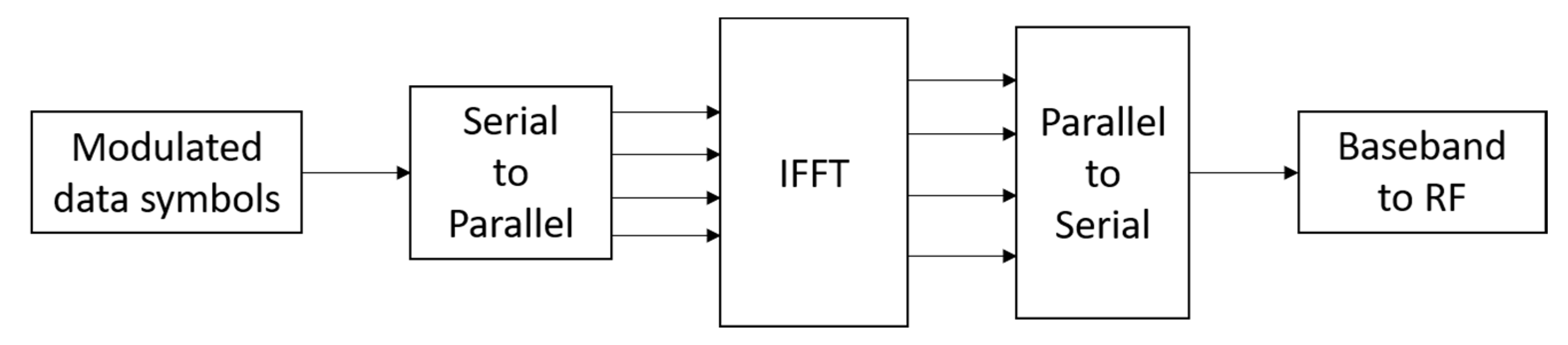
The conventional OFDM transmitter structure is implemented by combining different blocks as shown in Figure 1. After a modulation process (which is also called symbol mapping), the modulated data symbols will be converted from a serial stream to a parallel stream. In the IFFT (inverse fast Fourier transform) block, all the modulated data symbols will be carried by OFDM carriers. Subsequently, the parallel stream will be converted to a serial stream and be upconverted to transmission frequency.

There exist different variations from conventional OFDM. In order to avoid intersymbol interference (ISI), a time guard interval, such as cyclic prefix (CP) or zero padding (ZP), can be inserted between successive OFDM symbols [15]. Windowed OFDM (WOFDM), preserves the core structure of the OFDM systems with its reduced computational complexity and capability to simplify the introduction of MIMO techniques [16], which can be called as OFDM with weighted overlap and add (WOLA) [17]. At the transmitter, the edges of the rectangular pulse will be replaced by a smoother windowing function and neighboring WOLA symbols overlap, which will contribute to reduce the OOB emission of OFDM [18]. Without loss of generality, only conventional OFDM will be considered in this article.

2.2. FBMC

Unlike OFDM where the orthogonality must be ensured for all the subcarriers, FBMC only requires orthogonality for the neighboring subchannels. In addition, OFDM uses a given frequency bandwidth with subcarriers; however, FBMC divides the transmission channel into several subchannels. For exploiting the channel bandwidth, the modulation in the subchannels must adapt to the neighboring orthogonality constraint. Without the need for a cyclic prefix or a guard time [7], this method of FBMC leads to the maximum bit rate.

In recent years, FBMC has become one of the frontiers in the research for future communication systems, and many studies have shed light on the advantages of FBMC with offsite quadrature amplitude modulation (OQAM) [19]. In OQAM, the quadrature signal is delayed by T/2, where T is the symbol duration. FBMC-OQAM then multiplexes multiple subcarriers carrying OQAM data, with a $\pi /2$ phase difference between adjacent subchannels. Although OQAM is more widely used with FBMC than QAM [20], FBMC-OQAM will not be included in this article for the simplified and unified representation.

The filter bank is an array of filters, which will be applied to each of the K subcarriers, respectively. Define $v(t)$ as the prototype filter, the FBMC-QAM signal can be represented mathematically as [21]:

$$\begin{array}{cc}\hfill s\left(t\right)& ={\displaystyle \sum _{n=-\infty }^{\infty }{\displaystyle \sum _{k=0}^{K-1}{a}_{n,k}\delta (t-nT)\otimes v\left(t\right)e^{j2\pi k\Delta f\left(t-nT\right)}}}\hfill \\ & ={\displaystyle \sum _{n=-\infty }^{\infty }{\displaystyle \sum _{k=0}^{K-1}{a}_{n,k}v\left(t-nT\right)e^{j2\pi k\Delta f\left(t-nT\right)}}},\hfill \end{array}$$

(4)

While relying on dividing the spectrum into multiple subcarriers, FBMC applies a filtering functionality to each of the subcarriers in contrast to OFDM (in Figure 1) which is illustrated in Figure 2.

2.3. F-OFDM

F-OFDM now is considered as another candidate for future communication networks beyond 5G. F-OFDM still uses OFDM as its core waveform [11], and applies subband filters to each subband which has more than one subcarrier. The filter of F-OFDM should follow some of the criterion mentioned in [22] as: (1) Flat passband is the prerequisite for the subcarriers; (2) A sharp transition is a prerequisite for the filter in order to lessen the consumption of a guard band; (3) the filters requires sufficient stop band attenuation.

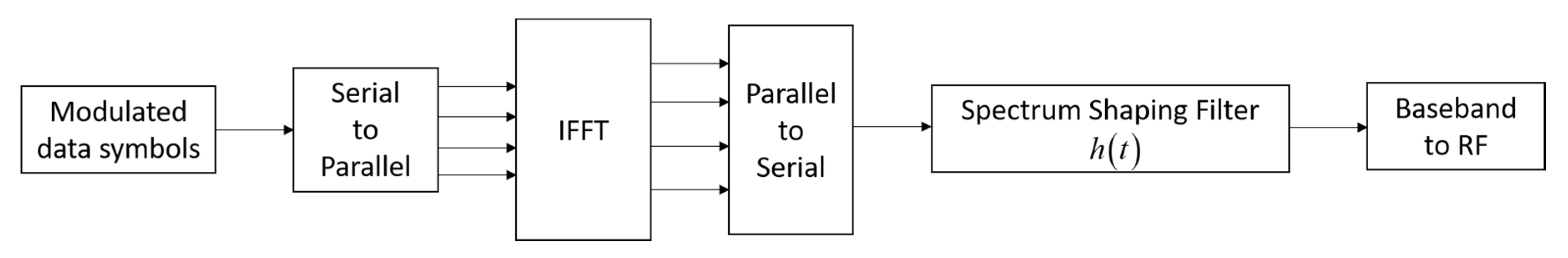
For the sake of unified expression, we assume that the spectrum shaping filter is applied to the entire passband, i.e., the total number of subbands is one. After applying an appropriately designed spectrum shaping filter $h(t)$ to the entire subband, F-OFDM transmitter structure can be illustrated in Figure 3. Other blocks of F-OFDM structure are similar to that of OFDM structure described in Figure 1.

After applying the spectrum shaping filter h(t) to the entire subband described in Equation (1), the F-OFDM signal can be derived as:

$$s\left(t\right)={\displaystyle \sum _{n=-\infty }^{\infty }{s}_n\left(t-nT\right)}={\displaystyle \sum _{n=-\infty }^{\infty }\left\{\left[{\displaystyle \sum _{k=0}^{K-1}{a}_{n,k}{e}^{j2\pi k\Delta f\left(t-nT\right)}}\right]\otimes h\left(t-nT\right)\right\}}$$

(5)

where $\otimes$ denotes the convolution operation. Based on Equations (3)–(5), a unified representation for OFDM, FBMC, and F-OFDM can be expressed as:

$$s\left(t\right)={\displaystyle \sum _{n=-\infty }^{\infty }\left\{\left[{\displaystyle \sum _{k=0}^{K-1}{a}_{n,k}v\left(t-nT\right)e^{j2\pi k\Delta f\left(t-nT\right)}}\right]\otimes h\left(t-nT\right)\right\}}$$

(6)

Equation (6) can represent OFDM, FBMC, F-OFDM signals respectively by choosing pulse shaping window $v\left(t\right)$ and spectrum shaping filter $h\left(t\right)$ appropriately. If $v\left(t\right)$ is chosen as a rectangular pulse shaping function, and $h(t)$ is chosen as $\delta (t)$, Equation (6) represents conventional OFDM signals; if $h(t)$ is chosen as $\delta (t)$, $v\left(t\right)$ could be chosen such that Equation (6) represents FBMC signals; if $v(t)$ is chosen as a rectangular pulse shaping function, $h(t)$ could be chosen such that Equation (6) represents F-OFDM signals. In the next section, based on Equation (6), a unified expression of OFDM, FBMC, and F-OFDM in frequency domain will be derived, and we will choose specific $v\left(t\right)$ and $h\left(t\right)$ for discussion.

3. Model Comparison in Frequency Domain

3.1. Unified Expression in Frequency Domain

Since $h\left(t-nT\right)$ in Equation (6) is irrelevant to k, Equation (6) can be rewritten as:

$$\begin{array}{ll}s\left(t\right)& ={\displaystyle \sum _{n=-\infty }^{\infty }\left\{\left[{\displaystyle \sum _{k=0}^{K-1}{a}_{n,k}v\left(t-nT\right)e^{j2\pi k\Delta f\left(t-nT\right)}}\right]\otimes h\left(t-nT\right)\right\}}\\ & ={\displaystyle \sum _{n=-\infty }^{\infty }\left\{{\displaystyle \sum _{k=0}^{K-1}\left[a_{n,k}v\left(t-nT\right)e^{j2\pi k\Delta f\left(t-nT\right)}\otimes h\left(t-nT\right)\right]}\right\}}\\ & ={\displaystyle \sum _{k=0}^{K-1}\left\{{\displaystyle \sum _{n=-\infty }^{\infty }\left[a_{n,k}v\left(t-nT\right)e^{j2\pi k\Delta f\left(t-nT\right)}\otimes h\left(t-nT\right)\right]}\right\}}\end{array}$$

(7)

To simplify the expression of Equation (7), two new terms are defined as:

$$s_k\left(t\right)={\displaystyle \sum _{n=-\infty }^{\infty }{a}_{n,k}v\left(t-nT\right)e^{j2\pi k\Delta f\left(t-nT\right)}\otimes h\left(t-nT\right)}$$

(8)

$$g_k\left(t\right)=v\left(t\right)e^{j2\pi k\Delta ft}\otimes h\left(t\right)$$

(9)

Thus, Equation (7) can be rewritten as:

$$s\left(t\right)={\displaystyle \sum _{k=0}^{K-1}{s}_k\left(t\right)}={\displaystyle \sum _{k=0}^{K-1}{\displaystyle \sum _{n=-\infty }^{\infty }{a}_{n,k}{g}_k\left(t-nT\right)}}$$

(10)

Taking a Fourier transform on both sides of Equation (10) will yield:

$$S\left(f\right)=\mathfrak{F}\left\{s\left(t\right)\right\}=\mathfrak{F}\left\{{\displaystyle \sum _{k=0}^{K-1}{s}_k\left(t\right)}\right\}={\displaystyle \sum _{k=0}^{K-1}{S}_k\left(f\right)},$$

(11)

where $\mathfrak{F}\{\cdot \}$ stands for the Fourier transform operation of $\{\cdot \}$, e.g., $\mathfrak{F}\left\{s\left(t\right)\right\}=S\left(f\right)$ is the Fourier transform of signal $s\left(t\right)$. Based on Equations (8)–(10), $S_k\left(f\right)$ can be derived as:

$$\begin{array}{ll}{S}_k\left(f\right)& =\mathfrak{F}\left\{s_k\left(t\right)\right\}=\mathfrak{F}\left\{{\displaystyle \sum _{n=-\infty }^{\infty }{a}_{n,k}{g}_k\left(t-nT\right)}\right\}\\ & ={\displaystyle \sum _{n=-\infty }^{\infty }{a}_{n,k}\mathfrak{F}\left\{g_k\left(t-nT\right)\right\}}\\ & ={\displaystyle \sum _{n=-\infty }^{\infty }{a}_{n,k}{G}_k\left(f\right)e^{-j2\pi fnT}},\end{array}$$

(12)

where $G_k\left(f\right)$ is the Fourier transform of $g_k\left(t\right)$. With Equation (12), the PSD (Power spectrum density) of $s\left(t\right)$ can be derived as [23]:

$$\begin{array}{l}{P}_s\left(f\right)=\underset{T\to \infty }{\lim }\frac{E\left\{S\left(f\right)S^{*}\left(f\right)\right\}}{T}\\ =\underset{T\to \infty }{\lim }\frac{1}{T}E\left\{\left[{\displaystyle \sum _{k=0}^{K-1}{S}_k\left(f\right)}\right]\left[{\displaystyle \sum _{k=0}^{K-1}{S}_k^{*}\left(f\right)}\right]\right\}\\ =\underset{T\to \infty }{\lim }\frac{1}{T}E\left\{{\displaystyle \sum _{k_1=0}^{K-1}{\displaystyle \sum _{k_2=0}^{K-1}{S}_{k_1}\left(f\right)S_{k_2}^{*}\left(f\right)}}\right\}\\ =\underset{T\to \infty }{\lim }\frac{1}{T}E\left\{{\displaystyle \sum _{k_1=0}^{K-1}{\displaystyle \sum _{k_2=0}^{K-1}{\displaystyle \sum _{n_1=-\infty }^{\infty }{\displaystyle \sum _{n_2=-\infty }^{\infty }\left[a_{n_1,k_1}{a}_{n_2,k_2}^{*}{G}_{k_1}\left(f\right)G_{k_2}^{*}\left(f\right)e^{-j2\pi f\left(n_1-n_2\right)T}\right]}}}}\right\}\\ =\underset{T\to \infty }{\lim }\frac{1}{T}{\displaystyle \sum _{k_1=0}^{K-1}{\displaystyle \sum _{k_2=0}^{K-1}{\displaystyle \sum _{n_1=-\infty }^{\infty }{\displaystyle \sum _{n_2=-\infty }^{\infty }\left[E\left\{a_{n_1,k_1}{a}_{n_2,k_2}^{*}\right\}{G}_{k_1}\left(f\right)G_{k_2}^{*}\left(f\right)e^{-j2\pi f\left(n_1-n_2\right)T}\right]}}}}\end{array}$$

(13)

Since the transmitted data symbol $a_{n,k}$ is orthogonal for different n and k, we then have [24]:

$$E\left\{a_{n_1,k_1}{a}_{n_2,k_2}^{*}\right\}=\{\begin{array}{ll}{\sigma }_a^2,\hfill & \mathrm{if} n_1=n_2 \mathrm{and} k_1=k_2\hfill \\ 0,\hfill & \mathrm{otherwise}\hfill \end{array}$$

(14)

where $E\{\cdot \}$ donates the mathematical expectation of $\{\cdot \}$, and ${\sigma }_a$ is the standard derivation of $a_{n,k}$ As $k_1=k_2$, we will use k instead. Thus, Equation (13) can be further derived as:

$$\begin{array}{l}{P}_s\left(f\right)\\ =\underset{T\to \infty }{\lim }\frac{1}{T}{\displaystyle \sum _{k_1=0}^{K-1}{\displaystyle \sum _{k_2=0}^{K-1}{\displaystyle \sum _{n_1=-\infty }^{\infty }{\displaystyle \sum _{n_2=-\infty }^{\infty }\left[E\left\{a_{n_1,k_1}{a}_{n_2,k_2}^{*}\right\}{G}_{k_1}\left(f\right)G_{k_2}^{*}\left(f\right)e^{-j2\pi f\left(n_1-n_2\right)T}\right]}}}}\\ =\underset{T\to \infty }{\lim }\frac{1}{T}\{{\displaystyle \sum _{k=0}^{K-1}{\displaystyle \sum _{n_1=-\infty }^{\infty }{\displaystyle \sum _{n_2=-\infty }^{\infty }\left[E\left\{a_{n_1,k}{a}_{n_2,k}^{*}\right\}{G}_k\left(f\right)G_k^{*}\left(f\right)e^{-j2\pi f\left(n_1-n_2\right)T}\right]}}}\\ +\underset{\mathrm{equals}\mathrm{to}0}{\underbrace{{\displaystyle \sum _{k_1=0}^{K-1}{\displaystyle \sum _{k_2\ne k_1}^{K-1}{\displaystyle \sum _{n_1=-\infty }^{\infty }{\displaystyle \sum _{n_2=-\infty }^{\infty }\left[E\left\{a_{n_1,k_1}{a}_{n_2,k_2}^{*}\right\}{G}_{k_1}\left(f\right)G_{k_2}^{*}\left(f\right)e^{-j2\pi f\left(n_1-n_2\right)T}\right]}}}}}}\}\\ =\underset{T\to \infty }{\lim }\frac{1}{T}{\displaystyle \sum _{k=0}^{K-1}E\left\{{\displaystyle \sum _{n_1=-\infty }^{\infty }{\displaystyle \sum _{n_2=-\infty }^{\infty }\left[a_{n_1,k}{a}_{n_2,k}^{*}{G}_k\left(f\right)G_k^{*}\left(f\right)e^{-j2\pi f\left(n_1-n_2\right)T}\right]}}\right\}}\\ =\underset{T\to \infty }{\lim }\frac{1}{T}{\displaystyle \sum _{k=0}^{K-1}E\left\{S_k\left(f\right)S_k^{*}\left(f\right)\right\}}\\ ={\displaystyle \sum _{k=0}^{K-1}{P}_{s_k}\left(f\right)}\end{array}$$

(15)

where $P_{s_k}\left(f\right)$ is the PSD of $s_k\left(t\right)$. The derivation of Equation (15) proved that the overall spectrum is the sum of the spectra at each subcarrier. This enables us to derive further. By substituting Equation (9) into Equation (8), $s_k\left(t\right)$ can be derived as:

$$s_k\left(t\right)={\displaystyle \sum _{n=-\infty }^{\infty }{a}_{n,k}{g}_k\left(t-nT\right)}$$

(16)

With the similar method in [23], $P_{s_k}\left(f\right)$ can be derived as:

$$P_{s_k}\left(f\right)=\frac{{\sigma }_a^2}{T}{\left|G_k\left(f\right)\right|}^2$$

(17)

In Equation (17), $G_k\left(f\right)$ can be derived as:

$$G_k\left(f\right)=\mathfrak{F}\left\{g_k\left(t\right)\right\}=V\left(f-k\Delta f\right)H\left(f\right),$$

(18)

where $V\left(f\right)$ and $H\left(f\right)$ are the Fourier transform of $v\left(t\right)$ and $h\left(t\right)$, respectively. By substituting Equation (18) into Equation (17), $P_{s_k}\left(f\right)$ can be derived as:

$$P_{s_k}\left(f\right)=\frac{1}{T}{\sigma }_a^2{\left|V\left(f-k\Delta f\right)H\left(f\right)\right|}^2.$$

(19)

Therefore, with Equation (15) and Equation (19), $P_s\left(f\right)$ can be expressed as:

$$P_s\left(f\right)=\frac{{\left|H\left(f\right)\right|}^2{\sigma }_a^2}{T}{\displaystyle \sum _{k=0}^{K-1}{\left|V\left(f-k\Delta f\right)\right|}^2}.$$

(20)

Equation (20) is a unified expression of power spectrum for OFDM, FBMC, and F-OFDM signals. It could be specified for OFDM, FBMC, or F-OFDM by selecting spectrum shaping filter $H\left(f\right)$ and pulse shaping window V(f). The following Section 3.2, Section 3.3, Section 3.4 will discuss how to use Equation (20) in different multicarrier modulation techniques.

3.2. OFDM

For conventional OFDM, $v(t)$ in Equation (6) is a rectangular pulse such that $V(f)$ in Equation (20) can be expressed as [25]:

$$V\left(f\right)=T\mathrm{sinc}\left(Tf\right)=\frac{T\sin (\pi Tf)}{\pi Tf}$$

(21)

Since the filter $H\left(f\right)$ in Equation (20) is not used in the conventional OFDM, the magnitude of $H\left(f\right)$ is then assumed as a unity constant. Thus, substituting Equation (21) into Equation (20), the PSD of the conventional OFDM signals can be derived as:

$$\begin{array}{ll}{P}_s\left(f\right)& =\frac{{\sigma }_a^2}{T}{\displaystyle \sum _{k=0}^{K-1}{\left|T\mathrm{sinc}\left[T\left(f-k\Delta f\right)\right]\right|}^2}\\ & =T{\sigma }_a^2{\displaystyle \sum _{k=0}^{K-1}{\left|\mathrm{sinc}\left[T\left(f-k\Delta f\right)\right]\right|}^2}\end{array}$$

(22)

3.3. FBMC

As shown in Figure 2, a filter is applied to each of the subcarriers in FBMC approach. A variety of prototype filter options for FBMC systems is summarized in [26]. The most popular prototype filters are extended gaussian function (EGF) [27,28], Martin-Mirabbasi [10,29] and optimal finite duration pulses (OFDP) [30,31], due to their remarkable features and simplicity. Other options include the windowed based prototype filter [32], the Hermite filter discussed in [33], and the classical square-root raised cosine [16]. Also, some recent work could be found in [34,35].

PHYDYAS prototype filter, a special case of Mirabbasi-Martin filter when the overlapping factor I is 4, has gained the prominence as it is chosen for the PHYDYAS project [36] and also used in FBMC examples in communications toolbox in the MATLAB [37], thus we will use this PHYDYAS filter in this article.

The frequency response of PHYDYAS filter can be shown as [36]:

$$V\left(f\right)={\displaystyle \sum _{i=-\left(I-1\right)}^{I-1}{L}_i\frac{\sin \left[\pi \left(f-\frac{i}{KI}\right)KI\right]}{KI\sin \left[\pi \left(f-\frac{i}{KI}\right)\right]}}\left(I=4\right),$$

(23)

where $L_i$ denotes the coefficient of PHYDYAS filter as shown in

Table 1. Mirabbasi-Martin Filter Coefficients as I = 4 for PHYDYAS.

I	$L_0$	$L_1$	$L_2$	$L_3$	…
…	…	…	…	…	…
4	1	0.971960	$\raisebox{1ex}{$\sqrt{2}$}\!\left/ \!\raisebox{-1ex}{$2$}\right.$	0.235147	-
…	…	…	…	…	…

.

By substituting Equation (23) into Equation (20), and considering $H\left(f\right)$ as constant one, the PSD of FBMC signal can be derived as:

$$P_s\left(f\right)=\frac{{\sigma }_a^2}{T}{\displaystyle \sum _{k=0}^{K-1}{\left|{\displaystyle \sum _{i=-\left(I-1\right)}^{I-1}{L}_i\frac{\sin \left[IK\pi \left(f-\frac{i}{IK}-\frac{k}{K}\right)\right]}{IK\sin \left[\pi \left(f-\frac{i}{IK}-\frac{k}{K}\right)\right]}}\right|}^2}$$

(24)

With the choice that $I=4$, Equation (24) can be further expressed as:

$$P_s\left(f\right)=\frac{{\sigma }_a^2}{T}{{\displaystyle \sum _{k=0}^{K-1}\left|{\displaystyle \sum _{i=-3}^3{L}_i\frac{\sin \left[4K\pi \left(f-\frac{i}{4K}-\frac{k}{K}\right)\right]}{4K\sin \left[\pi \left(f-\frac{i}{4K}-\frac{k}{K}\right)\right]}}\right|}}^2$$

(25)

Equation (25) will be used in our numerical calculation in Section 3.5.

3.4. F-OFDM

The PSD of F-OFDM can be described as:

$$P_s\left(f\right)={\left|H\left(f\right)\right|}^{2}T{\sigma }_a^2{\displaystyle \sum _{k=0}^{K-1}{\left|\mathrm{sinc}\left[T\left(f-k\Delta f\right)\right]\right|}^2}.$$

(26)

In order to choose an appropriate filter $H\left(f\right)$ for F-OFDM, the criterion mentioned in Section 2.3 should be satisfied. In [38], a truncated filter, a window function $w(t)$ applied on an impulse response ${\sin \mathrm{c}}_B\left(t\right)$, is proposed as:

$$h\left(t\right)={\sin \mathrm{c}}_B\left(t\right)w\left(t\right),$$

(27)

where the bandwidth of the sinc impulse response is B. Substituting Equation (27) into Equation (26), the PSD of F-OFDM can then be derived as:

$$P_s\left(f\right)={\left|\mathrm{rect}\left(\frac{f}{2B}\right)\otimes W(f)\right|}^{2}T{\sigma }_a^2{\displaystyle \sum _{k=0}^{K-1}{\left|\mathrm{sinc}\left[T\left(f-k\Delta f\right)\right]\right|}^2},$$

(28)

In Equation (27), w(t) has smooth transitions to zero on both ends to avoid abrupt jumps at the beginning and end of the truncated filter, hence avoiding the frequency spillover in the truncated filter. In [39], the applied window $w(t)$ is given by:

$$w(t)=\{\begin{array}{cc}0.5{[1+\cos (2\pi t/T_w)]}^{\alpha },& \left|t\right|\le \frac{T_w}{2}\\ 0,& \left|t\right|>\frac{T_w}{2}\end{array}.$$

(29)

where $\alpha$ is the roll-off factor used to control the shape of the window, and $T_w$ is the filter length. The freedom of $\alpha$ contributes to a better balance between time and frequency localization. Let $\alpha =0$, it is simply a rectangular window; $\alpha =0.6$ was considered by the 3GPP workgroups [40]; if $\alpha =1$, it becomes a Hann window [38] which can be expressed as:

$$w_H(t)=\{\begin{array}{cc}0.5[1+\cos (2\pi t/T_w)],& \left|t\right|\le \frac{T_w}{2}\\ 0,& \left|t\right|>\frac{T_w}{2}\end{array}.$$

(30)

Equation (30) can then be rewritten as:

$$\begin{array}{ll}{w}_H(t)& =\frac{1}{2}[1+\cos (2\pi t/T_w)]\mathrm{rect}(t/T_w)\\ & =\frac{1}{2}\mathrm{rect}(t/T_w)+\frac{1}{2}\cos (\frac{2\pi t}{T_w})\mathrm{rect}(t/T_w)\\ & =\frac{1}{2}\mathrm{rect}(t/T_w)+\frac{1}{4}{e}^{j2\pi t/T_w}\mathrm{rect}(t/T_w)\\ & +\frac{1}{4}{e}^{-j2\pi t/T_w}\mathrm{rect}(t/T_w)\end{array}$$

(31)

Taking a Fourier transform yields:

$$\begin{array}{ll}{W}_H(f)& =\frac{1}{2}\frac{\sin (\pi T_{w}f)}{\pi f}+\frac{1}{4}\frac{\sin (\pi T_w(f-1/T_w))}{\pi (f-1/T_w)}\\ & +\frac{1}{4}\frac{\sin (\pi T_w(f+1/T_w))}{\pi (f+1/T_w)}\end{array}$$

(32)

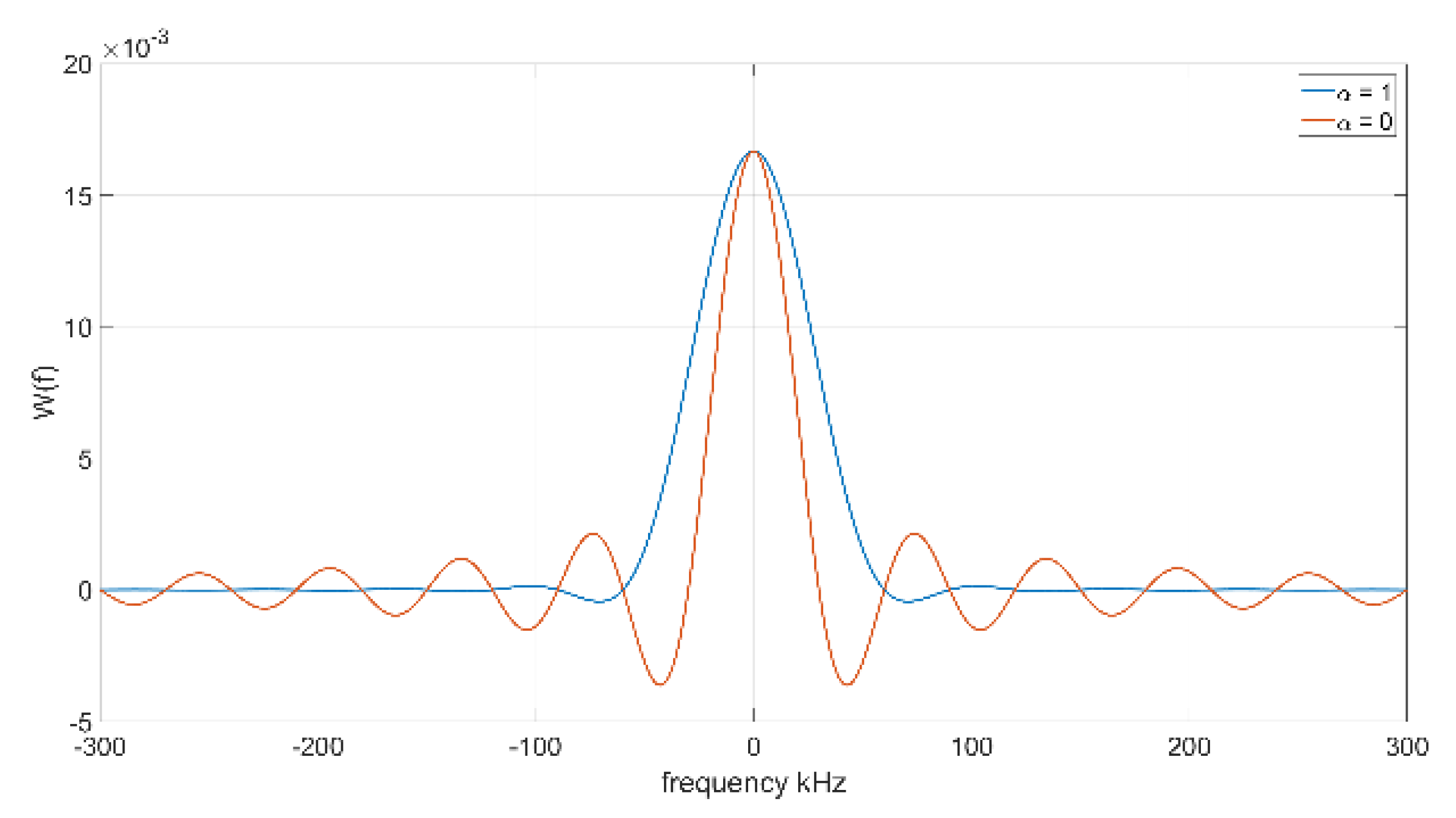
The first term in Equation (32) contributes most to the main lobe, and the second and third terms contribute to doubling the null bandwidth and smoothing the sidelobe, which is shown is Figure 4. Hann window $W_H(f)$ in Equation (32) will be used in our calculation in next section. Figure 4 describes the window function $w(t)$ in frequency domain as $\alpha =0$ and $\alpha =1$, respectively.

3.5. Comparison among OFDM, FBMC, and F-OFDM

Table 2. Our choices of $v\left(t\right)$ and $h\left(t\right)$ for OFDM, FBMC, and F-OFDM.

I	OFDM	FBMC	F-OFDM
$v\left(t\right)$	Rectangular pulse shaping	PHYDYAS etc.	Rectangular pulse shaping
$h\left(t\right)$	-	-	Truncated filter with Hann window

summarizes our choices of $v\left(t\right)$ and $h\left(t\right)$ for OFDM, FBMC, and F-OFDM, respectively. Among all the options/varieties of pulse shaping filters $v\left(t\right)$ and spectrum shaping filters $h\left(t\right)$ described in the previous sections, our choices are summarized in Table 2.

With the different choices of $v\left(t\right)$ or $h\left(t\right)$ for OFDM, FBMC, and F-OFDM, we could predict the spectra of these three signals to compare their OOB emissions. In OFDM systems, $v\left(t\right)$ is chosen as a rectangular pulse shaping, which results in a sinc spectrum in frequency domain. The side lobes of the sinc spectrum will produce overlapping spectra among subcarriers. As a result, the interference among subcarriers dramatically increases the OOB emission of the combined spectra.

For FBMC signals, $v\left(t\right)$ is chosen as a PHYDYAS filter. The frequency response of PHYDYAS filter is shown in Equation (23). The out-of-band ripples of the FBMC subcarrier are extremely small, which will nearly disappear after several ripples, thus the PHYDYAS filter can be considered as a highly selective filter [36]. Due to the low side lobe property of each FBMC subcarrier, the interference of subcarriers is neglectable so that the OOB emission of the combined spectra is small.

For F-OFDM signals, a well-designed truncated subband filter will be applied to the conventional OFDM signal to reduce the OOB emission. In this article, h(t) is chosen as a truncated filter with Hann window as Equations (27) and (30). Since F-OFDM uses OFDM as its core waveform, v(t) is chosen as rectangular pulse shaping as well. After applying the truncated filter to conventional OFDM, the OOB emission of the F-OFDM spectrum is improved comparing with that of conventional OFDM signals.

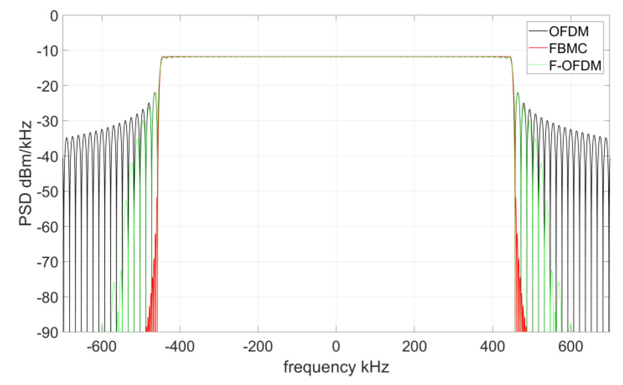
A comparison of OFDM, FBMC, and F-OFDM, based on Equations (22), (25), and (28) with Equation (32), in terms of PSD is shown in Figure 5. The frequency space of subcarriers is chosen as 15 kHz, and the number of subcarriers is chosen as 60. The black line represents the OFDM signals, the green line represents F-OFDM signals, and the red line represents FBMC signals. Due to the half-Nyquist filter used in Equation (25), we can see that FBMC has much better spectral performance compared to OFDM and F-OFDM. Also, the OOB emission of F-OFDM will dramatically decrease after few side lobes, due to the Hann window used in Equation (28). It can be seen that the V(f) and H(f) in Equation (20) make significant contributions for reducing OOB emission.

4. Empirical Sideband Quantification

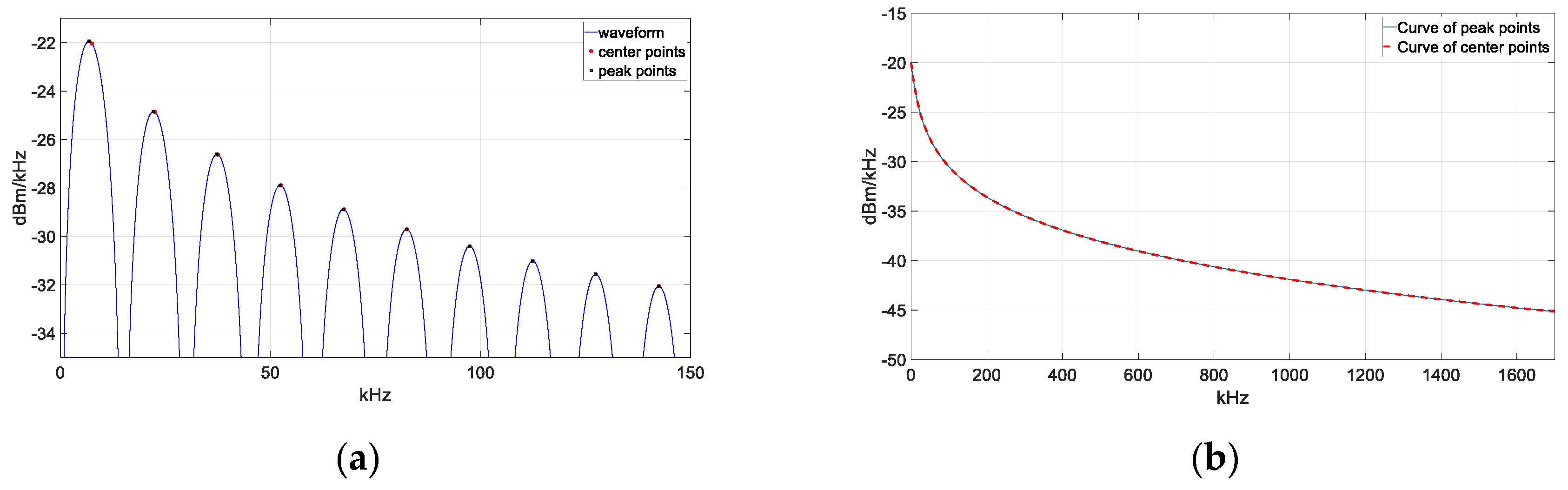
Spectrum emission mask (SEM), as defined in 3GPP TS 34.122 [41], is a relative measurement of the out-of-channel emissions and the in-channel power. So as to meet the requirements of OOB emission mask, the side lobes must be lower than the limit lines of the emission mask. However, it is difficult to derive a closed form of the side lobes as the peak points are hard to calculate. Thus, an empirical quantification method is used to estimate the side lobes, using the center points to replace the peak points, to simplify the calculation.

In Figure 6a, the blue line traces the side lobes to the right of the OFDM passband. The black dots are the peak points of side lobes, and the red circles are the center points of side lobes. For each side lobe, the difference between the peak point and the center point is negligibly small, which is verified by the magnitude differences in

Table 3. Magnitude difference between the peak points and center points of the first nine side lobes in Figure 6a.

Title 1	Point 1	Point 2	Point 3	Point 4	Point 5	Point 6	Point 7	Point 8	Point 9
Nth peak points (dBm)	−21.94	−24.85	−26.61	−27.88	−28.88	−29.70	−30.406	−31.019	−31.563
Nth peak points (dBm)	−22.04	−24.87	−26.62	−27.89	−28.89	−29.71	−30.408	−31.021	−31.565
Difference (dB)	0.1	0.02	0.01	0.01	0.01	0.01	0.002	0.002	0.002

. In addition, the trend of differences rapidly decreases as the index n increases. Figure 6b illustrates the spectral envelope of peak points (blue solid line) and that of center points (red dashed line) up to 1500 kHz.

It can be observed that the two spectral envelopes nearly overlap with each other. Thus, in this article, the center points are empirically used to replace the peak points to estimate the envelope. Based on this empirical assumption and Equation (22), the PSD of the center point for the q-th side lobe, P(f_q) $f_q=(-2q-1/2)\Delta f$), can be derived as:

$$\begin{array}{ll}P\left(f_q\right)& =T{\sigma }_a^2{\displaystyle \sum _{k=0}^{K-1}{\left|\mathrm{sinc}\left[T\left(f_q-k\Delta f\right)\right]\right|}^2}\\ & =T{\sigma }_a^2{\displaystyle \sum _{k=0}^{K-1}{\left|\mathrm{sinc}\left[T\left(\frac{2q+1+2k}{2}\Delta f\right)\right]\right|}^2}\\ & =T{\sigma }_a^2{\displaystyle \sum _{k=0}^{K-1}{\left|\frac{\sin \left[\pi T\left(\frac{2q+1+2k}{2}\right)\Delta f\right]}{\pi T\left(\frac{2q+1+2k}{2}\Delta f\right)}\right|}^2}\\ & =T{\sigma }_a^2{\displaystyle \sum _{k=0}^{K-1}{\left|\frac{\sin \left[\left(q+k+\frac{1}{2}\right)\pi \right]}{\pi T\left(\frac{2q+1+2k}{2}\Delta f\right)}\right|}^2}\\ & =T{\sigma }_a^2{\displaystyle \sum _{k=0}^{K-1}\frac{1}{{\left[\pi T\left(\frac{2q+1+2k}{2}\Delta f\right)\right]}^2}}\\ & =\frac{4{\sigma }_a^{2}T}{{\pi }^2}{\displaystyle \sum _{k=0}^{K-1}\frac{1}{{\left(2k+2q+1\right)}^2}}\end{array}$$

(33)

If the number of subcarriers K approaches to infinity, Equation (33) becomes:

$$P\left(f_q\right)=\frac{4{\sigma }_a^{2}T}{{\pi }^2}{\displaystyle \sum _{k=0}^{\infty }\frac{1}{{\left(2k+2q+1\right)}^2}}$$

(34)

In Equation (34), ${\displaystyle \sum _{k=0}^{\infty }\frac{1}{{\left(2k+2q+1\right)}^2}}$ could be rewritten as $\left[{\displaystyle \sum _{k=0}^{\infty }\frac{1}{{\left(2k+1\right)}^2}}-{\displaystyle \sum _{j=0}^{q-1}\frac{1}{{\left(2j+1\right)}^2}}\right]$. With the fact that ${\displaystyle \sum _{k=0}^{\infty }\frac{1}{{\left(2k+1\right)}^2}=\frac{8}{\pi }}$ [42], Equation (34) can then be rewritten as:

$$P\left(f_q\right)=\frac{4{\sigma }_a^{2}T}{{\pi }^2}\left[{\displaystyle \sum _{k=0}^{\infty }\frac{1}{{\left(2k+1\right)}^2}}-{\displaystyle \sum _{j=0}^{q-1}\frac{1}{{\left(2j+1\right)}^2}}\right]=\frac{4{\sigma }_a^{2}T}{{\pi }^2}\left[\frac{{\pi }^2}{8}-{\displaystyle \sum _{j=0}^{q-1}\frac{1}{{\left(2j+1\right)}^2}}\right]$$

(35)

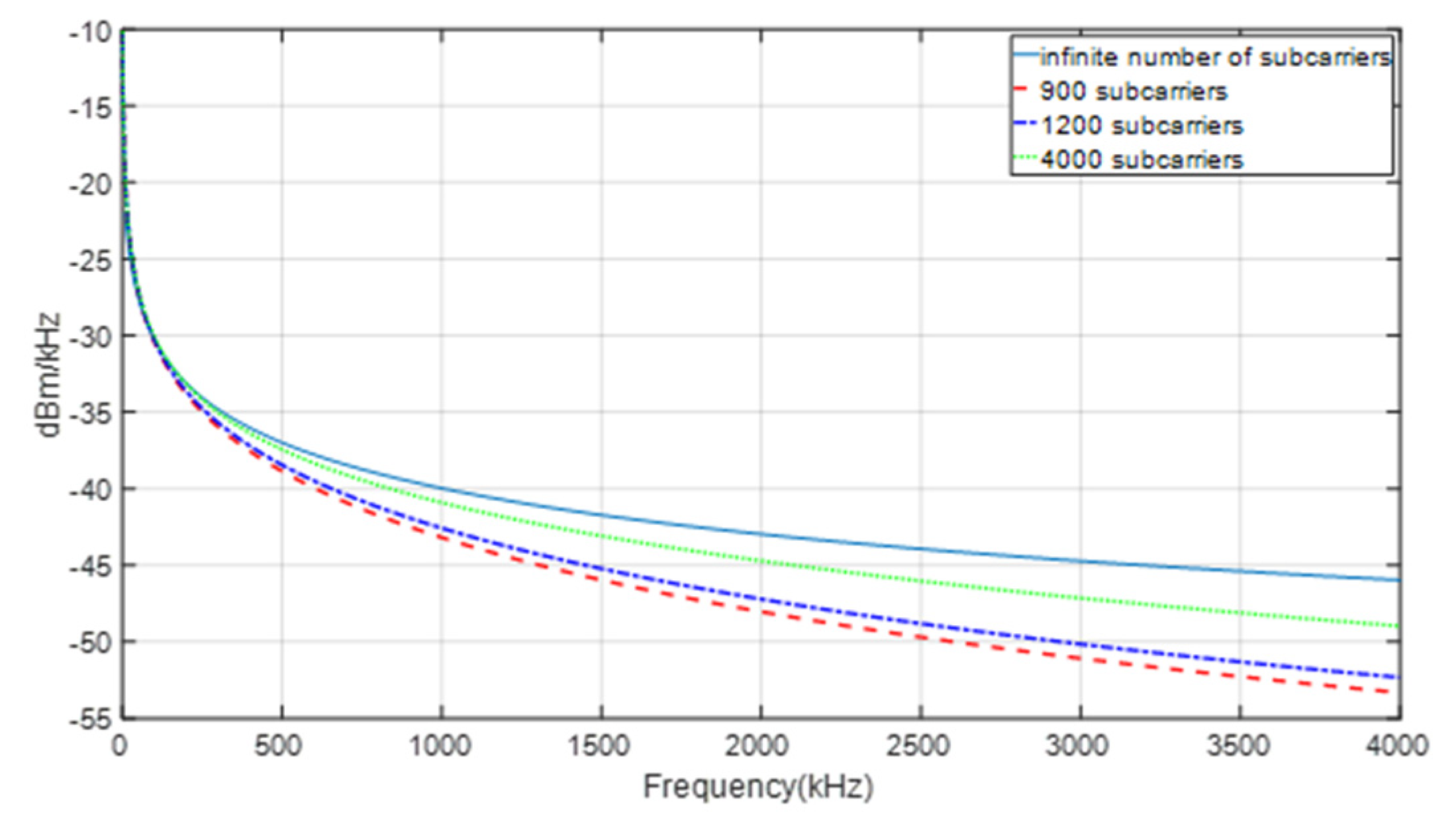
In Figure 7, the green dotted waveform describes the spectral envelope of maximum points in OFDM modulation with 4000 subcarriers, the blue dash-dot waveform describes the spectral envelope of maximum points in OFDM modulation with 1200 subcarriers, the red dashed waveform describes the spectral envelope of maximum points in OFDM modulation with 900 subcarriers, and the cyan solid waveform describes the envelope of this empirical model as the number of subcarriers goes to infinity (q is chosen as 900). As the number of subcarriers increases, the spectral envelope approaches to the limit of the spectral envelope. Therefore, Equation (35) can be used for an upper bound limit for the spectrum of OFDM signals.

In addition, based on Equations (28) and (35), the upper bound limit of F-OFDM signals for q-th side lobe can be derived as:

$$P\left(f_q\right)={\left|H\left(f_q\right)\right|}^2\frac{4{\sigma }_a^{2}T}{{\pi }^2}\left[\frac{{\pi }^2}{8}-{\displaystyle \sum _{j=0}^{q-1}\frac{1}{{\left(2j+1\right)}^2}}\right]$$

(36)

It can be seen that the filter $H\left(f_q\right)$ significantly decreases the OOB emission in Figure 5.

5. Practical Consideration

The pulse shaping window $v(t)$ in Equation (6) is practically obtained from sampled pulse shaping window $v^{\prime }\left[n\right]$ by using a perfect brick-wall interpolation filter [15] as:

$$v\left(t\right)={\displaystyle \sum _{n=-\infty }^{\infty }{v}^{\prime }\left[n\right]g_I\left(t-n{T}_s\right)}$$

(37)

where $g_I\left(t\right)$ is the interpolation filter, and $T_s$ is the sampling interval employed in the OFDM transmitter.

Since $v^{\prime }\left[n\right]$ are the samples from the original pulse shaping window $v^{\prime }\left(t\right)$, Equation (37) can be rewritten as:

$$v\left(t\right)={\displaystyle \sum _{n=-\infty }^{\infty }{v}^{\prime }\left[n\right]g_I\left(t-n{T}_s\right)}={\displaystyle \sum _{n=-\infty }^{\infty }{v}^{\prime }\left(n{T}_s\right)\delta \left(t-n{T}_s\right)}\otimes g_I\left(t\right)=\left[{\displaystyle \sum _{n=-\infty }^{\infty }{v}^{\prime }\left(t\right)\delta \left(t-n{T}_s\right)}\right]\otimes g_I\left(t\right)$$

(38)

The frequency response of pulse shaping window V(f) can be obtained as:

$$V\left(f\right)=\mathfrak{F}\left\{v\left(t\right)\right\}=\left[{\displaystyle \sum _{n=-\infty }^{\infty }{v}^{\prime }\left(f-n f_s\right)}\right]G_I\left(f\right)$$

(39)

where $v^{\prime }\left(f\right)=\mathfrak{F}\left\{v^{\prime }\left(t\right)\right\}$ is the frequency response of $v^{\prime }\left(t\right)$, $G_I\left(f\right)=\mathfrak{F}\left\{g_I\left(t\right)\right\}$ is the frequency response of $g_I\left(t\right)$, and $f_s=1/T_s$ is the sampling frequency.

If $v^{\prime }\left(t\right)$ is bandlimited and the sampling process satisfies Nyquist theorem, the reconstructed spectrum of the sampled pulse shaping window is identical to that of the continuous pulse shaping window; if $v^{\prime }\left(t\right)$ is not bandlimited, there exist aliases in spectrum within V(f), we will include this situation into the unified analysis in our future research.

6. Conclusions

In this article, a unified spectrum formulation for the OFDM, FBMC and F-OFDM signals has been developed. In a common spectrum framework, we can clearly see the performance differences such as OOB emission due to the different choices of the various pulse shaping or spectrum shaping filters, respectively. Finally, an empirical quantification for the sideband envelope is presented, which can be used as an upper bound limit for OOB emission measurements.

References

- Chen, W.Y. DSL: Simulation Techniques and Standards Development for Digital Subscriber Line Systems, 1st ed.; Macmillan Technical Pub.: London, UK, 1998. [Google Scholar]
- Cioffi, J.; Silverman, P.; Starr, T. Understanding Digital Subscriber Line Technology, 1st ed.; Prentice Hall: Bergen County, NJ, USA, 1999. [Google Scholar]
- Li, Y.; Stüber, G. Orthogonal Frequency Division Multiplexing for Wireless Communications, 2006th ed.; Springer: New York, NY, USA, 2006. [Google Scholar]
- Farhang Boroujeny, B.; Moradi, H. OFDM inspired waveforms for 5G. IEEE Trans. Commun. Surv. Tutor. 2016, 18, 2474–2492. [Google Scholar] [CrossRef]
- 3GPP. Study on New Radio Access Technology Radio Interface Protocol Aspects. (Release 14). Available online: http://www.3gpp.org/DynaReport/38804.htm (accessed on 19 June 2020).
- 3GPP. Study on New Radio Access Technology Physical Layer Aspects. (Release 14). Available online: http://www.3gpp.org/DynaReport/38802.htm (accessed on 19 June 2020).
- Nee, R.V.; Prasad, R. OFDM for Wireless Multimedia Communications; Artech House: Suburban Boston, MA, USA, 2000. [Google Scholar]
- Ankarali, Z.; Pekoz, B.; Arslan, H. Flexible radio access beyond 5G: A future projection on waveform, numerology, and frame design principles flex. IEEE Access 2017, 5, 18295–18309. [Google Scholar] [CrossRef]
- Zhang, L.; Ijaz, A.; Xiao, P.; Molu, M. Filtered OFDM systems, algorithms, and performance analysis for 5G and beyond. IEEE Trans. Commun. 2018, 66, 1205–1218. [Google Scholar] [CrossRef] [Green Version]
- Nissel, R.; Schwarz, S.; Moradi, H. Filter bank multicarrier modulation schemes for future mobile communications. IEEE J. Sel. Areas Commun. 2017, 35, 1768–1782. [Google Scholar] [CrossRef]
- Farhang-Boroujeny, B. OFDM versus filter bank multicarrier. IEEE Signal Process. Mag. 2011, 28, 92–112. [Google Scholar] [CrossRef]
- Rajabzadeh, M.; Steendam, H. Power spectral analysis of UW-OFDM systems. IEEE Trans. Commun. 2018, 66, 2685–2695. [Google Scholar] [CrossRef]
- 3GPP. Evolved Universal Terrestrial Radio Access (E-UTRA) Physical Channels and Modulation. Available online: http://www.3gpp.org/DynaReport/36211.htm (accessed on 19 June 2020).
- Zaidi, A.; Athley, F.; Medbo, J.; Gustavsson, U.; Durisi, G.; Chen, X. 5G Physical Layer: Principles, Models and Technology Components; Academic Press: London, UK, 2018. [Google Scholar]
- Waterschoot, T.; Le Nir, V.; Duplicy, J.; Moonen, M. Analytical expressions for the power spectral density of CP-OFDM and ZP-OFDM signals. IEEE Signal Process. Lett. 2010, 17, 371–374. [Google Scholar] [CrossRef]
- Farhang-Boroujeny, B.; Yuen, C. Cosine modulated and offset QAM filter bank multicarrier techniques: A continuous-time prospect. EURASIP J. Adv. Signal Process. 2010, 2010, 1–16. [Google Scholar] [CrossRef] [Green Version]
- Mattera, D.; Tanda, M. Windowed OFDM for small-cell 5G uplink. Phys. Commun. 2020, 39, 100993. [Google Scholar] [CrossRef]
- Mizutani, K.; Matsumura, T.; Harada, H. A Comprehensive Study of Universal Time-Domain Windowed OFDM-Based LTE Downlink System. In Proceedings of the 2017 20th International Symposium on Wireless Personal Multimedia Communications (WPMC), Bali, Indonesia, 17–20 December 2017; pp. 28–34. [Google Scholar] [CrossRef]
- Zhao, J. DFT-based offset-QAM OFDM for optical communications. Opt. Express 2014, 22, 1114–1126. [Google Scholar] [CrossRef] [PubMed]
- Moles-Cases, V.; Zaidi, A.; Chen, X.; Oechtering, T.; Baldemair, R. A Comparison of OFDM, QAM-FBMC, and OQAM-FBMC. In Proceedings of the 2017 IEEE International Conference on Communications (ICC), Paris, France, 21–25 May 2017. [Google Scholar] [CrossRef]
- Luo, F.; Zhang, C. Signal Processing for 5G: Algorithm and Implementations, 1st ed.; John Wiley & Sons Ltd.: West Sussex, UK, 2016. [Google Scholar]
- Jayan, G.; Nair, A.K. Performance Analysis of Filtered OFDM for 5G. In Proceedings of the 2018 International Conference on Wireless Communications, Signal Processing and Networking (WiSPNET), Chennai, India, 22–24 March 2018; pp. 1–5. [Google Scholar] [CrossRef]
- Couch, L.W. Digital and Analog Communication System, 7th ed.; Pearson: New York, NY, USA, 2007. [Google Scholar]
- Talbot, S.L.; Farhang-Boroujeny, B. Spectral Method of Blind Carrier Tracking for OFDM. IEEE Trans. Signal Process. 2008, 56, 2706–2717. [Google Scholar] [CrossRef]
- Proakis, J.G.; Salehi, M. Communication Systems Engineering; Prentice-Hall: Bergen County, NJ, USA, 2002. [Google Scholar]
- Kobayashi, R.T.; Abrão, T. FBMC Prototype Filter Design via Convex Optimization. IEEE Trans. Veh. Technol. 2019, 68, 393–404. [Google Scholar] [CrossRef]
- Floch, B.L.; Alard, M.; Berrou, C. Coded orthogonal frequency division multiplex. Proc. IEEE 1995, 83, 982–996. [Google Scholar] [CrossRef]
- Siohan, P.; Roche, C. Cosine-modulated filterbanks based on extended Gaussian functions. IEEE Trans. Signal Process. 2000, 48, 3052–3061. [Google Scholar] [CrossRef]
- Mirabbasi, S.; Martin, K. Overlapped complex-modulated transmultiplexer filters with simplified design and superior stopbands. IEEE Trans. Circuits Syst. II Analog Digit. Signal Process. 2003, 50, 456–469. [Google Scholar] [CrossRef]
- Horn, R.A.; Johnson, C.R. Matrix Analysis; Cambridge Univ. Press: Cambridge, UK, 1985. [Google Scholar]
- Slepian, D. Prolate spheroidal wave functions, and introduction to the Slepian series and its properties. Appl. Comput. Harmon. Anal. 2004, 57, 1371–1430. [Google Scholar]
- Vilolainen, A.; Bellanger, M.; Huchard, M. PHYDYAS 007-PHYsical Layer for Dynamic Access and Cognitive Radio; ICT_211887; Mobile Networks (MONET): Seattle, WA, USA, 2009. [Google Scholar]
- Hass, R.; Belfifiore, J.C. A time-frequency well-localized pulse for multiple carrier transmission. Wireless Pers. Commun. 1997, 5, 1–18. [Google Scholar] [CrossRef]
- Prakash, J.A.; Reddy, G.R. Efficient Prototype Filter Design for Filter Bank Multicarrier (FBMC) System Based on Ambiguity Function Analysis of Hermite Polynomials. In Proceedings of the 2013 International Mutli-Conference on Automation, Computing, Communication, Control and Compressed Sensing (iMac4s), Kottayam, India, 22–23 March 2013; pp. 580–585. [Google Scholar]
- Aminjavaheri, A.; Farhang, A.; Doyle, L.E.; Farhang-Boroujeny, B. Prototype Filter Design for FBMC in Massive MIMO Channels. In Proceedings of the 2017 IEEE International Conference on Communications (ICC), Paris, France, 21–25 May 2017; pp. 1–6. [Google Scholar]
- Bellanger, M. FBMC Physical Layer: A Primer. Available online: http://www.ict-phydyas.org/teamspace/internal-folder/FBMC-Primer_06-2010.pdf (accessed on 19 June 2020).
- MathWorks. FBMC vs. OFDM Modulation. Available online: https://www.mathworks.com/help/comm/examples/fbmc-vs-ofdm-modulation.html (accessed on 8 July 2020).
- Abdoli, J.; Jia, M.; Ma, J. Filtered OFDM: A New Waveform for Future Wireless Systems. In Proceedings of the 2015 IEEE 16th International Workshop on Signal Processing Advances in Wireless Communications (SPAWC), Stockholm, Sweden, 28 June–1 July 2015; pp. 66–70. [Google Scholar] [CrossRef]
- Wu, D.; Zhang, X.; Qiu, J.; Gu, L.; Satio, Y.; Benjebbour, A.; Kishiyama, Y. A Field Trial of f-OFDM toward 5G. In Proceedings of the 2016 IEEE Globecom Workshops (GC Wkshps), Washington, DC, USA, 4–8 December 2016; pp. 1–6. [Google Scholar] [CrossRef]
- 3GPP. TSG RAN WG1 Meeting #85 R1-165425. f-OFDM Scheme and Filter Design. Available online: https://www.3gpp.org/DynaReport/TDocExMtg--R1-85--31662.htm (accessed on 19 June 2020).
- 3GPP. TSG RAN. Terminal Conformance Specification, Radio Transmission and Reception (TDD). Available online: http://www.3gpp.org/DynaReport/34121.htm (accessed on 19 June 2020).
- Ayoub, R. Euler and the zeta function. Am. Math. Mon. 1974, 81, 1067–1086. [Google Scholar] [CrossRef]
Figure 1.
Conventional orthogonal frequency division multiplexing (OFDM) transmitter structure.
Figure 2.
Filter bank multi-carrier (FBMC) transmitter structure.
Figure 3.
F-OFDM transmitter structure.
Figure 4.
Spectrum of in frequency domain as and , respectively.
Figure 5.
The PSD for OFDM, FBMC, and F-OFDM signals.
Figure 6.
(a) The figure illustrates peak points and center points of first nine right side lobes. (b) The figure describes the curve of peak points and that of center points up to 1600 kHz.
Figure 7.
Envelopes of center values with different number of subcarriers.