Vehicle Stability Enhancement through Hierarchical Control for a Four-Wheel-Independently-Actuated Electric Vehicle


1
Collaborative Innovation Center for Electric Vehicles in Beijing & National Engineering Laboratory for Electric Vehicles, Beijing Institute of Technology, Beijing 100081, China; [email protected] (Z.W.); [email protected] (Y.W.)
2
School of Mechatronics Engineering, Nanchang University, Nanchang 330031, China; [email protected]
*
Author to whom correspondence should be addressed.
Energies 2017, 10(7), 947; https://doi.org/10.3390/en10070947
Submission received: 1 June 2017
/
Revised: 30 June 2017
/
Accepted: 5 July 2017
/
Published: 8 July 2017
Abstract
:In this paper, an optimal control strategy for a four-wheel-independently-actuated electric vehicle (FWIA EV) is proposed to improve vehicle dynamics stability and handling performance. The proposed scheme has a hierarchical structure composed of an upper and a lower controller. The desired longitudinal and lateral forces and yaw moment are determined based on the sliding-mode control (SMC) scheme in the upper controller, which takes the longitudinal and lateral velocity and the yaw rate as control variables. In the lower controller, an optimization algorithm is adopted to allocate the driving/braking torques to each in-wheel motor. A cost function with adjustable weight coefficients is specially designed by taking the motor power capability and the tire workload into consideration. The simulation and hardware-in-loop experimental results show that the proposed control strategy exhibits superior performance in comparison to commonly-used rule-based control strategies, and has the capability of online implementation.
1. Introduction
In order to tackle the issues of oil depletion and environmental pollution, electric vehicles (EVs) are widely recognized as an integral part of efficient and green transportation of the future. With the continuous technological improvements in the aspects of in-wheel motor design and control and advanced vehicle dynamics control methodologies, four-wheel-independently-actuated electric vehicles (FWIA EVs) as a type of EVs have become the focus of research, and drawn tremendous attention from both academia and industry in recent years. Compared with traditional EVs with centralized powertrains, FWIA EVs utilize four in-wheel motors in a coordinated manner for vehicle propulsion. This provides FWIA EVs with high efficiency and better space utilization and control flexibility, thanks to the elimination of mechanical transmission systems and the capitalization of high-efficiency working zone of in-wheel motors [1]. Especially, the control flexibility can help enhance the vehicle lateral motion control, and lead to better vehicle dynamics stability and handling performance. Nevertheless, this also provides great challenges for control synthesis due to the characteristic of over-actuation and the high complexity of the whole vehicle system.
Vehicle stability control has always played a vital role in ensuring vehicle safety and improving driving performance, and thus has been the focus of intensive research, resulting in a rich literature. In order to improve vehicle safety performance especially under emergency conditions, a stability control system (SCS) is always employed to generate an additional yaw moment by imposing uneven brake forces on wheels in traditional automobiles [2,3,4]. However, the involvement of unintended braking forces may deteriorate drivers’ comfort while slowing down vehicle speed. In contrast, effective torque vectoring can be introduced for FWIA EVs to enhance vehicle dynamics stability under a diverse range of driving conditions, through which the driving and/or braking torque (electric and/or friction brake) can be sourced from each wheel [5,6,7]. In this way, a desired yaw moment can be generated due to the torque difference between left and right sides [8].
Both hierarchical and centralized control structures have been adopted in stability control of FWIA EVs. In general, the hierarchical control structure has been proved to be more flexible and effective in this regard [9,10], compared to the centralized control structure. In the hierarchical control, the upper layer is usually used as the vehicle motion control layer to calculate the yaw moment desired for keeping vehicle dynamics stability. The lower layer serves as a torque vectoring layer, in charge of assigning force/torque to each actuation motor in accordance to established rules-based [10,11] or optimization-based algorithms [12,13]. Generally, the rule-based control strategies are intuitive but lack of optimality, leading to curtailed performance. Compared with the rule-based approaches, optimization-based torque allocation algorithms can simultaneously take multiple control objectives and actuator constraints into account when making decisions, and can perform actuator reconfiguration to some extent when encountering issues such as actuator failures. For example, Feng et al. [14] proposed a control allocation algorithm based on the pseudo-inverse method for a FWIA EV in order to improve vehicle dynamics stability, in which a pseudo control vector was derived by a sliding mode controller to minimize the difference between the desired and actual vehicle motions. Similarly, Liu et al. [15] presented an optimal torque allocation control method for an eight-wheel-drive electric battle vehicle to improve the longitudinal and lateral stability, where the target torque was calculated through the sliding mode control (SMC) method in the upper controller. Considering the motor output capacity and the tire workload, the active set algorithm was utilized to achieve optimal torque allocation in the lower controller. Yu et al. [16] set up a handling improvement control system based on direct yaw moment control for a FWIA EV under normal driving conditions. Different from the model following control widely used in other studies, the state feedback-based control system can effectively reduce modeling difficulty and simultaneously realize system zeros and poles regulation. Xiong et al. [17] developed a stability controller including a driver operation intention module to improve vehicle stability under an emergency steering alignment (EA) problem. The linear quadratic regulator (LQR) control method was adopted in the upper controller while the lower layer employed the active set algorithm for optimal torque allocation. Zhao et al. [18] proposed a control allocation scheme based on the model predictive control (MPC) method to improve vehicle stability under critical driving conditions, which considered the constraints of actuation motors and the characteristic of wheel slippery. Alipour et al. [19] presented a three-level controller with a novel reference speed generation system to improve the vehicle lateral stability on slippery tracks. Li et al. [20] proposed a two-level tire force distribution control method to improve vehicle stability and handling performance. PI controllers were leveraged for each actuator so that the nonlinearities of tires could be counteracted. Zhai et al. [21] developed an electronic stability controller (ESC) algorithm for an FWIA EV to improve vehicle stability, including a stability judgment controller, an upper level controller, and a torque distribution strategy. The upper level adopted the fuzzy PID control and the torque distribution strategy involved with the active set algorithm. Wang et al. [22] proposed a hierarchical control algorithm to improve vehicle stability based on the adaptive siding mode control law and the trust region method. The weight factors of tracking errors and control inputs in the cost function were online updated according to a vehicle stability index. Le et al. [23] proposed an algorithm for a vehicle stability control system, which was a combination of SMC and parameter adaptation. The method guaranteed transient performance from SMC-based controller for both parametric and model uncertainties. Wang et al. [24] developed a hierarchical control framework and solved the required control allocation problem for a multi-axle vehicle with hub motors to improve the vehicle performance in standard and aggressive handling maneuvers. Polesel et al. [25] and Canale et al. [26] presented different formulations of the second-order sliding mode controller to solve the yaw-rate tracking problem and enhance vehicle stability. However, in the aforementioned studies, linearized tire models were usually utilized for simplification, which contradicted with the reality that the tire would exhibit high nonlinearity during high-speed driving scenarios. The mismatch of the used linear tire models and real tire dynamics may render the controllers fail to realize vehicle stability control, or even exacerbate the driving stability.
To overcome the above mentioned drawbacks, an optimal control strategy with the hierarchical structure is proposed to improve the vehicle dynamics stability and handling performance of an FWIA EV in this study. In the upper layer controller, a novel sliding mode control scheme is devised to calculate the desired force/moment. Compared with other control algorithms, SMC has the advantage of robustness to parameter uncertainties. In order to solve the problem of chattering phenomenon inherent with SMCs, a specially designed sliding surface is designed to incorporate the integral calculation of the tracking error, which helps achieve fast converge and better robustness relative to commonly used sliding surface designs. In the lower layer controller, an objective function that takes the actuator dynamics and the tire workload usage into consideration is incorporated to achieve optimal torque allocation on each in-wheel motor. The effectiveness of the proposed control strategy is validated through co-simulation based on the software of MATLAB/Simulink and CarMaker and hardware-in-the-loop (HIL) tests.
The remainder of this paper is organized as follows: A nonlinear vehicle dynamics model is introduced in Section 2. The optimal control strategy with the hierarchical structure is elaborated in Section 3. Section 4 provides the details about simulation and HIL validation for the proposed control strategy, followed by the key conclusions summarized in Section 5.
2. System Modelling
In this section, a nonlinear vehicle dynamics model is introduced, which consists of the submodules of vehicle, tire and in-wheel motor.
2.1. Vehicle Planar Motion Model
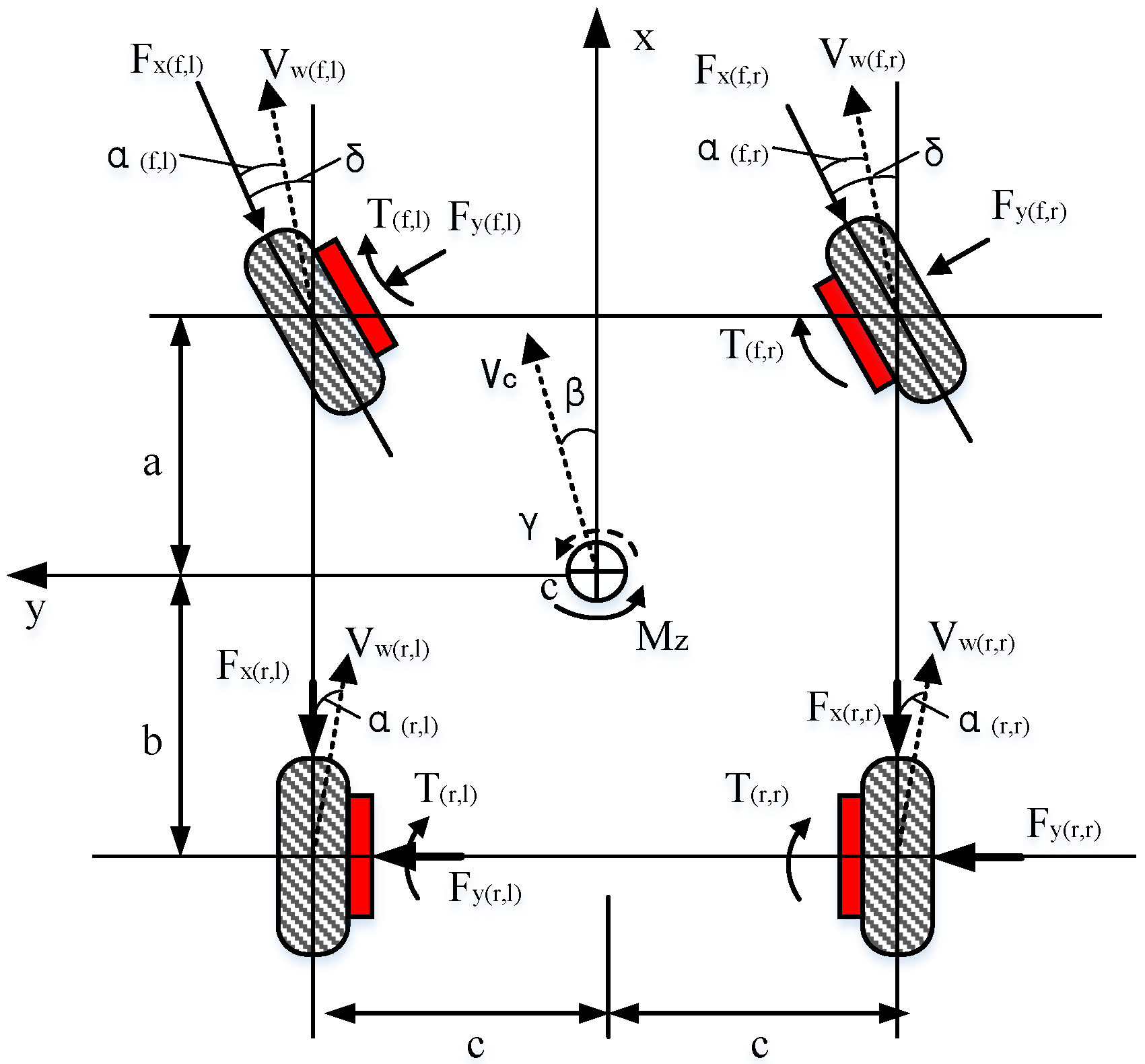
As shown in Figure 1, an FWIA EV can be simply modeled as a rigid body with three degrees of freedom. Here, only planar motions are considered for model simplification. The vehicle planar motion model contains three system states: the longitudinal velocity, the lateral velocity and the yaw rate. The equations of motion can be formulated as:
where m, Vx, Vy, ωz, Iz are the vehicle mass, longitudinal velocity, lateral velocity, yaw rate and moment inertia, respectively. Fx, Fy, Mz, Fw and Ff represent the longitudinal force, lateral force, yaw moment, air resistance and rolling resistance, respectively. Fw and Ff can be calculated as:
where CD is the aerodynamic resistance coefficient, A is the windward area, ρ is the air density, and CF is the rolling resistance coefficient.
The generalized forces and yaw moment can be expressed as:
where a is the horizontal distance between the front axle and the center of gravity (CG), b is the horizontal distance from the rear axle to CG, c is half of the track, and δf is the steering angle of the front wheels.
Ignoring the wheel vertical movement, each wheel only has one rotational freedom revolving the wheel center. The longitude force of each tire can be presented by:
where the effective radius Re and the rotational inertia Jω of tires are assumed to be the same; The subscript I = {fl, fr, rl, rr} represent different in-wheel motors, respectively, Tdi and Tbi represent the drive and brake force of each wheel, respectively.
2.2. Tire Model
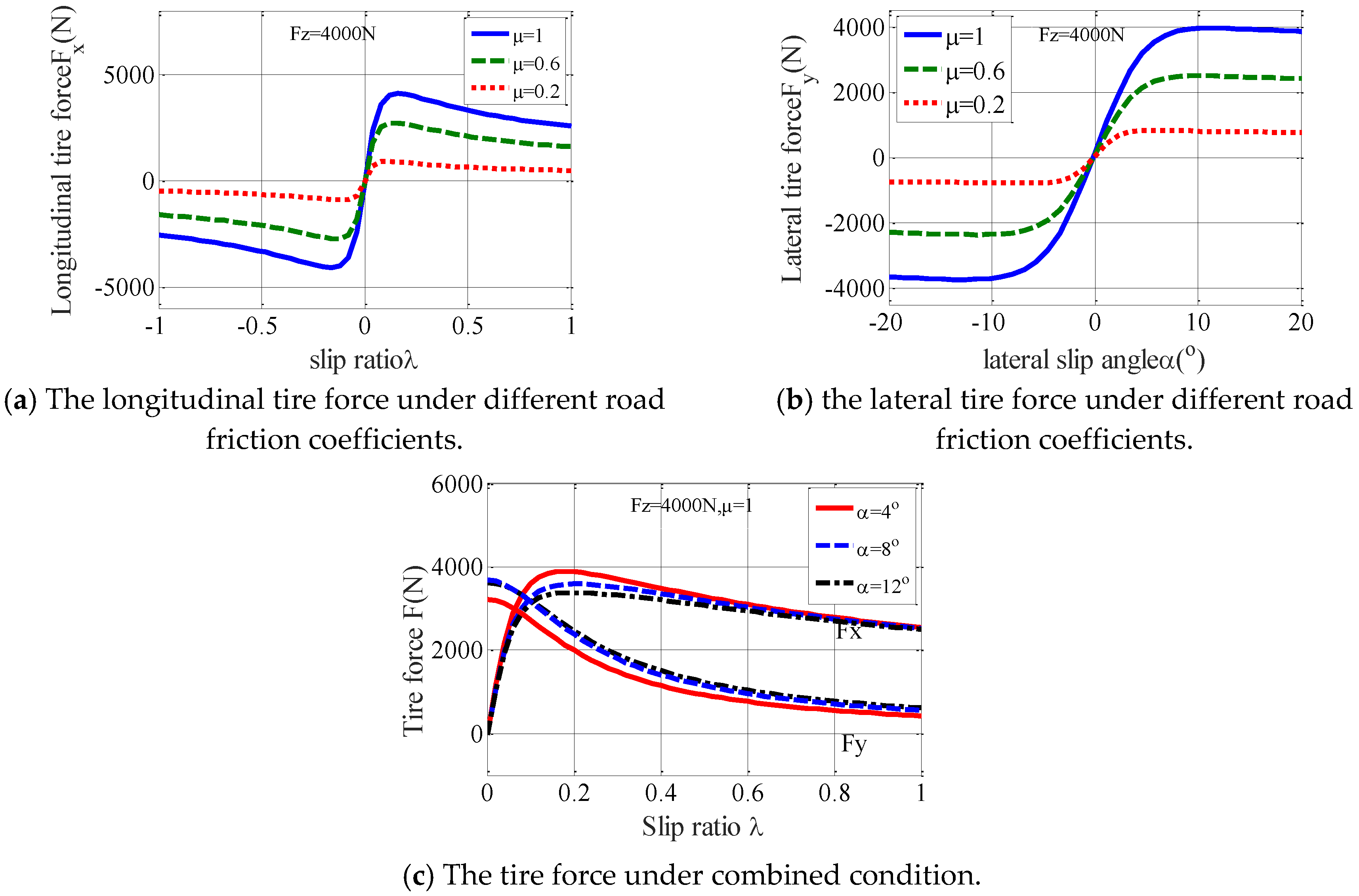
The tire model plays a critical role in the vehicle dynamics stability control. Especially, the nonlinear characteristics of tires have significant influence on the driving stability under high-speed driving conditions. The tire dynamics is usually modeled with the “Magic Formula” model developed by Pacejka [27], which is also adopted in this study. In the pure slip condition, the longitudinal force Fx is described as a nonlinear function of the vertical load Fz and the longitudinal slip ratio λ, with the lateral force Fy described as a function of the vertical load Fz and the lateral slip angle α. The basic magic formula can be expressed as:
2.3. In-Wheel Motor Model
The used in-wheel motors are permanent magnet synchronous motors (PMSMs), which are often modeled using the space vector control method. In general, the dynamic response of the PMSM torque output is much faster than the vehicle dynamics response. Thereby, the dynamic response of the motor torque can be simplified as a second-order system. The torque transfer function can be formulated as:
where ξ is the damping ratio and its value is set 0.01.
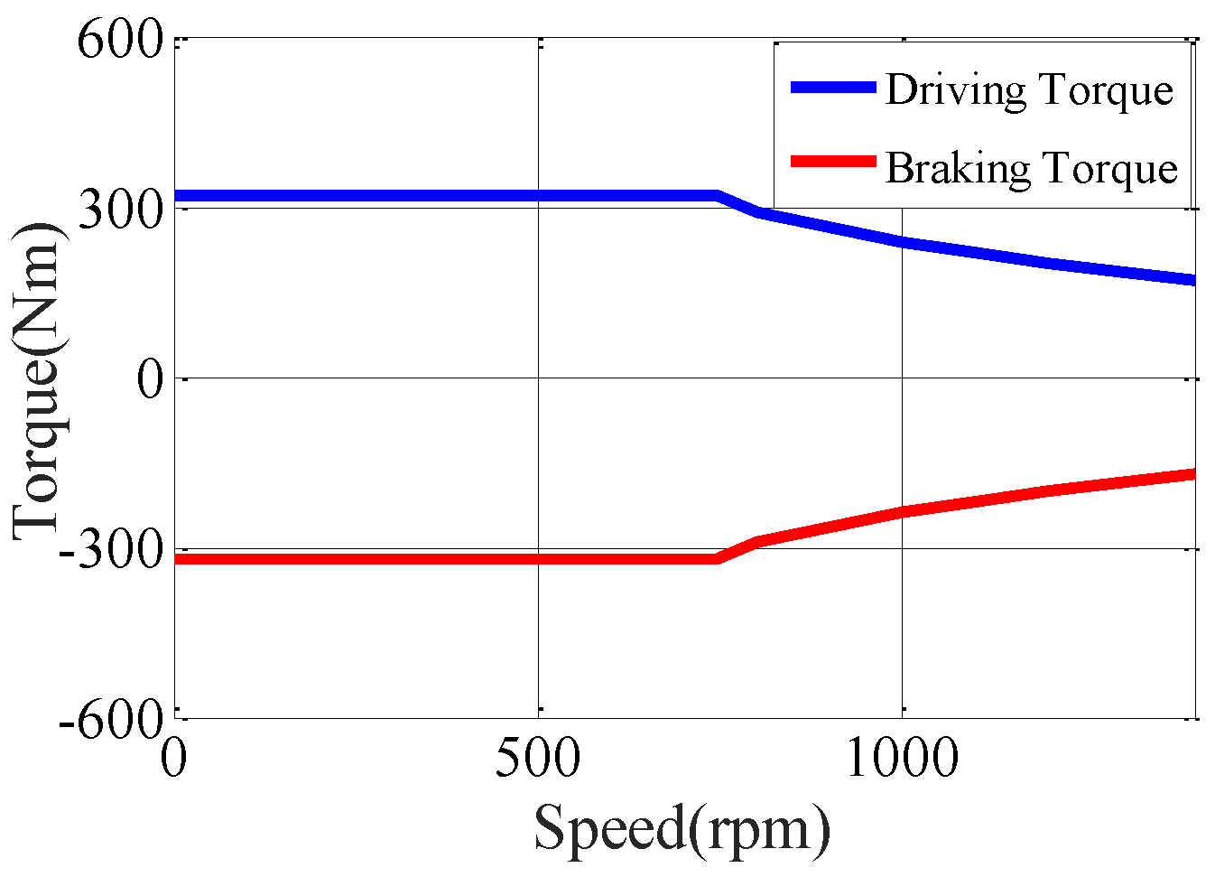
In order to meet the vehicle performance requirements, the motor is selected with a peak torque of 320 Nm and a peak power of 25 kW. The driving/braking torque limitation for each in-wheel motor is shown in Figure 3.
2.4. Driver Model
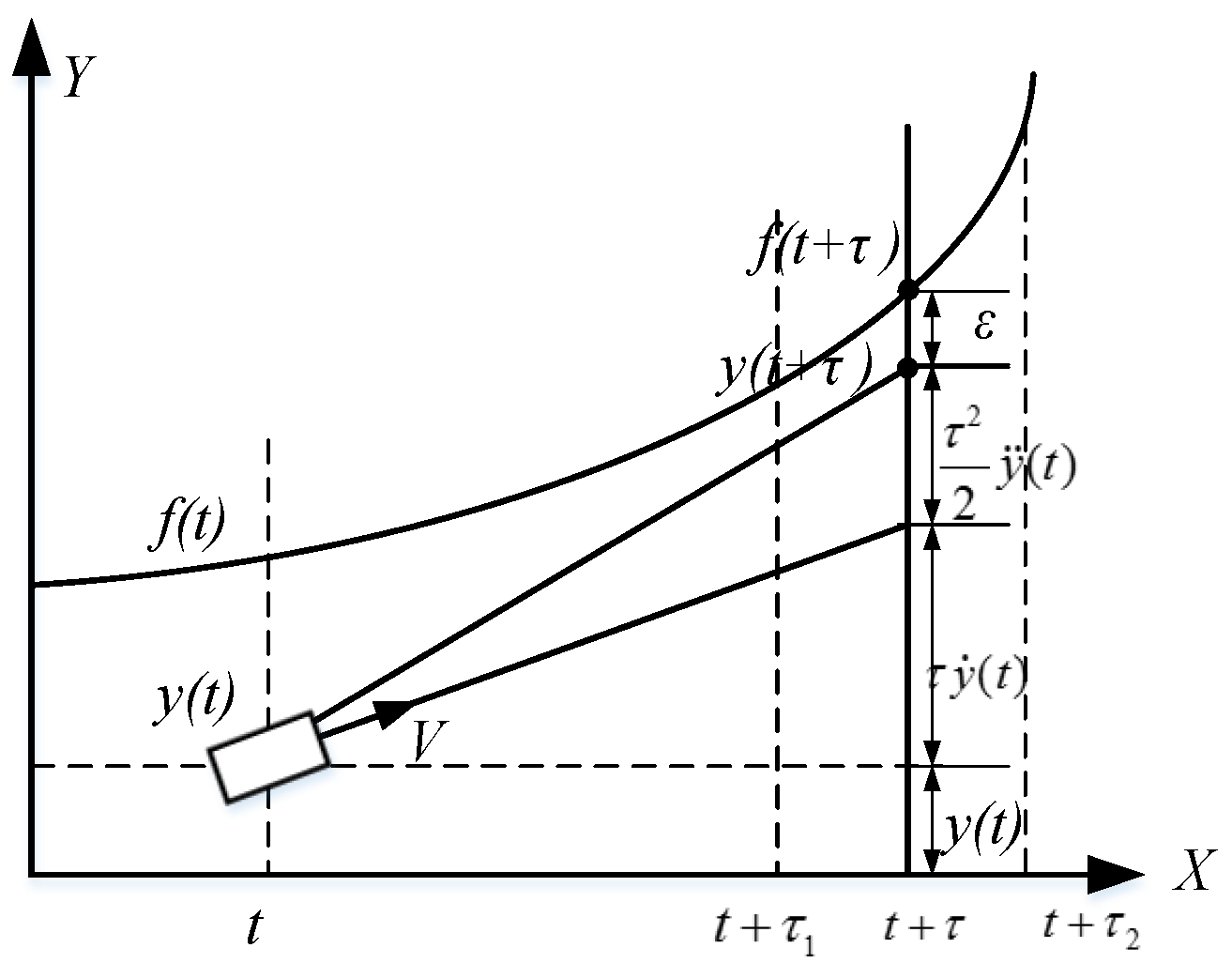
In order to achieve the trajectory tracking, a driver model based on “Preview-Follower method” developed by Guo et al. is adopted here [28]. The coordinates definition and the locating algorithm of the road tracking method are shown in the Figure 4.
Human drivers preview a distance ahead with time τ1~τ2 at the preview moment τ ∈ [τ1, τ2]. The lateral position error between the vehicle trajectory y = (t + τ) and the centerline of the desired path f(t + τ) is ε. The vehicle has the optimal steering performance by minimizing the objective function defined as:
where ω(τ) is the preview weight coefficient.
In order to ensure the vehicle run at the desired speed, a target vehicle speed tracking model is established based on the PI controller. The model outputs the accelerator pedal signal by minimizing the deviation between the actual vehicle speed and the target vehicle speed [29].
3. Vehicle Dynamics Stability Control Algorithm
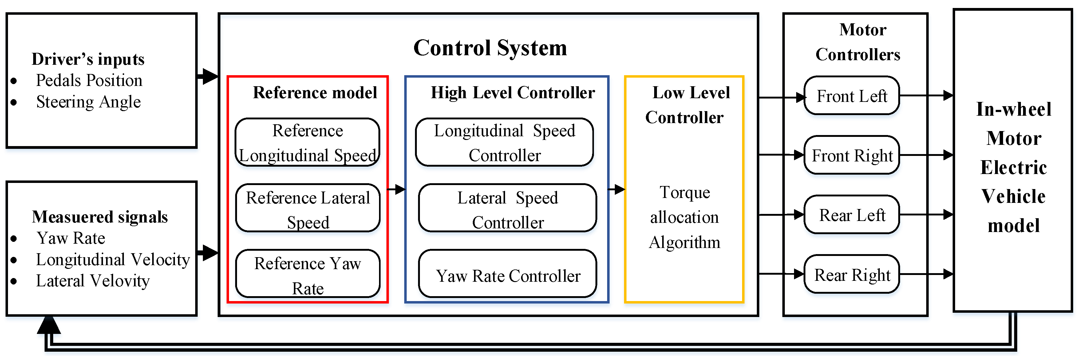
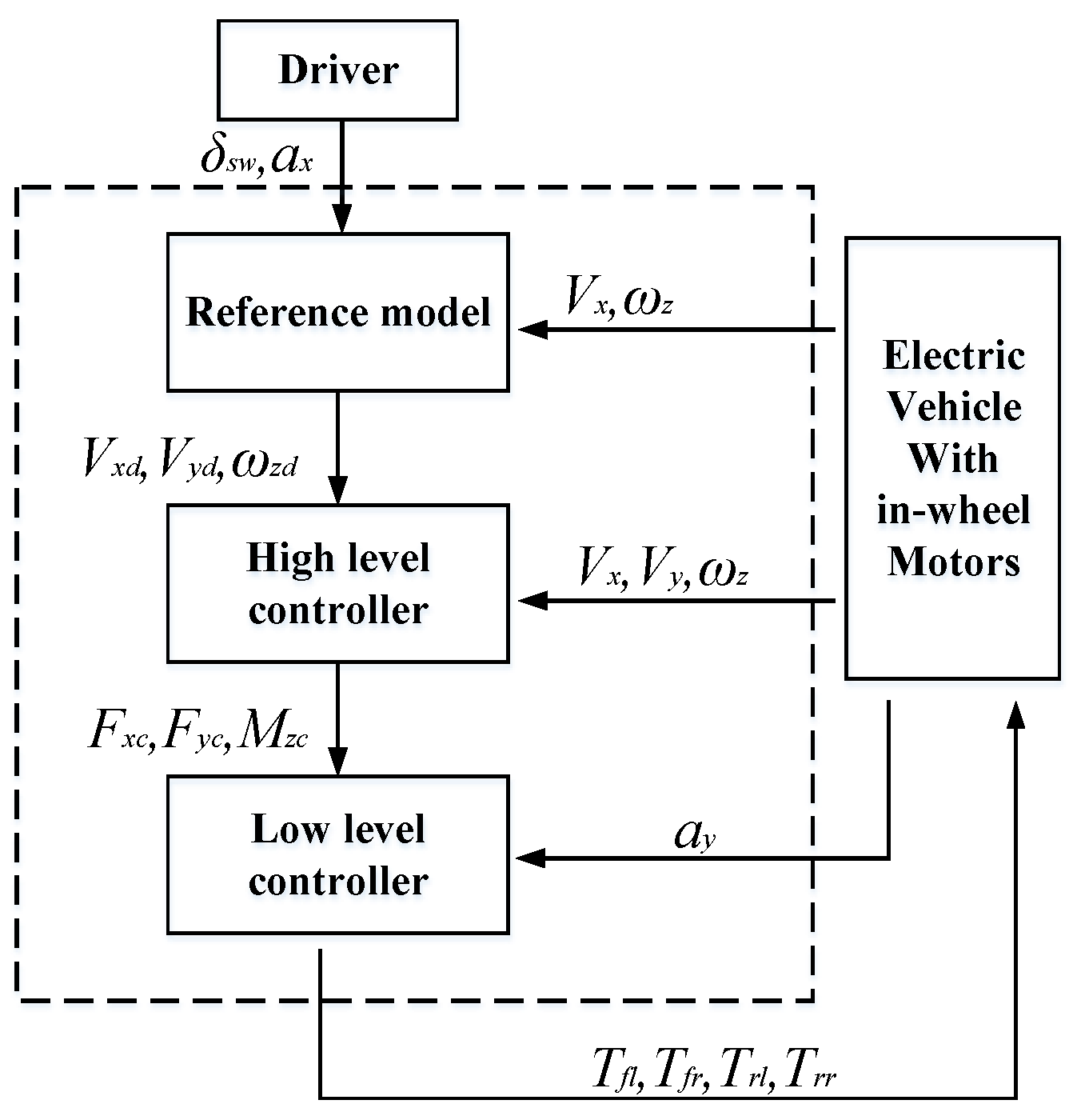
As shown in Figure 5, the flow diagram of the proposed control strategy contains a reference model and an upper and a lower controller. A reference model is designed to calculate the desired input commands, i.e., Vxd, Vyd, and ωzd, based on the driver’s instructions and the measured vehicle state information. The upper controller is designed to compute the longitudinal force Fxc, the lateral force Fyc and the yaw moment Mzc to track the desired dynamics based on the sliding mode control with a novel sliding surface design. It proves to be more robust and faster than the classic SMCs, and has better chattering phenomenon in steady state conditions. By minimizing a cost function, the lower controller is designed to obtain the driving/braking torques for each wheel. The control block diagram of the proposed controller is shown in Figure 6.
3.1. Reference Model
The reference model is used to generate the desired vehicle states and their derivatives using the driver’s inputs, the hand wheel angle, the brake pedal force, and the vehicle speed. The desired values Vxd, Vyd, ωd are derived as follows. Firstly, Vxd is computed from the pedal’s signal, assuming that the acceleration and pedal angular displacement are in an ideal linear relationship.
where V0 is the initial vehicle longitudinal velocity at time t0, and ax is the desired longitudinal acceleration/deceleration.
If the vehicle speed is constant and the lateral acceleration is limited to 0.4 g or less, the tire side characteristic is in the linear zone. According to the linear 2-degree-of-freedom model, the yaw rate of the vehicle under steady-state steering can be derived by:
where L is the wheelbase and K is:
where Cf is the front tire cornering stiffness and Cr is the rear tire cornering stiffness.
The lateral acceleration during vehicle steering is limited by the ability of tires to be attached to the road surface, and cannot exceed the lateral acceleration limit that can be provided by the road. Therefore, the upper limit of the yaw rate is:
From Equations (15) and (17), the desired yaw rate γd can be expressed as:
The desired lateral velocity Vyd is determined by:
Relationship between the yaw rate and the lateral velocity holds for the steady-state conditions derived from a linear bicycle model. It does not reflect different transient dynamics in the lateral velocity response versus yaw response in highly dynamic maneuvers, but it constitutes a sufficiently accurate approximation for the control algorithm used in this study [30].
3.2. Upper Layer Controller
The upper layer controller consists of a longitudinal velocity controller, a lateral velocity controller and a yaw stability controller. The driver’s steering angle and measurement signals of the vehicle are selected as the inputs, while the outputs include the longitudinal force Fxc, the lateral force Fyx and the yaw moment Mzc.
SMC can overcome the system uncertainties, and has strong robustness to the system disturbance and unmolded dynamics. It is a kind of control method that has good control effects on nonlinear systems. The biggest problem with sliding mode controllers is that the control output exhibits chattering effects. The method of reducing chattering mainly includes two methods: one method uses the reaching law, and the other relies on the linearization of the switching characteristic of the control inputs.
In this study, the upper layer controller is designed based on a new sliding mode control with the integral surface. The proposed SMC method is more robust and faster than classic SMCs and has lower chattering under steady state conditions [19]. The main benefits of the proposed SMC over other forms of sliding mode are that [31]: (i) it starts immediately with the sliding motion, without the requirement of the reaching phase during which the system dynamics are not the ideal ones; (ii) it can guarantee a smooth control action, without losing its properties, through the first-order filtering of the discontinuous part of its control actions.
3.2.1. Longitudinal Velocity Controller
The longitudinal velocity controller is to compute the desired longitudinal force Fxc for maintaining the desired longitudinal velocity Vx. The sliding surface is defined as:
The reaching law is synthesized as:
According to Equation (1), the longitudinal velocity control law can be designed as:
where c1 > 0, η1 > 0, and Fr = Fw + Ff.
3.2.2. Lateral Speed Controller
The lateral speed controller is designed to calculate the desired longitudinal force Fyx, in order to track the desired lateral speed Vyd and enhance the lateral stability. The sliding surface is defined as follows:
The reaching laws is:
Based on Equation (2), the lateral velocity control law is designed as follows:
where c2 > 0, η2 >0.
3.2.3. Yaw Rate Controller
In order to enhance the lateral stability and track the desired yaw rate ωzd, a yaw rate controller is designed to generate the desired yaw moment Mzc. The sliding surfaces is defined as:
The reaching law is:
According to Equation (3), the yaw rate control law can be deduced as:
where c3 > 0, η3 > 0.
3.3. Lower Layer Controller
The torque distribution algorithm is needed to obtain the motor drive/brake torque at each wheel to provide the desired vehicle yaw moment that help track the desired value of the traction force and the yaw moment determined by the upper layer controller. Two different torque distribution methods, namely, dynamic-load-based and optimization-based strategies are described and compared in the following parts.
3.3.1. Dynamic-Load-Based Control
The vertical load on each wheel is not equal all the time during vehicular operations, especially during the steering process, due to the existence of longitudinal and lateral accelerations. In addition, the maximum adhesion force of each wheel is related to the road friction coefficient and the wheel vertical load. The maximum adhesion force will increase with the enlarging wheel vertical load when the road friction coefficient is assumed to be constant. Therefore, the influence of the wheel vertical load on the electronic stability should be taken into account in the torque distribution algorithm. That is, the traction torque distributed to the wheel with the greater adhesion ability should be higher, and vice versa. In this case, the adhesion force of each wheel can be used more effectively, which prevents wheels slippery and thus enhances the vehicle dynamics stability. [21] The dynamic-load-based torque distribution strategy is used to distribute the traction torque and the yaw moment considering the change of each wheel’s vertical load, which can be described as Equation (29). The dynamic load distribution ratio ζi (i = fl, fr, rl and rr) is given by Equation (30).
where Fzi (i = fl, fr, rl, and rr) is the vertical load of the ith wheel, which can be calculated using the longitudinal acceleration ax and the lateral acceleration ay obtained from the vehicle model in CarMaker. Fz = Fzfl + Fzfr + Fzrl + Fzrr is the total vertical load of the four wheels, ζi (i = fl, fr, rl, and rr) is the distribution ratio of the left front wheel, the right front wheel, the left rear wheel, and the right rear wheel, respectively. The in-wheel motor torque inputs based on the dynamic-load-based torque distribution strategy can be expressed as:
where ΔM is the deviation between Mzc and Mz.
3.3.2. Optimization-Based Control
The generated tire force/moment by the upper layer controller is defined as Fv, with the coefficient matrix as Bv and the input as u. Then, according to Equations (6)–(8), (22), (25) and (28), the matrix can be defined as:
In order to achieve precise handling and vehicle dynamics stability control of the FWIA EV, an objective function based on the constrained tracking problem is designed.
(1) The main control target is to ensure good handling stability under different conditions, while making the vehicle Vx, Vy and ωz track the reference Vxd, Vyd and ωzd with high accuracy. Optimum torque allocation control is used to convert virtual control information to physical control inputs for available sets of motors. The cost function is defined as:
where Wv is positive weight factors for adjusting tracking performance, and the weight matrix is defined as Wv = diag(Wv1, Wv2, Wv3).
(2) Since the tire workload usage has an important influence on the vehicle dynamics stability, the objective function is then formulated as:
where Ci (i = fl, fr, rl, and rr) is the tire longitudinal force weight factor.
The constraint conditions are shown as follows:
(1) Ti should meet output/input capability requirements of in-wheel motors.
where Tdmax and Tbmax represent the maximum driving and braking torques of in-wheel motors, respectively.
(2) To ensure the handling stability of the vehicle, the tire longitudinal and lateral forces need to meet the friction ellipse constraints, which can be formulated as:
Therefore, the total objective function of the optimal control problem can be defined as:
The optimal control problem can be solved by the Sequential Quadratic Programming (SQP), which is widely used for its ability to deal with inequality constraints and global and super-linear convergence.
4. Simulation and Experimental Results
In order to verify the effectiveness of the proposed control strategy, co-simulation based on the software of Matlab/Simulink and CarMaker and hardware-in-loop (HIL) experiments were both carried out in a closed-loop system including vehicle, driver and road. Control allocation strategies based on the tire-dynamic-load and optimization are verified under double lane change maneuver with different friction coefficients.
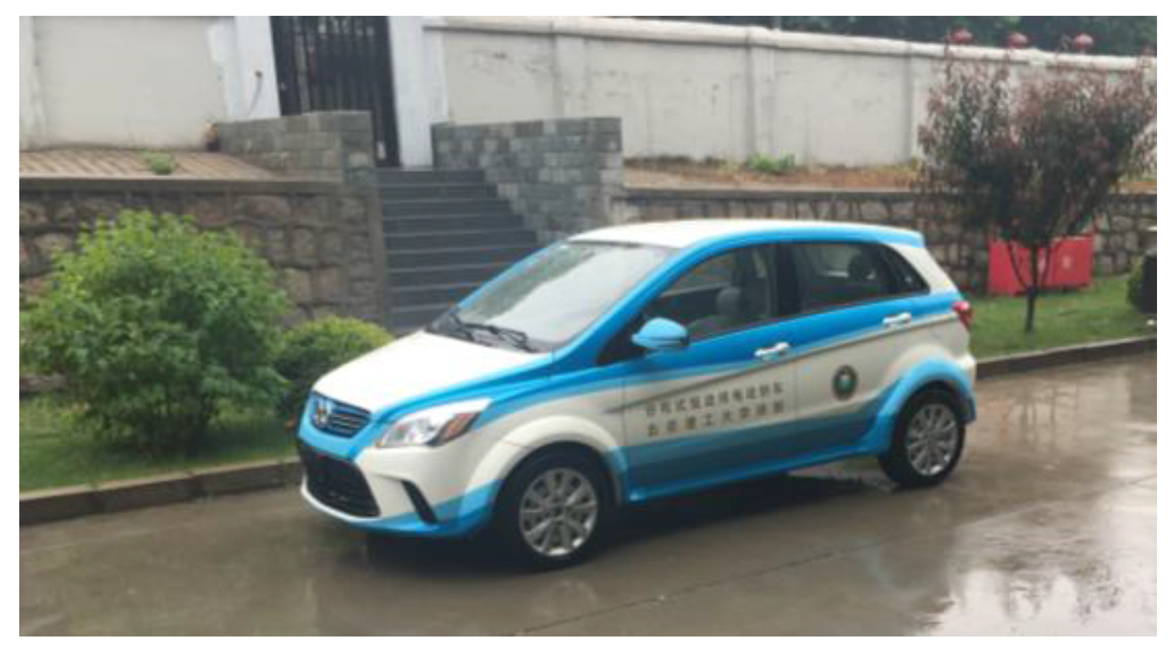
An experimental prototype has been developed in our lab based on the EV160 model manufactured by Beijing Electric Vehicle Co., Ltd., Beijing, China, as shown in Figure 7. Its main parameters are listed in detail in Table 1. It is worth mentioned that the model parameters used in this study are obtained on the basis of this prototype. And several preliminary tests have been conducted to assure the parameter consistency between the simulation model and the real experimental prototype.
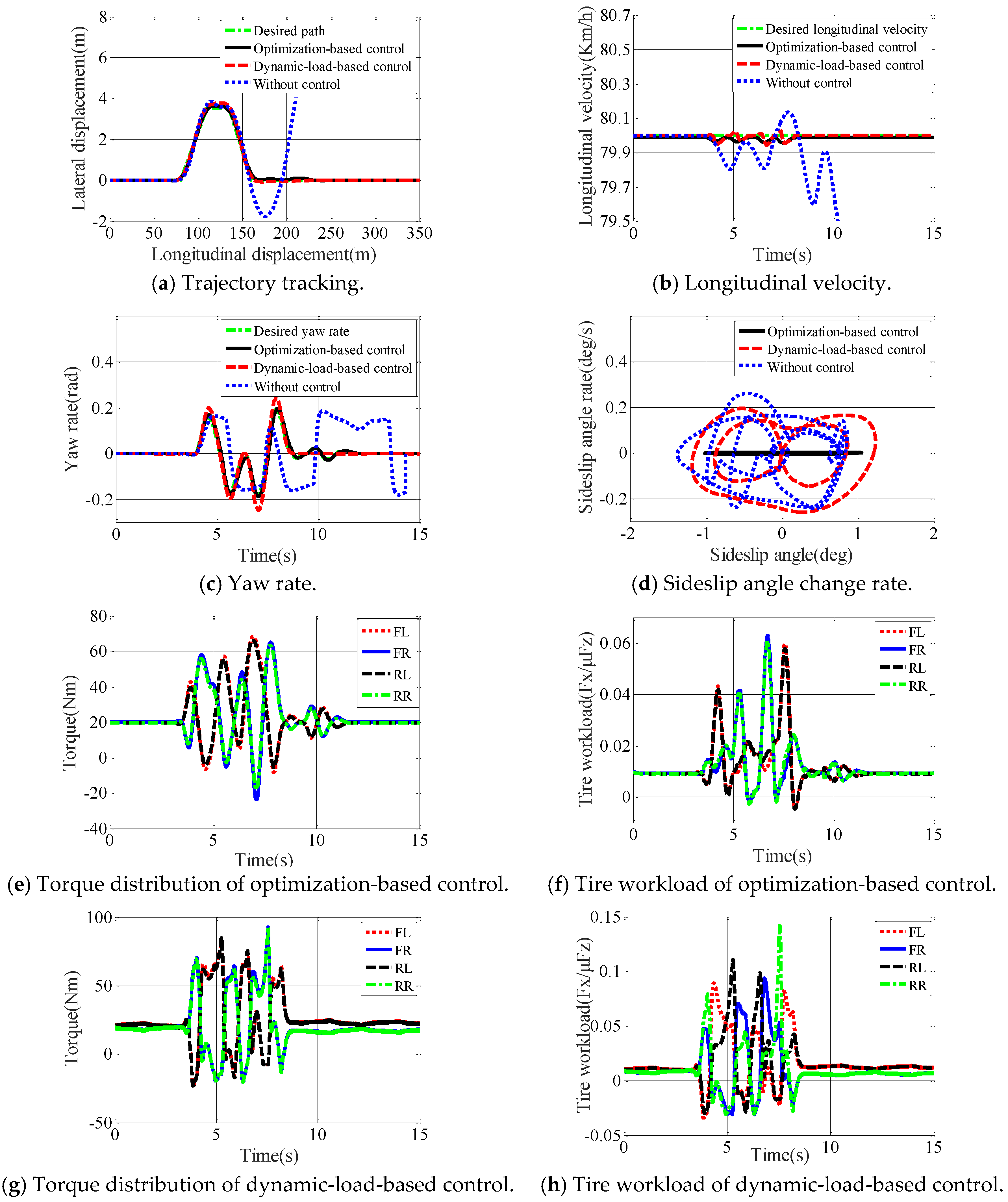
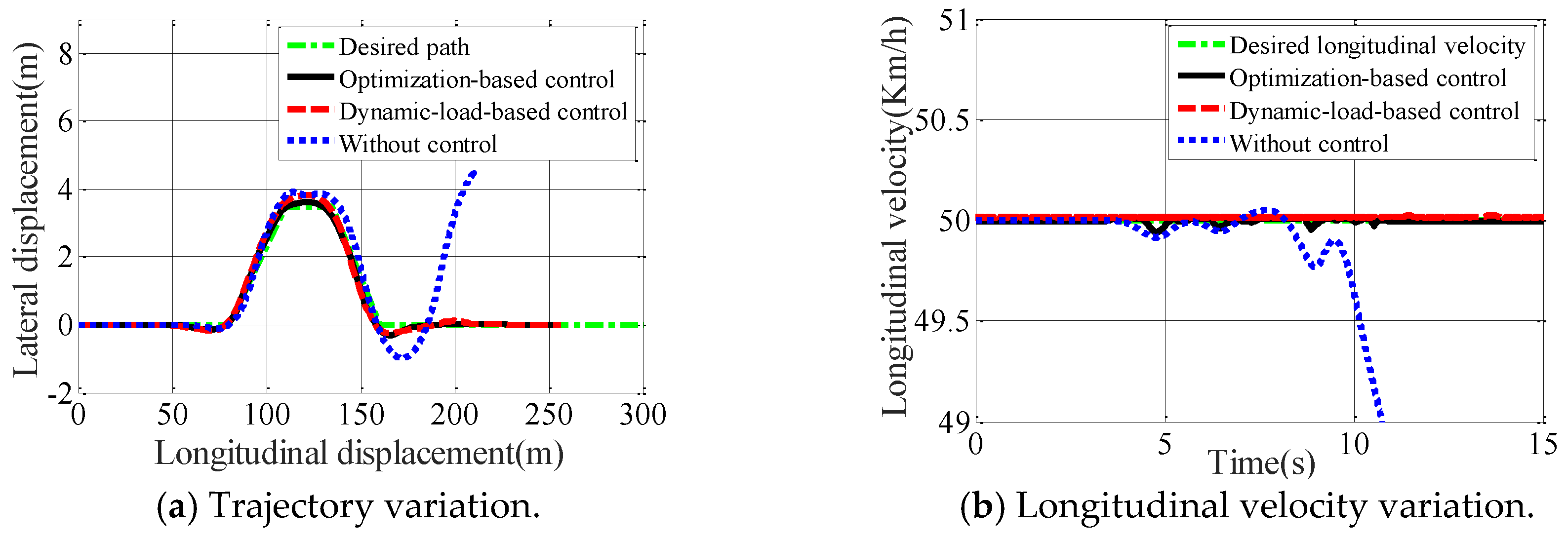
4.1. Double Lane Change Maneuver with High Frictions
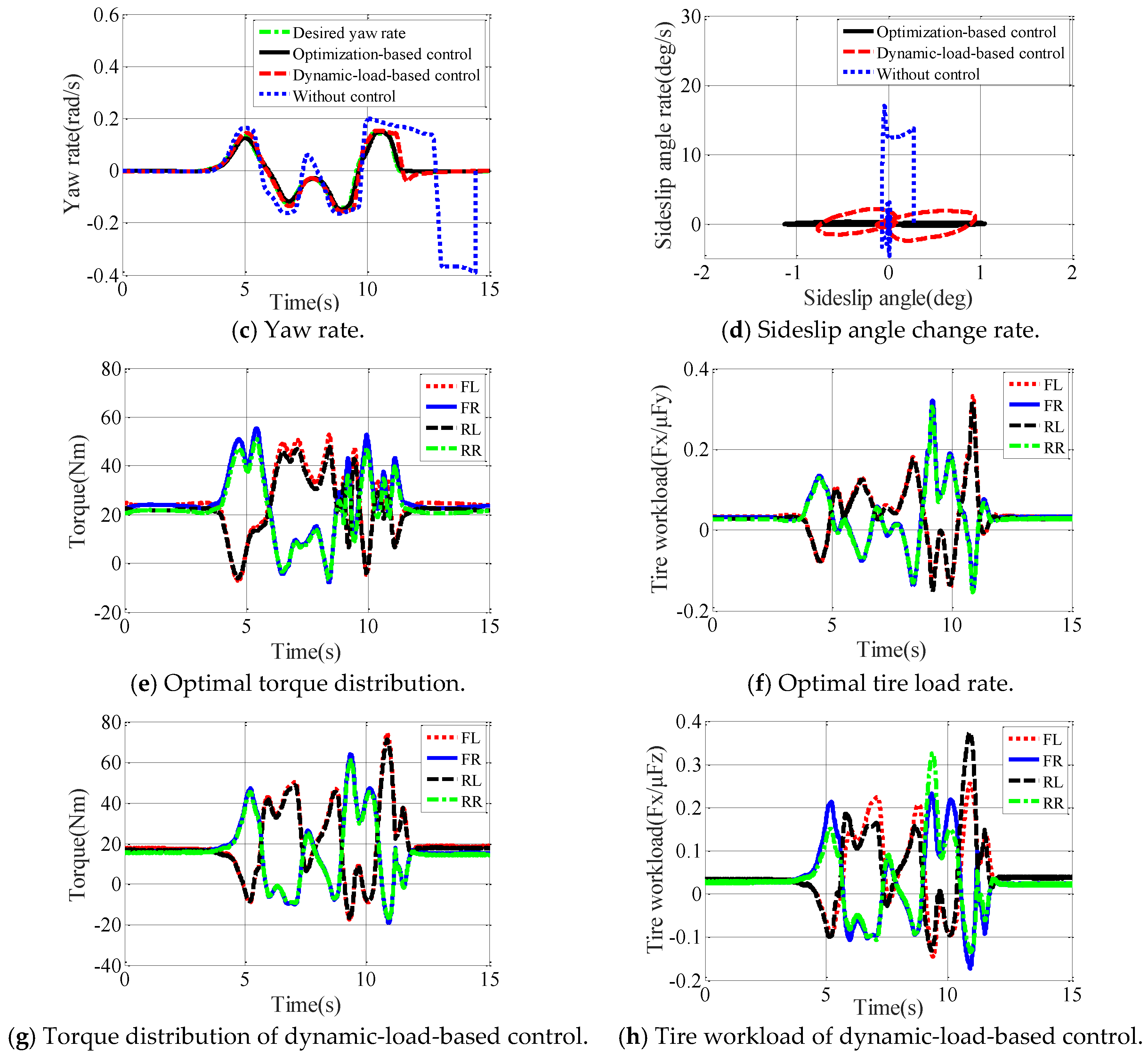
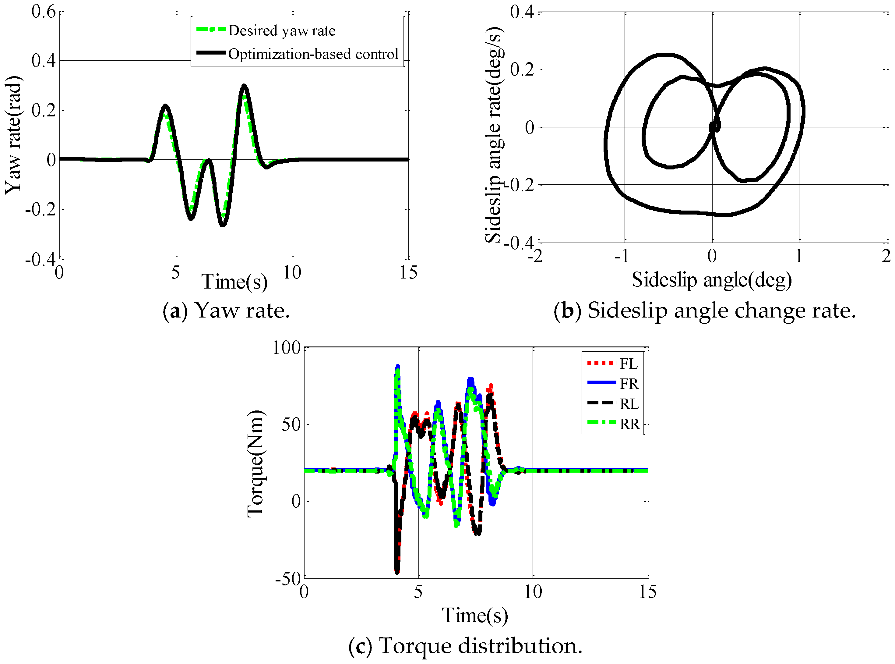
Road adhesion coefficient is set as μ = 1 with a target speed of 80 km/h. From a close observation of Figure 8a, it can be seen that both the dynamic-load-based control and optimization-based control can make the vehicle closely track the preset trajectory. However, the optimization-based control yields better performance than the dynamic-load-based control scheme. Figure 8b presents a comparison of the velocity retention capability of the two control schemes under the double lane change maneuver. It is obvious that the optimization-based control and the dynamic-load-based control can maintain the vehicle speed throughout the test regime, while the vehicle failed without control. Figure 8c shows that the dynamic-load-based control can follow the desired yaw rate with some deviation, while the optimization-based control can track the desired yaw rate more closely. In contrast, the vehicle without control cannot track the trajectory or the reference yaw rate.
Despite that the phase plane for the optimization-based control and the dynamic-load-based control can eventually converge, the convergence processes are different as shown in Figure 8d. The change rate of the sideslip angle for the proposed torque distribution is smallest, which indicates that the control effect is more stable. The vehicle without control exhibits obvious oscillatory response and loses the yaw motion stability.
It can be seen from Figure 8e, the torques are assigned to different wheels on both sides under the double lane change maneuver in order to ensure the vehicle lateral stability. The torque distribution trends of two wheels on the same side are similar under the proposed optimization-based control.
In understeering or oversteering situations, considering the tire load and the output ability of in-wheel motors, the additional yaw moment is realized by assigning the torque demands to different wheels, resulting in improved vehicle lateral stability and maneuverability. Compared with the rear wheels, the torques of the front wheel motors are more prone to reaching the constraint boundaries. This is because the front wheels are also used as the steering wheels that usually contribute to more lateral force and yaw moment. As seen from Figure 8f, with the proposed torque distribution strategy, the tire workload is generally small, which means that the vehicle has more ability to maintain the handling and dynamics stability.
In contrast, seen from Figure 8g and 8h, under the dynamic-load-based torque distribution strategy, the tire workload is large, and the vehicle capability to maintain the vehicle dynamics stability would be limited.
4.2. Double Lane Change Maneuver with Low Friction
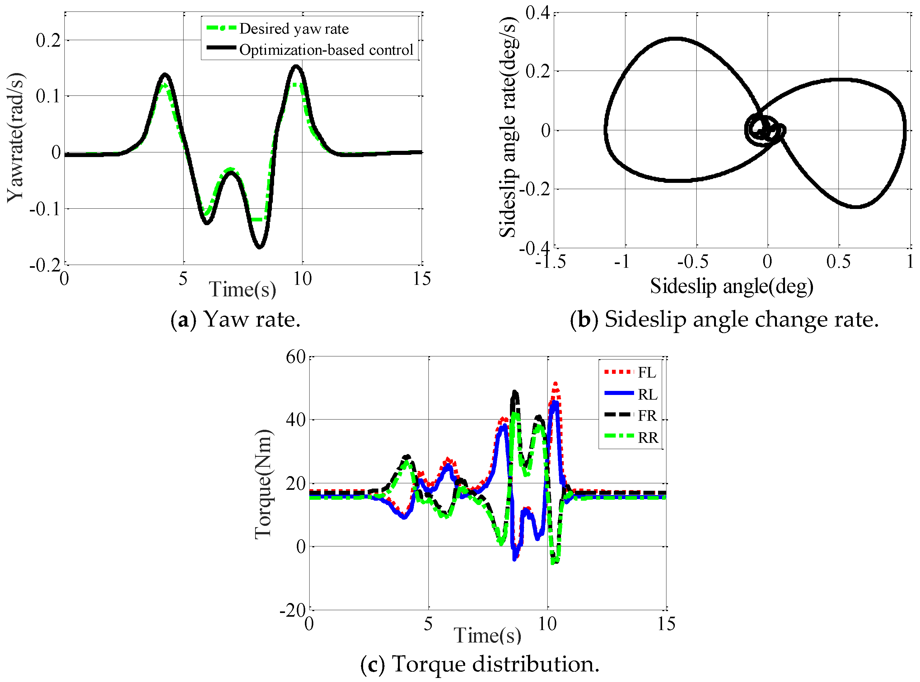
In order to further evaluate the handling and stability performance of the proposed method, the FWIA model is driven on low-friction coefficient roads under the DLC maneuver, which is specially used to evaluate the lateral dynamics stability of a vehicle. Road friction coefficient is set to be 0.2 with a target speed of 50 km/h.
As shown in Figure 9a–c, the optimal torque distribution strategy stages the best performance in tracking the trajectory, longitudinal velocity and yaw rate, with the smallest operating pressure from the driver. The dynamic-load-based control strategy comes the second. As can be seen from Figure 9d, both the optimal torque distribution strategy and the dynamic-load-based control can effectively control the sideslip angle with similar effects. From Figure 9e and Figure 8e, there is little difference in the drive torque between the two wheels at the same sides. This is because when the required yaw moment is small, the lateral force generated by the front wheels is quite limited.
As seen Figure 9f,h, the tire workloads of two control strategies are both larger than that under the high-friction adhesion coefficient condition. At the same time, due to the roll movement of the vehicle, the tire load rate of the same side wheel changes greatly when the vehicle turns.
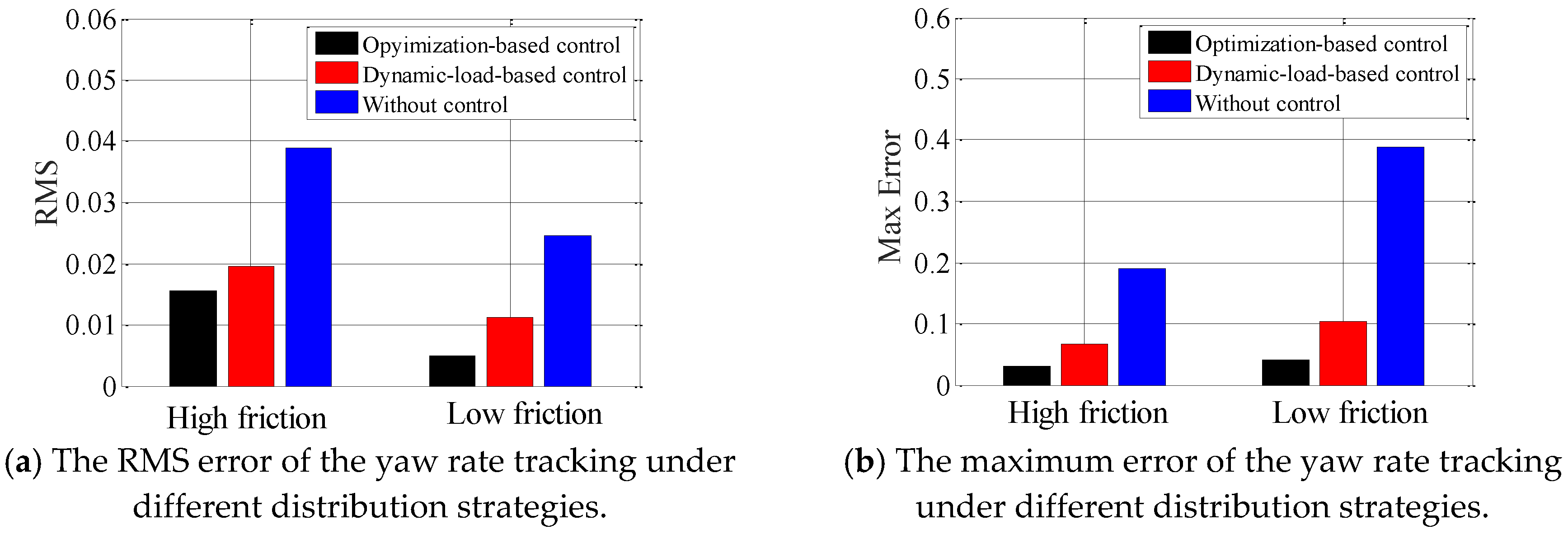
The root mean square and the maximum error of the yaw rate are used to numerically assess the performance of the different control allocation strategies under different maneuvers as shown in Figure 10.
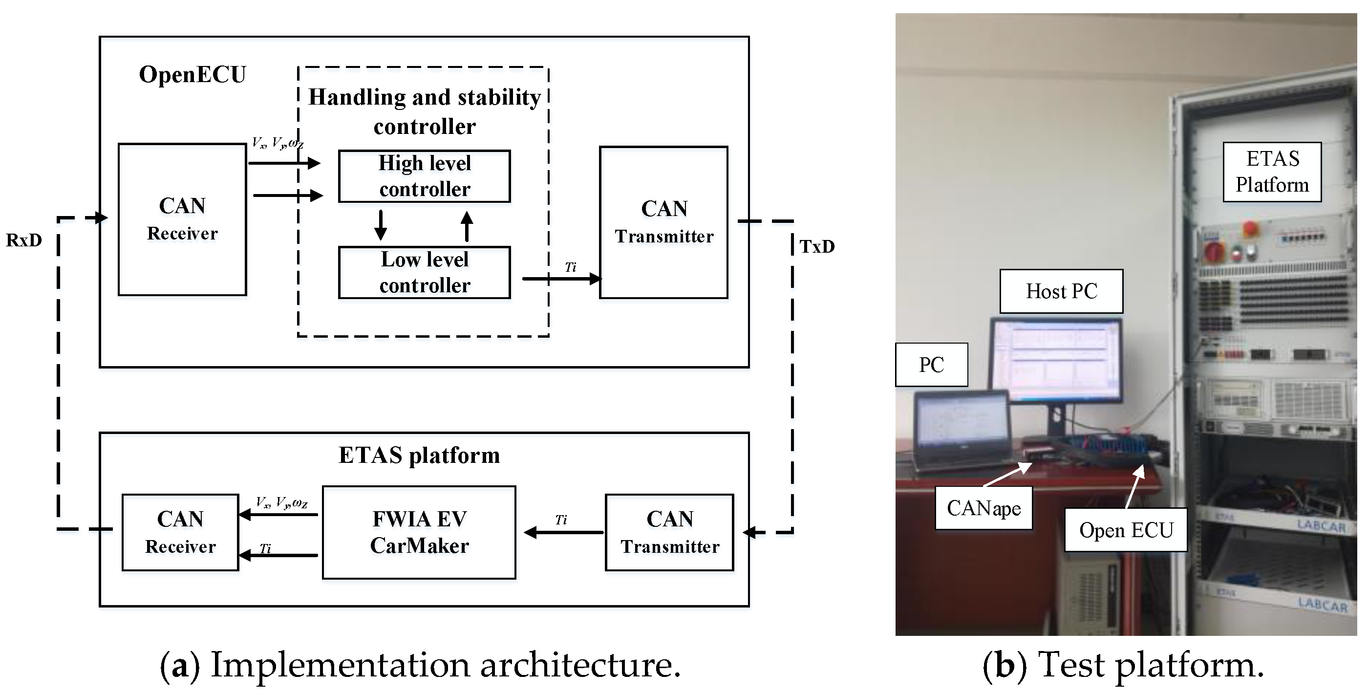
4.3. Experimental Results
A HIL platform was set up to further verity the proposed control strategy. It consists of a host computer, an Open ECU controller and the ETAS hardware. As shown in Figure 11, CarMaker is run on the real-time ETAS platform while the proposed control strategy is implemented on the Open ECU controller. The platform and the controller communicate with each other by Controller Area Network (CAN).
The real-time experiments results are shown in Figure 12 and Figure 13. It can be seen that the designed controller meets the demand of real-time control. However, compared with the simulation results shown in Section 4.1 and Section 4.2, there is a certain tracking deviation. There are several reasons. First, the controller is running based on the solver of fixed step that leads to difference from the simulation results of off-line simulation. Second, the CAN bus uses a periodic transmission mode, which results in a certain information transmit lag such as control commands and vehicle states. In addition, the quantization errors result in low measuring precision of the system output and the controller output.
5. Conclusions
This paper presents a hierarchical control strategy for a four-wheel-independently-actuated electric vehicle to improve vehicle dynamics stability and handling performance. It comprises of an upper layer and a lower layer controller. The upper layer controller employs an improved sliding mode control approach to generate the desired force/moment. The lower layer controller is responsible for achieving torque allocation for each in-wheel motor. The performance of the proposed control strategy has been examined under double lane change tests through both simulation and HIL experimental studies. The results show that the proposed SMC can effectively track the desired commands while having lower chattering effect. Particularly, in comparison to the rule-based control strategy, it exhibits superiority in ensuring vehicle dynamics stability in terms of yaw rate tracking and sideslip angle confinement. This validates the effectiveness of the proposed control strategy for FWIA EVs.
Acknowledgments
The project was supported by the Funds of Beijing Municipal Science & Technology Commission (No. B160603) and the National Key R&D Program of China (No. 2017YFB0103600).
Author Contributions
Zhenpo Wang and Yachao Wang built the vehicle dynamics model for the four-wheel-independently-actuated electric vehicle. Yachao Wang and Lei Zhang collaboratively developed the control strategy and conducted HIL experiments. Mingchun Liu helped with the simulation. All authors carried out the data analysis, discussed the results and contributed to writing the paper.
Conflicts of Interest
The authors declare no conflict of interest.
References
- Yu, Z.; Feng, Y.; Xiong, L. Review on Vehicle Dynamics Control of Distributed Drive Electric Vehicle. J. Mech. Eng. 2013, 8, 105–114. [Google Scholar] [CrossRef]
- Pasterkamp, W.R.; Pacejka, H.B. The Tyre as a Sensor to Estimate Friction. Veh. Syst. Dyn. Int. J. Veh. Mech. Mobil. 2007, 27, 409–422. [Google Scholar] [CrossRef]
- Zanten, A.; Bosch, R. Evolution of Electronic Control Systems for Improving the Vehicle Dynamic Behavior. In Proceedings of the 6th International Symposium on Advanced Vehicle Control, Yokohama, Japan, 9–13 September 2002. [Google Scholar]
- Park, K.; Heo, S.; Baek, I. Controller design for improving lateral vehicle dynamic stability. JSAE Rev. 2001, 22, 481–486. [Google Scholar] [CrossRef]
- Pennycott, A.; Novellis, L.; Gruber, P.; Sorniotti, A.; Goggia, T. Enhancing the Energy Efficiency of Fully Electric Vehicles via the Minimization of Motor Power Losses. In Proceedings of the 2013 IEEE International Conference on Systems, Man, and Cybernetics (SMC), Manchester, UK, 3–16 October 2013; pp. 4167–4172. [Google Scholar]
- Nam, K.; Fujimoto, H.; Hori, Y. Lateral Stability Control of In-Wheel-Motor-Driven Electric Vehicles Based on Sideslip Angle Estimation Using Lateral Tire Force Sensors. IEEE Trans. Veh. Technol. 2012, 61, 1972–1985. [Google Scholar]
- Jonasson, M.; Andreasson, J.; Solyom, S.; Jacobson, B.; Trigell, A. Utilization of Actuators to Improve Vehicle Stability at the Limit: From Hydraulic Brakes Toward Electric Propulsion. J. Dyn. Syst. Meas. Control 2011, 133, 502–506. [Google Scholar] [CrossRef]
- Doumiati, M.; Victorino, A.; Charara, A.; Lechner, D. Onboard Real-Time Estimation of Vehicle Lateral Tire—Road Forces and Sideslip Angle. IEEE/ASME Trans. Mech. 2011, 16, 601–614. [Google Scholar] [CrossRef]
- Gordon, T.; Howell, M.; Brandao, F. Integrated control methodologies for road vehicles. Veh. Syst. Dyn. 2003, 40, 157–190. [Google Scholar] [CrossRef]
- Doumiati, M.; Sename, O.; Dugard, L.; Martinez-Molina, J.-J.; Gaspar, P.; Szabo, Z. Integrated vehicle dynamics control via coordination of active front steering and rear braking. Eur. J. Control 2013, 19, 121–143. [Google Scholar] [CrossRef]
- Yin, D.; Shan, D.; Chen, B. A torque distribution approach to electronic stability control for in-wheel motor electric vehicles. In Proceedings of the 2016 IEEE International Conference on Applied System Innovation (ICASI 2016), Okinawa, Japan, 26–30 May 2016. [Google Scholar]
- Wang, J.; Longoria, R. Coordinated and reconfigurable vehicle dynamics control. IEEE Trans. Control Syst. Technol. 2009, 17, 723–732. [Google Scholar] [CrossRef]
- Johansen, T.; Fossen, T. Control allocation—A survey. Automatica 2013, 49, 1087–1103. [Google Scholar] [CrossRef]
- Chong, F.; Ding, N.; He, Y.; Xu, G.; Gao, F. Control allocation algorithm for over-actuated electric vehicles. J. Cent. South Univ. 2014, 21, 3705–3712. [Google Scholar]
- Liu, M.; Zhang, C. Development of an optimal control system for longitudinal and lateral stability of an individual eight-wheel-drive electric vehicle. Int. J. Veh. Des. 2015, 69, 132–150. [Google Scholar] [CrossRef]
- Yu, Z.; Leng, B.; Xiong, L.; Feng, Y.; Shi, F. Direct yaw moment control for distributed drive electric vehicle handling performance improvement. Chin. J. Mech. Eng. 2016, 29, 486–497. [Google Scholar] [CrossRef]
- Xiong, L.; Teng, W.; Yu, Z.; Zhang, W.; Feng, Y. Novel stability control strategy for distributed drive electric vehicle based on driver operation intention. Int. J. Autom. Technol. 2016, 17, 651–663. [Google Scholar] [CrossRef]
- Zhao, H.; Gao, B.; Ren, B.; Deng, W. Model predictive control allocation for stability improvement of four-wheel drive electric vehicles in critical driving condition. IET Control Theory Appl. 2015, 19, 2688–2696. [Google Scholar] [CrossRef]
- Alipour, H.; Sabahi, M.; Sharifian, M. Lateral stabilization of a four wheel independent drive electric vehicle on slippery roads. Mechatronics 2015, 30, 275–285. [Google Scholar] [CrossRef]
- Li, B.; Du, H.; Li, W. Optimal Distribution Control of Non-Linear Tire Force of Electric Vehicles with In-Wheel Motors. Asian J. Control 2016, 18, 69–88. [Google Scholar] [CrossRef]
- Zhai, L.; Sun, T.; Wang, J. Electronic Stability Control Based on Motor Driving and Braking Torque Distribution for a Four In-Wheel Motor Drive Electric Vehicle. IEEE Trans. Veh. Technol. 2016, 65, 4726–4739. [Google Scholar] [CrossRef]
- Wang, J.; Wang, R.; Jing, H.; Chen, N. Coordinated Active Steering and Four-wheel Independently Driving/Braking Control with Control Allocation. In Proceedings of the 2015 American Control Conference, Chicago, IL, USA, 1–3 July 2015. [Google Scholar]
- Le, A.; Chen, C. Vehicle stability control by using an adaptive sliding-mode algorithm. Int. J. Veh. Des. 2016, 72, 107–131. [Google Scholar] [CrossRef]
- Wang, Q.; Ayalew, B.; Singh, A. Control Allocation for Multi-Axle Hub Motor Driven Land Vehicles. SAE Int. J. Altern. Powertrains 2016, 5, 338–347. [Google Scholar] [CrossRef]
- Polesel, M.; Shyrokau, B.; Tanelli, M.; Savitski, D.; Ivanov, V.; Ferrara, A. Hierarchical control of overactuated vehicles via sliding mode techniques. In Proceedings of the 53rd IEEE Conference on Decision and Control, Los Angeles, CA, USA, 15–17 December 2014. [Google Scholar]
- Canale, M.; Fagiano, L.; Ferrara, A.; Vecchio, C. Vehicle Yaw Control via Second-Order Sliding-Mode Technique. IEEE Trans. Ind. Electron. 2008, 55, 3908–3916. [Google Scholar] [CrossRef]
- Kuiper, E.; Van Oosten, J.J.M. The PAC2002 advanced handling tire model. Veh. Syst. Dyn. 2007, 45, 153–167. [Google Scholar] [CrossRef]
- Guo, K.; Peng, F. Preview optimized artificial neural network driver model. Chin. J. Mech. Eng. 2003, 39, 26–29. [Google Scholar] [CrossRef]
- Fallah, S.; Khajepour, A.; Fidan, B.; Chen, S.-K.; Litkouhi, B. Vehicle Optimal Torque Vectoring Using State-Derivative Feedback and Linear Matrix Inequality. IEEE Trans. Veh. Technol. 2013, 62, 1540–1552. [Google Scholar] [CrossRef]
- Hac, A.; Doman, D.; Oppenheimer, M. Unified Control of Brake- and Steer-by-Wire Systems Using Optimal Control Allocation Methods. In Proceedings of the 2006 SAE World Congress, Detroit, MI, USA, 3 April 2006. [Google Scholar]
- Goggia, T.; Sorniotti, A.; De Novellis, L.; Ferrara, A.; Gruber, P.; Theunissen, J.; Steenbeke, D.; Knauder, B.; Zehetner, J. Integral Sliding Mode for the Torque-Vectoring Control of Fully Electric Vehicles: Theoretical Design and Experimental Assessment. IEEE Trans. Veh. Technol. 2015, 64, 1701–1715. [Google Scholar] [CrossRef]
Figure 1.
Coordinates for planar motions.

Figure 2.
The tire force under different conditions.

Figure 3.
Driving torque and regenerative torque characteristics of in-wheel motor.

Figure 4.
Human diver model.

Figure 5.
Process flow diagram of the driving control algorithm.

Figure 6.
The control block diagram of the proposed controller.

Figure 7.
The experimental prototype.

Figure 8.
Simulation results for double lane change with high friction.

Figure 9.
Simulation results for double lane change with low friction.


Figure 10.
Simulation results for double lane change with low friction.

Figure 11.
Hardware in the loop.

Figure 12.
Experimental results for double lane change with high friction.

Figure 13.
Experimental results for double lane change with low friction.


Table 1.
The main parameters of the prototype.
| Variable Parameters | Notation | Value | Unit |
|---|---|---|---|
| Vehicle mass | m | 1600 | kg |
| Moment of inertia around Z axis | Iz | 1975 | kg·m2 |
| Distance from center of mass to front axle | a | 1.085 | m |
| Distance from center of mass to rear axle | b | 1.386 | m |
| Centroid height | H | 0.48 | m |
| Wheel-track | B | 1.429 | m |
| Wheel effective radius | R | 0.281 | m |
© 2017 by the authors. Licensee MDPI, Basel, Switzerland. This article is an open access article distributed under the terms and conditions of the Creative Commons Attribution (CC BY) license (http://creativecommons.org/licenses/by/4.0/).
Share and Cite
MDPI and ACS Style
Wang, Z.; Wang, Y.; Zhang, L.; Liu, M. Vehicle Stability Enhancement through Hierarchical Control for a Four-Wheel-Independently-Actuated Electric Vehicle. Energies 2017, 10, 947. https://doi.org/10.3390/en10070947
AMA Style
Wang Z, Wang Y, Zhang L, Liu M. Vehicle Stability Enhancement through Hierarchical Control for a Four-Wheel-Independently-Actuated Electric Vehicle. Energies. 2017; 10(7):947. https://doi.org/10.3390/en10070947
Chicago/Turabian StyleWang, Zhenpo, Yachao Wang, Lei Zhang, and Mingchun Liu. 2017. "Vehicle Stability Enhancement through Hierarchical Control for a Four-Wheel-Independently-Actuated Electric Vehicle" Energies 10, no. 7: 947. https://doi.org/10.3390/en10070947
Note that from the first issue of 2016, this journal uses article numbers instead of page numbers. See further details here.