Sliding Mode Controller and Lyapunov Redesign Controller to Improve Microgrid Stability: A Comparative Analysis with CPL Power Variation

Abstract

To mitigate the microgrid instability despite the presence of dense Constant Power Load (CPL) loads in the system, a number of compensation techniques have already been gone through extensive research, proposed, and implemented around the world. In this paper, a storage based load side compensation technique is used to enhance stability of microgrids. Besides adopting this technique here, Sliding Mode Controller (SMC) and Lyapunov Redesign Controller (LRC), two of the most prominent nonlinear control techniques, are individually implemented to control microgrid system stability with desired robustness. CPL power is then varied to compare robustness of these two control techniques. This investigation revealed the better performance of the LRC system compared to SMC to retain stability in microgrid with dense CPL load. All the necessary results are simulated in Matlab/Simulink platform for authentic verification. Reasons behind inferior SMC performance and ways to mitigate that are also discussed. Finally, the effectiveness of SMC and LRC systems to attain stability in real microgrids is verified by numerical analysis.

1. Introduction

Since the beginning of the 21st century, the conventional utility grid system has started to be replaced by the newly adopted microgrid system due to several reasons. Microgrid systems offer environment-friendly distributed generation by local renewable energy resources [1,2,3,4,5,6,7,8,9,10]. From an economic aspect, it reduces the overall cost (combining the generation, transmission, and distribution) considerably. Apart from that, it is a great tool to distribute electricity to those areas where the utility grid-based electricity cannot be reached. However, though a microgrid is easy to construct and implement, the stability maintenance of the microgrid system is a matter of concern to system engineers, professionals, and researchers globally. The stability of the microgrid system is basically hampered due to the CPL (constant power load) based load in the system. The CPL exhibits negative incremental load characteristics (shown in Figure 1) and easily creates exponential and random oscillation in the system, thus instability is forming in the system [2,11,12,13]. For compensating the instabilities caused by CPL, a lot of research has been conducted. Research regarding instabilities in microgrids started during 1998–1999, but as the electrification industry and microgrid technology grew gradually, this issue drew attention of researchers all over the world. Research timeline on CPL compensation is shown in Figure 2. The increase in research on microgrid is easily noticeable from this figure. Figure 3 shows the research work done on CPL compensations techniques in different countries. The United States of America is currently in the lead, but China, Norway, France, as well as India are churning up significant contributions.

Several investigations have been conducted by researchers and system engineers all over the globe to ameliorate the stability scenario of microgrids. For direct current (DC) microgrid, several researches are reviewed at [14,15,16,17]. Sliding Mode Control (SMC) and Lyapunov Redesign Control (LRC) techniques are two of the most prominent nonlinear control techniques used to improve microgrid stability [18,19]. Prior to this, several studies have been carried out on the SMC technique. The stability characteristics become harder to establish in large systems. Sliding mode control has been applied in direct current (DC) microgrids to use the actual nonlinear models [20,21]. It has been accomplished by discovering a sliding surface and employing a sliding mode controller, which is discontinuous, for making the system voltage more stable. Later on, in [22], Vinicius Stramosk and Daniel J. Pagano presented a novel Sliding Mode Controller for precise governing of DC bus voltage. In like manner, a non-linear sliding surface is put forward by the two Indian Institute of Technology Jodhpur researchers: Suresh Singh and Deepak Fulwani in [23,24,25] to moderate CPL instability. The non-linear surface that they had proposed confirmed maintaining the constant power by the converter in practice. In this way, the proposed controller succeeded in mitigating the oscillating effect of the CPL of Point of Loads (POL) which are tightly regulated, and assured that the DC microgrids will operate stably under several disturbance conditions. Researchers Aditya R. Gautam et al. demonstrated, in [23], a robust sliding mode control technique to examine CPL instability. In like manner, in the case of alternating current (AC) microgrid, several researches have been reviewed in [12,26,27,28,29,30,31].

To achieve better controlled performance for polynomial nonlinear systems, the Lyapunov redesign of adaptive controller has been implemented by Qian Zheng and Fen Wu in [32]. Apart from the microgrid system, Wen-Ching Chung et al has implemented the Lyapunov redesign technique in vehicle dynamics to experience better steering control [33]. Then, Attaullah Y. Memon et al, in [34], used conditional servomotor to experiment with output control of a nonlinear system. In this course, they have implemented the Lyapunov redesign control technique. There are three basic compensation techniques to handle the microgrid instability: (i) feeder side compensation technique, (ii) intermediate circuitry based compensation technique, and (iii) load side compensation technique. In this paper, the storage-based load side compensation technique is adopted due to superior robustness and cost effectiveness among these techniques [35,36,37,38,39,40,41,42]. Adopting storage-based load side compensation in this paper, a comparative performance analysis will be presented for SMC and LRC techniques with the variation of the CPL power. The following are the contributions of this paper: besides modeling of the storage-based load side compensation technique (Section 2), SMC and LRC theories will be presented (Section 3), the robustness of the SMC and the LRC technique will be presented with the variation of CPL power load (Section 4). Then, the comparative performance analysis will be presented between SMC and LRC technique (Section 5) that will justify why the Lyapunov Redesign Control technique shows better robustness than the former one in microgrid application with dense CPL loaded condition. Reasons behind inferior SMC performance and ways to mitigate them will be discussed in Section 6. Section 7 will present numerical analysis of the control systems in real microgrid situations which verifies their effectiveness. Finally, the conclusion will be drawn in Section 8.

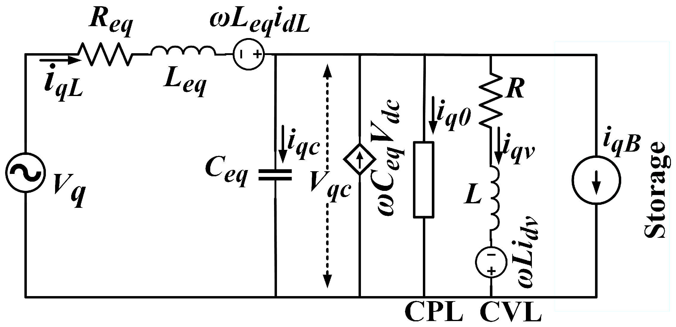
2. Modeling Microgrid with CPL

To mitigate purturbation caused by CPL loads, a compensation technique at the load side is the rational choice rather than compensating at the feeder side or using the intermediate circuitry approach. The load side compensation technique does required manipulation at the load side of the system to shield it from experiencing the effects caused by constant power loads. To elucidate this method, schematic models of storage-based real power compensation and reactive power compensation techniques (load side) are presented below in Figure 4 and Figure 5 [18].

From the dq-axis models demonstrated above, the combined state space equation of the espoused load side compensation technique is shown in Equation (1) [19].

$$\left[\begin{array}{c}\frac{d{i}_{dL}}{dt}\\ \frac{d{i}_{qL}}{dt}\\ \frac{d{V}_{dC}}{dt}\\ \frac{d{V}_{qC}}{dt}\\ \frac{d{i}_{dV}}{dt}\\ \frac{d{i}_{qV}}{dt}\end{array}\right]=\left[\begin{array}{c}\omega i_{qL}-\frac{R_1}{L_1}{i}_{dL}-\frac{V_{dc}}{L_1}+\frac{V_d}{L_1}\\ -\omega i_{dL}-\frac{R_1}{L_1}{i}_{qL}-\frac{V_{qc}}{L_1}+\frac{V_q}{L_1}\\ \omega V_{qC} + \frac{1}{C}{i}_{dL}- \frac{1}{C} \frac{P_O}{V_{dC}} - \frac{1}{C}{i}_{dV}-\frac{1}{C}{i}_{dB}\\ -\omega V_{dC} + \frac{1}{C}{i}_{qL}- \frac{1}{C} \frac{Q_O}{V_{qc}} - \frac{1}{C}{i}_{qV}-\frac{1}{C}{i}_{qB}\\ \omega i_{qV} + \frac{1}{L}{V}_{dC}- \frac{R}{L}{i}_{dV}\\ -\omega i_{dV} + \frac{1}{L}{V}_{qC}- \frac{R}{L}{i}_{qV}\end{array}\right],$$

(1)

3. Introduction to SMC and LRC

Sliding Mode Control (SMC) is a type of Variable Structure Control (VSC) in control theory. It gets switched from one continuous structure to a different one, based on the current state-space location. That makes SMC a variable structure control method. Its various control structures are configured to move the trajectories to a switching condition all the time, and therefore, the final trajectory will not be wholly within a single control structure. Instead of that, the final trajectory will slide along the control structure boundaries. The system’s motion while sliding along such boundaries is known as a Sliding Mode. The geometrical locus involving the boundaries is known as the sliding (hyper) surface. The sliding surface is defined by σ = 0, and after the limited time when the trajectories of the system have reached the surface, the sliding mode along the surface begins.

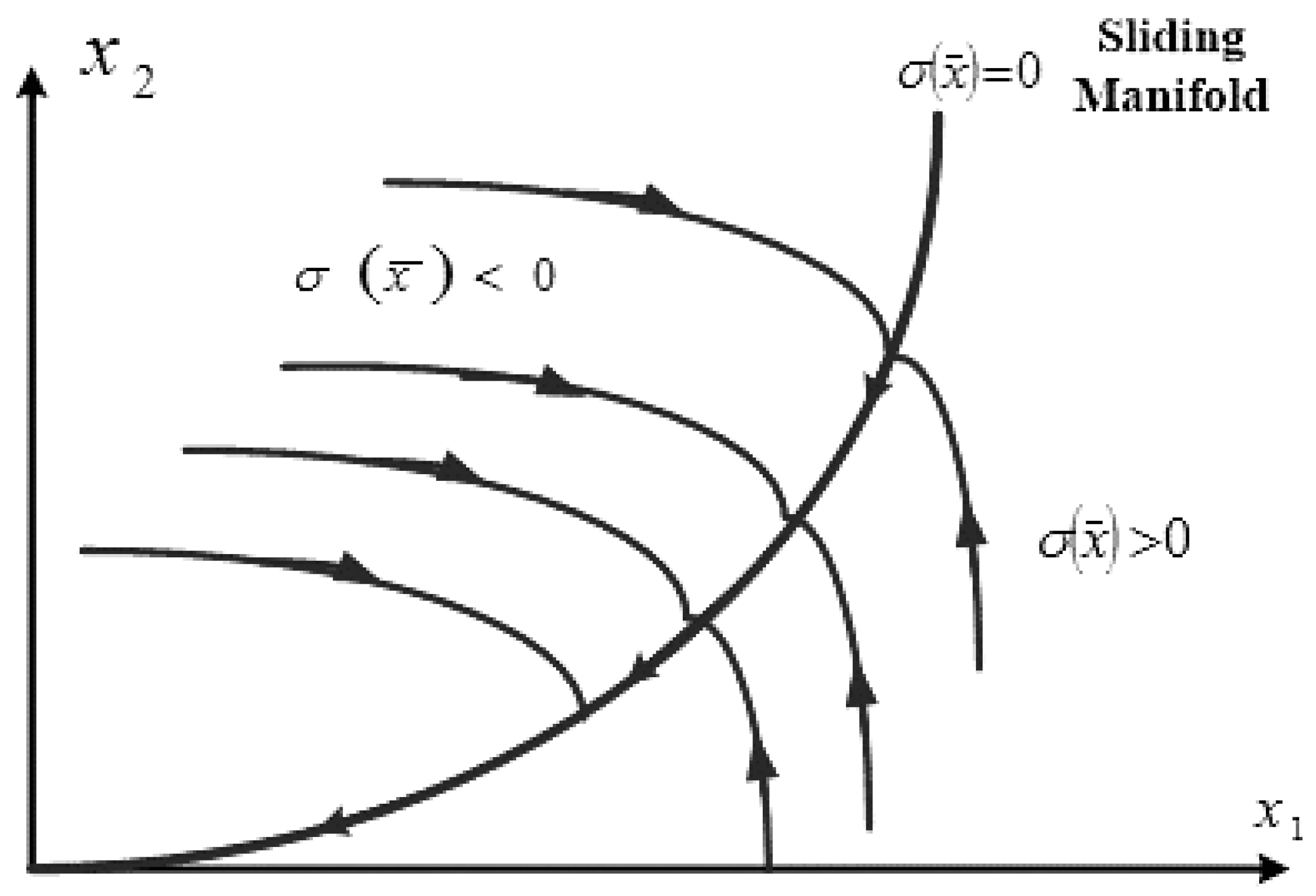
3.1. Sliding Mode Controller (SMC)

3.1.1. Control Statement of Sliding Mode

Considering a nonlinear dynamic system affine in control:

$$\dot{\overline{x}}\hspace{0.17em}(t)=f\hspace{0.17em}(\overline{x},t)+B\hspace{0.17em}(\overline{x})\hspace{0.17em}\overline{u}\hspace{0.17em}(t),$$

(2)

$$\overline{x}(t)\in {\Re }^n,\overline{u}(t)\in {\Re }^m,f(\overline{x},t)\in {\Re }^n,B(\overline{x})\in {\Re }^{nxm}$$

(3)

The components of the discontinuous feedback are given by:

$$u_i\hspace{0.17em}(t)=\{\begin{array}{l}{u}_i^{+}\hspace{0.17em}(\overline{x},t)\hspace{1em}if\hspace{0.17em}{\sigma }_i(x)>0\\ u_i^{-}\hspace{0.17em}(\overline{x},t)\hspace{1em}if\hspace{0.17em}{\sigma }_i(x)<0\end{array}\hspace{1em}i=1,2,\cdots ,m,$$

(4)

where σ_i(x) = 0 is the i-th component of the sliding surface, and $\sigma (x)={\left[{\sigma }_1(x),{\sigma }_2(x),\cdots ,{\sigma }_m(x)\right]}^T=0$ is the (n − m) dimensional sliding manifold. The sliding mode control structure includes selecting a manifold or a hypersurface (i.e., the sliding surface) so that the system trajectory demonstrates desired performance when restricted within this manifold, and finding discontinuous feedback gains to make the trajectory of the system intersect and stay on the manifold. Vicinity of the switching surface can be viewed from Figure 6.

A sliding mode exists, given that in the environs of the switching surface, σ(x) = 0, the state trajectory’s velocity vector, $\dot{\overline{x}}\hspace{0.17em}(t)$, is always directed toward the switching surface. The control laws of the sliding mode not being continuous, it is able of driving trajectories to the sliding mode in finite time (i.e., the sliding surface’s stability is superior to asymptotic). Nevertheless, the character of the sliding mode is taken on by the system (e.g., on this surface, the origin x = 0 can only possess asymptotic stability) once the trajectories reach the sliding surface.

3.1.2. Chattering

Due to the presence of external disturbance—noise and inertia of the sensors and actuators—the switching around the sliding surface occurs at a very high (but finite) frequency. The main consequence is that the sliding mode occurs in a small vicinity of the sliding manifold, which is called boundary layer, and which has a dimension that is inversely proportional to the control switching frequency. The effect of high frequency switching is known as chattering (shown in Figure 7).

The high-frequency switching propagate through the system exciting the fast dynamics and undesired oscillations that affect the system output. To prevent the chattering effect different techniques are used. One of the techniques is the use of continuous approximations of sign(.) using sat(.) or tanh(.) function in the implementation of the control law. A consequence of this method is that the invariance property is lost.

3.1.3. Chattering Reduction

Nowadays, typical approaches have been developed to reduce the amount of chattering. Slotine [43,44,45] based their original proposal on the generalized event of the nth-order single input variant of nonlinear system: $x^{(n)}=f\hspace{0.17em}(x,t)+B\hspace{0.17em}(x,t)\hspace{0.17em}u\hspace{0.17em}$; here x is the state variable; $x=[x,\dot{x},\stackrel{\dot{}\dot{}}{x},\dots ,x^{(n-1)}]$; x⁽ⁿ⁾ is the x’s nth-order derivative; B is the gain; f is a nonlinear function and u is the control input. Furthermore, a formula for the switching manifold of the above system and the distance between the state trajectory: s, is stated as: $s(t)={(\frac{d}{dt}+\lambda )}^{(n-1)}\tilde{x}$; while λ > 0 is a design constant, and $\tilde{x}$ is the tracking error defined as: $\tilde{x}=x-x_d$; whereas x_d is the state variable for the desired trajectory. Henceforth the corresponding switching manifold is: $s(t)=0$. Meanwhile, Slotine also proposed to smooth the previously mentioned discontinuity via a thin boundary layer closely surrounding the switching manifold. In such case continuous control within this boundary layer was attained by changing the switching term in the control law to a saturation function. Although the system would be driven to the boundary layer, yet the trajectory would not be staying on the switching manifold and thus the sliding mode would not exist [46]. Later Hung and Gao [47] offered the technique of reaching mode and reaching law, which was based upon nth-order m-input systems. To guarantee the state trajectory’s attraction towards the switching manifold within the reaching mode, their suggestion was to control the reaching speed by applying certain reaching law. They put forward three certain kinds of reaching laws besides the general form. Among these types they claimed that the power rate reaching law would eliminate chattering and provide fast reaching as well: ${\stackrel{•}{s}}_i=-k_i|s_i{|}^{\alpha }\mathit{sgn}(s_i)$. The reaching time T_i was deduced to: $T_i=\frac{|s_i(0){|}^{1-\alpha }}{(1-\alpha )k_i},i=1,2,\dots ,m$; where ${\stackrel{•}{s}}_i$ was the reaching speed; ${\stackrel{•}{s}}_i$ was defined as according to Equations (6) and (7); ${\stackrel{•}{s}}_i$ (0) was the initial value of ${\stackrel{•}{s}}_i$; k_i >0 was the switching gain (in the i-th dimension), and 0 < α < 1. Yet typically it has been found that chattering cannot be totally eliminated by such method. The above approaches are bounded by defects. Besides, Luo & Feng’s switching zone [48] appears mainly theoretical, whereas the Ground Validation System (GVS) of Hamerlan et al will have minimal effect on speed and position of the controlled subject [49].

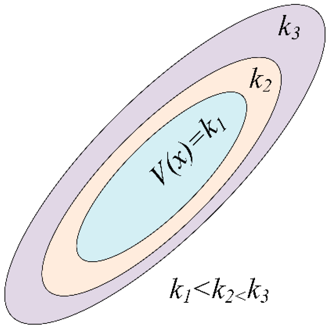
3.2. Lyapunov Redesign Controller (LRC)

Unlike sliding mode controller (SMC), Lyapunov redesign controller, or LRC, is based only on Lyapunov function [50,51]. Consider a nonlinear system that is described by:

$$\dot{x}=f(x)+G(x)u,$$

(5)

where $x\in {\Re }^n$ is the state and $u\in {\Re }^m$ is the controlled input. Assuming the matrix G(x) and the vector field ƒ(x) each has two components: an unknown part and a known nominal part. Therefore,

$$f(x)=f_0(x)+f^{*}(x),$$

(6)

$$G(x)=G_0(x)+G^{*}(x),$$

(7)

where ƒ₀ and G₀ represent the known nominal plant, and ƒ*, G* characterize the uncertainty. Later let us assume the unknown portion to conform to a certain bounding condition. Additionally, it is assumed that the uncertainty fulfills a so-called matching condition:

$$f^{*}(x)=G_0(x){\Delta }_{\dot{f}}(x),$$

(8)

$$G^{*}(x)=G_0(x){\Delta }_{\dot{G}}(x),$$

(9)

The matching condition suggests that terms of uncertainty are present in the same equations with the control inputs u, and consequently, it will be possible to control them by controller. By replacing (6)−(9) in (5) we obtain:

$$\dot{x}=f_0(x)+G_0(x)(u+\eta (x,u)),$$

(10)

which includes all of the uncertainty terms, and is defined by:

$$\eta (x,u)={\Delta }_{\stackrel{*}{f}}+{\Delta }_{\stackrel{*}{G}}u,$$

(11)

The Lyapunov redesign method works on the ensuing problem: supposing the equilibrium of the nominal model $\dot{x}=f(x)+G(x)u$ been made asymptotically stable uniformly by employing a feedback control law u = p₀(x), the goal is to devise a control function p*(x), which is corrective in nature, so that the enhanced control law u = p₀(x) + p*(x) can stabilize the system (defined by Equation (10)) faced by the uncertainty (x, u) getting constrained by a known function.

Then, let us think about the specifics of the Lyapunov redesign technique, that is comprehensively offered for a more common case. Let us assume a control law: u = p₀(x) to exist so that x = 0 becomes a stable equilibrium point which is uniformly asymptotically of the closed-loop nominal system $\dot{x}=f(x)+G_0(x)p_0(x)$. We also assume to know a Lyapunov function V₀(x) that fulfills:

$${\alpha }_1(||x||)\le V_0(x)\le {\alpha }_2(||x||),$$

(12)

$$\frac{\partial V_0}{\partial x}[f(x)+G_0(x)p_0(x)]\le -{\alpha }_3(\Vert x\Vert ),$$

(13)

where ${\alpha }_1,{\alpha }_2,{\alpha }_3:{\Re }^{+}\to {\Re }^1$ are stringently increasing functions that satisfy α_i(0) = 0 and α_i(r) → ∞ as r → ∞. These types of functions are sometimes called as class K_∞ functions. The term of uncertainty is presumed to satisfy the bound

$$||\eta (x,u)|{|}_{\infty }\le \stackrel{\_}{\eta }(t,x),$$

(14)

where the bounding function $\stackrel{\_}{\eta }$ is presumed to be known ‘a priori’, or accessible for measurement. At this point, let us proceed to designing the corrective “control component” p*(x) so that the system classes described by (10) and conforming to (14) are stabilized by u = p₀ + p*. An approach adhering to the nominal Lyapunov function V₀ is used as the base to design the corrective control term, thus the name ‘Lyapunov redesign method’ is justified. Considering the exact same Lyapunov function V₀ guaranteeing the nominal closed-loop system’s asymptotic stability, let us think about the time derivative of V₀ which is alongside the solutions of the full system (10). We have:

$$\begin{array}{l}\dot{V_0}=\frac{\partial V_0}{\partial x}[f_0(x)+G_0(x)(u+\eta (x,u))]\\ =\frac{\partial V_0}{\partial x}[f_0(x)+G_0(x)p_0(x)]+\frac{\partial V_0}{\partial x}{G}_0(x)p^{*}(x)+\eta (x,u))\le -{\alpha }_3(\Vert x\Vert )+\omega {(x)}^T{p}^{*}(x)+\omega {(x)}^T\eta (x,u)\end{array}$$

(15)

where,

$$\omega (x)={[\frac{\partial V_0}{\partial x}{G}_0(x)]}^T\in {\Re }^m,$$

(16)

which is a recognized function. We obtain by taking limits:

$$\begin{array}{l}{\dot{V}}_0\le -{\alpha }_3(\Vert x\Vert )+{\displaystyle \sum _{i=1}^m}{\omega }_i(x)p_i^{*}(x)+\Vert \omega (x)\Vert 1\dot{||}\eta (x,u)|{|}_{\infty }\\ =-{\alpha }_3(\Vert x\Vert )+{\displaystyle \sum _{i=1}^m}{\omega }_i(x)p_i^{*}(x)+\stackrel{\_}{\eta }(x,t)|{\omega }_i(x)|)\end{array}$$

(17)

The second term at the right-hand side of (17) can be made equal to zero if $p_i^{*}(x)$ is taken as:

$$p_i^{*}(x)=-\stackrel{\_}{\eta }(x,t)\mathrm{sgn}({\omega }_i(x)),$$

(18)

Every term of the corrective control vector p*(x) is chosen to be of the form p*(x) = $\pm \stackrel{\_}{\eta }(x,t)$, where the sign of p*(x) is contingent on the sign of _i(x) and changes as _i(x) changes its sign. Substituting Equation (18) in Equation (17), the desired "stability" property is obtained.

${\dot{V}}_0\le -{\alpha }_3(||x||)$; which infers that the closed-loop system is stable asymptotically. The augmented control law u = p₀(x) + p*(x) is discontinuous since each element $p_i^{*}(x)$ is discontinuous at _i(x) = 0. Moreover, the discontinuity jump $\stackrel{\_}{\eta }(x,t)\to -\stackrel{\_}{\eta }(x,t)$ can have great magnitude if the bound of uncertainty $\stackrel{\_}{\eta }$ is large. As demonstrated earlier, chattering can be caused by discontinuities in the control law; hence smoothing the discontinuity is desirable and is expected to retain some degree the nice stability properties at the same time from the original discontinuous control law. It is achievable by replacing Equation (18) with

$$p_i^{*}(x)=-\stackrel{\_}{\eta }(x,t)\tanh (\frac{{\omega }_i(x)}{\epsilon }),$$

(19)

where ε > 0 is a small design constant. It can be noted with ε approaching zero, the function $\tanh (\frac{{\omega }_i}{\epsilon })$ gets converged to the sgn(_i) function, which is discontinuous. By substituting Equation (19) in Equation (17) we obtain:

$${\dot{V}}_0\le -{\alpha }_3(||x||)+\stackrel{\_}{\eta }(x,t)\sum _{i=1}^m(|{\omega }_i(x)|-{\omega }_i(x)\tanh (\frac{{\omega }_i(x)}{\epsilon })),$$

(20)

Using Lemma:

$${\dot{V}}_0\le -{\alpha }_3(||x||)+\epsilon mk\stackrel{\_}{\eta }(x,t),$$

(21)

${\alpha }_3$ being a strictly increasing class $k_{\infty }$ function, for all r > 0 and any uniformly bounded function $\stackrel{\_}{\eta }$, there can exist a sufficiently small ε, so that ${\dot{V}}_0\le 0$ for x outside of a region $D_{\epsilon }=\left\{x V(x) \le r\right\}$. Consequently, the trajectory becomes convergent to the invariant set D_ε. A Lyapunov function’s level surfaces are shown in Figure 8. It demonstrates the Lyapunov surfaces for increasing values of k. The condition ${\dot{V}}_0\le 0$ suggests that the a trajectory moves within the set ${\Omega }_k=\{x\in {\Re }^n|V(x)\le k\}$ when it crosses the Lyapunov surface V(x) = k, and it cannot ever come out. The trajectory moves to an inner Lyapunov surface with smaller values of k when V < 0. The Lyapunov surface V(x) = k reduces back to the origin as k decreases, which shows that the approach of the trajectory to the origin with progressing time.

4. Implementation and Robustness Analysis of SMC and LRC

The intended outputs, or control objectives of the proposed controllers (each of SMC and LRC controller) is:

Y1 = V_dC ≈ V_d ≈ 480 Volt

Y2 = V_qC ≈ V_q ≈ (the lowest possible) Volt

Equation (22) gives the general system form affined within the control(s):

$$\dot{x}=f(x)+g(x)u,$$

(22)

4.1. Implementation and Robustness Analysis of Sliding Mode Controller against Parametric Uncertainties Including Uncertainties in Power of CPL

Sliding mode control, or SMC, is an advanced non-linear control technique featuring prominent characteristics of accuracy, robustness, and ease of tuning. By using the discontinuous control signal that forces the output of the system to ‘slide’ along with sliding surface or a distinct cross-section of the minimal behavior of the system, it can adjust the dynamics of the system in a way [47]. The state feedback control law is a discontinuous time function here, and can shift from one structure to the next depending on the prevailing location in space in a continuous manner. Hence, sliding mode control can be described as a control technique with variable structures. As the system’s certain operation mode slides along the predetermined control structure boundaries, it is called the sliding mode. The geometrical locus, which consists of the boundaries, is called the system’s sliding surface. To implement the sliding mode controller, the state space model equation below can be rewritten as Equation (23). In this section, the robustness will be enhanced by considering the uncertainties in active power of CPL $(P_0)$ and reactive power of CPL $(Q_0)$. When $P_0$ is unknown in case of designing $u_1$, we will also consider $x_3$ as unknown to avoid any complexity. Similarly, in case of $u_2$, we will also consider $x_4$ as unknown.

$$\left[\begin{array}{c}\dot{x_1}\\ \dot{x_2}\\ \dot{x_3}\\ \dot{x_4}\\ \dot{x_5}\\ \dot{x_6}\end{array}\right]=\left[\begin{array}{c}\omega x_2-\frac{R_1}{L_1}{x}_1-\frac{x_3}{L_1}\\ -\omega x_1-\frac{R_1}{L_1}{x}_2-\frac{x_4}{L_1}\\ \omega x_4 + \frac{1}{C}{x}_1- \frac{1}{C}\frac{P_0}{x_3} - \frac{1}{C}{x}_5\\ -\omega x_3 + \frac{1}{C}{x}_2- \frac{1}{C}\frac{Q_0}{x_4} - \frac{1}{C}{x}_6\\ \omega x_6 + \frac{1}{L}{x}_3- \frac{R}{L}{x}_5\\ -\omega x_5 + \frac{1}{L}{x}_4- \frac{R}{L}{x}_6\end{array}\right]+\left[\begin{array}{c}0\\ 0\\ -\frac{1}{C}{u}_1\\ -\frac{1}{C}{u}_2\\ 0\\ 0\end{array}\right]+\left[\begin{array}{c}\frac{r_1}{L_1}\\ \frac{r_2}{L_1}\\ 0\\ 0\\ 0\\ 0\end{array}\right],$$

(23)

Although $P_0$ and $Q_0$ are unknown, they satisfy $P_0\le {\delta }_P$ and $Q_0\le {\delta }_Q$ for some known bounds ${\delta }_P$ and ${\delta }_Q$. The variation on CPL power can be summarized as:

$$d_P={\Delta }_P/ \Delta x_3,$$

(24)

$$d_Q={\Delta }_Q/ \Delta x_4,$$

(25)

where $d_P$ represents the uncertainties of $P_0$, $d_Q$ represents the uncertainties of $Q_0$, $\Delta x_3$ is the uncertainties in $x_3$, and $\Delta x_4$ is the uncertainties in $x_4$. As $x_3$ and $x_4$ are in the denominator, we need lower bounds of these parameters. Power uncertainty is expressed in term of current. We know that $x_3$ is the voltage of “d-axis” and it satisfies $\Delta x_3\le {\delta }_{x3}$ for some known, stringently positive bound ${\delta }_{x3}$. Similarly, $x_4$ is the “q-axis” voltage. It satisfies $\Delta x_4\le {\delta }_{x4}$ for some known, stringently positive bound ${\delta }_{x4}$. Overall, there are six unknowns with known bounds. The Sliding Mode Control input, $u_1$ will be designed first, with the similar method adopted to design $u_2$, the other control input. Using the similar method as discussed in the previous section, let

$$e_1={\displaystyle \int }(x_3-x_{3d})dt,$$

(26)

$$e_2={\dot{e}}_1=x_3-x_{3d},$$

(27)

$${\dot{e}}_2={\dot{x}}_3-{\dot{x}}_{3d} =f_3(x)+g_3(x)u_1-{\dot{x}}_{3d},$$

(28)

Expanding $f_3(x)$ and $g_3(x)$

$${\dot{e}}_2=\omega x_4+\frac{1}{c}{x}_1-\frac{1}{c}\frac{P_0}{x_3}-\frac{1}{c}{x}_5-\frac{1}{c}{u}_1-{\dot{x}}_{3d},$$

(29)

Let, the sliding surface be

$$s=e_1+e_2,$$

(30)

After differentiating and considering the uncertainties:

$$\dot{s}={\dot{e}}_1+{\dot{e}}_2,$$

(31)

$$\dot{s}=e_2+(\omega ({\widehat{x}}_4+\Delta x_4)+\frac{1}{c}({\widehat{x}}_1+\Delta x_1)-\frac{1}{c}(\frac{P_0}{x_3}+d_P)-\frac{1}{c}{x}_5-\frac{1}{c}{u}_1-{\dot{x}}_{3d}),$$

(32)

where $x_{4 }={\widehat{x}}_4+\Delta x_4$. Then the total parametric uncertainty including uncertainty of CPL power can be represented as:

$$d=\frac{1}{c}\Delta x_1+\omega \Delta x_4-\frac{1}{c}{d}_P; \Vert d\Vert \le dmax,$$

(33)

here $dmax$ is the limit of the total disturbance d.

$$dmax= \frac{1}{c}{\delta }_{x1}+\omega {\delta }_{x4}- \frac{1}{c}{\delta }_P/ {\delta }_{x3},$$

(34)

Then,

$$\dot{s}=e_2-\frac{1}{c}{x}_5-{\dot{x}}_{3d}+\omega {\widehat{x}}_4+\frac{1}{c}{\widehat{x}}_1-\frac{1}{c}\frac{P_0}{x_3}-\frac{1}{c}{u}_1+d,$$

(35)

Let it be considered as the Lyapunov candidate function.

$$V=\frac{1}{2}{s}^2,$$

(36)

$$\dot{V}=s\dot{s}=s(e_2-\frac{1}{c}{x}_5-{\dot{x}}_{3d}+\omega {\widehat{x}}_4+\frac{1}{c}{\widehat{x}}_1-\frac{1}{c}\frac{P_0}{x_3}-\frac{1}{c}{u}_1+d),$$

(37)

We use $u_1$.

$$u_1=-c\left[-e_2+\frac{1}{c}{x}_5+{\dot{x}}_{3d}-\omega {\widehat{x}}_4-\frac{1}{c}{\widehat{x}}_1+\frac{1}{c}\frac{P_0}{x_3}+v\right],$$

(38)

Now, we can obtain:

$$\dot{V}=s(d+v),$$

(39)

$\Vert d\Vert \le dmax,$ put into consideration, $\dot{V}$ will be made negative by the subsequent discontinuous control, $v$. Consequently, it will guarantee stability.

$$v=-dmax\ast sat\left(\frac{s}{\epsilon }\right); \epsilon >0,$$

(40)

In total, the control input is:

$$u_1=-c\left[-e_2+\frac{1}{c}{x}_5+{\dot{x}}_{3d}+\frac{1}{c}\frac{P_0}{x_3}-\omega {\widehat{x}}_4-\frac{1}{c}{\widehat{x}}_1-dmax*sat\left(\frac{s}{\epsilon }\right) \right],$$

(41)

Such an analysis is also presented here for $u_2$, let,

$$e_3={\displaystyle \int }(x_4-x_{4d})dt,$$

(42)

$$e_4={\dot{e}}_3=x_4-x_{4d},$$

(43)

$${\dot{e}}_4={\dot{x}}_4-{\dot{x}}_{4d}=f_4(x)+g_4(x)u_2-{\dot{x}}_{4d},$$

(44)

Taking the sliding surface as:

$$s=e_3+e_4,$$

(45)

After differentiation and considering the uncertainties:

$$\dot{s}=e_4+\left(-\omega ({\widehat{x}}_3+\Delta x_3)+\frac{1}{c}({\widehat{x}}_2+\Delta x_2)-\frac{1}{c}(\frac{Q_0}{x_4}+d_Q)-\frac{1}{c}{x}_6-\frac{1}{c}{u}_2-{\dot{x}}_{4d}\right),$$

(46)

where $x_{3 }={\widehat{x}}_3+\Delta x_3$. Then the total parametric uncertainty including uncertainty of CPL power can be represented as:

$$d=\frac{1}{c}\Delta x_2-\omega \Delta x_3-\frac{1}{c}{d}_Q; \Vert d\Vert \le dmax,$$

(47)

where $dmax$ is the limit for d, the total disturbance.

$$dmax= \frac{1}{c}{\delta }_{x2}-\omega {\delta }_{x3}- {\delta }_Q/{\delta }_{x4},$$

(48)

Then,

$$\dot{s}=e_3-\frac{1}{c}{x}_6-{\dot{x}}_{4d}+\omega {\widehat{x}}_3+\frac{1}{c}{\widehat{x}}_2-\frac{1}{c}\frac{Q_0}{x_4}-\frac{1}{c}{u}_2+d,$$

(49)

Considering this as the Lyapunov candidate function:

$$V=\frac{1}{2}{s}^2,$$

(50)

$$\dot{V}=s\dot{s}=s(e_3-\frac{1}{c}{x}_6-{\dot{x}}_{4d}+\omega {\widehat{x}}_3+\frac{1}{c}{\widehat{x}}_2-\frac{1}{c}\frac{Q_0}{x_4}-\frac{1}{c}{u}_2+d),$$

(51)

We then use $u_2$.

$$u_2=-c\left[-e_3+\frac{1}{c}{x}_6+{\dot{x}}_{4d}-\omega {\widehat{x}}_3-\frac{1}{c}{\widehat{x}}_2+\frac{1}{c}\frac{Q_0}{x_4}+v\right],$$

(52)

Then, we can obtain:

$$\dot{V}=s(d+v),$$

(53)

Considering $\Vert d\Vert \le dmax,$ $\dot{V}$ will be made negative by the subsequent discontinuous control, $v$. Consequently, it will guarantee stability.

$$v=-dmax\ast sat\left(\frac{s}{\epsilon }\right); \epsilon >0,$$

(54)

In total, the control input is:

$$u_2=-c\left[-e_3+\frac{1}{c}{x}_6+{\dot{x}}_{4d}-\omega {\widehat{x}}_3-\frac{1}{c}{\widehat{x}}_2+\frac{1}{c}\frac{Q_0}{x_4}-dmax\ast sat\left(\frac{s}{\epsilon }\right)\right],$$

(55)

4.2. Implementation and Robustness Analysis of Lyapunov Redesign Controller against Parametric Uncertainties Including Uncertainties in Power of CPL

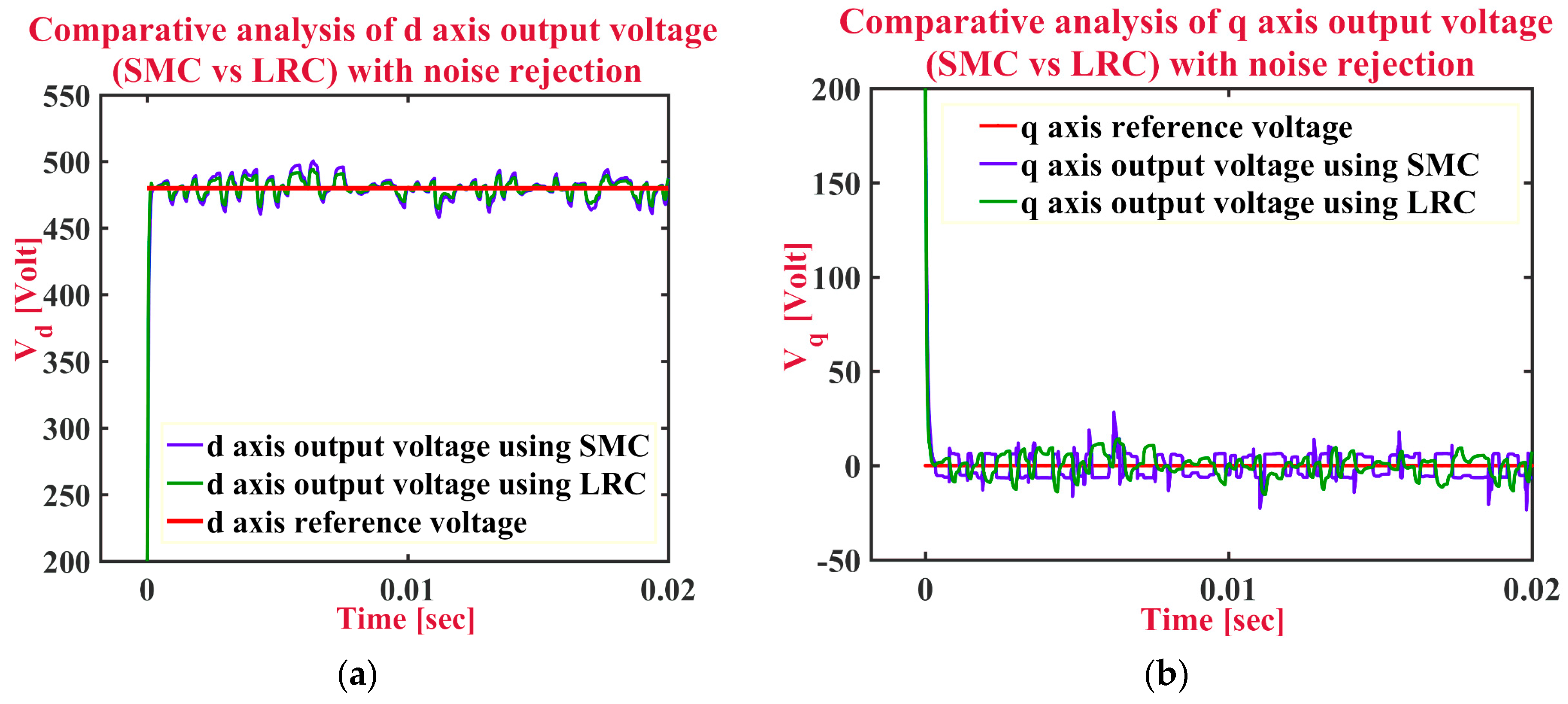
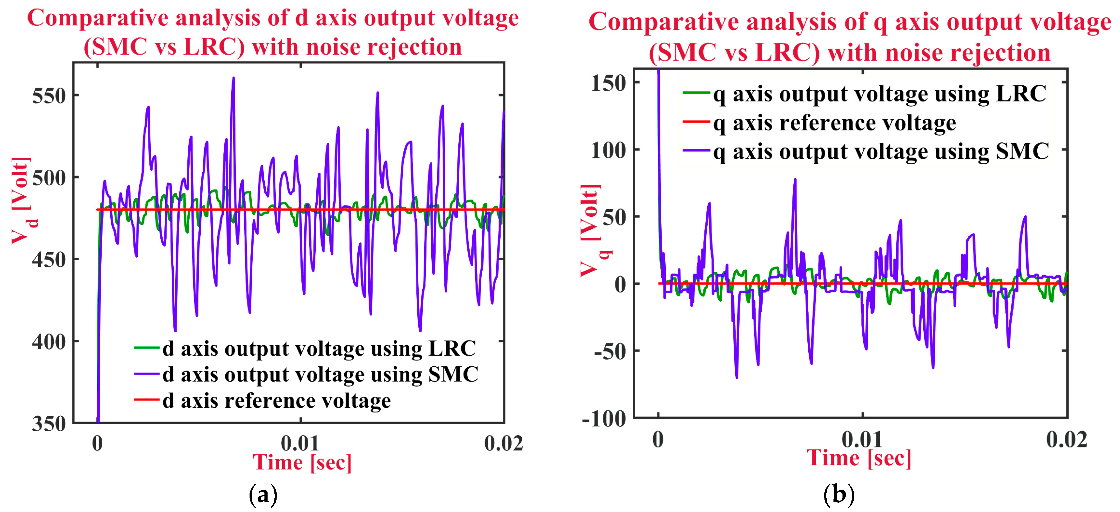
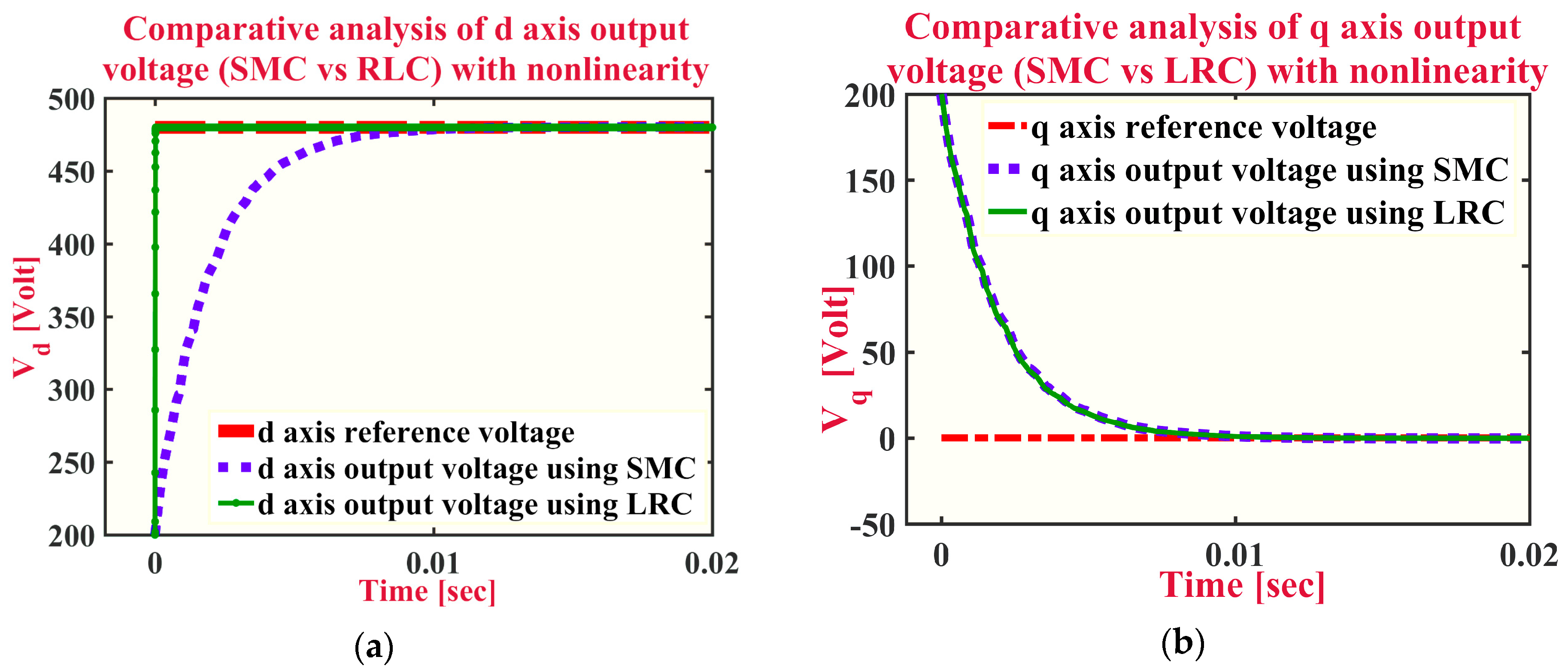
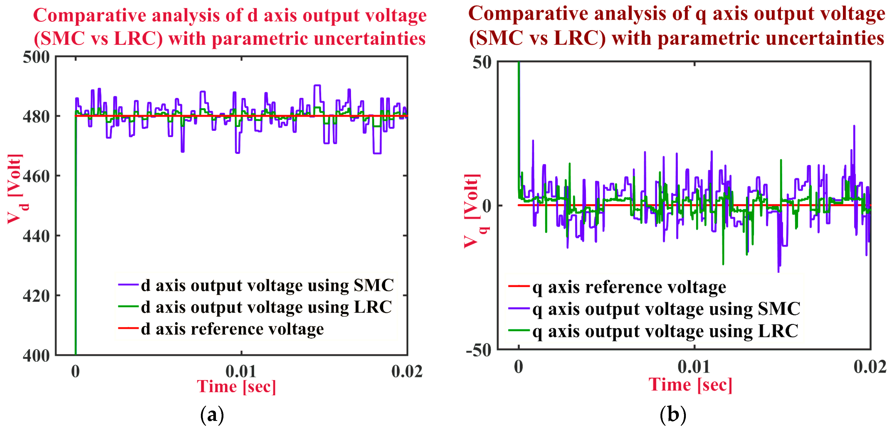
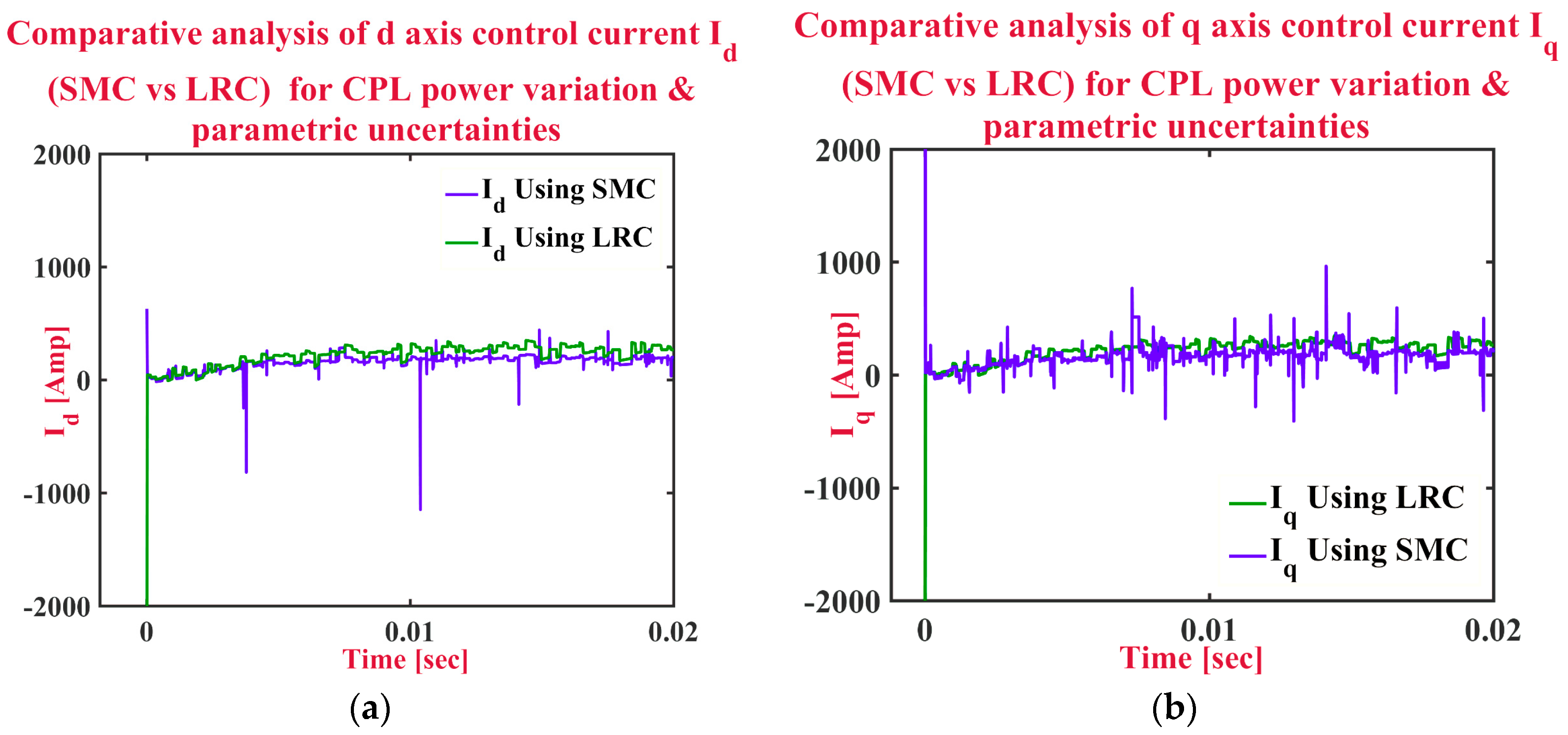
The LRC is based only on Lyapunov function. Its nominal controller is designed to ensure the nominal system or disturbance-free system to be stable by forcing the Lyapunov function derivative of the nominal system to be negative. If there is disturbance in the system, the discontinuous control is used alone to handle the disturbance. The discontinuous controller is formulated by redesigning the Lyapunov function of the nominal system. In the redesigning process, the disturbance is introduced to the Lyapunov function of the nominal system and then solved for the discontinuous control to overcome that disturbance and force the new derivative Lyapunov function or be negative and consequently, the system to be globally stable. It has some chattering issues because of the discontinuous controller. The chattering magnitude is dependent on the magnitude of dmax. Having large dmax makes the system stable against large disturbance but it can cause larger chattering if it is set as a very large value. If the disturbance happens to be greater than the set dmax, the system can become unstable. But, the LRC has greater margin for stability because its nominal system is also ensured to be stable, thus provides better performance for large disturbance.

First of all, the Lyapunov Redesign Control input, $u_1$ will be designed, with the same approach followed next to design the other control input, $u_2$. Using the similar method as discussed in last section, we introduce new state variables:

$$e_1={\displaystyle \int }(x_3-x_{3d})dt,$$

(56)

$$e_2={\dot{e}}_1=x_3-x_{3d},$$

(57)

$${\dot{e}}_2={\dot{x}}_3-{\dot{x}}_{3d} =f_3(x)+g_3(x)u_1-{\dot{x}}_{3d},$$

(58)

Expanding $f_3(x)$ and $g_3(x)$:

$${\dot{e}}_2=\omega x_4+\frac{1}{c}{x}_1-\frac{1}{c}\frac{P_0}{x_3}-\frac{1}{c}{x}_5-\frac{1}{c}{u}_1-{\dot{x}}_{3d},$$

(59)

Considering the uncertainties:

$${\dot{e}}_2=\omega ({\widehat{x}}_4+\Delta x_4)+\frac{1}{c}({\widehat{x}}_1+\Delta x_1)-\frac{1}{c}\left(\frac{P_0}{x_3}+d_P\right)-\frac{1}{c}{x}_5-\frac{1}{c}{u}_1-{\dot{x}}_{3d},$$

(60)

Then the total parametric uncertainty including uncertainty of CPL power can be represented as:

$$d=\frac{1}{c}\Delta x_1+\omega \Delta x_4-\frac{1}{c}{d}_P; \Vert d\Vert \le dmax,$$

(61)

here $dmax$ is the limit of d, the total disturbance.

$$dmax= \frac{1}{c}{\delta }_{x1}+\omega {\delta }_{x4}- \frac{1}{c}{\delta }_P/ {\delta }_{x3},$$

(62)

Following the methodology of Lyapunov redesign, the over-all input is $u_1=u_0+v$; where $u_0$ is the nominal stabilizing controller and $v$ is to handle the disturbances. We get the linear state space of error as in Equation (63):

$$\dot{e}=\left[\begin{array}{cc}0& 1\\ -k_1& -k_2\end{array}\right]e,$$

(63)

Now, we define the desired Eigen values for the linearized system. Desired Eigen values would be −10.

Let, Equation (63) be written as $\dot{e}=Ae$ and $A=\left[\begin{array}{cc}0& 1\\ -k_1& -k_2\end{array}\right]$

Generalized Eigen values of matrix “A”:

$$sI-A=\left[\begin{array}{cc}s& -1\\ k_1& s+k_2\end{array}\right],$$

(64)

$$|sI-A|=s^2+k_{2}s+k_1,$$

(65)

Characteristic polynomial (desired):

$$(s+10)(s+10)=s^2+20s+100,$$

(66)

Comparing Equations (65) and (66):

$$k_2=20, k_1=100$$

So, the values of $k_1$ and $k_2$ will become +100 and +20 respectively.

$$\dot{e}=\left[\begin{array}{cc}0& 1\\ -100& -20\end{array}\right]e,$$

(67)

$$A=\left[\begin{array}{cc}0& 1\\ -100& -20\end{array}\right],$$

(68)

$$PA+A^{T}P=-I,$$

(69)

$$P=\left[\begin{array}{cc}\frac{21}{8}& \frac{1}{200}\\ \frac{1}{200}& \frac{101}{4000}\end{array}\right],$$

(70)

$$V(e)=e^{T}Pe,$$

(71)

$$w=2e^{T}PG=2\left[\begin{array}{cc}{e}_1& e_2\end{array}\right]\left[\begin{array}{cc}\frac{21}{8}& \frac{1}{200}\\ \frac{1}{200}& \frac{101}{4000}\end{array}\right]\left[\begin{array}{c}0\\ 1\end{array}\right],$$

(72)

$$w=\frac{1}{100}{e}_1+\frac{101}{2000}{e}_2,$$

(73)

Then, we can choose the Lyapunov function for the nominal system or disturbance-free system to be:

$$V=\frac{1}{2}{e}_2^2,$$

(74)

$$\dot{V}=e_2{\dot{e}}_2=e_2\left(\omega {\widehat{x}}_4+\frac{1}{c}{x}_1-\frac{1}{c}\frac{P_0}{x_3}-\frac{1}{c}{x}_5-\frac{1}{c}{u}_0-{\dot{x}}_{3d}\right),$$

(75)

If we choose,

$$u_0=-c\left[\frac{1}{c}\frac{P_0}{x_3}-\omega {\widehat{x}}_4+\frac{1}{c}{x}_5+{\dot{x}}_{3d}-k_1{e}_1-k_2{e}_2\right],$$

(76)

then, $\dot{V}<0$. The terms $\left[-k_1{e}_1-k_2{e}_2\right]$ guarantee the global stability of the nominal system which is absent in SMC method. The overall system is stabilized using the discontinuous control in the presence of disturbances. Redesigning the Lyapunov function considering disturbances,

$$V=\frac{1}{2}{e}_2^2,$$

(77)

$$\dot{V}=e_2{\dot{e}}_2=e_2(\left(\omega {\widehat{x}}_4+\frac{1}{c}{x}_1-\frac{1}{c}\frac{P_0}{x_3}-\frac{1}{c}{x}_5-\frac{1}{c}{u}_0-{\dot{x}}_{3d}\right)+\left(\frac{1}{c}v+d\right)),$$

(78)

$\left[\omega {\widehat{x}}_4+\frac{1}{c}{x}_1-\frac{1}{c}\frac{P_0}{x_3}-\frac{1}{c}{x}_5-\frac{1}{c}{u}_0-{\dot{x}}_{3d} \right]$ is assured to be negative, then the discontinuous control can be designed as:

$$v=-c\ast dmax\ast sat(\frac{dmax\ast \omega }{\mu }),$$

(79)

Then, the overall input is:

$$u_1=-c\left[\frac{1}{C}\frac{P_0}{x_3}-\omega {\widehat{x}}_4+\frac{1}{C}{x}_5+{\dot{x}}_{3d}-100e_1-20e_2-dmax\ast sat\left(\frac{dmax\left(\frac{1}{100}{e}_1+\frac{101}{2000}{e}_2\right)}{\mu }\right)\right],$$

(80)

Therefore, there is $\mu >0$ so that for $\mu <{\mu }^{\ast }$, the closed-loop system’s origin is asymptotically stable globally according to absolute stability theorem. Similarly, we have Equation (81), when we design a controller for u₂ with same desired points.

$$u_2=-c\left[\frac{1}{C}\frac{Q_0}{x_4}+\omega {\widehat{x}}_3+\frac{1}{C}{x}_6+{\dot{x}}_{4d}-100e_3-20e_4-dmax\ast sat\left(\frac{dmax\left(\frac{1}{100}{e}_3+\frac{101}{2000}{e}_4\right)}{\mu }\right)\right],$$

(81)

where,

$$e_3={\displaystyle \int }(x_4-x_{4d})dt,$$

(82)

$$e_4={\dot{e}}_3=x_4-x_{4d},$$

(83)

$$d=\frac{1}{c}\Delta x_2-\omega \Delta x_3-\frac{1}{c}{d}_Q; \Vert d\Vert \le dmax= \frac{1}{c}{\delta }_{x2}-\omega {\delta }_{x3}-{\delta }_Q/ {\delta }_{x4},$$

(84)

5. Results

Here, the parameters and the parametric values regarding the simulation done for comparative analysis by varying the CPL power have been shown in

Table 1. Table of Parameters.

Parameter	Value	Parameter	Value
$\Omega$	$60 \mathrm{Hz}$	${\delta }_{x4}$	$100 \mathrm{V}$
X3	$600 \mathrm{V}$	${\delta }_P$	$30 \mathrm{kW}$
X4	50 V	${\delta }_Q$	$2 \mathrm{kVar}$
$d_P$	50 A	${\rho }_{x3}$	$200 \mathrm{V}$
$d_Q$	20 A	$\epsilon$	$100$
${\delta }_{x3}$	$1000 \mathrm{A}$	$Req$	$0.25 \mathrm{Ohm}$
$Leq$	0.5 × 10−3 H	$Ceq$	10 × 10−6 F
RCVL	15 Ohm	LCVL	5 × 10−3 H
RB	10 Ohm	CB	1 × 10−6 F
LB	1 × 10−3 H

.

In Figure 9a,b, performance comparisons have been illustrated between SMC (colored in blue) and LRC (colored in green) for d-axis output voltage and q-axis output voltage respectively. The control objective for d-axis output voltage has been considered as 480 Volt, for normal conditions—where the variance value has been set as 10% to simulate noise. From Figure 9a, it is evident that the LRC controller shows considerably superior performance than that of the SMC controller, as its output stayed closer to the control objective. For q-axis output voltage, the control objective has been considered as low as possible and negligible in practice. In Figure 9b, the q-axis output voltage fluctuates more in the case of the SMC controller than that of the LRC controller. To determine the controller behaviors in a very noisy environment, more noise is added by setting the variance value as 100%, and noise rejection capabilities of SMC and LRC are tested. The results are shown in Figure 10a,b, which demonstrate LRC’s superior capability to stick to the reference value with close proximity, whereas SMC has fluctuations of great magnitudes. For nonlinearity, LRC is capable of attaining the reference d-axis value with negligible time-delay, but SMC needs some time to reach that (Figure 11a). However, for q-axis, both controllers exhibit a similar performance (Figure 11b). In case of parametric uncertainties, LRC again proves to be the better suited one, displaying less fluctuations than SMC to maintain the control objective (Figure 12a,b). Hence, LRC offers appreciable stability considering CPL power variation and parametric uncertainties. In Figure 13a,b, performance comparisons have been presented between SMC (blue colored) and LRC (green colored) in the case of d-axis control input current, I_d (u₁) and q-axis control input current, I_q (u₂) respectably considering CPL power variation and parametric uncertainties. Here, the more the fluctuation in control input current, the more the stress will be imposed on the storage system to compensate, consequently degrading the storage performance and overall life time. This situation, in practice, makes it harder to retain microgrid stability. The mean squared errors (MSE) obtained from these analyses for both SMC and LRC controllers are presented in

Table 2. Mean squared error (MSE) values of SMC and LRC controllers for the different conditions.

Conditions	Parameter	Mean Squared Error		Relative Error (SMC-LRC)
		SMC	LRC
Noise Rejection (normal condition)	X3, d-axis voltage	0.00270320	0.00139074	1.31246 × 10−3
	X4, q-axis voltage	0.00138790	0.00113038	2.5752 × 10−4
Noise Rejection (very noisy condition)	X3, d-axis voltage	0.03661991	0.00139411	3.52258 × 10−2
	X4, q-axis voltage	0.00818637	0.00112001	7.06636 × 10−3
Nonlinearity	X3, d-axis voltage	0.00321589	0.00002730	3.18859 × 10−3
	X4, q-axis voltage	0.00942499	0.00924679	1.782 × 10−4
Parameter Uncertainty	X3, d-axis voltage	0.00116666	0.00011259	1.04076 × 10−3
	X4, q-axis voltage	0.00126333	0.00017554	1.08779 × 10−3

. It is obvious from the presented values that LRC is the better controller, and in a noisy environment, SMC is no match for LRC, as the former displays error significantly greater than LRC. This observation also leads to believe that, for practical applications, LRC can provide better performance than LRC. Therefore, from the comparative analysis presented here, the Lyapunov Redesign Controller shows better performance to retain system stability in face of CPL power variation. Hence, the LRC controller is preferred to be adopted for storage-based load side compensation technique for microgrid stability improvement with dense CPL loads present.

6. Reason behind Inferior SMC Performance and Solutions

Sliding Mode Control presents many fascinating challenges to the mathematicians. It is also extensively used in engineering applications because of the comparatively easy implementation which does not require a deep understanding of the complex mathematical background. These two reasons put it in a unique position among control theories. There are three main stages of designing a Sliding Mode Controller: designing the sliding surface, selecting the control law that will hold the system trajectory on the sliding surface, and implementing in a chatter-free setup—which is the most important one of these three. Although in theory, Sliding Mode Control is a robust one, experiments show otherwise—SMC has some serious shortcomings. The most prominent one of them is chattering—the high frequency oscillation around the sliding surface. It reduces the control performance significantly. As an example, the following second-order system can be considered:

$${\dot{x}}_1=x_2,$$

(85)

$${\dot{x}}_2=a{x}_1+b{x}_2+csin{x}_1+du,$$

(86)

a and b are negative constant values here whereas c and d are positive constants. For c > |a|, the system is known to be unstable. For the actuator, existence of fast dynamics is posited, and it is stable. These are not considered in the ideal model. The equations governing them are:

$$w_1=w,$$

(87)

$${\dot{w}}_1=w_2,$$

(88)

$${\dot{w}}_2=-\frac{1}{{\mu }^2}{w}_1-\frac{2}{\mu }{w}_2+\frac{1}{{\mu }^2}u,$$

(89)

μ is a constant, considered to have a positive, sufficiently small value. As demonstrated in Figure 14, with actuator unmodeled dynamics present, $w(t)$ is the actual input of the system, not u(t) directly from the sliding mode controller. The sliding mode surface and the control input is chosen as:

$$u=-Msign(\sigma ),$$

(90)

$$\sigma =\lambda x_1+x_2,$$

(91)

where λ and M are positive constants, with M is required to be large enough to enforce sliding mode into the ideal model $(\dot{\sigma }\sigma >0)$. $\dot{x}$ becomes a continuous time function in real system, thus making the expectation of sliding mode to occur invalid; and causes chatter.

According to theory, the unmodeled dynamics present in the system causes the chattering effect. A sliding mode control, which is “chattering free”, is not attainable as the model used in designing the controller can never capture all the system dynamics. But, the chattering can be curtailed. The sliding mode is normally implemented with a relay—which represents the sign function. It creates a common problem with relative degree equal to one. An alternative to this approach is using approximations of the sign function, which is widely used. Sigmoids, saturation, and hysteresis functions are used often too, providing a continuous or smooth control signal, but also losing the invariance property of the sliding mode control along the way.

Table 3. Methods to improve SMC technique.

Technique Name	Base of the Technique	Working Principle	Effectiveness
ISMC	Has a equal dimension to the state space	Control signal composed by a linear term with a continuous low excitation of the unmodeled dynamics	**
HOSM	High-gain control with saturations used for overcoming the effect of chattering by approximation of the sign function within a boundary layer around the switching manifold	The order of the mode is determined by the smoothness of tangency of the sliding manifold	**
T2FNNAS	Type-2 Fuzzy Neural Network	Based on the synthesis method Lyapunov, the adaptive FNN’s free parameters are tuned on-line	***
SMESO	Extended state observer with active disturbance rejection control	Dramatically reduced chattering phenomenon on the control input channel with respect to Linear Extended State Observer	**
FSMC	Low pass filter	Estimation of the sliding variable via a disturbance estimator	*

*** = Excellent, ** = Satisfactory, * = Acceptable.

shows some methods to improve the effectiveness of SMC. Fuzzy Sliding Mode Control (FSMC)—which uses a low pass filter, and estimates the sliding variable through a disturbance estimator—is the one with the least effectiveness. Integral Sliding Mode Control (ISMC), High Order Sliding Mode (HOSM), and Sliding Mode Extended State Observer (SMESO) offers better effectiveness. However, Type-2 Fuzzy-Neural Network Indirect Adaptive Sliding Mode Control (T2FNNAS) is the way to achieve the best performance, which is based on the synthesis approach of Lyapunov [52,53].

7. Numerical Verification of Results for Microgrid Application

The results obtained so far demonstrate the capabilities of both SMC and LRC to maintain microgrid stability. To ascertain the effectiveness of these methods in real-life conditions, both of them are simulated numerically with data obtained from physical microgrids. These simulations confirm the efficacy of these control systems to sustain stability in real microgrids.

7.1. SMC Technique

To verify the global stability, we have to calculate the equation below:

$$\dot{V}=s(d+v),$$

(92)

where,

$$d=\frac{1}{c}\Delta x_1+\omega \Delta x_4-\frac{1}{c}{d}_P,$$

(93)

$$v=-dmax\ast sat\left(\frac{s}{\epsilon }\right); \epsilon >0,$$

(94)

So,

$$\dot{V}= s\left(\frac{1}{c}\Delta x_1+\omega \Delta x_4-\frac{1}{c}{d}_P-dmax\ast sat\left(\frac{s}{\epsilon }\right)\right),$$

(95)

where,

$$dmax= \frac{1}{c}{\delta }_{x1}+\omega {\delta }_{x4}- \frac{1}{c}{\delta }_P/ {\delta }_{x3},$$

(96)

Putting these all together,

$$\dot{V}= s\left(\frac{1}{c}\Delta x_1+\omega \Delta x_4-\frac{1}{c}{d}_p-\left(\frac{1}{c}{\delta }_{x1}+\omega {\delta }_{x4}- \frac{1}{c}{\delta }_P/ {\delta }_{x3}\right)\ast sat\left(\frac{s}{\epsilon }\right)\right),$$

(97)

Now let,

$$\omega = 60 \mathrm{Hz}, \Delta x_1 = 200 \mathrm{A}, \Delta x_4 = 50 \mathrm{V}, d_P = 50 \mathrm{A}, {\delta }_{x1} = 4000 \mathrm{A}, {\delta }_{x3} = 100 \mathrm{A}, {\delta }_{x4} = 100 \mathrm{V},$$

$${\delta }_P = 30 \mathrm{kW}, \epsilon = 100, c= 10 \mathsf{\mu }\mathrm{F}$$

Putting these values, we get:

$$\dot{V}= s\left(\frac{1}{10\mu }(200)+(60)(50)-\frac{1}{10\mu }(50)-\left(\frac{1}{10\mu }(4000)+(60)(100)- \frac{1}{10\mu }\left(\frac{30k}{100}\right)\right)\ast sat\left(\frac{\mathrm{s}}{100}\right)\right),$$

(98)

$$\dot{V} = s\left[15.003 \times {10}^6 - [370.006 \times {10}^6]sat\left(\frac{s}{100}\right)\right],$$

(99)

Now, if s is either positive or negative, we will obtain $\dot{V} \le 0$, which guarantees global stability.

7.2. LRC Technique

We have,

$$\dot{V}=e_2{\dot{e}}_2,$$

(100)

where,

$${\dot{e}}_2=\left(\omega x_4+\frac{1}{c}{x}_1-\frac{1}{c}\frac{P_0}{x_3}-\frac{1}{c}{x}_5-\frac{1}{c}{u}_0-{\dot{x}}_{3d}\right)+\left(\frac{1}{c}v+d\right),$$

(101)

And here,

$$v=-c\ast dmax\ast sat(\frac{dmax\ast w}{\mu }),$$

(102)

$$d=\Delta \omega n_4+\Delta \omega x_4+\omega n_4+\frac{1}{c}\Delta x_1-\frac{1}{c}(n_5+\Delta x_5)-\frac{1}{c}{d}_P ,$$

(103)

And,

$$dmax=\frac{1}{c}{\delta }_{x1}+ {\delta }_{\omega }{\delta }_{n4}+{\delta }_{\omega }{\delta }_{x4}+\omega {\delta }_{n4} -\frac{1}{c}{\delta }_5- \frac{1}{c}{\delta }_P/ {\delta }_{x3},$$

(104)

If we choose

$$u_0=-c\left[\frac{1}{c}\frac{P_0}{x_3}-\omega {\widehat{x}}_4+\frac{1}{c}{x}_5+{\dot{x}}_{3d}-k_1{e}_1-k_2{e}_2\right],$$

(105)

Putting it all together,

$$\dot{V}=e_2\left(\left(\omega x_4+\frac{1}{c}{x}_1-\frac{1}{c}\frac{P_0}{x_3}-\frac{1}{c}{x}_5-\frac{1}{c}{u}_0-{\dot{x}}_{3d}\right)+\left(\frac{1}{c}\left(-c\ast dmax\ast sat(\frac{dmax\ast w}{\mu })\right)+(\Delta \omega n_4+\Delta \omega x_4+\omega n_4+\frac{1}{c}\Delta x_1-\frac{1}{c}(n_5+\Delta x_5)-\frac{1}{c}{d}_P)\right)\right),$$

(106)

$$\dot{V}=e_2\left(\right(\omega x_4+\frac{1}{c}{x}_1-\frac{1}{c}\frac{P_0}{x_3}-\frac{1}{c}{x}_5-\frac{1}{c}(-c\left[\frac{1}{c}\frac{P_0}{x_3}-\omega {\widehat{x}}_4+\frac{1}{c}{x}_5+{\dot{x}}_{3d}-k_1{e}_1-k_2{e}_2\right])-{\dot{x}}_{3d})+(\frac{1}{c}(-c\ast \left(\frac{1}{c}{\delta }_{x1}+{\delta }_{\omega }{\delta }_{n4}+{\delta }_{\omega }{\delta }_{x4}+\omega {\delta }_{n4}-\frac{1}{c}{\delta }_5-\frac{1}{c}{\delta }_P/ {\delta }_{x3}\right)\ast sat\left(\frac{\left(\frac{1}{c}{\delta }_{x1}+ {\delta }_{\omega }{\delta }_{n4}+{\delta }_{\omega }{\delta }_{x4}+\omega {\delta }_{n4} -\frac{1}{c}{\delta }_5- \frac{1}{c}{\delta }_P/ {\delta }_{x3}\right)\ast w}{\mu }\right))+(\Delta \omega n_4+\Delta \omega x_4+\omega n_4+\frac{1}{c}\Delta x_1-\frac{1}{c}(n_5+\Delta x_5)-\frac{1}{c}{d}_P)))$$

(107)

Now let,

$\omega =60 \mathrm{Hz}, x_3=600 \mathrm{V}, x_4=10 \mathrm{V},\Delta x_1=200 \mathrm{A}$, $\Delta x_2=200 \mathrm{A}$, $\Delta x_5=10 \mathrm{A},$ $n_3=50 \mathrm{V},$ $n_4=50 \mathrm{V},$ $n_5=30 \mathrm{A}, n_6=30 \mathrm{A}, \Delta \omega =10 \mathrm{Hz}, d_P=50 \mathrm{A}, d_Q=20 \mathrm{A}$, ${\delta }_{x1}=4000 \mathrm{A}$, ${\delta }_{x3}=200 \mathrm{A}$, ${\delta }_{x4}=100 \mathrm{V}$, ${\delta }_{\omega }=70 \mathrm{Hz}$, ${\delta }_P=30 \mathrm{kW}$, ${\delta }_Q=20 \mathrm{Var}, {\delta }_{n3}= {\delta }_{n4}={\delta }_{n5}={\delta }_{n6}=100 \mathrm{A},$ ${\rho }_{x3}=200 \mathrm{V},$ and $\mu =100$, ${\delta }_{x5}=50 \mathrm{A}, {\delta }_{x6}=3 \mathrm{A}$, ${\delta }_5=150 \mathrm{A}$ and ${\delta }_6=13 \mathrm{A}$, $c=10 \mathsf{\mu }\mathrm{F}$.

Putting the values, we get:

$$\dot{V}=e_2((-(100)(600-480)-(20)(0))+(\frac{1}{10\mu }(-10\mu \ast \left(\frac{1}{10\mu }(4000)+(70)(100)+(70)(100)+(60)(100) -\frac{1}{10\mu }(150)- \frac{1}{10\mu }\left(\frac{30k}{200}\right)\right)\ast sat\left(\frac{\left(\frac{1}{10\mu }(4000)+(70)(100)+(70)(100)+(60)(100) -\frac{1}{10\mu }(150)- \frac{1}{10\mu }\left(\frac{30k}{200}\right)\right)\ast (60)}{100}\right))+((10)(50)+(10)(10)+(60)(50)+\frac{1}{10\mu }(100)-\frac{1}{10\mu }(30+10)-\frac{1}{10\mu }(50))\left)\right),$$

(108)

$$\dot{V}=e_2[988900-[370.02\times {10}^6]\ast sat(222.012\times {10}^6)]$$

(109)

As we are getting $\dot{V} \le 0$ from this equation, the system is globally stable.

8. Conclusions

A microgrid system has several advantages over the conventional utility grid system, such as unlimited renewable fuel resources, environment-friendly power generation, easy implementation, cost effectiveness, and so on. However, the maintenance of the microgrid electrification has been confronted by the challenge of continually increasing instability issues due to the growth of modern electronic devices. For improving the stability scenario of the microgrid system despite the presence of dense CPL loads, a storage-based load side compensation technique has been adopted in this paper. Besides that, Sliding Mode Controller (SMC) and Lyapunov Redesign Controller (LRC), two of the most prominent nonlinear control techniques, have been implemented individually to retain microgrid system stability. After that, SMC and LRC controller robustness analysis have been presented with the variation of CPL power. Next, the comparative analysis between the SMC controller and the LRC controller robustness has been illustrated which ascertains that Lyapunov Redesign Controller has a superior performance than the former one to retain microgrid stability in dense CPL-loaded conditions. Reasons for inferior SMC performance and ways to overcome them have been discussed afterwards, followed by numerical analysis of both of the control techniques to verify their performance in real microgrids. All the necessary results have been simulated in Matlab/Simulink platform with appreciable aftermath.

References

1. Bayindir, R.; Hossain, E.; Kabalci, E.; Perez, R. A comprehensive study on microgrid technology. Int. J. Renew. Energy Res. 2014, 4, 1094–1107. [Google Scholar]
2. Hossain, E.; Kabalci, E.; Bayindir, R.; Perez, R. Microgrid testbeds around the world: State of art. Energy Convers. Manag. 2014, 86, 132–153. [Google Scholar] [CrossRef]
3. Reddy, K.R.; Babu, N.R.; Sanjeevikumar, P. A review on grid codes and reactive power management in power grids with wecs. In Advances in Smart Grid and Renewable Energy; Springer: Berlin, Germany, 2018; pp. 525–539. [Google Scholar]
4. Un-Noor, F.; Padmanaban, S.; Mihet-Popa, L.; Mollah, M.N.; Hossain, E. A comprehensive study of key electric vehicle (ev) components, technologies, challenges, impacts, and future direction of development. Energies 2017, 10, 1217. [Google Scholar] [CrossRef]
5. Ganesan, S.; Padmanaban, S.; Varadarajan, R.; Subramaniam, U.; Mihet-Popa, L. Study and analysis of an intelligent microgrid energy management solution with distributed energy sources. Energies 2017, 10, 1419. [Google Scholar] [CrossRef]
6. AL-Nussairi, M.K.; Bayindir, R.; Padmanaban, S.; Mihet-Popa, L.; Siano, P. Constant power loads (cpl) with microgrids: Problem definition, stability analysis and compensation techniques. Energies 2017, 10, 1656. [Google Scholar] [CrossRef]
7. Mihet-Popa, L.; Isleifsson, F.; Groza, V. Experimental Testing for Stability Analysis of Distributed Energy Resorces Components with Storage Devices and Loads. In Proceedings of the 2012 IEEE International Instrumentation and Measurement Technology Conference, Graz, Austria, 13–16 May 2012; pp. 588–593. [Google Scholar]
8. Mihet-Popa, L.; Han, X.; Bindner, H.; Pihl-Andersen, J.; Mehmedalic, J. Development and Modeling of different scenarios for a Smart Distribution Grid. In Proceedings of the 2013 IEEE 8th International Symposium on Applied Computational Intelligence and Informatics, Timisoara, Romania, 23–25 May 2013; pp. 257–261. [Google Scholar]
9. Mihet-Popa, L.; Zong, Y.; You, S.; Groza, V. Simulation Platform Developed to Study and Identify Critical Cases in a Future Smart Grid. In Proceedings of the 2016 IEEE Electrical Power and Energy Conference (EPEC), Ottawa, ON, Canada, 12–14 October 2016. [Google Scholar]
10. Camacho, O.M.F.; Nørgård, P.B.; Rao, N.; Mihet-Popa, L. Electrical Vehicle Batteries Testing in a Distribution Network using Sustainable Energy. IEEE Trans. Smart Grid 2014, 5, 1033–1042. [Google Scholar] [CrossRef]
11. Emadi, A.; Khaligh, A.; Rivetta, C.H.; Williamson, G.A. Constant power loads and negative impedance instability in automotive systems: Definition, modeling, stability, and control of power electronic converters and motor drives. IEEE Trans. Veh. Technol. 2006, 55, 1112–1125. [Google Scholar] [CrossRef]
12. Jelani, N.; Molinas, M.; Bolognani, S. Reactive power ancillary service by constant power loads in distributed ac systems. IEEE Trans. Power Deliv. 2013, 28, 920–927. [Google Scholar] [CrossRef]
13. Rahimi, A.M.; Williamson, G.A.; Emadi, A. Loop-cancellation technique: A novel nonlinear feedback to overcome the destabilizing effect of constant-power loads. IEEE Trans. Veh. Technol. 2010, 59, 650–661. [Google Scholar] [CrossRef]
14. Huddy, S.R.; Skufca, J.D. Amplitude death solutions for stabilization of dc microgrids with instantaneous constant-power loads. IEEE Trans. Power Electron. 2013, 28, 247–253. [Google Scholar] [CrossRef]
15. Kwasinski, A.; Onwuchekwa, C.N. Dynamic behavior and stabilization of dc microgrids with instantaneous constant-power loads. IEEE Trans. Power Electron. 2011, 26, 822–834. [Google Scholar] [CrossRef]
16. Sanchez, S.; Molinas, M. Large signal stability analysis at the common coupling point of a dc microgrid: A grid impedance estimation approach based on a recursive method. IEEE Trans. Energy Convers. 2015, 30, 122–131. [Google Scholar] [CrossRef]
17. Wu, M.; Lu, D.D.-C. A novel stabilization method of lc input filter with constant power loads without load performance compromise in dc microgrids. IEEE Trans. Ind. Electron. 2015, 62, 4552–4562. [Google Scholar] [CrossRef]
18. Hossain, E.; Perez, R.; Nasiri, A.; Bayindir, R. Development of lyapunov redesign controller for microgrids with constant power loads. Renew. Energy Focus 2017, 19, 49–62. [Google Scholar] [CrossRef]
19. Hossain, E.; Perez, R.; Padmanaban, S.; Siano, P. Investigation on the development of a sliding mode controller for constant power loads in microgrids. Energies 2017, 10, 1086. [Google Scholar] [CrossRef]
20. Singh, S.; Fulwani, D.; Kumar, V. Robust sliding-mode control of dc/dc boost converter feeding a constant power load. IET Power Electron. 2015, 8, 1230–1237. [Google Scholar] [CrossRef]
21. Padmanaban, S.; Ozsoy, E.; Fedák, V.; Blaabjerg, F. Development of sliding mode controller for a modified boost ćuk converter configuration. Energies 2017, 10, 1513. [Google Scholar] [CrossRef]
22. Stramosk, V.; Pagano, D.J. Nonlinear control of a bidirectional dc-dc converter operating with boost-type constant-power loads. In Proceedings of the 2013 Brazilian Power Electronics Conference (COBEP), Gramado, Brazil, 27–31 October 2013; IEEE: Piscataway, NJ, USA, 2013; pp. 305–310. [Google Scholar]
23. Gautam, A.R.; Singh, S.; Fulwani, D. DC bus voltage regulation in the presence of constant power load using sliding mode controlled DC-DC bi-directional converter interfaced storage unit. In Proceedings of the 2015 IEEE First International Conference on DC Microgrids (ICDCM), Atlanta, GA, USA, 7–10 June 2015; IEEE: Piscataway, NJ, USA, 2015; pp. 257–262. [Google Scholar]
24. Singh, S.; Fulwani, D. On design of a robust controller to mitigate CPL effect—A DC micro-grid application. In Proceedings of the 2014 IEEE International Conference on Industrial Technology (ICIT), Busan, Korea, 26 February–1 March 2014; IEEE: Piscataway, NJ, USA, 2014; pp. 448–454. [Google Scholar]
25. Padmanaban, S.; Blaabjerg, F.; Wheeler, P.; Ojo, J.O.; Ertas, A.H. High-voltage dc-dc converter topology for pv energy utilization—Investigation and implementation. Electr. Power Compon. Syst. 2017, 45, 221–232. [Google Scholar] [CrossRef]
26. Liu, Z.; Liu, J.; Bao, W.; Zhao, Y. Infinity-norm of impedance-based stability criterion for three-phase ac distributed power systems with constant power loads. IEEE Trans. Power Electron. 2015, 30, 3030–3043. [Google Scholar] [CrossRef]
27. Emadi, A. Modeling of power electronic loads in ac distribution systems using the generalized state-space averaging method. IEEE Trans. Ind. Electron. 2004, 51, 992–1000. [Google Scholar] [CrossRef]
28. Sun, J. Small-signal methods for ac distributed power systems—A review. IEEE Trans. Power Electron. 2009, 24, 2545–2554. [Google Scholar]
29. Karimipour, D.; Salmasi, F.R. Stability analysis of ac microgrids with constant power loads based on popov’s absolute stability criterion. IEEE Trans. Circuits Syst. II Express Briefs 2015, 62, 696–700. [Google Scholar] [CrossRef]
30. Vavilapalli, S.; Padmanaban, S.; Subramaniam, U.; Mihet-Popa, L. Power balancing control for grid energy storage system in photovoltaic applications—Real time digital simulation implementation. Energies 2017, 10, 928. [Google Scholar] [CrossRef]
31. Swaminathan, G.; Ramesh, V.; Umashankar, S.; Sanjeevikumar, P. Investigations of microgrid stability and optimum power sharing using robust control of grid tie pv inverter. In Advances in Smart Grid and Renewable Energy; Springer: Singapore, 2018; pp. 379–387. [Google Scholar]
32. Zheng, Q.; Wu, F. Lyapunov redesign of adaptive controllers for polynomial nonlinear systems. In Proceedings of the American Control Conference (ACC ’09), St. Louis, MO, USA, 10–12 June 2009; IEEE: Piscataway, NJ, USA, 2009; pp. 5144–5149. [Google Scholar]
33. Chung, W.-C.; Liaw, D.-C.; Chang, S.-T. The steering control of vehicle dynamics via a lyapunov redesign approach. In Proceedings of the 48th IEEE Conference on Decision and Control, 2009 Held Jointly with the 2009 28th Chinese Control Conference (CDC/CCC 2009), Shanghai, China, 15–18 December 2009; IEEE: Piscataway, NJ, USA, 2009; pp. 6321–6326. [Google Scholar]
34. Memon, A.Y.; Khalil, H.K. Lyapunov redesign approach to output regulation of nonlinear systems using conditional servocompensators. In Proceedings of the American Control Conference, Seattle, WA, USA, 11–13 June 2008; IEEE: Piscataway, NJ, USA, 2008; pp. 395–400. [Google Scholar]
35. Farrell, J.A.; Polycarpou, M.M. Adaptive Approximation Based Control: Unifying Neural, Fuzzy and Traditional Adaptive Approximation Approaches; John Wiley & Sons: Chichester, UK, 2006; Volume 48. [Google Scholar]
36. Khalil, H.K. Noninear Systems; Prentice-Hall: Upper Saddle River, NJ, USA, 1996; Volume 2. [Google Scholar]
37. Vilathgamuwa, D.; Zhang, X.; Jayasinghe, S.; Bhangu, B.; Gajanayake, C.; Tseng, K.J. Virtual resistance based active damping solution for constant power instability in ac microgrids. In Proceedings of the IECON 2011—37th Annual Conference on IEEE Industrial Electronics Society, Melbourne, Australia, 7–10 November 2011; IEEE: Piscataway, NJ, USA, 2011; pp. 3646–3651. [Google Scholar]
38. Tiwari, R.; Babu, N.R.; Arunkrishna, R.; Sanjeevikumar, P. Comparison between pi controller and fuzzy logic-based control strategies for harmonic reduction in grid-integrated wind energy conversion system. In Advances in Smart Grid and Renewable Energy; Springer: Berlin, Germany, 2018; pp. 297–306. [Google Scholar]
39. Padmanaban, S.; Grandi, G.; Blaabjerg, F.; Wheeler, P.W.; Siano, P.; Hammami, M. A comprehensive analysis and hardware implementation of control strategies for high output voltage dc-dc boost power converter. Int. J. Comput. Int. Syst. 2017, 10, 140–152. [Google Scholar] [CrossRef]
40. Padmanaban, S.; Daya, F.J.; Blaabjerg, F.; Wheeler, P.W.; Szcześniak, P.; Oleschuk, V.; Ertas, A.H. Wavelet-fuzzy speed indirect field oriented controller for three-phase ac motor drive–investigation and implementation. Eng. Sci. Technol. Int. J. 2016, 19, 1099–1107. [Google Scholar] [CrossRef]
41. Febin Daya, J.L.; Subbiah, V.; Iqbal, A.; Padmanaban, S. Novel wavelet-fuzzy based indirect field oriented control of induction motor drives. J. Power Electron. 2013, 13, 656–668. [Google Scholar] [CrossRef]
42. Febin Daya, J.; Subbiah, V.; Sanjeevikumar, P. Robust speed control of an induction motor drive using wavelet-fuzzy based self-tuning multiresolution controller. Int. J. Comput. Int. Syst. 2013, 6, 724–738. [Google Scholar] [CrossRef]
43. Slotine, J.-J.E.; Li, W. Applied Nonlinear Control; Prentice Hall: Englewood Cliffs, NJ, USA, 1991; Volume 199. [Google Scholar]
44. Slotine, J.-J.E. Sliding controller design for non-linear systems. Int. J. Control 1984, 40, 421–434. [Google Scholar] [CrossRef]
45. Utkin, V.I. Sliding Modes in Control and Optimization; Springer Science & Business Media: Berlin/Heidelberg, Germany, 2013. [Google Scholar]
46. Sastry, S.S. Nonlinear Systems: Analysis, Stability, and Control; Springer Science & Business Media: New York, NY, USA, 2013; Volume 10. [Google Scholar]
47. Hung, J.Y.; Gao, W.; Hung, J.C. Variable structure control: A survey. IEEE Trans. Ind. Electron. 1993, 40, 2–22. [Google Scholar] [CrossRef]
48. Ning-Su, L.; Chun-Bo, F. A new method for suppressing chattering in variable structure feedback control systems. IFAC Proc. Vol. 1989, 22, 279–284. [Google Scholar] [CrossRef]
49. Loh, A.M.; Yeung, L. Chattering reduction in sliding mode control: An improvement for nonlinear systems. WSEAS Trans. Circuits Syst. 2004, 3, 2090–2097. [Google Scholar]
50. Freeman, R.; Kokotovic, P.V. Robust Nonlinear Control Design: State-Space and Lyapunov Techniques; Springer Science & Business Media: Boston, MA, USA, 2008. [Google Scholar]
51. Krishna S, M.; Daya JL, F.; Padmanaban, S.; Mihet-Popa, L. Real-time analysis of a modified state observer for sensorless induction motor drive used in electric vehicle applications. Energies 2017, 10, 1077. [Google Scholar] [CrossRef]
52. Sanjeevikumar, P.; Febin Daya, J.L.; Wheeler, P.; Blaabjerg, F.; Fedák, V.; Ojo, J.O. Wavelet Transform with Fuzzy Tuning Based Indirect Field Oriented Speed Control of Three-Phase Induction Motor Drive. In Proceedings of the 2015 International Conference on Electrical Drives and Power Electronics (EDPE), Tatranska Lomnica, Slovakia, 21–23 September 2015; pp. 111–116. [Google Scholar]
53. Hosseyni, A.; Trabelsi, R.; Iqbal, A.; Sanjeevikumar, P.; Mimouni, M.F. An Improved Sensorless Sliding Mode Control/Adaptive Observer of a Five-Phase Permanent Magnet Synchronous Motor Drive. Int. J. Adv. Manuf. Technol. 2017, 93, 1–11. [Google Scholar] [CrossRef]
Figure 1. Negative impedance characteristic of constant power load.
Energies 10 01959 g001
Figure 2. Research timeline on Constant Power Load Compensation Techniques, considering the published research works.
Energies 10 01959 g002
Figure 3. Contributions of different countries on Constant Power Load Instability Compensation research.
Energies 10 01959 g003
Figure 4. Real power compensation method at the load side, modeled for d-axis.
Energies 10 01959 g004
Figure 5. Reactive power compensation method at the load side, modeled for q-axis.
Energies 10 01959 g005
Figure 6. Vicinity of the switching surface.
Energies 10 01959 g006
Figure 7. The chattering effect of Sliding Mode Controller (SMC).
Energies 10 01959 g007
Figure 8. A Lyapunov function’s level surfaces.
Energies 10 01959 g008
Figure 9. Comparison of performance between SMC (blue colored) and LRC (green colored) for normal condition in case of (a) d-axis output voltage; (b) q-axis output voltage considering CPL power variation and parametric uncertainties. LRC controller shows considerably better performance than SMC by staying closer to the reference voltage.
Energies 10 01959 g009
Figure 10. Comparison of performance between SMC (blue colored) and LRC (green colored) for very noisy environment in case of (a) d-axis output voltage; (b) q-axis output voltage considering CPL power variation and parametric uncertainties. LRC controller shows far better performance than SMC, as the latter shows high fluctuations from the reference voltage, while LRC stays close to it.
Energies 10 01959 g010
Figure 11. Comparison of performance between SMC (colored in blue) and LRC (colored in green) for nonlinearity in case of (a) d-axis output voltage, (b) q-axis output voltage. Unlike SMC, LRC is capable of attaining the reference d-axis value with negligible time-delay.
Energies 10 01959 g011
Figure 12. Comparison of performance between SMC (colored in blue) and LRC (colored in green) in case of (a) d-axis output voltage, (b) q-axis output voltage considering parametric uncertainties. LRC controller shows considerably better performance than SMC by staying closer to the reference voltage.
Energies 10 01959 g012
Figure 13. Comparison of performance among SMC (colored in blue) and LRC (colored in green) in case of (a) d-axis control input current, Id (u1); (b) q-axis control input current, Iq (u2) considering CPL power variation and parametric uncertainties. LRC fluctuated less than SMC, causing less stress on the system and thus providing a longer lifetime.
Energies 10 01959 g013
Figure 14. An example system demonstrating sliding mode control for systems as described in Equations (85) and (86). There are actuator dynamics that are not included in the ideal system. Chattering is caused from the excitation of these unmodeled dynamics by the high frequency switching action.
Energies 10 01959 g014