Identification of Power Transformer Winding Mechanical Fault Types Based on Online IFRA by Support Vector Machine


1
College of Engineering and Technology, Southwest University, Chongqing 400715, China
2
State Key Laboratory of Power Transmission Equipment & System Security and New Technology, School of Electrical Engineering, Chongqing University, Chongqing 400044, China
*
Author to whom correspondence should be addressed.
Energies 2017, 10(12), 2022; https://doi.org/10.3390/en10122022
Submission received: 13 November 2017
/
Revised: 28 November 2017
/
Accepted: 29 November 2017
/
Published: 1 December 2017
Abstract
:A transformer is the most valuable and expensive property for power utility, thus ensuring its reliable operation is a major task for both operators and researchers. Online impulse frequency response analysis has proven to be a promising technique for detecting transformer internal winding mechanical deformation faults when a power transformer is in service. However, as so far, there is still no reliable standard code for frequency response signature interpretation and quantification. This paper tries to utilize a machine learning method, namely the support vector machine, to identify and classify the winding mechanical fault types, based on online impulse frequency response analysis. Actual transformer fault data from a specially manufactured model transformer are collected and analyzed. Two feature vectors are proposed and the diagnostic results are predicted. The diagnostic results indicate the satisfied classifying accuracy by the proposed method.
1. Introduction
The power transformer is regarded as one of the most valuable facilities in power substations; it is significant to ensure its stable, reliable and safe operation [1]. However, the installation time of most power transformers worldwide dates back to the 1980s and they are reaching their deadline of designed life cycle [2,3]. It is also reported in many studies that the failure rate of power transformers has recently increased globally. Normally, transformer internal faults including the electrical insulation faults and the winding mechanical faults are key internal factors to induce the transformer failure. Winding mechanical faults, namely winding deformation (such as tilting, forced bulking, free buckling, hoop tension, telescoping, etc.), are difficult to detect at an early stage because they have limited impact on the normal operation of power transformers [4]. However, as the transformer continues to operate and suffers the external short circuit current, the minor winding mechanical fault would eventually develop catastrophic failure if no steps are taken. The condition monitoring technique makes it possible to detect the winding incipient mechanical faults when the transformer is in service [5,6]. Thus, it is tremendously necessary to timely detect and diagnose the winding mechanical deformation faults, especially with the online technique.
Frequency response analysis (FRA), firstly introduced by Dick and Erven [7], has been developed as a widely accepted tool for the last decades, due to its reliable, fast, economic, and non-destructive features [8]. The transformer winding is proven to be equivalent of an electrical network consisting of resistance, capacitance and inductance in high frequency range, and its frequency response signature can represent the status of the winding [9]. The first version of FRA, known as sweep frequency response analysis (SFRA), has adopted sweep frequency sinuous signal to excite transformer windings and measure the response signal in the frequency domain to construct a frequency response signature [10]. Afterwards, the other version of FRA, known as impulse frequency response analysis (IFRA), has emerged [11]. An impulse signal with wideband frequency spectrum has been used to excite the transformer windings and the response signal is measured in time domain, both signals are converted to frequency domain to construct a frequency response signature [12].
Recently, online SFRA and online IFRA have been burgeoned. Behjat realized the experimental application of online SFRA by a homemade noninvasive capacitor sensor (NICS), in combination with a network analyzer [13,14]. Bagheri studied the effect of the bushing tap capacitance on the online SFRA signature by connecting variable capacitive bushings to the tested windings [15]. For the online IFRA, Leibfried used the transient signal, which was caused by the switching operation, to excite transformer windings [16]; while Wang introduced the lightning over-voltage being the excitation signal of the online IFRA [17]. These two types of transient signals belong to the uncontrollable signal. Furthermore, by using controllable signals, Rybel proposed a method to online monitor the transformer by injecting the high frequency signal to the winding terminal through the bushing tap [18]. Then, Yao established a capacitive coupling sensor (CCS) and an other apparatus for injecting the nanosecond pulse to the transformer windings [19]. Besides, Zhao analyzed the impact of the capacitive coupling circuit on the online IFRA signature by theoretical analysis and experimental validation [20]. Compared with current SFRA, IFRA has the advantage of a high signal to noise ratio and smaller energy injection, which reaches the potential for online application.
Although there are extensive publications characterizing the online FRA, most of them focus on the implementation of the method itself. As so far, there is still no reliable standard code for both SFRA and IFRA signature identification and quantification [21,22]. FRA is a graphical analysis method; skilled personnel is required for the interpretation of FRA signatures. Moreover, there is little literature regarding the identification of winding faults in online IFRA. Rahimpour has divided the comparison algorithms of FRA signatures into four major categories: Algorithms based on exact calculations, algorithms based on estimation methods, algorithms based on electric circuit models and algorithms based on artificial methods [23]. Among these algorithms, artificial methods, such as genetic algorithm (GA), neural network (NN), support vector machine (SVM), are intelligent machine learning algorithms with high accuracy. Particularly, SVM has advantages of solving the classification problem of small-scale samples, non-linearity, and high-dimension. For the problem of classifying transformer winding mechanical deformation, it is not easy to collect actual FRA data for different winding deformation types, extent and location, especially for large power transformers, which makes SVM developing a suitable tool for solving this problem. Bigdeli proposed SVM to identify transformer winding faults based on the transfer function, and the verification process reveals the proposed method has a high accuracy [24]. However, this work involves offline FRA. With a view to the current status of online IFRA identification, this paper proposes the SVM algorithm to classify the transformer winding mechanical fault types, for the purpose of achieving the actual application of the online IFRA method.
2. Brief Introduction of Online Impulse Frequency Response Analysis
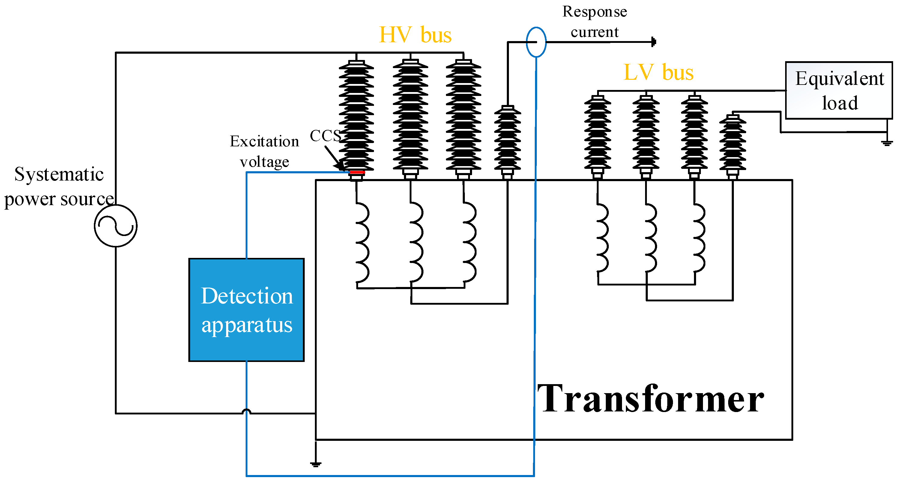
A simple diagram of the online IFRA method is depicted in Figure 1. The transformer is in service, with the systematic power source energized in the HV side and the load in the LV side. The controllable high voltage nanosecond pulses are injected into the terminal of the transformer winding by using a CCS, which is a metal strip that is wrapped around the bushing external insulation layer. Particularly, CCS functions as a medium to couple the nanosecond pulse voltage into the winding terminal. The usage of CCS has erased the low frequency data of online IFRA signature, and this effect can be found in [20,25]. The impact of CCS on bushing external insulation can be discovered in [26]. More detailed information about the diagnostic system and the practical application can be found in [19,27].
In the online IFRA test, both the excitation nanosecond pulse signals and the response pulse signals of windings are simultaneously recorded to construct the IFRA signature of a transformer to estimate the status of windings, as expressed in Equations (1)–(3) [28,29,30].
where Vin(n) is the N points sampling signal of the time domain excitation voltage, Vin(k) is the fast Fourier transformation of Vin(n); Rout(n) is the N points sampling signal of the time domain response voltage/current; Rout(k) is the fast Fourier transformation of Rout(n); the H(f) is the online impulse frequency response signature (amplitude versus frequency).
3. Experimental Setup and Result
3.1. Experimental Setup
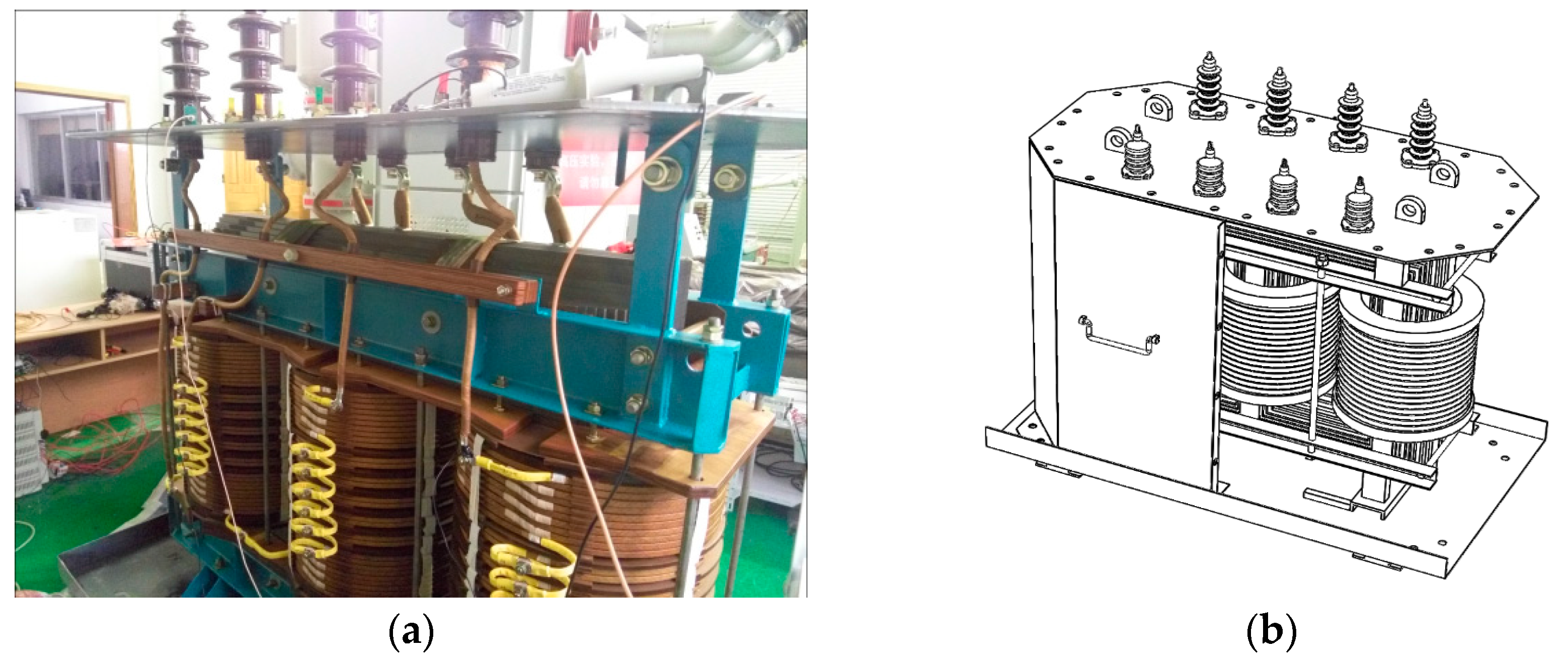
In this paper, we have established a test platform for simulating the real winding deformation faults, a specially manufactured model transformer is adopted to perform all experiments. The model transformer is a three-phase core type transformer with a voltage ratio of 10/0.4 kV and a rated power of 400 kVA. The vector group of winding is YNyn0 and the rated frequency is 50 Hz. Particularly, the internal configuration of the model transformer is designed as that of a 110 kV power transformer, as shown in Figure 2. The HV winding is designed as the disk type with a numbers of 30 disks, the upper and lower 10-disk windings are an interleaved twist, while the middle 10 disks are a sequential twist. The LV winding is designed as the layer type with 6 layers. The transformer manufacturer also produced some windings with variable deformations, which are used to replace the middle 10-disk windings to simulate the winding radial deformation (RD) faults. Despite the fact that the RD windings are not the windings in which the deformation is directly produced in the replaced healthy winding, there is a difference between RD windings and the healthy windings. However, the effect of RD is much more significant than that of the difference between the windings. The changing trend of the FRA signature of simulated RD windings is similar to the actual RD cases [23]. Thus, it is meaningful to simulate RD by replacing the healthy winding with a new artificially manufactured RD winding.
Three typical winding mechanical deformation fault types including winding RD, inter-disk short circuit (SC), fault and disk space variation (DSV) fault are simulated, in which the healthy windings are replaced or set up.
An inter-disk SC fault is realized by shortening the connectors of the middle sequential twist windings; the more connectors are being shortened, the more the severity of the inter-disk SC fault is emulated.
The image of the winding RD fault is shown in Figure 3. In Figure 3a, d represents the amount of RD which is a variable, θ represents the angle which is fixed at 45°, the ratio of d and the winding radius r are set to be 5%, 7% and 10% to emulate the different degree of RDs produced at one direction. There are also other RD fault windings in which the faults are manufactured at different directions, but the ratio of d and r is fixed at 5%, as shown in Figure 3b.
The DSV fault normally produces the variation of inter-disk capacitance and mutual inductance, however, it has been revealed that the capacitance parameter dominates the effect and this fault could be emulated by changing the inter-disk capacitance parameter [31]. A capacitance is then connected with the connectors of two continuous disks for simulating the DSV fault. The degree of fault is emulated by increasing and decreasing the capacitance value, and the fault location is emulated by changing the sequence numbers of two connectors.
All winding deformation faults were emulated in phase A of the model transformer. In each fault status, following the wiring instruction of Figure 1, 50 groups of the experiment were performed by the detection apparatus with the transformer energized by a three-phase symmetric power source in the HV side. The amplitude of the excitation pulse was 1 kV and the pulse width was 600 ns. The nanosecond pulse was coupled into the transformer winding by CCS, and the response current was measured in the grounded neutral line. The measured 50 groups’ data in the same fault status were averaged to reduce the impact of external noise. The online IFRA signatures in each fault status were then obtained by transforming the time domain signal to the frequency domain, and used for fault diagnosis.
3.2. Experimental Results
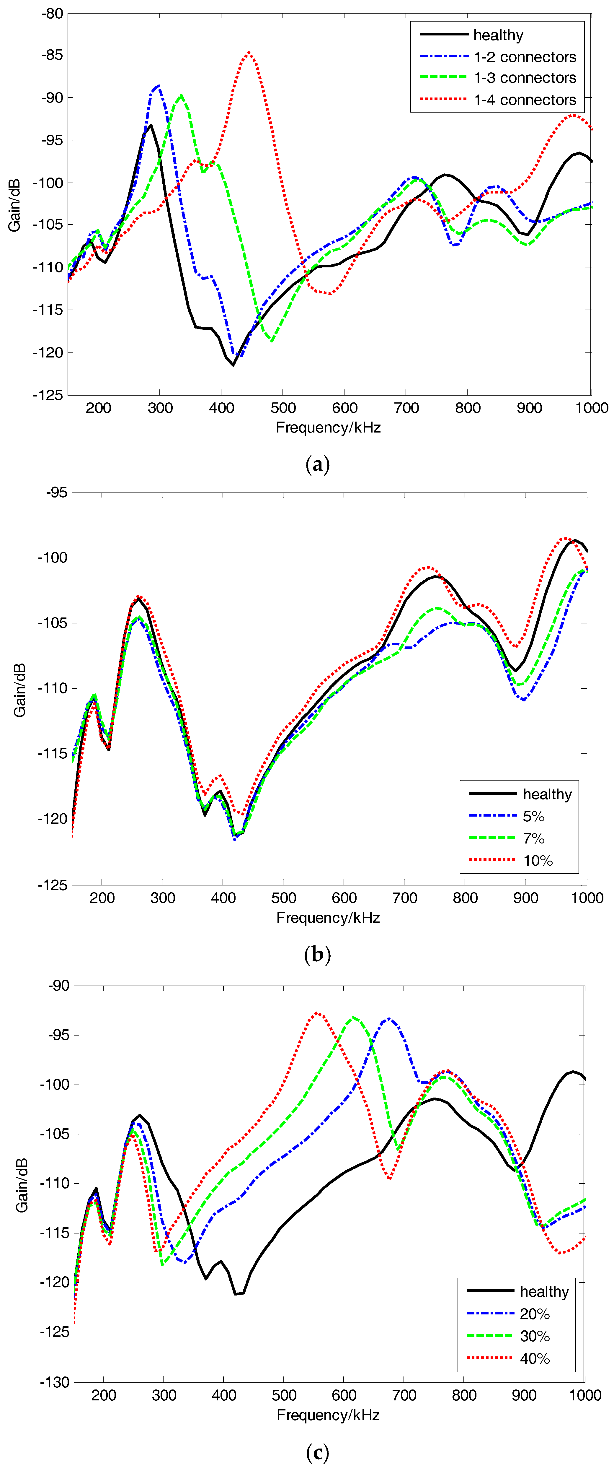
Fifteen groups of inter-disk SC fault were emulated. The detailed experimental setup is shown in Table 1 in which the connector 1~6 represents the connector number of the middle sequential twist windings being seen from top to bottom, as shown in Figure 3a. The IFRA signature under each fault status is obtained with the online IFRA apparatus. Some cases of IFRA signatures under inter-disk SC fault are presented in Figure 4a. It is noted that in reference to [15,20,25] the low frequency band of the online IFRA signature is dominated by the bushing characteristic, and the actual experimental results indicate that the signature in this frequency band is easily disturbed by the external disturbance such as noise, etc., therefore, only the frequency bands of 100–1000 kHz on the signature were analyzed. In the typical cases of Figure 4a, compared with the healthy signature, IFRA signatures of the inter-disk SC fault were different throughout the entire frequency band; additionally, the variation of signatures was much more notable as the fault degree increases.
Considering that the combination of simulated RD status is extensive, the numbers of inter-disk SC fault, 16 groups of winding RD are emulated. The detailed experimental setup is shown in Table 2 in which the position A~E is the location of deformed winding in the middle sequential twist winding, as shown in Figure 3a. Variable deformed disk numbers, fault degree, fault directions and fault locations of RD windings are emulated, and the online IFRA signature in each fault status is obtained. Figure 4b shows some typical cases of online IFRA signatures under simulated RD faults in which all of the middle 10 disks’ healthy windings are replaced by RD fault windings with degrees of 5%, 7% and 10%, all in one direction. It concludes that RD has small impact on the resonant frequency of IFRA signature within 600 kHz, but has induced the variation of resonant frequency in high frequency bands, new resonance and anti-resonance are created around 700 kHz.
Fifteen groups of DSV fault were emulated. The detailed experimental setup is shown in Table 3 in which the connectors 1~4 have the same meaning as those in Table 1, for simulating different fault locations. As for the degree, the numerical value indicates the percentage of the paralleled capacitance to the capacitance of the adjacent healthy disk, in which the capacitance of the adjacent healthy disk is calculated to be approximately 2 nF based on the finite element method. Cases of online IFRA signatures under simulated DSV faults are shown in Figure 4c, in which the degrees of 20%, 30% and 40%, corresponding to the capacitances of 400 pF, 600 pF and 800 pF, are paralleled with the third and fourth connector of the middle sequential twisted disks. Compared with the healthy signature, the faulty IFRA signature changes notably beyond 250 kHz. The signature shifts toward the low frequency band, which shows a significant difference from the effect of inter-disk SC fault. Furthermore, as the fault level increases, the variation of faulty signature becomes more remarkable.
4. Feature Extraction from IFRA Signature
In this paper, we have utilized two indicators extracted from IFRA signatures for fault identification. Winding mechanical deformation normally induces the variation of the IFRA signature, the information of variation should be specially focused and used to interpret the signature. Physically, when an equivalent electrical model of a winding produces series resonance, a peak will be generated in the IFRA signature; when an equivalent electrical model produces parallel resonance, a valley will be generated in the IFRA signature [32]. The resonance and anti-resonance are really matters of the IFRA signature, and the resonant frequency can be a key diagnosis indicator. Statistically, the variation of IFRA signatures is revealed in their shape and trend, all points of the IFRA signature can be calculated. Common statistical indicators for FRA diagnosis range from relative factor (RF), correlation coefficient (CC), area, mean square error (MSE), etc. [33]. The RF and CC represent the similarity degree of two signatures; there might exist a negative number when the difference of two signatures is remarkable, and the minus sign indicates the relevant direction. Nevertheless, MSE reflects the overall difference between the two FRA data, which is always positive numerical; and this positive feature makes MSE suitable for the parameter of intelligent algorithm.
4.1. Indicator of Resonant Frequency Variation
For the indicator of resonant frequency variation (IRFV), the original IFRA data are initially imported into a digital filter for inhibiting the effect of external uncontrollable factors on masking the real resonance and anti-resonance and diminishing the existence of fake resonance and anti-resonance. Particularly, a linear fitting moving average method is adopted to smooth the larger burrs. All resonance and anti-resonance can be extracted and obtained from an IFRA signature by analyzing the neighboring three IFRA points. For example, scanning all IFRA data from the low frequency to the high frequency, if both Xk−1 and Xk+1 are smaller than Xk, Xk should be a resonance; if both Xk−1Xk−1 and Xk+1 are larger than Xk, Xk should be an anti-resonance.
The measured signature and the healthy signature should be compared after extracting all resonant points. The resonant points of the healthy signature (fingerprint) are regarded as bases, and then, the corresponding resonant points of the measured signatures are compared on a case-by-case basis. Each IRFV is obtained based on the following definition and expression. Figure 5 shows three typical situations of resonant point variation in the “frequency domain”, including an offset resonant point, missing resonant point and extra resonant point. Here, the “frequency domain” of the analyzed resonant point, is defined as the frequency range constructed by its neighboring two resonant points in the fingerprint. Figure 5 shows the case of a local maximum resonant point to be analyzed. “Offset resonant point” indicates that there exists one local maximum resonant point on the measured IFRA signature within the “frequency domain”; “missing resonant point” implies that there is no local maximum resonant point on the measured signature within the “frequency domain”; and “extra extreme point” means that there is more than one local maximum resonant point within the “frequency domain”.
For the situation of an offset resonant point, the winding mechanical deformation will generally alter the resonant frequency of the measured IFRA signature, compared to that of the healthy signature. If the measured IFRA signature is offset within the “frequency domain”, the IRFV can be calculated according to Equation (4),
where fk’ and fk are the resonant frequency of k-th resonant point on the measured IFRA signature and the healthy IFRA signature, respectively. IRFVk is the indicator of resonant frequency variation.
For the occurrence of a minor winding deformation, the resonant point of the measured signature will slightly shift; this indicator of offset resonant frequency is typically less than 1 in the analyzed “frequency domain”. However, for the obvious and significant winding deformation, the measured IFRA signature will be missing or extra within the “frequency domain”, and the recommended indicator value can be 1, as shown in Equation (5),
Each IRFV of the measured signature compared with its fingerprint is obtained, a feature vector can be constructed and its dimension is equal to the numbers of resonant points. The vector is then used as the input parameter for the further fault diagnosis and identification based on the advanced machine learning algorithm.
4.2. Indicator of Mean Square Error
For the indicator of mean square error (IMSE), its mathematical expression is defined in Equation (6),
where xi and yi are the gain of the healthy IFRA signature and the measured IFRA signature, respectively, n is the number of the IFRA data in the designated frequency range.
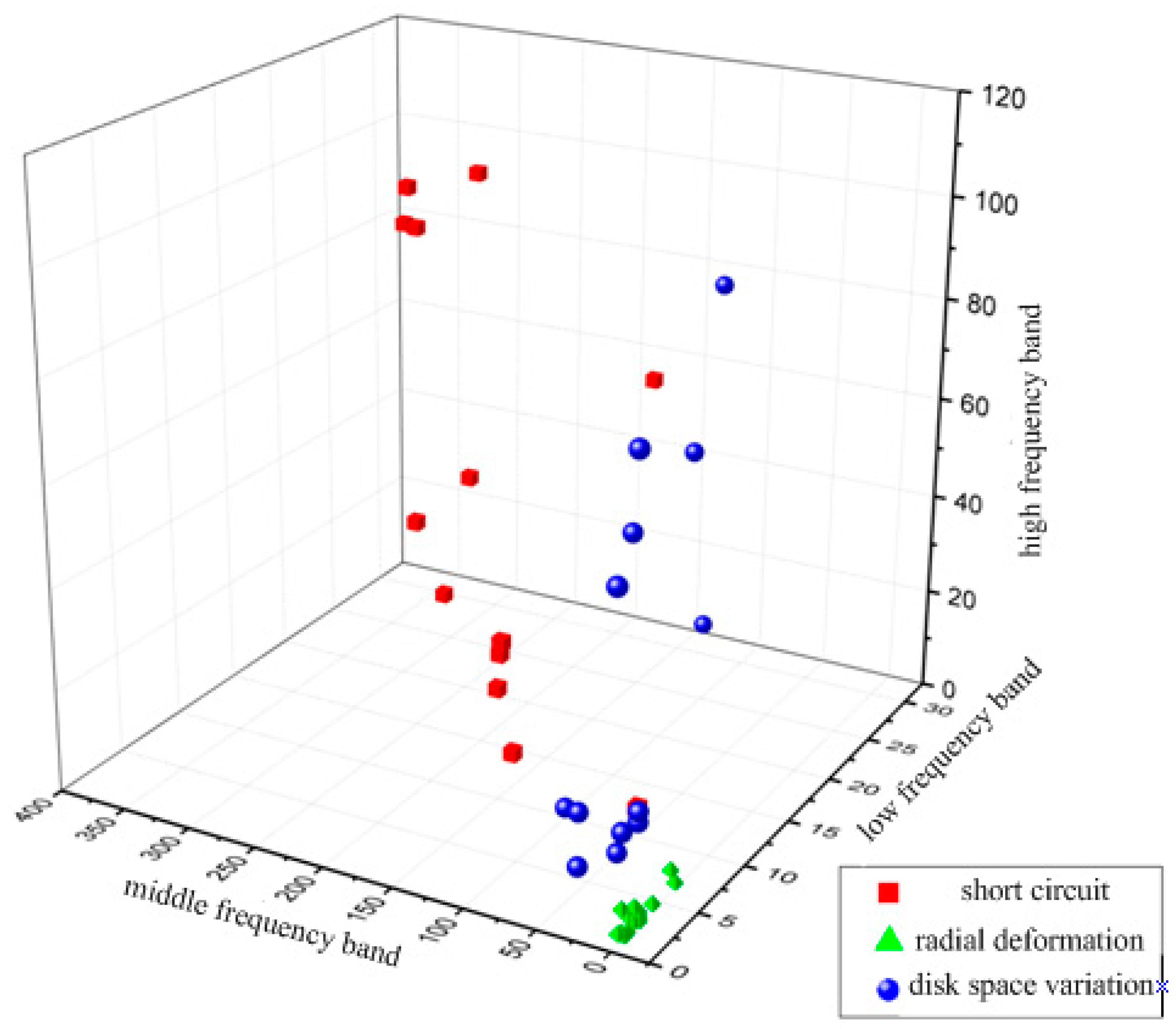
According to the diversity of morphological characteristics for online IFRA signatures in different frequency ranges, the signature can be divided into the low, medium and high frequency band for a more accurate discrimination result. All IFRA signatures, obtained from 46 groups of experiment in Section 3, are processed. For each fault status, the IMSE of healthy and measured signatures in sub-frequency range are calculated, respectively. Namely, the IMSEl, IMSEm and IMSEh are derived. These indicators are plotted in a three-dimensional graph, as shown in Figure 6. The three axis of graph represent the value of IMSEl, IMSEm and IMSEh, respectively. It is concluded from Figure 6 that the distribution of IMSE which corresponds to the RD fault is gathered, while the distributions of IMSE which correspond to the inter-disk SC and DSV fault are dispersed. The reason is that when the interval of fault extent is large for simulating these two types of winding fault. However, the distributions of IMSE for inter-disk SC and DSV in 3D graph are apparently different, and both distributions are different from that of RD. Thus, a vector consisting of IMSEl, IMSEm and IMSEh can be used for fault identification, as shown in Expression (7).
5. Application of Support Vector Machine to Diagnose Winding Fault Types
5.1. Procedure of Identifying Winding Fault Types
SVM has recently been expanded as an emerging machine learning algorithm, which improves the generalization capability of learning machines by seeking the minimum of structural risk, and realizing the minimum of empirical risk and fiducial range. It has particular advantages of solving the classification problem of small-scale samples, non-linearity, and high-dimension. In this paper, the SVM is used for identification of transformer mechanical fault types, wherein the model of fault identification is built by training the sample data.
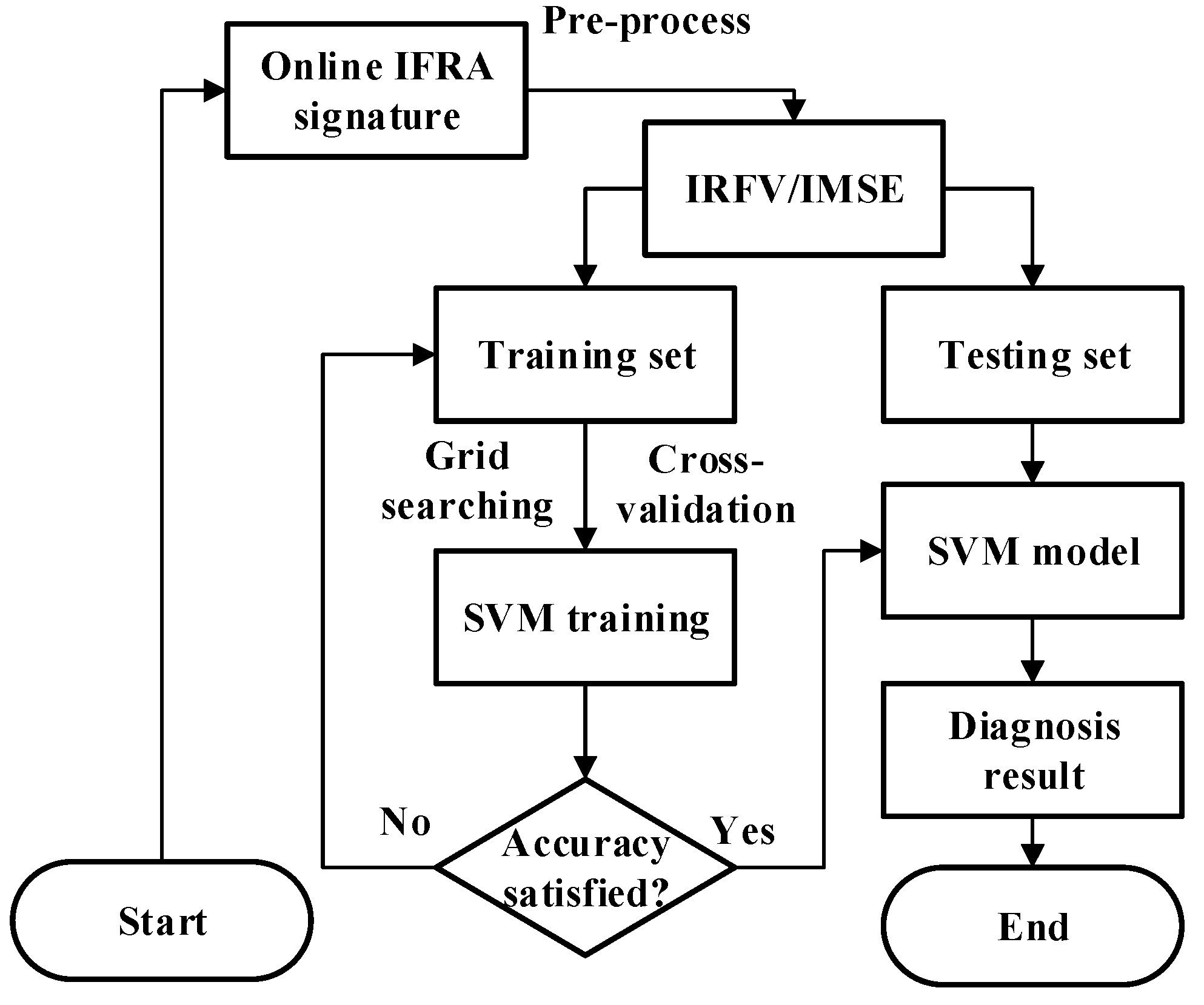
The process of fault identification is shown in Figure 7. As previously described in Section 4, the online IFRA signatures of healthy windings and deformed windings are pre-processed, and the indicators of resonant frequency variation and mean square errors are calculated, respectively. Forty-six groups of testing data are divided into two groups, namely a training set and a testing set. The construction method of two sets is specifically explained in Section 5.2. The training set is adopted to train the SVM model. The training step is constantly continued until the accuracy rate is satisfied, and the SVM model is obtained. The testing set is then input into the SVM model, and the diagnosis result of the winding mechanical fault types is printed out.
For the SVM, the common kernel function includes polynomial, radial basis function (RBF), Sigmoid function and B-Spline, et al. [34]. Vapnik believes that different kernel function has little impact on the performance of SVM [35], the most frequently used RBF has been chosen as the kernel function, and its function is expressed in Equation (8).
The parameter g of RBF and penalty coefficient C of SVM are significant factors to influence the performance of SVM, their initial value are unknown. The grid searching and cross validation algorithm are used to realize the parameter optimization. The grid searching is a trial of various possible (C, g), while in the cross validation, the training set is divided into n parts equally; n − 1 parts of them are regarded as the training data, the rest one part is the testing data. Repeat n times operations, obtain the accuracy rate of SVM identification each time and further calculate the average accuracy rate. The optimized (C, g) corresponds to the highest average accuracy rate among various (C, g).
5.2. Construction of Training Set and Testing Set
For the indicator of the resonant frequency variation, both the training set and testing set are constructed according to Expression (9). In the expression, s represents the inter-disk SC fault, n indicates the number of training set or testing set for short circuit; r represents the RD fault, m indicates the number of training set or testing set for RD; c represents the DSV fault, q indicates the number of training set or testing set for DSV. k is the dimension of feature vector, decided by the numbers of resonant points of healthy IFRA signature. The value of k is 8 for the model transformer. In the training set, both n and q are 10, m equals to 11; the training set is a matrix with 31 rows and eight columns. In the testing set, n, m and q are 5; the testing set is a matrix with 15 rows and eight columns.
For the indicator of mean square error, both the training set and testing set are constructed according to Expression (10). In this expression, s, n, r, m, c and q have the same meaning as those in Expression (9). L represents the low frequency band, M indicates the medium frequency band and H means the high frequency band. In the training set, both n and q are 10, m equals to 11; the training set is a matrix with 31 rows and three columns. In the testing set, n, m and q are five; the testing set is a matrix with 15 rows and three columns. Additionally, for avoiding the interference of human factors on selecting the training set and the testing set, the data of the training set should be selected randomly, and the rest of test sample should form the testing set.
5.3. Diagnostic Result
For the indicator of resonant frequency variation, the diagnostic result of a typical testing set by SVM is shown in Table 4. It can be seen that the diagnostic accuracy rate of the inter-disk SC, RD and DSV is 100%, 80% and 80%, respectively; the average accuracy rate is 86.7%. In addition, a total of 10 groups’ combinations of training and testing sets are randomly constructed from the experimental data, and the identification accuracy rate is shown in Table 5. It concludes that the diagnostic accuracy rate of most groups reaches 75% above, and the overall average accuracy rate is 78.1%, which indicates a satisfied diagnostic result obtained by SVM algorithm.
For the indicator of the mean square error, similarly, the diagnostic result of a typical testing set by SVM is shown in Table 6. Table 6 shows the diagnostic accuracy rate of SC, RD and DSV is 100%, 100% and 80%, respectively; the average accuracy rate is 93.3%. In addition, a total of 10 groups’ combinations of training and testing sets are randomly constructed from the experimental data, and their identification accuracy rate is shown in Table 7. The diagnostic accuracy rate of most groups reaches 80% above, and the overall average accuracy rate is 83.3%, which also demonstrates a satisfied diagnostic result obtained by SVM algorithm.
5.4. Comparison of Two Indicators
The dimension of the feature vector consisting of IRFV depends on the resonant frequency of IFRA signature, for the tested model transformer, the number of resonance and anti-resonance is eight, thus, this dimension is eight However, for the transformer of different rating and capacity, the IFRA signatures are dependent of transformer parameters and obviously different from each other. Although the IRFV indicator includes the detailed information of transformer winding, the dimension of IRFV feature vector can be variable, which increases the complexity of identification by SVM. Further modification should be applied to improve the generalization performance of IRFV indicator.
Additionally, the dimension of the feature vector consisting of IMSE is fixed at three for different transformers; the trained SVM model can be easily upgraded by adding the new frequency response data of other transformers. Although the indicator of resonant frequency variation contains more information, the indicator of mean square error seems more suitable for identifying and classifying the actual transformer internal mechanical faults.
6. Conclusions and Future Work
This paper utilizes the highly intelligent SVM to identity the fault types of transformer winding mechanical deformations. To validate the proposed method by real transformer fault data, a test bed that includes a specially manufactured model transformer is proposed to simulate the winding deformation faults, including the inter-disk SC fault, RD and DSV. 46 groups of online IFRA signatures are obtained with the model transformer energized, the shape characteristic and variation pattern of typical IFRA signatures are analyzed in each faulty circumstance.
Two indicators that separately correspond to the physical essence and data statistics are introduced for constructing the feature vector, including the indicator of resonant frequency variation and the indicator of mean square error. The indicator of resonant frequency variation is calculated in the defined “frequency domain”, while the distribution characteristic of the mean square error in sub-frequency band is presented in the three dimensional space to obtain the feature vector.
Finally, the case study of SVM algorithm for identification is presented. The training set and testing set are randomly chosen from the sample data. For the indicator of resonant frequency variation, the average accuracy rate of ten groups’ testing sets is 78.1%, while for the indicator of mean square error; the average accuracy rate reaches 83.3%, which shows satisfied classifying result for both methods. Further explanation indicates the advantage of the second feature vector by simply upgrading the SVM model with the new added transformer data, which is more suitable for diagnosis of actual power transformer faults. Future work is the necessity for further investigation on classifying the extent and location of the winding mechanical deformations.
Acknowledgments
This work was supported by the Fundamental Research Funds for the Central Universities (Doctoral startup fund in Southwest University), and National Key Research and Development Plan (2017YFB0902702).
Author Contributions
Zhongyong Zhao and Chao Tang conceived and designed the experiments. Qu Zhou and Yingang Gui performed the experiments. Lingna Xu designed the algorithms. Chenguo Yao did the evaluations. All of the authors participated in the project, and they read and approved the final manuscript.
Conflicts of Interest
The authors declare no conflict of interest.
References
- Lee, B.; Park, J.-W.; Crossley, P.; Kang, Y. Induced Voltages Ratio-Based Algorithm for Fault Detection, and Faulted Phase and Winding Identification of a Three-Winding Power Transformer. Energies 2014, 7, 6031–6049. [Google Scholar] [CrossRef]
- Ebrahimi, B.M.; Saffari, S.; Faiz, J.; Fereidunian, A. Analytical estimation of short circuit axial and radial forces on power transformers windings. IET Gener. Transm. Distrib. 2014, 8, 250–260. [Google Scholar] [CrossRef]
- Abu-Siada, A.; Islam, S. A novel online technique to detect power transformer winding faults. IEEE Trans. Power Deliv. 2012, 27, 849–857. [Google Scholar]
- Bagheri, M.; Naderi, M.S.; Blackburn, T. Advanced transformer winding deformation diagnosis: Moving from off-line to on-line. IEEE Trans. Dielectr. Electr. Insul. 2012, 19. [Google Scholar] [CrossRef]
- Ji, T.Y.; Tang, W.H.; Wu, Q.H. Detection of power transformer winding deformation and variation of measurement connections using a hybrid winding model. Electr. Power Syst. Res. 2012, 87, 39–46. [Google Scholar] [CrossRef]
- Hejazi, M.A.; Gharehpetian, G.B.; Moradi, G.; Alehosseini, H.A.; Mohammadi, M. Online monitoring of transformer winding axial displacement and its extent using scattering parameters and k-nearest neighbour method. IET Gener. Transm. Distrib. 2011, 5, 824. [Google Scholar] [CrossRef]
- Dick, E.; Erven, C. Transformer diagnostic testing by frequuency response analysis. IEEE Trans. Power Appar. Syst. 1978, 6, 2144–2153. [Google Scholar] [CrossRef]
- Bagheri, M.; Naderi, M.S.; Blackburn, T.; Phung, T. Frequency response analysis and short-circuit impedance measurement in detection of winding deformation within power transformers. IEEE Electr. Insul. Mag. 2013, 29, 33–40. [Google Scholar] [CrossRef]
- Portilla, W.H.; Mayor, G.A.; Guerra, J.P.; Gonzalez-Garcia, C. Detection of transformer faults using frequency-response traces in the low-frequency bandwidth. IEEE Trans. Ind. Electron. 2014, 61, 4971–4978. [Google Scholar]
- Alsuhaibani, S.; Khan, Y.; Beroual, A.; Malik, N. A Review of Frequency Response Analysis Methods for Power Transformer Diagnostics. Energies 2016, 9, 879. [Google Scholar]
- Leibfried, T.; Feser, K. Monitoring of power transformers using the transfer function method. IEEE Trans. Power Deliv. 1999, 14, 1333–1341. [Google Scholar] [CrossRef]
- Lavrinovich, V.A.; Mytnikov, A.V. Development of pulsed method for diagnostics of transformer windings based on short probe impulse. IEEE Trans. Dielectr. Electr. Insul. 2015, 22, 2041–2045. [Google Scholar] [CrossRef]
- Behjat, V.; Vahedi, A.; Setayeshmehr, A.; Borsi, H.; Gockenbach, E. Sweep frequency response analysis for diagnosis of low level short circuit faults on the windings of power transformers: An experimental study. Int. J. Electr. Power Energy Syst. 2012, 42, 78–90. [Google Scholar] [CrossRef]
- Behjat, V.; Vahedi, A.; Setayeshmehr, A.; Borsi, H.; Gockenbach, E. Diagnosing shorted turns on the windings of power transformers based upon online FRA using capacitive and inductive couplings. IEEE Trans. Power Deliv. 2011, 26, 2123–2133. [Google Scholar] [CrossRef]
- Bagheri, M.; Naderi, M.S.; Blackburn, T.; Phung, B. Bushing characteristic impacts on on-line frequency response analysis of transformer winding. In Proceedings of the 2012 IEEE International Conference on Power and Energy (PECon), Kota Kinabalu, Malaysia, 2–5 December 2012; pp. 956–961. [Google Scholar]
- Leibfried, T.; Feser, K. On-line monitoring of transformers by means of the transfer function method. In Proceedings of the Conference Record of the 1994 IEEE International Symposium on Electrical Insulation, Pittsburgh, PA, USA, 5–8 June 1994; pp. 111–114. [Google Scholar]
- Wang, M. Winding Movement and Condition Monitoring of Power Transformers in Service; University of British Columbia: Vancouver, BC, Canada, 2003. [Google Scholar]
- De Rybel, T.; Singh, A.; Vandermaar, J.A.; Wang, M.; Marti, J.R.; Srivastava, K. Apparatus for online power transformer winding monitoring using bushing tap injection. IEEE Trans. Power Deliv. 2009, 24, 996–1003. [Google Scholar] [CrossRef]
- Yao, C.; Zhao, Z.; Chen, Y.; Zhao, X.; Li, Z.; Wang, Y.; Zhou, Z.; Wei, G. Transformer winding deformation diagnostic system using online high frequency signal injection by capacitive coupling. IEEE Trans. Dielectr. Electr. Insul. 2014, 21, 1486–1492. [Google Scholar] [CrossRef]
- Zhao, Z.; Yao, C.; Zhao, X.; Hashemnia, N.; Islam, S. Impact of capacitive coupling circuit on online impulse frequency response of a power transformer. IEEE Trans. Dielectr. Electr. Insul. 2016, 23, 1285–1293. [Google Scholar] [CrossRef]
- Hashemnia, N.; Abu-Siada, A.; Islam, S. Improved power transformer winding fault detection using FRA diagnostics—Part 1: Axial displacement simulation. IEEE Trans. Dielectr. Electr. Insul. 2015, 22, 556–563. [Google Scholar] [CrossRef]
- Saleh, S.M.; El-Hoshy, S.H.; Gouda, O.E. Proposed diagnostic methodology using the cross-correlation coefficient factor technique for power transformer fault identification. IET Electr. Power Appl. 2017, 11, 412–422. [Google Scholar] [CrossRef]
- Rahimpour, E.; Jabbari, M.; Tenbohlen, S. Mathematical comparison methods to assess transfer functions of transformers to detect different types of mechanical faults. IEEE Trans. Power Deliv. 2010, 25, 2544–2555. [Google Scholar] [CrossRef]
- Bigdeli, M.; Vakilian, M.; Rahimpour, E. Transformer winding faults classification based on transfer function analysis by support vector machine. IET Electr. Power Appl. 2012, 6, 268–276. [Google Scholar] [CrossRef]
- Bagheri, M.; Nezhivenko, S.; Phung, B. Loss of low-frequency data in on-line frequency response analysis of transformers. IEEE Electr. Insul. Mag. 2017, 33, 32–39. [Google Scholar] [CrossRef]
- Li, C.; Xia, Q.; Zhao, Z.; Yao, C.; Mi, Y.; Zhao, X.; Wang, J. Impact analysis of the capacitive coupling sensor on bushing external insulation. IET Gener. Transm. Distrib. 2016, 10, 3663–3670. [Google Scholar] [CrossRef]
- Yao, C.; Zhao, Z.; Li, C.; Chen, X.; Zhao, Y.; Zhao, X.; Wang, J.; Li, W. Noninvasive method for online detection of internal winding faults of 750 kV EHV shunt reactors. IEEE Trans. Dielectr. Electr. Insul. 2015, 22, 2833–2840. [Google Scholar] [CrossRef]
- Gomez-Luna, E.; Mayor, G.A.; Gonzalez-Garcia, C.; Guerra, J.P. Current status and future trends in frequency-response analysis with a transformer in service. IEEE Trans. Power Deliv. 2013, 28, 1024–1031. [Google Scholar] [CrossRef]
- Tenbohlen, S.; Coenen, S.; Djamali, M.; Müller, A.; Samimi, M.; Siegel, M. Diagnostic Measurements for Power Transformers. Energies 2016, 9, 347. [Google Scholar] [CrossRef]
- Yang, Q.; Su, P.; Chen, Y. Comparison of Impulse Wave and Sweep Frequency Response Analysis Methods for Diagnosis of Transformer Winding Faults. Energies 2017, 10, 431. [Google Scholar] [CrossRef]
- Abu-Siada, A.; Hashemnia, N.; Islam, S.; Masoum, M.A. Understanding power transformer frequency response analysis signatures. IEEE Electr. Insul. Mag. 2013, 29, 48–56. [Google Scholar] [CrossRef]
- Wang, Z.; Li, J.; Sofian, D.M. Interpretation of transformer FRA responses—Part I: Influence of winding structure. IEEE Trans. Power Deliv. 2009, 24, 703–710. [Google Scholar] [CrossRef]
- Samimi, M.H.; Tenbohlen, S. FRA interpretation using numerical indices: State-of-the-art. Int. J. Electr. Power Energy Syst. 2017, 89, 115–125. [Google Scholar] [CrossRef]
- Cherkassky, V.; Ma, Y. Practical selection of SVM parameters and noise estimation for SVM regression. Neural Netw. 2004, 17, 113–126. [Google Scholar] [CrossRef]
- Cortes, C.; Vapnik, V. Support-vector networks. Mach. Learn. 1995, 20, 273–297. [Google Scholar] [CrossRef]
Figure 1.
Wring of the online impulse frequency response analysis (IFRA) method applied in a running transformer.
Figure 1.
Wring of the online impulse frequency response analysis (IFRA) method applied in a running transformer.

Figure 2.
Tested model transformer: (a) image of model transformer; (b) 3D diagrammatic sketch of model transformer.
Figure 2.
Tested model transformer: (a) image of model transformer; (b) 3D diagrammatic sketch of model transformer.

Figure 3.
Diagrammatic sketch of winding radial deformation (RD): (a) diagram and image of RD; (b) 3D visualization of winding RD with faults manufactured at different directions.
Figure 3.
Diagrammatic sketch of winding radial deformation (RD): (a) diagram and image of RD; (b) 3D visualization of winding RD with faults manufactured at different directions.

Figure 4.
Some cases of experimental IFRA signatures under different simulated winding deformation faults: (a) simulated inter-disk SC fault; (b) simulated RD fault; (c) simulated DSV fault.
Figure 4.
Some cases of experimental IFRA signatures under different simulated winding deformation faults: (a) simulated inter-disk SC fault; (b) simulated RD fault; (c) simulated DSV fault.

Figure 5.
Three typical situations of resonant point variation.

Figure 6.
Distribution of mean square error of IFRA signatures under various winding faults.

Figure 7.
Process of fault diagnosis by support vector machine (SVM).


Table 1.
Setup of inter-disk short circuit (SC) fault in middle 10-disk windings.
| No. | Connector | No. | Connector |
|---|---|---|---|
| 1 | 1-2 | 9 | 2-6 |
| 2 | 1-3 | 10 | 3-4 |
| 3 | 1-4 | 11 | 3-5 |
| 4 | 1-5 | 12 | 3-6 |
| 5 | 1-6 | 13 | 4-5 |
| 6 | 2-3 | 14 | 4-6 |
| 7 | 2-4 | 15 | 5-6 |
| 8 | 2-5 |
Table 2.
Setup of RD fault in middle 10-disk windings.
| No. | Disk Numbers | Degree | Direction | Location |
|---|---|---|---|---|
| 1 | 2 | 5% | 1 | A |
| 2 | 2 | 7% | 1 | A |
| 3 | 2 | 10% | 1 | A |
| 4 | 2 | 5% | 2 | A |
| 5 | 2 | 5% | 3 | A |
| 6 | 2 | 5% | 4 | A |
| 7 | 10 | 5% | 1 | A~E |
| 8 | 10 | 7% | 1 | A~E |
| 9 | 10 | 10% | 1 | A~E |
| 10 | 10 | 5% | 2 | A~E |
| 11 | 10 | 5% | 3 | A~E |
| 12 | 10 | 5% | 4 | A~E |
| 13 | 2 | 10% | 1 | B |
| 14 | 2 | 10% | 1 | C |
| 15 | 2 | 10% | 1 | D |
| 16 | 2 | 10% | 1 | E |
Table 3.
Setup of disc space variation (DSV) fault in middle 10-disk windings.
| No. | Connector | Degree | No. | Connector | Degree |
|---|---|---|---|---|---|
| 1 | 1-2 | 5% | 9 | 2-3 | 30% |
| 2 | 1-2 | 10% | 10 | 2-3 | 40% |
| 3 | 1-2 | 20% | 11 | 3-4 | 5% |
| 4 | 1-2 | 30% | 12 | 3-4 | 10% |
| 5 | 1-2 | 40% | 13 | 3-4 | 20% |
| 6 | 2-3 | 5% | 14 | 3-4 | 30% |
| 7 | 2-3 | 10% | 15 | 3-4 | 40% |
| 8 | 2-3 | 20% |
Table 4.
Result of classifying a typical testing set using SVM (IRFV).
| No. | Fault Types | Diagnostic Result | Diagnostic Accuracy Rate |
|---|---|---|---|
| 1 | SC | SC | 100% |
| 2 | SC | SC | |
| 3 | SC | SC | |
| 4 | SC | SC | |
| 5 | SC | SC | |
| 6 | RD | RD | 80% |
| 7 | RD | RD | |
| 8 | RD | DSV | |
| 9 | RD | RD | |
| 10 | RD | RD | |
| 11 | DSV | DSV | 80% |
| 12 | DSV | DSV | |
| 13 | DSV | SC | |
| 14 | DSV | DSV | |
| 15 | DSV | DSV | |
| Average accuracy rate | 86.7% | ||
Table 5.
Identification accuracy rate of 10 groups’ randomly chosen testing sets (IRFV).
| No. | Diagnostic Accuracy Rate |
|---|---|
| 1 | 73.3% |
| 2 | 66.7% |
| 3 | 80.0% |
| 4 | 77.3% |
| 5 | 86.7% |
| 6 | 77.3% |
| 7 | 73.3% |
| 8 | 80.0% |
| 9 | 80.0% |
| 10 | 86.7% |
| Average | 78.1% |
Table 6.
Result of classifying a typical testing set using SVM (IMSE).
| No. | Fault Types | Diagnostic Result | Diagnostic Accuracy Rate |
|---|---|---|---|
| 1 | SC | SC | 100% |
| 2 | SC | SC | |
| 3 | SC | SC | |
| 4 | SC | SC | |
| 5 | SC | SC | |
| 6 | RD | RD | 100% |
| 7 | RD | RD | |
| 8 | RD | RD | |
| 9 | RD | RD | |
| 10 | RD | RD | |
| 11 | DSV | DSV | 80% |
| 12 | DSV | DSV | |
| 13 | DSV | RD | |
| 14 | DSV | DSV | |
| 15 | DSV | DSV | |
| Average accuracy rate | 93.3% | ||
Table 7.
Identification accuracy rate of 10 groups’ randomly chosen testing sets (IMSE).
| No. | Diagnostic Accuracy Rate |
|---|---|
| 1 | 100.0% |
| 2 | 73.3% |
| 3 | 93.3% |
| 4 | 80.0% |
| 5 | 86.7% |
| 6 | 80.0% |
| 7 | 80.0% |
| 8 | 86.7% |
| 9 | 73.3% |
| 10 | 80.0% |
| Average | 83.3% |
© 2017 by the authors. Licensee MDPI, Basel, Switzerland. This article is an open access article distributed under the terms and conditions of the Creative Commons Attribution (CC BY) license (http://creativecommons.org/licenses/by/4.0/).
Share and Cite
MDPI and ACS Style
Zhao, Z.; Tang, C.; Zhou, Q.; Xu, L.; Gui, Y.; Yao, C. Identification of Power Transformer Winding Mechanical Fault Types Based on Online IFRA by Support Vector Machine. Energies 2017, 10, 2022. https://doi.org/10.3390/en10122022
AMA Style
Zhao Z, Tang C, Zhou Q, Xu L, Gui Y, Yao C. Identification of Power Transformer Winding Mechanical Fault Types Based on Online IFRA by Support Vector Machine. Energies. 2017; 10(12):2022. https://doi.org/10.3390/en10122022
Chicago/Turabian StyleZhao, Zhongyong, Chao Tang, Qu Zhou, Lingna Xu, Yingang Gui, and Chenguo Yao. 2017. "Identification of Power Transformer Winding Mechanical Fault Types Based on Online IFRA by Support Vector Machine" Energies 10, no. 12: 2022. https://doi.org/10.3390/en10122022
Note that from the first issue of 2016, this journal uses article numbers instead of page numbers. See further details here.