The Rebound Effect of Energy Efficiency Policy in the Presence of Energy Theft


1
Department of Economics, Iowa State University, Ames, IA 50011, USA
2
Department of Economics, Istanbul Technical University, Istanbul 34467, Turkey
*
Author to whom correspondence should be addressed.
Energies 2018, 11(12), 3379; https://doi.org/10.3390/en11123379
Submission received: 16 October 2018
/
Revised: 5 November 2018
/
Accepted: 13 November 2018
/
Published: 3 December 2018
(This article belongs to the Special Issue Energy Policy and Policy Implications)
Abstract
:Introduction: Estimating the effectiveness of energy efficiency policy in reducing energy use requires a full understanding of the energy efficiency rebound effect, where energy use reductions differ from engineering expectations. Prior models that estimate the size of the total rebound effect ignore energy theft, which is a common feature in developing economies. Objectives: The primary objective of this study was to evaluate the role that energy theft plays in determination of the size of the rebound effect of energy efficiency policy in developing countries, using the Turkish economy and the specific Turkish regulation regarding compensation for energy theft as an example. Methods: We construct two energy-economy computable general equilibrium (CGE) models for Turkey that do and do not incorporate energy theft. Costs of energy theft are passed on to consumers through a recovery surcharge. Two energy efficiency policies are modeled; one leading to a 42% energy efficiency increment for the service sector and another leading to a 48% energy efficiency increment for households. Results: Without energy theft, rebound effects for both policies are small: between −1.4% and 3.1% for the service sector and between 0.4% and 2.1% for households. With energy theft, we see a −7.9% to −19.7% rebound for the service sector and a 10.4% to 40.7% rebound for households. The recovery surcharge on energy sales rises when energy efficiency gains affect the service sector but fall when they affect households. Conclusions: The interaction between energy efficiency and energy theft may be critical in accurate estimation of rebound effects where energy theft is prevalent. Where energy efficiency gains disproportionately reduce electricity sales rather than theft, the rising recovery surcharge leads to a negative rebound or super-conservation. However, where theft is disproportionately reduced rebound will be higher.
1. Introduction
Energy efficiency is important for reducing resource use and emissions. However, in the literature there is an ongoing debate about offsetting impacts called “take-back effects” or “rebound effects”. According to economic theory, an increase in energy efficiency may reduce the per unit price of energy services. The cost of these services is a combination of the purchase price of goods and of the energy used to power them. The energy service cost reduction stimulates energy demand from both consumers and firms. In addition, if there is an energy price reduction this may also lead to changes in demand for other goods energy. The first effect is referred to as a direct rebound and the second an indirect or secondary rebound effect [1]. Changes in relative prices as well as increased or reallocated income will also cause non-direct rebound effects. In this study we examine total or economy-wide rebound effects, consisting of the sum of direct and indirect or secondary effects [1]. Among studies which estimate total rebound effects, there is consistency in what is and is not considered to be a direct rebound effect and the sources of total rebound which differ from direct rebound. However, studies differ in rebound typology with some, such as Greening et al. [2] and Barker et al. [3], that classify rebound into direct, indirect/secondary and economy-wide with total rebound being the sum of the three. For typology, we follow Sorrell [1] with total and economy-wide rebound treated as synonymous with all non-direct rebound classified as indirect.
A substantial literature exists that estimates the magnitude of the rebound effect in a variety of different national and sectoral contexts. However, these studies ignore the phenomenon of energy theft, which may be common in developing countries, and as a result may draw conclusions that are accurate only for developed countries where energy theft is rare for energy efficiency policies in one such developing country—Turkey—in order to analyze the important role of energy theft in rebound estimation. To our knowledge, no rebound study has previously been conducted incorporating energy theft nor for Turkey and this paper aims to fill these gaps in the literature.
In the case of Turkey energy efficiency is a crucial policy issue; as Turkey imports most of its primary energy resources. Turkey wants to reduce energy and fuel imports while maintaining economic growth. In addition to economic concerns, after signing the Kyoto Protocol in 2004 growth in Turkish energy consumption should controlled in order to reduce future greenhouse gas emissions. Turkey has several policies that aim to promote energy efficiency. By 2020 the expected increment in overall efficiency is 15% due to policy according to the International Energy Agency’s (IEA) 2009 Turkey report [4]. As a result, estimation of the effect of these policies on actual energy use is politically relevant for Turkey. From a global perspective, Turkey makes up a small proportion of global energy consumption, however dynamics of energy use in Turkey may be similar to a broad class of developing countries. Conclusions drawn regarding the effects of Turkish policy may be important for researchers and policy makers in these countries, which have similar features.
The features common to developing countries that the Turkish economy has may impact the presence or size of rebound effects observed from different types of energy efficiency improvements. Turkey has a substantial informal or shadow economy; sectors which produce similar goods to formal sectors while avoiding official recognition, regulation and tax payments. Shadow sectors in Turkey and globally tend to pay low wages to informal workers and to have low labor productivity. Turkey also experiences the routine theft of energy from the grid by both households and firms [5]. This is most common in Turkey’s economically underdeveloped southeast, but accounts for a non-trivial portion of total energy consumption in other regions as well. Electricity distributors lack the technical or institutional capability to identify and punish thieves individually and instead pass on costs equally to all paying customers. Firms and consumers who ignore regulation, or who do not pay for the electricity they consume may have different reactions to changes in energy efficiency than others [5]. To our knowledge no previous analysis of rebound effects has attempted to incorporate these features and to examine the effect of energy theft on estimates of the size of the rebound effect. As a result, prior models which estimate economy-wide rebound may give accurate estimates in developed countries where energy theft is rare but not in developing countries where energy theft is common.
Many studies have been conducted, which give conceptual examples of rebound as well as empirical or simulation-based estimates of the size of that rebound. Usage of fuel efficient cars gives a classic example of the rebound effect in that purchase of a fuel efficient car can cause buyers’ driving habits to change. Since fuel efficiency reduces the marginal cost of driving one more kilometer, the utilization rate of the car can increase. This effect might partially or even fully offset the reduction in energy consumption per kilometer driven on total energy consumption. Another possibility would be that the consumer does not alter her driving habits and simply spends less on fuel. With the money saved she could buy a plane ticket or consume another good and energy may be used in the creation or consumption of that good as well. As her non-automotive energy consumption is greater with a more fuel efficient than with a less fuel efficient car an indirect rebound occurs.
In addition to transportation there are several common examples of direct rebound effects related to individual “energy services” such as; heating, lighting, refrigeration and installation of insulation. For example, consumers may install efficient Light Emitting Diode (LED) light bulbs in their homes in order to reduce electricity bills. Since LED light bulbs will decrease the operating costs of lights consumers may leave their lights on for longer periods or install brighter lights, leading to rebound. Some object to the assumption of this type of direct rebound, arguing that consumers may have a saturation point for individual energy services. Consumers, for example, might not choose to heat their homes beyond their comfort temperature despite improvements in the efficiency of insulation [6].
The assumption of a saturation point for energy service use yields the conclusion that the size of direct rebound effects should be small. However, Wirl [7] argues that price reductions due to energy improvements may allow more consumers to access that service, particularly in developing countries. Introduction of more efficient home air-conditioners may lead more “marginal consumers” to purchase an air-conditioner for the first time [7]. These marginal consumers create rebound by increasing ownership of air-conditioners, which increases their consumption of the complementary energy service. This case may be similar to that observed in Turkey in which peak summer electricity consumption has increased rapidly due to recent growth in the number of air-conditioners.
The impact of improved energy efficiency has long been a controversial issue. First stated in Jevons’ classical work “The coal question” from 1865 [8] it regained attention following the oil crises of the 1970s after which energy efficiency was considered as a potential solution for energy shortages. Khazzoom [9] however proposed that engineering-based calculations of energy consumption due to energy efficiency improvements overlook the fact that energy consumption decisions also have a price component. The assumption that an increase in efficiency of 1 percent would decrease consumption by a full 1 percent was not realizable due to this “rebound effect”.
Rebound can be seen as having 3 different proximate causes or any combination of these: an increase in the utilization rate of the appliance, an increase in the stock of that appliance or increase in ownership of other appliances. Using an empirical methodology Khazzoom [9] first applied own price elasticity of demand estimates for household appliances to show that rebound effects exist and reduce energy savings from energy efficiency. While Khazzoom [10,11] and Brookes [12,13] suggest that rebound effects exist and can potentially create a “backfire” where energy consumption rises due to an increase in energy efficiency, Lovins [6] and Schipper and Grubb [14] claim that rebound is negligible and cause only 1–2% of expected reductions in energy consumption.
Lovins [6] makes two arguments; physical saturation points and the inability of a household to distinguish which appliance is responsible for electricity savings. However, with mandatory energy labeling regulations consumers should be able to obtain more information about electricity savings and consumption. Lastly Lovins argues that elasticity, as used by Khazzoom, is not a good metric to apply directly to energy demand. Despite criticism of relying on elasticities to estimate rebound, many studies [2] follow Khazzoom’s approach. It also remains the case that estimates of total rather than direct rebound, such as ours, calibrate rebound measures to approximate a whole-economy elasticity of energy demand with respect to an energy efficiency increment for comparability to Khazzoom and others.
Saunders [15] demonstrated that the rebound effect is consistent with neo-classical growth theory and defines the concept as the Khazzom-Brookes Postulate. Greening, Greene and Difiglio [2] published a survey of the rebound effect literature and pointed out that more empirical study is needed to estimate the true size of rebound. The rebound effect can be classified as direct and indirect [1] and the preferred model for estimation varies according to type. Direct rebound can be estimated through econometric analysis. Greening, Greene and Difiglio [2] provide a review of 75 empirical studies of the direct rebound effect, which examine the impact of improvements in fuel efficiency on a specific energy service rather than on total fuel consumption. The direct rebound effect of efficiency gains in space heating will be between approximately 10–30%, in space cooling 10–40% and in personal transportation 20–50%. Greening et al. conclude that an increase in energy efficiency will result in an overall reduction in energy consumption, the size of rebound is policy relevant but relatively small. However, Dimitropoulos [16] points out that although direct rebound effects are small for most sectors, the same conclusion does not always apply for economy-wide effects or total effects.
In order to estimate total or economy-wide (sum of direct and indirect) rebound effects, computable general equilibrium (CGE) models are used. Models for countries such as Kenya [17] and China [18] where an energy efficiency improvement has been introduced into production processes show, a backfire with a rebound greater than 100%. However, another recent study [19] for China showed no backfire effects, with a negative rebound for electricity efficiency specifically. Studies for Sudan [20], Sweden ([21] for the 1957 Swedish economy, [22] for an updated version) and Japan [23] show a smaller rebound between 36–77 percent. The model used for Japan is distinguished in how rebound is defined; as the improvement rate of energy efficiency minus reduction rate of carbon dioxide rather than pure energy consumption.
Studies for the UK [24] and Scotland [25] using the same CGE model, with their own national statistics, introduced a 5% rise in energy efficiency in all production sectors. While Scotland faces a backfire in the long run for efficiency improvements in electricity consumption, the UK exhibits only a 14% rebound in the long run for electricity. Another recent study [26] for the UK which considers the same 5% scenario showed that rebound estimates are sensitive to household income, aggregate economic activity and relative prices with a 47.3% short run and 71.6% long run rebound for household energy efficiency. These results illustrate that rebound estimates also depend on the structure of economy and may differ strongly from country to country. Grepperud and Rasmussen [27] point out that the type of energy efficiency change also plays a significant role in determination of the size of rebound. Their model for Norway finds zero rebound for energy efficiency increases in the oil sector but finds a backfire in electricity.
When the global economy is taken as a whole, we can see smaller or larger economy-wide or total rebound effects for a global energy policy depending on model assumptions. Barker et al. [3] analyze a global energy efficiency gain using a global model and find a total rebound effect of 31% in the short run and 52% in the long run. Wei and Liu [28] find that national energy efficiency improvements give a long-run global rebound effect of 70% in the long run due to movements in labor and capital and increases in growth. Koesler et al. [29], using a model of Germany and the rest of the world, find that the global rebound is lower at 46.8% than the national rebound of 50.2% due to a negative leakage effect as the country which experiences an energy efficiency improvement gains a competitive advantage in trade.
Both theoretical and empirical studies reveal that the size of the rebound effect is sensitive to the price elasticity of demand for energy as well as elasticities of substitution between energy and other consumption goods or factors of production; when elasticities are higher a larger rebound is likely to be seen. Saunders [30] illustrates that the selection of functional form for production functions is very important for this reason, with rebound possibilities limited by the choice of form. Certain functional forms do not allow for higher elasticities of substitution in the energy service nest and must therefore result in low estimates of rebound, such forms are frequently used in models applied by the IPCC for example [31]. The strength of the rebound effect for a given sector is strongly influenced by backward and forward linkages to energy or energy-intensive goods, allowing Freire-Gonzalez [32] to construct national indices for vulnerability to rebound based upon input-output coefficients alone. Since these results are difficult to generalize, more empirical study is needed.
As previous studies [15,26] have made clear that a total rebound effect can only be determined using a general equilibrium model that allows for price movements, this is the methodology that we have applied. Our estimation utilizes a nested constant elasticity of substitution (CES) functional form in order to allow for sensitivity analysis with respect to elasticities of substitution with the energy service nest as in Lecca et al. [26]. In order to accurately capture demand responses to energy efficiency in the Turkish context, this study also incorporates energy theft. In the process of production and distribution of energy there may be losses due to both technical and nontechnical reasons. Nontechnical losses can be described as energy theft and consist of fraud (meter tampering), stealing (illegal connections), billing irregularities, and unpaid bills [5]. Distribution companies in Turkey cut off power in case of unpaid bills and billing irregularities therefore energy theft will refer specifically to energy stealing and fraud.
Turkey faces a serious leakage in energy consumption in the form of stealing from the grid; nonpayment, fraud and illegal line connections. While from Dicle Electric Distribution Company in the southeastern region 72% of all electricity is stolen, even Turkey’s largest electricity transmission firm (the Istanbul-area Bogazici Distribution Company) with 4.7 million customers estimates 9.44% electricity theft [33]. This amount of electricity theft has resulted in losses of approximately $1 billion (US) annually [34]. Several studies examine the socio-economic reasons [35], possible governance solutions [36], possible free market solutions [37] as well as the implications of energy theft for possible tariff design [38] in Turkey. This study will focus solely on the implications of existing patterns of theft for energy efficiency rebound.
The problem of energy theft does not seem to be resolvable, at least in the near future, due to the complicated structure of the industry and regulatory institutions as well as political constraints. As a result, the Turkish government has implemented some regulations in order to mitigate the financial burden of energy theft. Privatization of the electricity market and application of a national tariff for electricity prices in which consumers bear the burden of energy theft have been implemented. All 21 transmission companies produce their own loss targets for each year and the Enerji Piyasası Düzenleme Kurumu (EPDK) calculates the total cost of that loss [33]. This cost is then distributed among both residential and commercial customers in the form of a price markup. The burden of electricity theft is represented on electricity bills under a special payment category labelled “illegal usage share”. This share does not differ according to province or consumer type, although theft itself is known to be more prevalent in certain provinces and among certain consumer types. If actual theft is less than that which was targeted, the distribution company keeps the profit and in the opposite case the company incurs a loss. Every year companies renew their target according to actual theft [33]. Within this system certain groups of people and firms exist that do not pay for energy, and their demand will not respond to changes in energy price, nor will an improvement in energy efficiency reduce the cost for them of the associated energy service such as lighting.
The stylized CGE model built for Turkey also incorporates an informal economy. The informal or shadow economy can be defined as all market-based production of goods and services that are deliberately concealed from public authorities. The reasons for this may be payment of income, value added or other taxes, payment of social security contributions, legal labor market standards such as minimum wages, maximum working hours and safety standards or in order to avoid complying with certain administrative procedures that impose a compliance cost [39]. The size of the informal or shadow economy is expressed as a percentage of GDP. While the presence of an informal sector is an undeniable fact the exact size of the informal sector remains ambiguous. In the literature there exist structuralist multi-sector CGE models which incorporate informal sectors for various countries. Gibson and Kelley [40] examine the issue from a theoretical point of view and present generalized findings. Kelley [41] treats formal and informal output as imperfect substitutes and aggregated them into a tradeable composite good (following Armington [42] aggregation). Since the elasticity of substitution between formal and informal output cannot be obtained from literature, Kelley proposed running sensitivity analyses involving different values for this parameter. In his model informal sectors do not pay taxes, do not use imported intermediate goods and do not save.
Gibson [43] provides an additional perspective on Latin American countries using another structuralist CGE model for Paraguay. The informal sector is modeled as explicitly operating alongside the formal sector. Both informal and formal sectors face the same price level where the formal sector determines the price level. In Gibson’s model capital accumulation in informal sectors is driven by savings of the informal sector. Schaefer [44] argues that the characteristics of a country play an important role in determining the elasticity of substitution between formal and informal versions of a good. While informal and formal goods may be substitutes (high elasticity of substitution) for East Asian and Latin American countries this may not be appropriate for African and South Asian countries. In the latter, the informal sector focuses on very low-wage goods and commerce and cannot easily substitute for formal sector output. We treat formal and informal versions of a good as separate goods with independent prices, with a unitary elasticity of substitution between them.
2. Materials and Methods
In order to estimate economy-wide rebound effects we constructed two static neoclassical energy-economy computable general equilibrium (CGE) models for Turkey. Production and utility functions follow the calibrated share, constant elasticity of substitution (CES) functional forms outlined in Rutherford [45,46,47,48] as do model closures (fixed factor endowments and trade balance) and equilibrium conditions (complementary slackness). The models are estimated using GAMS/MPSGE (v.22.1). Our models differ primarily in detail regarding the energy sector and the shadow economy, which are described in some detail below. Construction of the model involved creation of two Social Accounting Matrices or SAMs based on the 2011 Turkey Input-Output table [49] from the World Input Output Database (WIOD) [50]. The SAM is a square or rectangular matrix which shows all transactions within the economy as a circular flow of income and spending [51]. For each agent spending is represented as a column and income is represented as a row. A SAM also includes a financial account composed of national savings and investments as well as government spending and tax payments for each sector. Under an open economy assumption an aggregate rest of the world (ROW) is added to model. ROW spending indicates Turkish exports while ROW income indicates Turkish imports. For each agent, total expenditure must equal total income creating a balanced SAM.
Five industry categories have been aggregated from the WIOD input-output table [50]; agriculture, industry, transportation, service and energy. Each purchases intermediate inputs from other sectors and makes payments to households for the labor and capital that they employ. Wage and capital rental payments provide income to representative households and all taxes are paid to a single government entity. Investments are funded by both household savings and government. Labor supply in Turkey is a fixed endowment, while the capital endowment varies with total investment. Our first model includes only these five industry sectors, as well as capital, government and a single labor type.
To provide a more realistic view of the Turkish economy an informal or shadow economy is included in the SAM used in the second model. The SAM is expanded to nine industries by adding informal agriculture, informal industry, informal transportation and informal service. There is assumed to be no informal energy sector. Formal and informal households supply formal and informal labor respectively. As simplifying assumptions informal sectors pay no tax, hire only informal labor, have lower productivity and make no payments to the energy sector for energy use. Formal sectors pay tax, hire only formal labor, have higher productivity than informal sectors and pay a price for electricity use that includes a markup to cover the cost of electricity stolen by the informal sectors.
Total payments to the single labor group in the first model and SAM by each sector equal the sum of payments by both the formal version of that sector to formal labor and the informal version of that sector to informal labor. Total output by the single version of each sector in the first model and SAM is equal to the sum of the outputs of each version of that sector in the second model and SAM. As the SAM reflects the value of outputs (total expenditure and income), spending on energy by the single version of each sector in the first model and SAM is equal to the spending on energy by the formal version of that sector in the second model and SAM. As a result, the input share of energy by formal sectors in the second model is higher than that of the single version of that sector in the first model. Informal sectors in the second model spend nothing on energy, obtaining it through theft or fraud.
Although the Turkish Statistical Institute (TUIK) does not publish any official record of the informal economy a large literature is available to enable us to model it. Schneider, Buehn and Montenegro [39] contribute a database of the size of and trends in the informal economy in 162 countries over the period 1999 to 2007, giving a 29.1% informal share in Turkey in 2007. Schneider [52] and Schneider and Kearney [53] estimate the share of the informal sector in Turkey as of 2011 to be 27.7% of GDP. Informal employment in Turkey represented 52.1% of total employment in 2002 according to TUİK, decreasing to 40.7% by 2011. The model incorporates 2011 percentages in which 84% of agricultural sector employment is informal whereas in service, transportation and industry sectors this share is 26.6%.
The informal wage rate (and informal sector labor productivity) differs from the formal wage but it is often ambiguous to what extent. Del Bo, Fiorio and Florio [54] provide insight on informal wage rates for EU regions. They classify EU regions into four groups according to their per capita GDP, unemployment rate, rate of long term unemployment, demographic and geographic data including total and active population, rurality and annual net migration flows. The fourth cluster covers countries from Eastern Europe and Greece, many of which are economically similar to Turkey. Shadow wage and conversion factors, the ratio between informal and formal wages, are calculated for each cluster. As expected the shadow wage varies among clusters. The proportionally highest shadow wages are calculated for first cluster with an average conversion factor equal to 1, but only 0.8 and 0.62 respectively, for the second and fourth clusters. The estimated size of the shadow economy in Eastern Europe and Greece is approximately the same as in Turkey [52] and according to World Bank statistics GDP per capita, the unemployment rate and share of agricultural employment in Turkey are similar to fourth cluster countries. Fourth cluster averages from Del Bo, Fiorio and Florio [54] are chosen as a reference point for Turkey. We assume that the informal wage rate and informal labor productivity in Turkey are equal to 62% of the formal wage rate and formal labor productivity.
The informal or shadow economy differs from the formal economy due to its labor market but also in other aspects. According to studies, informal sectors are more labor intensive than their formal counterparts yet the exact capital labor ratio in the informal economy remains uncertain. Accurate data is unavailable for the exact quantity of capital stock used by the informal sector or exact flows of capital income from the informal sector. Cantekin and Elgin [55] examine informality in Turkey and according to their data set, the capital-output ratio in the formal economy is estimated to be three times of that of the of informal economy for Turkey. In construction of reference data for informal sectors in the social accounting matrix for Turkey we have employed the same ratio. In addition, informal sectors do not pay taxes on inputs or outputs and although they consume energy they do not pay for it. It is assumed that informal sectors sell only on the local market and do not export.
The general equilibrium approach views an economy as a closed and interrelated system in which we simultaneously determine the equilibrium values of all variables of interest. Ours is a standard Arrow-Debreu general equilibrium model [56], which solves simultaneously for equilibrium prices and quantities in a system of perfectly competitive markets. Representative firms and households are all small relative to the overall market and as a result are compelled to take market prices as a given. Households and firm managers are rational, firms maximize profits by minimizing costs and consumers maximize utility. This process satisfies an income balance condition, in which firms and households spend (or save/invest) all income received. All markets clear, total supply equals total demand for each sectoral output.
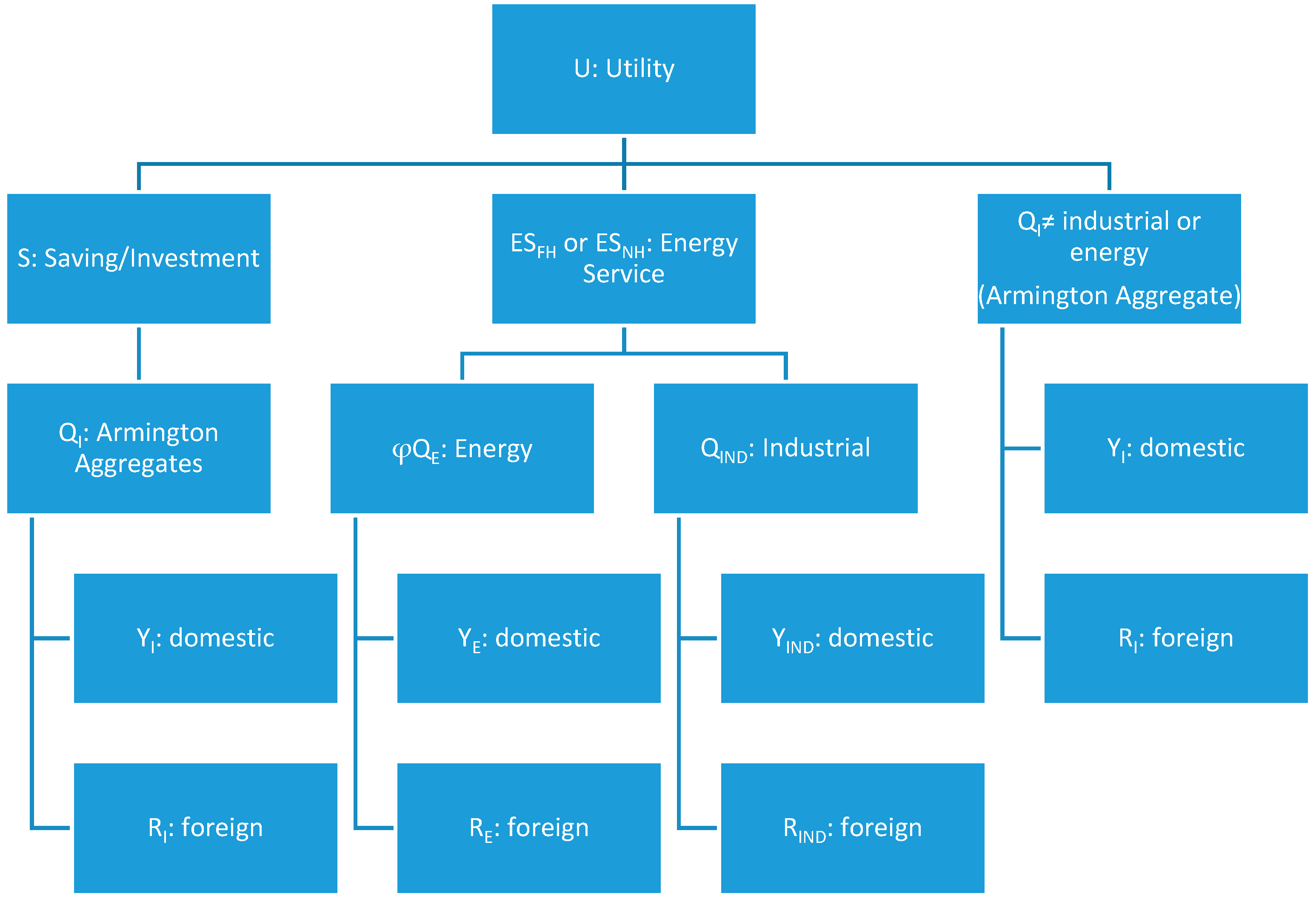
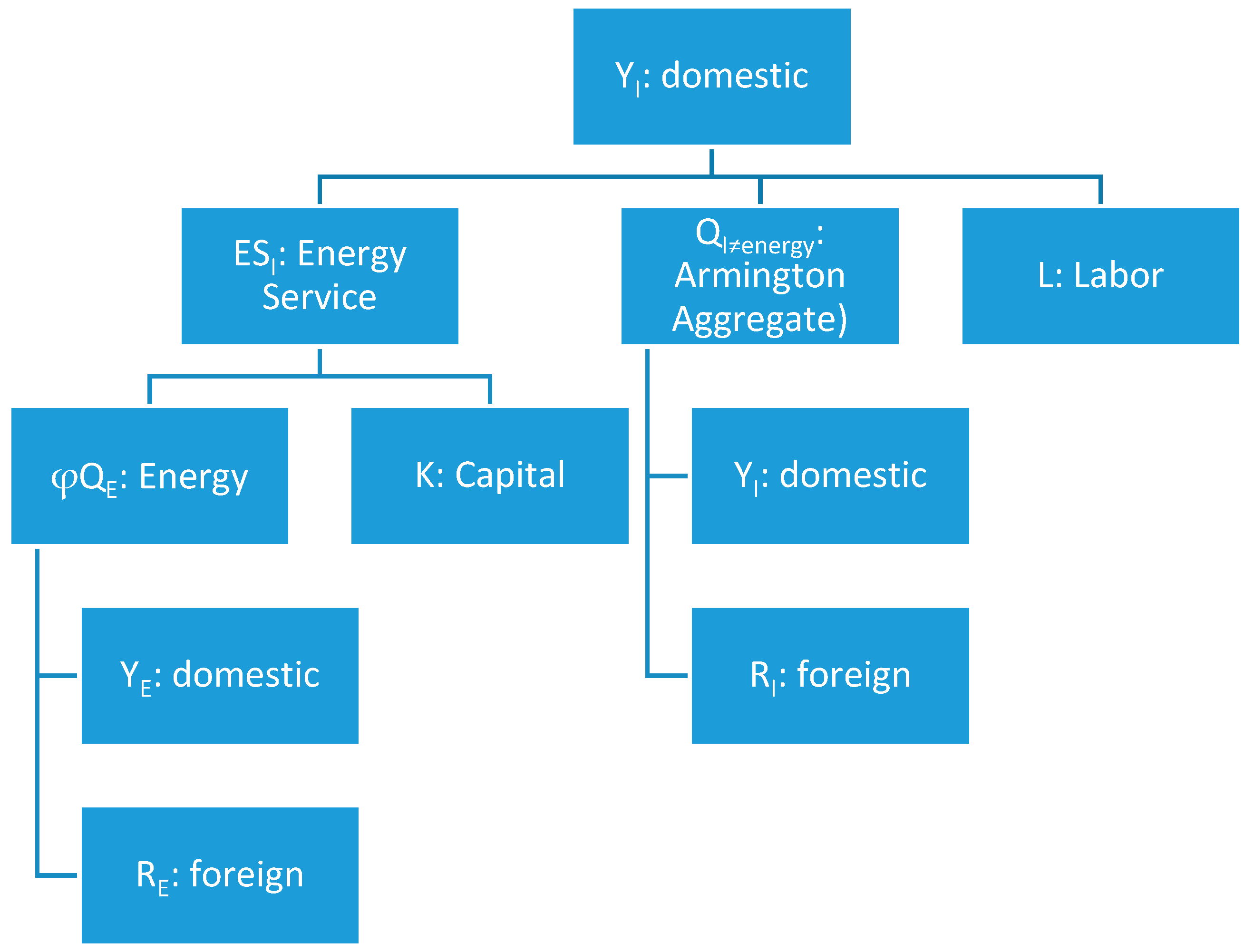
Consumption of goods and services either by households or as intermediates used in production follows an Armington [42] specification. Foreign and domestic versions of all (formal) goods are bundled together, with a unitary elasticity of substitution, before final consumption. Households and firms consume only Armington aggregates of formal sector goods, as well as domestically produced informal sector goods. A detailed description of model equations for the model with energy theft can be found in Appendix A and for the model without energy theft in Appendix B. We use a nested CES structure for production and household utility with a Cobb-Douglas form (unitary elasticity of substitution) at the top level. A nest exists for formal sectors in which energy and capital are treated as complements with a substitution elasticity of 0.5 and a CES structure in generation of the capital-energy bundle [29], an elasticity varied later for sensitivity analysis. The interpretation of this bundle differs by sector; representing building services for the service sector, but powered machinery for agriculture, industry and transportation. Household utility is generated using a Cobb-Douglas functional form from agriculture, services, transportation, savings and an energy service (appliance use) composite created by combining industrial sector goods (both formal and informal) and energy. Industrial goods and energy are treated as complements with an elasticity of substitution of 0.5.
Figure 1 and Figure 2 below display the nesting structure in model production of household utility (Figure 1) and domestic production (Figure 2).
Household utility U is produced using the “here” Armington aggregates Q for non-energy and non-industrial sectors, produced using domestic Y and foreign R versions of each good. Utility production also requires saving and the household energy service ESFH or ESNH, which is produced using the “here” Armington aggregates of Energy and Industrial goods:
Domestic output Y is produced using labor, “here” Armington aggregates Q for non-energy sectors, and a sectoral energy service ESI:
In the literature the degree of substitution possible between energy and capital is a subject of some contention. Berndt and Wood [57] conduct an empirical study of cross-substitution possibilities between energy and non-energy outputs and find that energy and capital are complements rather than substitutes. Griffin and Gregory [58] conduct a similar analysis using pooled international data for manufacturing instead of time series data for one country. Nine industrialized countries for five benchmark years were chosen: Belgium, Denmark, France, West Germany, Italy, the Netherlands, Norway, the UK and the US for the years 1955, 1960, 1965 and 1969. This international cross section gives a different viewpoint from Berndt and Wood [57]. Although both agree upon an elasticity of substitution between energy and non-energy inputs that is nonzero, Griffin and Gregory [58] find that energy and capital are substitutes in the long run while Berndt and Wood do not. Magnus [59] analyzed the economy of the Netherlands for the period 1950 to 1976 with a three-input production function. His conclusion was consistent with Berndt and Wood [57], energy is an absolute complement to capital and close substitute for labor.
Kemfert and Welsch [60] conduct an econometric analysis for Germany of the elasticity between energy and non-energy outputs and their findings are consistent with Berndt and Wood [57]. In the light of these studies we use a CES structure with energy-capital complementary for our policy relevant sectors (services and household consumption) in our baseline simulations. However, due to uncertainty regarding these elasticities a sensitivity analysis is performed with higher substitution elasticities. Capital and energy use are assumed to represent somewhat different phenomena for different sectors, our focus is on consumption of energy in the form of electricity by sectors in which electricity dominates overall energy consumption.
We define the rebound effect as percentage difference between the expected (through an engineering methodology) reduction in energy use and the actual reduction in energy use economy-wide. Calculation of rebound follows Freire-Gonzalez [31] and approximates that in Saunders [29] and others, though with a focus on economy-wide effects of sector-specific energy efficiency increments:
where ηEφ refers to the elasticity of economy-wide energy consumption E with respect to an economy-wide average energy efficiency increment φ as in Saunders [30] and others [2]. A baseline, engineering forecast of the reduction in energy use (Expected) is given by multiplying total initial energy use by the sector using the particular energy service by one minus the energy efficiency increment. The expected reduction also incorporates a multiplier effect due to energy use by the energy sector, which is necessary due to the broadly defined sectors in this model and likely unnecessary in other models. Here φ denotes the energy efficiency increment, QDHx,y the Quantity Demanded Here of good y by x with QDH representing a calibrated baseline value. E indicates Energy, ESFSER, ESNSER, ESFH and ESNH indicate energy service bundling for the formal service sector, informal service sector, formal household and informal household respectively:
We define the rebound effect as the increase in energy consumption, due to direct and indirect effects, relative to the baseline presented as a percentage of the baseline energy reduction. For example, if an energy efficiency improvement were expected to reduce energy consumption by 4 TWh but energy consumption falls by only 1.5 TWh in such a case the rebound effect would be estimated at (4–1.5)/4 or 62.5%.
Policy Background
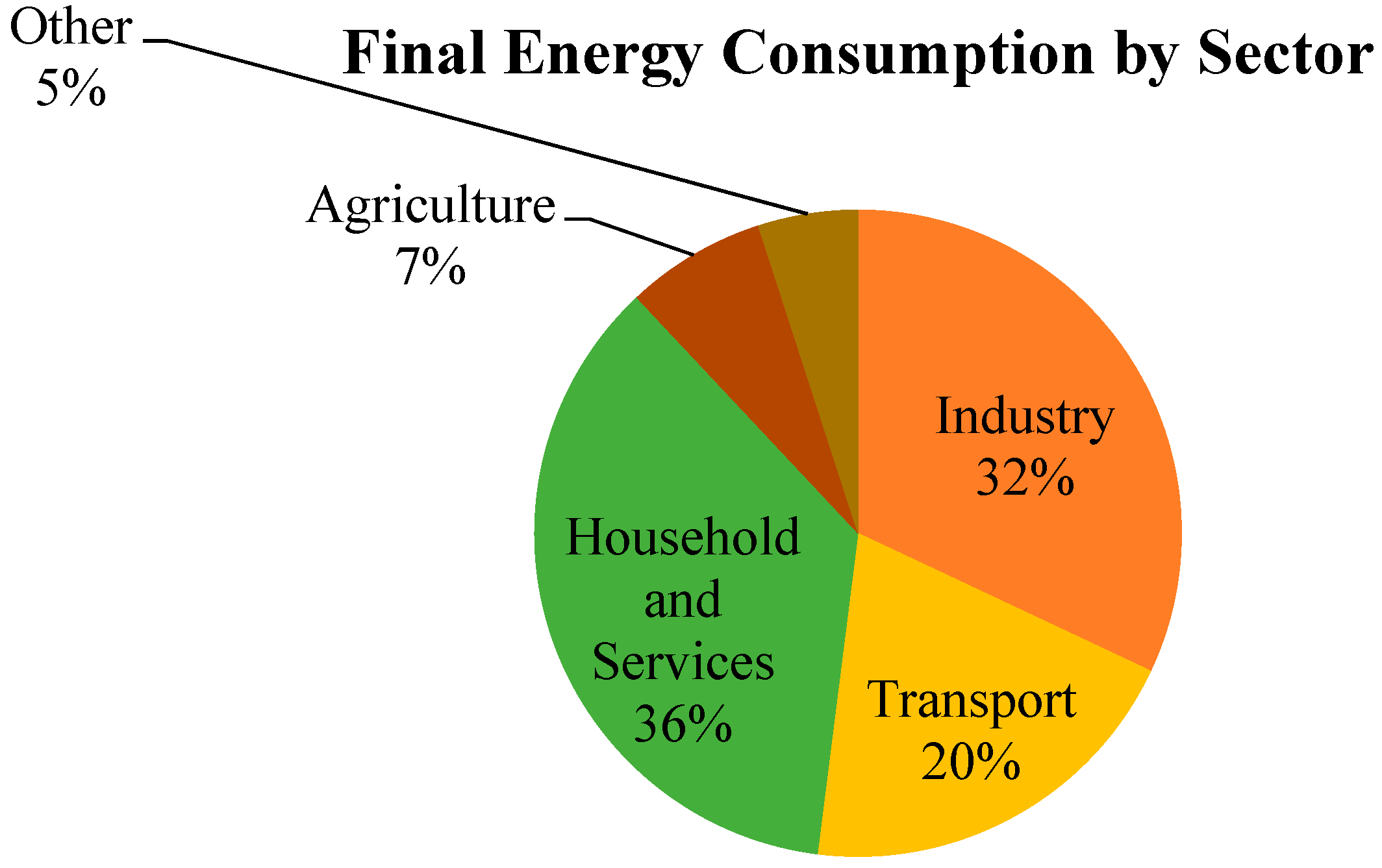
In Turkey, households and services are responsible for approximately 36 percent of total energy consumption in 2011 (Figure 3).
Buildings and household appliances are responsible for most household and service sector electricity consumption. As a result, several policies focus on these specifically. We use a highly stylized version of two of these policies and estimate the expected rise in efficiency. This energy efficiency increment is then applied in simulation to estimate difference in the associated rebound effect with and without energy theft by informal sectors and households.
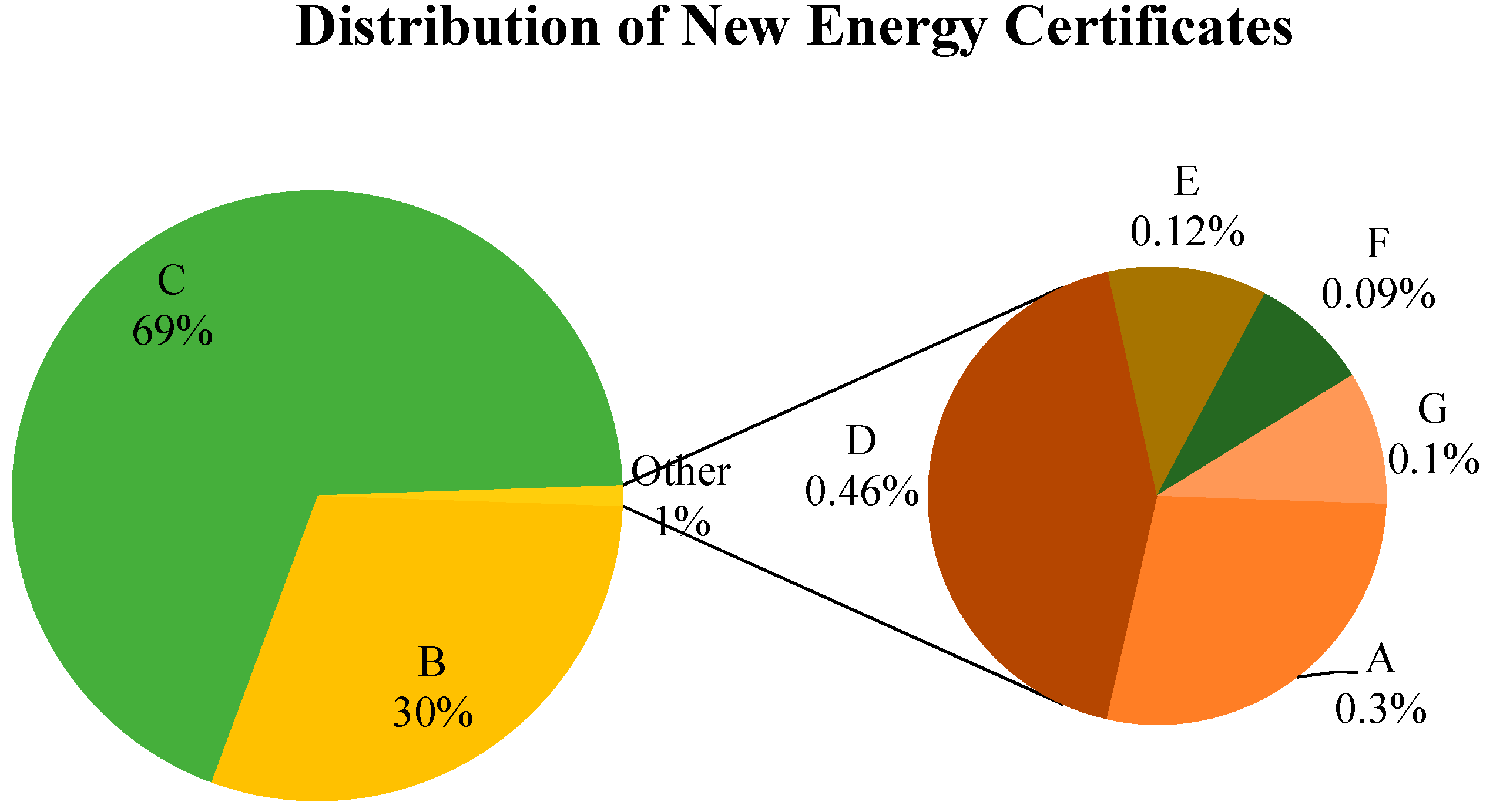
First the efficiency standard for buildings, undertaken according to the “Energy Performance Certificate” law. According to the law, energy performance will be calculated according to energy consumption levels and carbon dioxide emissions of each building. Buildings are grouped into 7 categories: A, B, C, D, E, F, or G, with A representing the most efficient buildings and G representing the least efficient.
In accordance with this law newly constructed buildings are required to meet at least a C level in order to qualify for a building permit. Moreover, all existing buildings must obtain a minimum C certificate by 2017 or face fines. While most new buildings meet only the minimum requirement, as shown in Figure 4 above, most existing buildings that had previously obtained certificates fell below the new minimum requirement. Therefore, as an efficiency increment we assume all existing buildings are improved to C level from G while all new buildings will be in the C category. In order to calculate an energy efficiency parameter, we used maximum the consumption level allowable for compliance with C and G certificates. Due to the policy, we see a 42 per cent increase in efficiency, as C buildings use approximately 58% of the energy of G buildings. This becomes a 42% energy efficiency increment φ for the service sector:
Equation x above shows the bundling of energy and capital to create the energy services used by production sectors I. The level of energy service provided in C buildings is assumed identical to that of G buildings, and the cost per unit of capital (for purposes of production) is assumed unchanged. For simplicity, this policy is modeled as a pure technological improvement rather than as an expensive retrofit [61].
The second policy that we introduce is mandatory energy efficiency labeling and minimum standards for household appliances. Energy labeling for household appliances is functionally similar to energy certification for buildings and groups them into seven categories according to their electricity consumption level.
We make the simplifying assumption that during the time period 2002–2014, the entirety of the energy efficiency change for that period has been a result of these policies, and this value is considered to be the energy efficiency increment or expected percentage decrease in energy use φ for production of the household energy service ESFH or ESNH. We compose a durable good bundle of energy and industrial goods, representing the “energy service” from usage of appliances by formal and informal households:
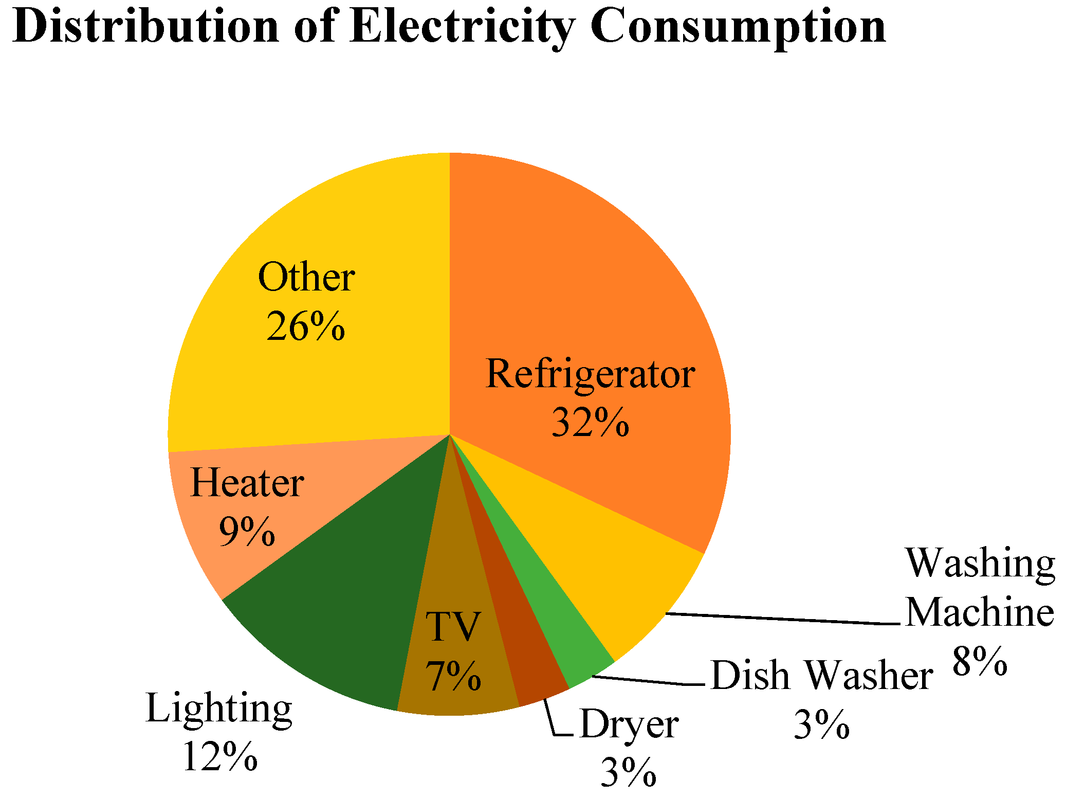
To calculate φ for households we use a weighted average of refrigerators, ovens, washing machines and dishwashers to represent appliances overall. Using datasets from the White Goods Manufacturers’ Association of Turkey (TURKBESD), for each appliance we evaluate which the most popular class in 2002 and 2014. The Chamber of Mechanical Engineers provide efficiency parameters for each class and each appliance enabling us to calculate the efficiency difference for each preferred appliance. After taking a weighted average, according to proportions shown in Figure 5, of their individual increments we estimate an overall 48 per cent energy efficiency increment for households. Again, for simplicity this is modeled as a pure technological improvement that neither increases the unit cost of appliances nor alters the quality of the energy service, an assumption that leads to a higher estimated rebound than would likely be the case for a costly policy [61]. For simplicity, it is assumed that households have the choice of only one appliance version, an energy inefficient one prior to the policy and an energy efficient one with identical cost after the policy.
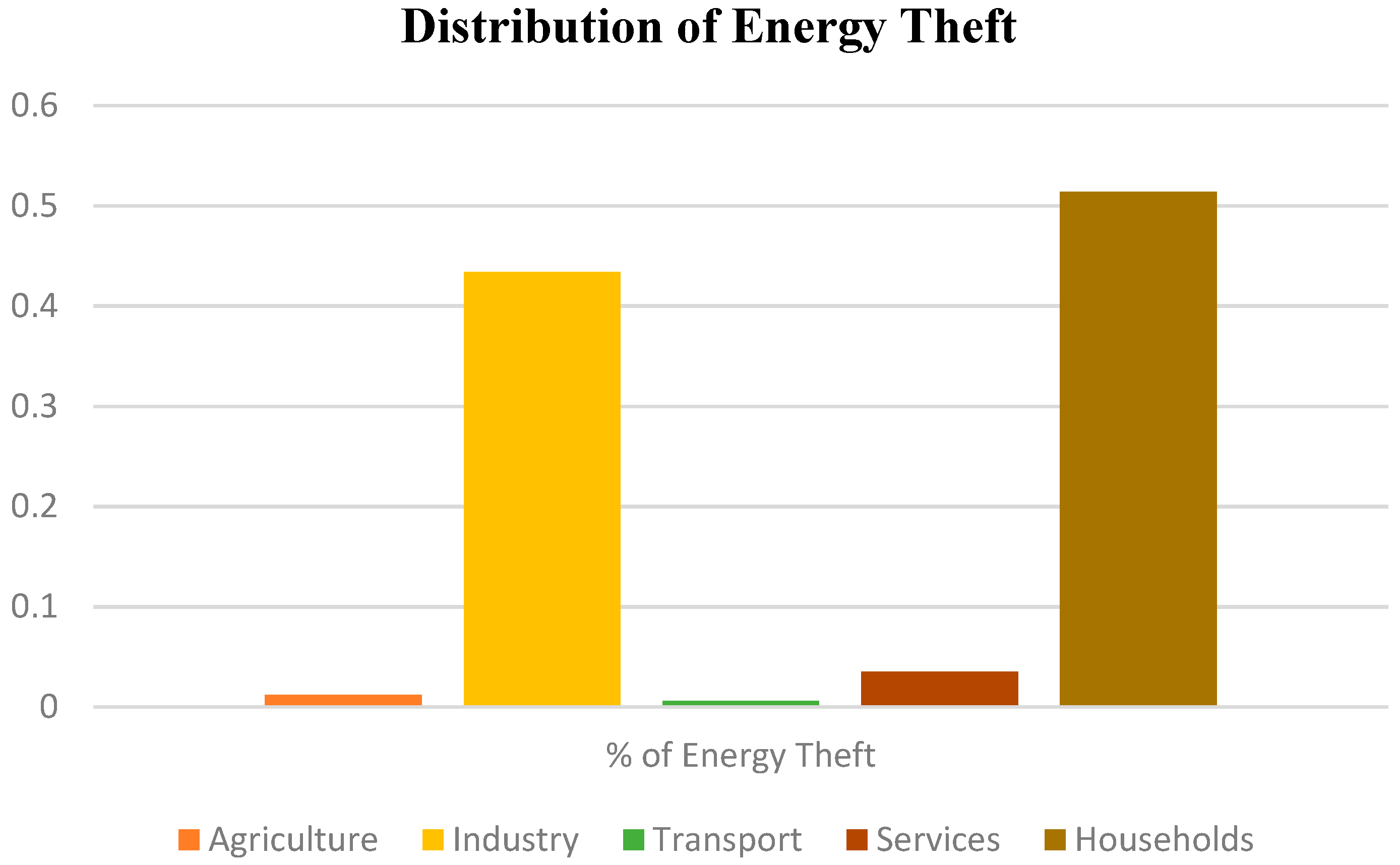
We assume a baseline level of energy theft of approximately 10.9% [33] of total energy consumed by households and sectors (the variable THEFT), equal to an estimate of the national average based on distributor-level data reported by EPDK for 2015. This gives a ratio of theft to sales equal to approximately 12.3%. The distribution of energy theft between informal sectors is assumed proportional to informal sector capital use; future changes in theft are assumed proportional to changes in capital use by these sectors. For the informal household group, future changes in theft are proportional to changes in consumption of (both formal and informal) industrial goods. In the absence of a price paid, there is no substitution between capital or industrial goods and energy by informal sectors or households, giving a Leontief bundle for production of the informal “energy service” while formal energy services follow a CES functional form. As a given representative agent consumes either an informal energy service or a formal energy service but not both, the model does not allow for substitution between the two. Initial proportions of overall energy theft can be seen below in Figure 6.
Formal sectors, as well as households and the government, must pay a uniform premium or markup τ, referred to as “Kayıp/Kaçak Bedeli” on users bills in Turkey, on energy purchases such that the energy sector is able to recover the costs of energy theft. This markup is the same for all user types, and is not dependent upon the prevalence of theft by that user type, approximately replicating the system currently in place in Turkey [62]. The markup functions as a tax, with the rate determined by the levels of (expected) energy theft and legal energy sales and revenues returned to the energy sector:
where τ represents the markup, THEFT the amount of energy stolen, QSHE the amount of legal energy sales (not to be confused with t, which denotes the value added tax). The initial value of the markup is approximately 12.3%, which is the rate necessary for the energy sector to recover the cost associated with the baseline amount of theft.
3. Results
We first present results for a series of simulations to set a baseline using the first model in which Turkey’s shadow economy and the phenomenon of energy theft are ignored. All sectors are treated as formal sectors, all energy consumed is paid for. Four cases are presented in Table 1 below, the first with no change in energy efficiency, the second with a 42% energy efficiency increment in building energy services used by the service sector, the third with a 48% energy efficiency increment in durable goods used by households and the fourth with energy efficiency improvements in both buildings and durable goods.
Due to the underlying structure of the model estimates of rebound in all four cases are small: less than 0.4%. This is primarily due to low assumed substitution elasticities between energy and non-energy goods, fixed factor supply and the limited export response [31]. The energy efficiency improvement affects households and the service sector, which exports relatively little of its output. The industrial sector, which dominates Turkish exports, sees no improvement in efficiency. Domestically, production in the service sector is far less energy intensive than the industrial sector. As a result, when the price of service sector output falls due to energy efficiency gains, this leads to substitution of services in place of industrial goods, which reduces energy consumption and leads to negative rebound for the energy efficiency improvement in buildings.
We next present our core results, estimates for the same four scenarios with Turkey’s shadow economy and the phenomenon of energy theft included. These four cases are presented in Table 2 below.
In the second case, the rebound associated with a 42% energy efficiency increment for buildings used by the service sector is substantially more negative at −7.8% when energy theft is included than when energy theft is ignored. There are two primary channels through which rebound is expected to be affected by the presence of electricity theft. The first is a direct effect: those who do not pay for energy will not see reductions in costs of production due to energy efficiency gains nor will they have an incentive to substitute more efficient energy-capital composites for other inputs as firms that pay for energy would. The second channel is indirect and less obvious: changes in the proportion of energy which is stolen affect the markup passed on to paying customers and thereby the price that they pay for energy. The Turkish formal service sector is estimated to represent a larger fraction of paid energy demand (7.5%) than the proportion of energy theft represented by the Turkish informal service sector (3.5%). As a result, the increase in building efficiency causes a greater reduction in energy sales than in energy theft. This causes an increase in the markup on energy, increasing the price paid by other formal sectors and suppressing energy demand by other formal sectors, which in this case causes a larger negative rebound.
The results for the third case, the 48% energy efficiency increment in household durable goods, show a very different effect of the inclusion of the shadow economy and energy theft. Unlike the service sectors, Turkish households represent a larger proportion of energy theft (51.4%) than of formal energy sales (28.5%). As a result, the energy efficiency gain in durable goods causes a larger drop in electricity theft than in formal electricity sales. The markup on electricity sales decreases, encouraging formal sector electricity consumption. Through the first channel, it remains true that there should be little or no direct rebound on household electricity theft from the energy efficiency gain, as the households will observe no reduction in the overall cost of the energy service. However, the indirect effect of the falling markup causes the rebound associated with efficiency gains for durable goods to rise from 0.4% without energy theft to almost 10.4% when the effects of energy theft are included. When both policies are included simultaneously, rebound remains substantially higher with energy theft (5.9%) than without (−0.4%).
The aforementioned results displayed in Table 1 and Table 2 assume an elasticity of substitution with the energy-service nest (ε) of 0.5, complementarity between energy and capital or energy and energy-using industrial goods. Table 3 and Table 4 display the results of sensitivity analysis for energy efficiency gains in buildings and durables with ε of 0.5, 1 and 2 within the energy nest. In the case of building efficiency gains without energy theft, a higher ε leads to a slightly positive rebound rather than the negative one in the baseline case. This is due to production sectors, rather than households, increasing energy use through substitution away from capital. In the model with energy theft, the rebound effect becomes progressively more negative as ε increases, reaching −19.7% when the elasticity is 2. As can be seen in Table 3, this is due to progressively larger decreases in paid energy consumption by formal sectors as ε increases rather than any change in energy theft.
As elasticity increases it becomes easier for these firms to substitute capital for energy, which has become more expensive as τ (the Kayıp Kaçak Bedeli or KKB surcharge) rises from 12.3% to 12.7% or 12.8%. Without energy theft, a higher ε leads to higher rebound for building efficiency improvements, whereas with energy theft a higher ε leads to a lower (more negative) rebound for building efficiency improvements due to the increase in τ.
For the energy efficiency improvement in durable goods, where energy theft is affected more strongly than paid energy consumption, the effect of increased ε is reversed. In the model without energy theft, increasing ε leads to small increases in rebound: from 0.4% to 1% to 2.1% for ε of 0.5, 1 and 2. In the model with energy theft, increasing ε also leads to greater rebound but with a dramatically larger effect than without energy theft: from 10.4% to 19.6% to 40.7% for ε of 0.5, 1 and 2 respectively. The dramatically larger rebound effect is due to the increase in energy consumption by formal production sectors, as they substitute into energy and away from capital as the price of energy falls due to the drop in τ.
4. Discussion
Previous studies have shown the importance of model structure, sectoral definitions and specific policy details in estimation of the size of the rebound associated with an energy efficiency increment. We add one further important factor which must be considered in estimating rebound, particularly in the case of middle-income or developing countries: the prevalence of energy theft and the impact of the specific policy or technological change on energy theft. Energy theft will always lead to smaller direct rebound effects, as benefits to energy users of efficiency gains will go unnoticed when energy is not paid for. However, mechanisms for the recovery of the costs associated with energy theft can have indirect effects on energy use and rebound that may be greater than these direct effects.
We have analyzed a specific mechanism for recovering the costs of energy theft, that which is employed in Turkey. In this mechanism, a uniform electricity surcharge (the KKB, or τ in the model) is imposed on all purchasers of electricity calibrated to recover the electrical utility’s expected cost of theft. As such all energy purchasing firms and households bear the burden, not only those considered likely to steal. Furthermore, there is a direct (though lagged in the Turkish policy case) connection between changes in theft and changes in the surcharge. We find that with such a mechanism, energy theft can lead to a small/negative or much larger indirect rebound effect depending upon whether the energy efficiency gain disproportionately affects energy theft or disproportionately affects legal energy sales.
In the Turkish case, policies to increase energy efficiency in the service sector disproportionately affect legal energy sales. As a result, when the costs associated with energy theft are recovered through a uniform surcharge as in Turkey the rebound associated with the policy is strongly negative. The reduction in energy use is substantially greater than the engineering estimate, super-conservation in the terminology of Saunders [30]. In other models, where differences in structure and specification lead to larger estimated rebound effects we would anticipate that the inclusion of energy theft with a uniform recovery surcharge would lead to substantially lower estimates of rebound. The policy that increases household energy efficiency disproportionately affects energy theft. As a result, when the costs associated with energy theft are recovered through a uniform recovery surcharge, the surcharge falls. This fall in the surcharge causes substantially higher estimates of rebound than without energy theft. These differences, relative to estimates obtained using a comparable model that does not include energy theft, are shown to be large enough that ignoring them may lead to a serious bias.
This study is the first to explore the impact of energy theft on estimation of the rebound effect associated with energy efficiency policy in developing countries. The understanding that energy efficiency policy may result in higher or lower recovery surcharges depending upon the relative impact of the policy on energy sales and energy theft will have a practical effect for policy makers. However, the model we have used for illustrative purposes is stylized and static with highly aggregated sectors, a simplified treatment of investment and international interactions and standard elasticity assumptions. More research should be done in those countries where energy theft is common to re-estimate rebound in those contexts using the detailed models that have been designed for those countries, but also incorporating energy theft along with specific country-specific cost recovery mechanisms. Furthermore, as our study focuses on the effect of current energy theft on rebound, we have little to say about the determinants of energy theft or about optimal energy policy where energy theft may occur. These issues will be important topics for future research.
Author Contributions
Conceptualization, T.S. and C.H.; methodology, C.H.; data curation, T.S.; Validation, T.S. and C.H.; formal analysis, C.H.; software, C.H.; writing—original draft, T.S. & C.H.; writing—review & editing, T.S. and C.H.
Funding
This research received no external funding.
Conflicts of Interest
The authors declare no conflict of interest.
Appendix A. Model with Informal Sectors and Energy Theft
Each model follows a standard neoclassical, perfectly competitive general equilibrium framework, with requisite closure rules, as in Arrow and Debreu [56]. Specific functional forms follow a constant elasticity of substitution specification as outlined in Rutherford [46] with a share calibrated from social accounting matrix data following Rutherford [45,47,49]. The specification for the inclusion of the energy efficiency increment follows Saunders [29].
Sets
Z (all industries and consumers) F all formal sectors and consumers, N all informal sectors and consumers with F as a subset of Z and N representing all elements of Z not in N. I represents all production sectors and is a subset of Z. E represents the energy sector, which is a member of F. FH and NH represent formal households and informal households, members of F and N respectively. . . . One set should represent non-energy firms: . , . .
Parameters
Any value refers to a baseline value of the variable or parameter X, which is endogenously determined within the general equilibrium model:
are calibrated scalar parameters to match the base year SAM data. represent energy efficiency increments for energy used in the respective energy service bundles. All φ parameters take a base value of unity. In the durable goods simulation, take on a value of 0.48.In the buildings simulation, take on a value of 0.42.
Production Functions:
Armington Aggregation:
Energy Service Bundling:
Durables Bundling:
Armington Version Intermediate Demands:
Intermediate Demands:
Final Demands:
Cost Functions (and Zero-Profit Conditions):
Market Clearance:
Income:
Electricity Theft:
Appendix B. Model without Informal Sectors or Energy Theft
Sets
Z (all industries and consumers) F all formal sectors and consumers with F as a subset of Z. I represents all production sectors and is a subset of Z. E represents the energy sector, which is a member of F. FH represents formal households. . . Industry Categories: . . .
Parameters
are calibrated scalar parameters to match the base year SAM data represent energy efficiency increments for energy used in the respective energy service bundles. All φ parameters take a base value of unity. In the durable goods simulation, takes on a value of 0.48. In the buildings simulation, takes on a value of 0.42.
Production Functions:
Armington Aggregation:
Energy Service Bundling:
Durables Bundling:
Armington Version Intermediate Demands:
Intermediate Demands:
Final Demands:
Cost Functions (and Zero-Profit Conditions):
Market Clearance:
Income:
References
- Sorrell, S. Jevons’ Paradox revisited: The evidence for backfire from improved energy efficiency. Energy Policy 2009, 37, 1456–1469. [Google Scholar] [CrossRef]
- Greening, L.A.; Greene, D.L.; Difiglio, C. Energy efficiency and consumption—The rebound effect—A survey. Energy Policy 2000, 28, 389–401. [Google Scholar] [CrossRef]
- Barker, T.; Dagoumas, A.; Rubin, J. The Macroeconomic Rebound Effect and the World Economy. Energy Effic. 2009, 2, 411–427. [Google Scholar] [CrossRef]
- IEA. (2009) Energy Policies of IEA Countries: Turkey 2009 Review. Available online: https://webstore.iea.org/energy-policies-of-iea-countries-turkey-2009-review (accessed on 15 October 2018).
- Smith, T.B. Electricity theft: A comparative analysis. Energy Policy 2004, 32, 2067–2076. [Google Scholar] [CrossRef]
- Lovins, A.B. Energy saving resulting from the adoption of more efficient appliances: Another view. Energy J. 1988, 9, 155–162. [Google Scholar] [CrossRef]
- Wirl, F. The Economics of Conservation Programs; Springer Science & Business Media: New York, NY, USA; p. 1997. ISBN 9781461563013.
- Alcott, B. Jevons’ paradox. Ecol. Econ. 2005, 54, 9–21. [Google Scholar] [CrossRef]
- Khazzoom, J.D. Economic implications of mandated efficiency in standards for household appliances. Energy J. 1980, 1, 21–40. [Google Scholar]
- Khazzoom, J.D. Energy saving resulting from the adoption of more efficient appliances. Energy J. 1987, 8, 85–89. [Google Scholar]
- Khazzoom, J.D. Energy savings from more efficient appliances: A rejoinder. Energy J. 1989, 10, 157–166. [Google Scholar]
- Brookes, L.G. More on the output elasticity of energy consumption. J. Ind. Econ. 1972, 21, 83–92. [Google Scholar] [CrossRef]
- Brookes, L. The greenhouse effect: The fallacies in the energy efficiency solution. Energy Policy 1990, 18, 199–201. [Google Scholar] [CrossRef]
- Schipper, L.; Grubb, M. On the rebound? Feedback between energy intensities and energy uses in IEA countries. Energy Policy 2000, 28, 367–388. [Google Scholar] [CrossRef]
- Saunders, H.D. The Khazzoom-Brookes Postulate and Neoclassical Growth. Energy J. 1992, 13, 131–148. [Google Scholar] [CrossRef]
- Dimitropoulos, J. Energy Productivity Improvements and the Rebound Effect: An Overview of the State of Knowledge. Energy Policy 2007, 35, 6354–6363. [Google Scholar] [CrossRef]
- Semboja, H.H. The effects of an increase in energy efficiency on the Kenya economy. Energy Policy 1994, 22, 217–225. [Google Scholar] [CrossRef]
- Glomsrød, S.; Taoyuan, W. Coal cleaning: A viable strategy for reduced carbon emissions and improved environment in China? Energy Policy 2005, 33, 525–542. [Google Scholar] [CrossRef]
- Lu, Y.; Liu, Y.; Zhou, M. Rebound Effect of Improved Energy Efficiency for Different Energy Types: A General Equilibrium Analysis for China. Energy Econ. 2017, 62, 248–256. [Google Scholar] [CrossRef]
- Dufournaud, C.M.; Quinn, J.T.; Harrington, J.J. An applied general equilibrium (AGE) analysis of a policy designed to reduce the household consumption of wood in the Sudan. Resour. Energy Econ. 1994, 16, 67–90. [Google Scholar] [CrossRef]
- Vikström, P. Energy efficiency and energy demand: A historical CGE investigation on the rebound effect in the Swedish economy 1957. Umeå Pap. Econ. Hist. 2008, 35, 1–27. [Google Scholar]
- Broberg, T.; Berg, C.; Samakovlis, E. The economy-wide rebound effect from improved energy efficiency in Swedish industries—A general equilibrium analysis. Energy Policy 2015, 83, 26–37. [Google Scholar] [CrossRef]
- Washida, T. Economy-wide model of rebound effect for environmental efficiency. In Proceedings of the International Workshop on Sustainable Consumption, Leeds, UK, 5–6 March 2004. [Google Scholar]
- Allan, G.; Hanley, N.; McGregor, P.G.; Swales, J.K.; Turner, K. The Macroeconomic Rebound Effect and the UK Economy. Final Report to DEFRA 2006. Available online: https://strathprints.strath.ac.uk/7254/ (accessed on 15 October 2018).
- Hanley, N.; McGregor, P.G.; Swales, J.K.; Turner, K. The impact of a stimulus to energy efficiency on the economy and the environment: A regional computable general equilibrium analysis. Renew. Energy 2006, 31, 161–171. [Google Scholar] [CrossRef]
- Lecca, P.; Mcgregor, P.G.; Swales, J.K.; Turner, K. The Added Value from a General Equilibrium Analysis of Increased Efficiency in Household Energy Use. Ecol. Econ. 2014, 100, 51–62. [Google Scholar] [CrossRef] [Green Version]
- Grepperud, S.; Rasmussen, I. A general equilibrium assessment of rebound effects. Energy Econ. 2004, 26, 261–282. [Google Scholar] [CrossRef]
- Wei, T.; Liu, Y. Estimation of global rebound effect caused by energy efficiency improvement. Energy Econ. 2017, 66, 27–34. [Google Scholar] [CrossRef]
- Koesler, S.; Swales, J.K.; Turner, K. International spillover and rebound effects from increased energy efficiency in Germany. Energy Econ. 2016, 54, 444–452. [Google Scholar] [CrossRef] [Green Version]
- Saunders, H.D. Fuel conserving (and using) production functions. Energy Econ. 2008, 30, 2184–2235. [Google Scholar] [CrossRef]
- Saunders, H.D. Recent evidence for large rebound: Elucidating the drivers and their implications for climate change models. Energy 2015, 36, 23–48. [Google Scholar] [CrossRef]
- Freire-Gonzalez, J. A new way to estimate the direct and indirect rebound effect and other rebound indicators. Energy 2017, 128, 394–402. [Google Scholar] [CrossRef]
- Enerji Piyasası Düzenleme Kurumu (EPDK). Elektrik Piyasası 2015 Yılı Piyasa Gelişim Raporu; EPDK: Ankara, Turkey, 2016. [Google Scholar]
- TEDAŞ. Yili Faaliyet Raporu, August 2012. Available online: http://www.tedas.gov.tr/sx.web.docs/tedas/docs/faaliyetrapor/2011_yili_faaliyet_raporu.pdf (accessed on 16 October 2018).
- Yurtseven, Ç. The causes of electricity theft: An econometric analysis of the case of Turkey. Util. Policy 2015, 37, 70–78. [Google Scholar] [CrossRef]
- Tasdoven, H.; Fiedler, B.A.; Garayev, V. Improving electricity efficiency in Turkey by addressing illegal electricity consumption: A governance approach. Energy Policy 2012, 43, 226–234. [Google Scholar] [CrossRef]
- Ulusoy, A.; Oguz, F. The privatization of electricity distribution in Turkey: A legal and economic analysis. Energy Policy 2007, 35, 5021–5034. [Google Scholar] [CrossRef]
- Gümüşdere, E. Theft and Losses in Turkish Electricity Sector. Ph.D. Dissertation, Sabanci University, Istanbul, Turkey, 2004. Available online: http://research.sabanciuniv.edu/8235/ (accessed on 15 October 2018).
- Schneider, F.; Buehn, A.; Montenegro, C.E. Shadow Economies all over the World: New Estimates for 162 Countries from 1999 to 2007; World Bank Policy Research Working Paper Series; The World Bank Group: Washington, DC, USA, 2010. [Google Scholar] [CrossRef]
- Gibson, B.; Kelley, B. A classical theory of the informal sector. Manch. Sch. 1994, 62, 81–96. [Google Scholar] [CrossRef]
- Kelley, B. The informal sector and the macroeconomy: A computable general equilibrium approach for Peru. World Dev. 1994, 22, 1393–1411. [Google Scholar] [CrossRef]
- Armington, P.S. A theory of demand for products distinguished by place of production. Staff. Pap. (Int. Monet. Fund) 1969, 16, 159–178. [Google Scholar] [CrossRef]
- Gibson, B. The transition to a globalized economy: Poverty, human capital and the informal sector in a structuralist CGE model. J. Dev. Econ. 2005, 78, 60–94. [Google Scholar] [CrossRef]
- Schaefer, K.K. Capacity Utilization, Income Distribution, and the Urban Informal Sector: An Open-Economy Model. PERI Working Papers 2002. Available online: https://scholarworks.umass.edu/peri_workingpapers/19/ (accessed on 15 October 2018).
- Rutherford, T.F. CES Preferences and Technology: A Practical Introduction. Economic Equilibrium Modeling with GAMS: An Introduction to GAMS/MCP and GAMS/MPSGE (GAMS/MPSGE Solver Manual). 1998, pp. 89–115. Available online: https://www.gams.com/latest/docs/mpsge.pdf (accessed on 15 October 2018).
- Rutherford, T.F. Applied general equilibrium modeling with MPSGE as a GAMS subsystem: An overview of the modeling framework and syntax. Comput. Econ. 1999, 14, 1–46. [Google Scholar] [CrossRef]
- Rutherford, T.F. Lecture Notes on Constant Elasticity Functions, University of Colorado. 2002. Available online: http://citeseerx.ist.psu.edu/viewdoc/download?doi=10.1.1.364.2392&rep=rep1&type=pdf (accessed on 15 October 2018).
- Rutherford, T.F. Calibrated CES Utility Functions: A Worked Example. Mimeo, ETH Zürich, 2008. Available online: https://pdfs.semanticscholar.org/01f6/10fed07cdf71b65b5c0a23354bb13d553a3e.pdf (accessed on 15 October 2018).
- Leontief, W.W. Quantitative input and output relations in the economic systems of the United States. Rev. Econ. Stat. 1936, 105–125. [Google Scholar] [CrossRef]
- Timmer, M.P.; Dietzenbacher, E.; Los, B.; Stehrer, R.; de Vries, G.J. An Illustrated User Guide to the World Input–Output Database: The Case of Global Automotive Production. Rev. Int. Econ. 2015, 23, 575–605. [Google Scholar] [CrossRef]
- University of Cambridge. Department of Applied Economics, Alan Brown and Richard Stone. A Programme for Growth: A Social Accounting Matrix for 1960; Chapman and Hall: London, UK, 1962. [Google Scholar]
- Schneider, F. The Shadow Economy and Work in the Shadow: What Do We (Not) Know?” IZA Discussion Paper No. 6423. 2012. Available online: https://ssrn.com/abstract=2031951 (accessed on 15 October 2018).
- Schneider, F.; Kearney, A.T. The Shadow Economy in Europe, 2013; Johannes Kepler Universitat: Linz, Austria, 2013. [Google Scholar]
- Del Bo, C.; Fiorio, C.; Florio, M. Shadow Wages for the EU Regions. Fisc. Stud. 2011, 32, 109–143. [Google Scholar] [CrossRef]
- Cantekin, K.; Elgin, C. Extent and Growth Effects of Informality in Turkey: Evidence form a Firm-Level Survey. Singap. Econ. Rev. 2015, 62, 1017–1037. [Google Scholar] [CrossRef]
- Arrow, K.J.; Debreu, G. Existence of an equilibrium for a competitive economy. Econ. J. Econ. Soc. 1954, 265–290. [Google Scholar] [CrossRef]
- Berndt, E.R.; Wood, D.O. Technology, prices, and the derived demand for energy. Rev. Econ. Stat. 1975, 57, 259–268. [Google Scholar] [CrossRef]
- Griffin, J.M.; Gregory, P.R. An intercountry translog model of energy substitution responses. Am. Econ. Rev. 1976, 66, 845–857. [Google Scholar]
- Magnus, J.R. Substitution between energy and non-energy inputs in the Netherlands 1950–1976. Int. Econ. Rev. 1979, 20, 465–484. [Google Scholar] [CrossRef]
- Kemfert, C.; Welsch, H. Energy-Capital-Labor Substitution and the Economic Effects of CO2 Abatement: Evidence for Germany. J. Policy Model. 2000, 22, 641–660. [Google Scholar] [CrossRef]
- Gillingham, K.; Rapson, D.; Wagner, G. The rebound effect and energy efficiency policy. Rev. Environ. Econ. Policy 2016, 10, 68–88. [Google Scholar] [CrossRef]
- Çolak, N.; Demir, Z. Elektrik fiyatını belirleyen bileşenler. In Proceedings of the 1st International Workshop on Construction and Electricity Applications on Vocational Education, Anadolu University, Ankara, Turkey, 30 November 2015; Available online: http://iwcea2015.anadolu.edu.tr/sites/iwcea2015.anadolu.edu.tr/files/files/iwcea2015_proceedings_book.pdf (accessed on 15 October 2018).
Figure 1.
Model structure of utility generation through household consumption.

Figure 2.
Structure of domestic production of goods and services.

Figure 3.
Sectoral Breakdown of Final Energy Consumption (2008).

Source: MENR
Figure 4.
Distribution of New Building Energy Certificates by 2015 (after policy).

Source: BEP
Figure 5.
Distribution of Energy Consumption by Appliance.

Source: TURKBESD
Figure 6.
Distribution of Energy Theft by Sector.


Table 1.
Turkey Model Estimation, no Informal Sector or Energy Theft.
| Variable | Buildings | Durables | Buildings & Durables |
|---|---|---|---|
| Expected Energy Use Reduction | 4.15% | 10.20% | 14.41% |
| Actual Energy Use Reduction | 4.09% | 10.16% | 14.35% |
| Rebound | −1.5% | 0.4% | −0.4% |
| Change in Welfare | 0.3% | 0.6% | 0.9% |
Table 2.
Turkey Model Estimation with Informal Sector and Energy Theft.
| Variable | Buildings | Durables | Buildings & Durables |
|---|---|---|---|
| Expected Energy Sales Reduction | 4.07% | 10.65% | 14.66% |
| Expected Energy Theft Reduction | 1.47% | 24.67% | 26.14% |
| Actual Energy Sales Reduction | 4.35% | 9.3% | 13.7% |
| Actual Energy Theft Reduction | 1.4% | 24.3% | 25.8% |
| Rebound | −7.8% | 10.4% | 5.9% |
| Energy Price Markup Due to Theft (base 10.5%) | 12.7% | 10.3% | 10.6% |
| Change in Formal Household Welfare | 0.1% | 0.8% | 1.0% |
| Change in Shadow Household Welfare | 0.1% | 0.3% | 0.6% |
Table 3.
Building Efficiency, Sensitivity of Results to Elasticity of Substitition within Energy Nest.
Table 3.
Building Efficiency, Sensitivity of Results to Elasticity of Substitition within Energy Nest.
| Variable | Sector | Without Energy Theft | With Energy Theft | ||||
|---|---|---|---|---|---|---|---|
| ε = 0.5 | ε = 1 | ε = 2 | ε = 0.5 | ε = 1 | ε = 2 | ||
| Energy use | Agriculture | −0.05% | 0.04% | 0.22% | −0.29% | −0.43% | −0.79% |
| (theft) | −0.1% | −0.1% | −0.1% | ||||
| Industry | −0.19% | −0.11% | 0.04% | −0.46% | −0.58% | −0.88% | |
| (theft) | −0.0% | −0.0% | −0.0% | ||||
| Service | −41.72% | −41.66% | −41.56% | −41,83% | −41,91% | −42,12% | |
| (theft) | −42.0% | −42.0% | −42.0% | ||||
| Transport | −0.01% | 0.08% | 0,26% | −0.23% | −0.38% | −0.73% | |
| (theft) | −0.0% | −0.0% | −0.1% | ||||
| Energy | −4.18% | −4.08% | −3.88% | −4.26% | −4.44% | −4.90% | |
| Households | 0.15% | 0.14% | 0.12% | −0.10% | −0.32% | −0.82% | |
| (theft) | +0.2% | +0.2% | +0.2% | ||||
| Government | 0.42% | 0.42% | 0.42% | −0.12% | −0.15% | −0.22% | |
| Total Change | −4.15% | −4.08% | −3.96% | −4.02% | −4.15% | −4.46% | |
| Exected Change | −4.09% | −4.09% | −4.09% | −3.73% | −3.73% | −3.73% | |
| Other | Rebound | −1.5% | +0.1% | +3.1% | −7.8% | −11.3% | −19.7% |
| Theft Markup (τ) | - | - | - | 12.7% | 12.7% | 12.8% | |
| Welfare Change | +0.3% | +0.3% | +0.2% | +0.2% | +0.2% | +0.2% | |
| Government Revenue Change | +0.6% | +0.6% | +0.6% | +0.5% | +0.5% | +0.5% | |
Table 4.
Durables Efficiency, Sensitivity of Results to Elasticity of Substitution within Energy Nest.
Table 4.
Durables Efficiency, Sensitivity of Results to Elasticity of Substitution within Energy Nest.
| Variable | Sector | Without Energy Theft | With Energy Theft | ||||
|---|---|---|---|---|---|---|---|
| ε = 0.5 | ε = 1 | ε = 2 | ε = 0.5 | ε = 1 | ε = 2 | ||
| Energy use | Agriculture | +0.24% | +0.33% | +0.50% | +1.32% | +2.87% | +6.43% |
| (theft) | +0.3% | +0.3% | +0.4% | ||||
| Industry | −0.18% | −0.11% | +0.04% | +1.09% | +2.41% | +5.40% | |
| (theft) | +0.4% | +0.4% | +0.4% | ||||
| Service | +0.63% | +0.72% | +0.89% | +2.01% | +3.55% | +7.10% | |
| (theft) | +0.3% | −0.3% | +0.4% | ||||
| Transport | +0.27% | +0.36% | +0.53% | +1.43% | +2.97% | +6.51% | |
| (theft) | +0.2% | +0.2% | +0.3% | ||||
| Energy | −10.18% | −10.08% | −9.88% | −9.92% | −8.17% | −4.10% | |
| Households | −47.63% | −47.62% | −47.61% | −46.88% | −46.21% | −44.57% | |
| (theft) | −47.44% | −47.79% | −47.84% | ||||
| Government | +1.91% | +1.91% | +1.92% | +5.29% | +5.52% | +6.06% | |
| Total Change | −10.16% | −10.09% | −9.96% | −10.92% | −9.80% | −7.23% | |
| Exected Change | −10.2% | −10.2% | −10.2% | −12.18% | −12.18% | −12.18% | |
| Other | Rebound | +0.4% | +1% | +2.3% | +10.4% | +19.6% | +40.7% |
| Theft Markup (τ) | - | - | - | 10.3%% | 10.1%% | 9.8% | |
| Welfare Change | +0.6% | +0.6% | +0.6% | +0.8% | +0.8% | +0.7% | |
| Government Revenue Change | +2.1% | +2.1% | +2.1% | +3.1% | +3.1% | +3.1% | |
© 2018 by the authors. Licensee MDPI, Basel, Switzerland. This article is an open access article distributed under the terms and conditions of the Creative Commons Attribution (CC BY) license (http://creativecommons.org/licenses/by/4.0/).
Share and Cite
MDPI and ACS Style
Somuncu, T.; Hannum, C. The Rebound Effect of Energy Efficiency Policy in the Presence of Energy Theft. Energies 2018, 11, 3379. https://doi.org/10.3390/en11123379
AMA Style
Somuncu T, Hannum C. The Rebound Effect of Energy Efficiency Policy in the Presence of Energy Theft. Energies. 2018; 11(12):3379. https://doi.org/10.3390/en11123379
Chicago/Turabian StyleSomuncu, Tugba, and Christopher Hannum. 2018. "The Rebound Effect of Energy Efficiency Policy in the Presence of Energy Theft" Energies 11, no. 12: 3379. https://doi.org/10.3390/en11123379
Note that from the first issue of 2016, this journal uses article numbers instead of page numbers. See further details here.