Electric Load Data Compression and Classification Based on Deep Stacked Auto-Encoders

Abstract

With the development of advanced metering infrastructure (AMI), electrical data are collected frequently by smart meters. Consequently, the load data volume and length increase dramatically, which aggravates the data storage and transmission burdens in smart grids. On the other hand, for event detection or market-based demand response applications, load service entities (LSEs) want smart meter readings to be classified in specific and meaningful types. Considering these challenges, a stacked auto-encoder (SAE)-based load data mining approach is proposed. First, an innovative framework for smart meter data flow is established. On the user side, the SAEs are utilized to compress load data in a distributed way. Then, centralized classification is adopted at remote data center by softmax classifier. Through the layer-wise feature extracting of SAE, the sparse and lengthy raw data are expressed in compact forms and then classified based on features. A global fine-tuning strategy based on a well-defined labeled subset is embedded to improve the extracted features and the classification accuracy. Case studies in China and Ireland demonstrate that the proposed method is more capable to achieve the minimum of error and satisfactory compression ratios (CR) than benchmark compressors. It also significantly improves the classification accuracy on both appliance and house level datasets.

1. Introduction

With the wide integration of distributed generations, a two-way power flow occurs frequently in modern power systems [1]. A similar bi-directional flow also appears in the information transmission of power systems due to advanced metering infrastructure (AMI) and some control systems [2,3]. Smart meters, the basic terminal equipment of AMI, have gained increasing popularity worldwide. By the end of 2016, smart meters installed in the UK and the US reached 2.9 million [4] and 70 million [5], respectively. There will be an unusual volume of collected readings from smart meters that should be transmitted simultaneously through limited- bandwidth environment. With the rapidly increasing volume of smart meter data, to transmit and store load data in a large service area is a realistic challenge for load service entities (LSEs). For instance, the volume of load profile data at a granularity of 1s and double-precision floating point for the 40 million households in Germany amounts to 25 TB per day [6]. It is practically unnecessary to keep the complete raw load data, considering an obvious redundancy. This can be explained in two aspects: (i) Load data is of sparsity itself, i.e., for the majority of users, high electricity consumption occurs only at a small fraction of time, while the rest of the data is or near zero [7]; (ii) Generality exists in users’ electricity consumption behaviors, in other words, load profiles share some common patterns, especially for some manufacturing and commercial customers with fixed job shifts [8,9]. Considering the redundancy, load data can be expressed in compact forms. Consequently, the load data compression has become a valuable work for LSEs.

According to the International Council on Large Electric Systems (CIGRE) [10], advanced applications including automatic metering, load forecasting and energy feedback can be achieved by smart meters. Generally, user segmentation is the fundamental step for further application of smart meter readings. Classification provides a straightforward recognition about loads, which should assign the loads in the same class sharing similar patterns, while loads in different classes illustrate significant differences. Based on classification, differentiated mechanisms are designed. Specifically, different Real-time Pricing (RTP), Time-of-use (TOU), or Critical Peak Pricing (CPP) levels are carried out to promote demand response (DR) for different user classes [11]. Future power demands are estimated using different methods or models for classes with respective growing trends [12]. Based on the above, load data compression and classification is considered as the main issue of this paper.

Data compression in smart grid has received considerable attention in recent years [13]. Generally, the utilized methods can be classified into lossless and lossy categories [12], depending on whether or not all original data can be recovered.

For lossless compression, the algorithms developed for audio and image signals, such as LZP2, FLAC, TTAEnc, ZIP, JPEG-LS, and JPEG2000-lossless were introduced for power quality event data in [14]. A Golomb–Rice encoding of Phasor Measurement Unit (PMU) data was exploited in [15]. Abuadbba et al. [6] proposed a Gaussian approximation lossless compression for smart meter readings. Unterweger et al. [16] invented a load data resumable compression utilizing differential coding and entropy coding. Ringwelski et al. [17] compared the existing standard approaches and provides a hitchhiker’s guide for lossless compression.

Lossy compression provides higher compression ratio (CR) at the expense of information loss. Reference [18] exploited the effects of using the symbolic aggregate approximation (SAX) for lossy load data compression. A feature-based method in [19] identified load features from the uncompressed data. A Gaussian mixture model was presented in [20], which exploited the sparsity of data to devise an adaptive lossy compression. Reference [11] and [21] introduced the Singular Value Decomposition (SVD) to reconstruct smart meter readings, the loss of this method is determined by the number of the reserved Singular Values ordered from the highest to the lowest. Reference [22] proposed an alternative to decompose smart meter data in the spectral domain. Other reported lossy methods include the Mixed Parametric and Transform Coding [23], Principal Component Analysis (PCA) [24], the Wavelet Transform [25,26], the Discrete Fourier Transform (DFT) [27], etc.

Due to the limited bandwidth and storage space, lossy compression is considered to be more promising in smart grid. Most of the above lossy methods are linear, whose information loss grows rapidly with the increasing CR. Consequently, the extendibility is limited [18,19,20,21,22,23,24,25,26,27]. On the other hand, the reported coding and decoding algorithms cannot provide satisfactory robustness on different datasets, which may hamper the software development and realistic practice.

Research has been conducted for load data classification or customer segmentation. In general, loads can be clustered through unsupervised and supervised ways [11]. Unsupervised methods such as k-means, hieratical clustering [28], and Self Organizing Map (SOM) [29] classify loads based on the Euclidean distance, density, or other data features. While, supervised methods identify unknown loads by learning the existing load classification statistical rules. Typical supervised methods include the Support Vector Machines (SVM) [7], the Decision Tree (DT), the Logistic Regression (LR) and the Naive Bayes (NB) classifier [28]. With a better understanding of data value, supervised classification has become the mainstream in recent researches and traditional unsupervised classification is often used as benchmark to assess the quality of new reported supervised methods.

With the development of smart grid and electricity market, new challenges and requirements arise for load data mining.

(1)

High quality smart meters collect data frequently and the historical measurements accumulate constantly, the data volume increases dramatically [5]. Besides, for some special issues, wider profiles are utilized [9,30], e.g., the weekly, monthly, or even annual load profiles. These developments require the load data to be compressed in higher ratios.

(2)

With the development of DR, user segmentation has received unprecedented attention recently [11]. Users should be classified into more specific and meaningful types. In non-intrusive load identification, the readings are investigated to match the household appliances [24,31], e.g., refrigerator and air conditioner.

In order to address the above challenges, this paper aims to achieve higher CRs for load data compression and better accuracies for load classification. Specifically, the concept and model of deep learning in Artificial Intelligence (AI) is introduced. Load data are compressed in a layer-wise way by Deep Stacked Auto-Encoders (SAEs) and the probability characteristics of load classification are obtained with a softmax regression method. The main contributions of the proposed method can be presented as follows:

(A)

An innovative framework for smart grid data flow. Specifically, encoders are installed or integrated at the user side to compress the collected smart meter readings to smaller volumes. The compressed data are transmitted to the remote data center for storage. The corresponding decoders are preconfigured in the data center, which can recover the compressed data if needed. In this way, both the transmission bandwidth and the storage space are reduced without affecting the further application and value-added services.

(B)

An efficient and adaptive Artificial Neural Network (ANN)-based compressor. Stacked Auto-Encodes (SAEs) are introduced to compress smart meter data. The SAE-based nonlinear compressor achieves satisfactory minimum of information loss when load data are compressed to extremely small sizes. By adjusting the number of neurons, the output data of SAE can be compressed to any configurable size and the model can adapt to various input dimensions. Compared with the state-of-the-art linear methods (PCA, DWT, and SVD), the proposed SAE model achieves higher CRs with a satisfactory minimum of information loss meanwhile.

(C)

A labeled data driven improvement for classification. Specifically, massive unlabeled data are classified by softmax classifier in data center based on features extracted by distributed SAEs. A following-up training is implemented to fine-tune all the weights based on well-defined labeled subset after pre-training, which greatly modifies the high order features and improves the classification accuracy. Numerical results demonstrate the proposed ANN-based method has a significantly better fit for both building level user segmentation and appliance level abnormal event detection.

The organization of the rest of this paper is as follows. Section 2 gives the framework of the proposed method. Section 3 provides some preprocessing techniques to make the raw data fit for ANN. Section 4 introduces the basic Auto-Encoder (AE) to encode and decode smart meter data. Section 5 elaborates the softmax regression for load profile classification. Based on AE and softmax classifier, Section 6 provides a deep ANN stacked by AEs for load data mining. Real smart meter datasets in China and Ireland are utilized for case studies in Section 7 to demonstrate the feasibility of the proposed approach. Finally, the conclusions are presented in Section 8.

2. Framework of the Proposed ANN-Based Load Data Compression and Classification Model

In this section, framework of the ANN-based load data compression and classification model is elaborated. With a distributed hierarchical structure, the proposed model consists of three parts, an encoding network, a decoding network, and a classification network.

The deployment of the three parts is shown in Figure 1. Encoding networks are installed or integrated at the user side to compress the collected smart meter readings to smaller volumes. The compressed data are transmitted to the remote data center for storage. In this way, both the transmission bandwidth and the storage space are greatly reduced. The corresponding decoding network is preconfigured in the data center and it can reconstruct the compressed data to its original length if needed. The compressed or reconstructed data can also be input into the classification network for identifying the labels or categories of the corresponding users or profiles. Some further applications are designed based on the estimated labels, etc., power billing, fault detection, or demand response. Messages about these applications are sent to the corresponding users, after that. In this paper, for a higher accuracy, loads are classified based on the compressed data. The proposed framework is easy to achieve in reality as the needed hardware are programmable chips such as the Field Programmable Gate Array (FPGA) [32], the Very Large Scale Integration (VLSI) [33], and Digital Signal Processing(DSP) [34].

Specifically, AE is utilized as the basic functional unit to encode and decode massive load data. Softmax regression is the recommended method for load classification. Inspired by the revolutionary progresses in deep learning, multiple AEs are stacked to constitute the compressor in order to provide better compression capability [35,36]. A fine-tuning strategy based on labeled load data is utilized to train the stacked AEs for a layer-wise compression of the redundant smart meter data [37].

3. Preprocessing of Load Data

In this section, some necessary preprocessing techniques utilized to make the raw data fit for ANN input are illustrated.

Suppose a dataset with K n-dimension load curves is obtained. Each curve can be denoted as X_i = (X_1i, X_2i,…, X_ni)^T. First, a min-max data normalization is implemented [38].

$$x_{i,j}=\frac{X_{i,j}-{\min }_{i=1}^n\left(X_{i,j}\right)}{{\max }_{i=1}^n\left(X_{i,j}\right)-{\min }_{i=1}^n\left(X_{i,j}\right)}, j=1,2,\cdots ,K$$

(1)

Here, x_i,j is the normalized i-th dimension value of profile j.

After min-max normalization, a scale profile within [0, 1] is obtained for each sample, which can be denoted as x_i (i = 1, 2,…, K). Considering the reality that many different measurements may belong to the same user, an enumerated search strategy is utilized to select the representative profile for each user. Specifically, for each profile, distance to all the other profiles belong to the same user is evaluated as follows.

$$D_i={\displaystyle \sum _{j=1,j\ne i}\Vert x_i-x_j\Vert }$$

(2)

Based on the results, the profile with the minimum distance to others is selected as the representative load profile for this user.

Based on the selected representative profiles, abnormal values can be dealt with in the following way. The raw representative profile is selected based on the dataset excluding profiles with missing values. Data points, which are outside a certain threshold distance to the representative profile are considered as outliers and are excluded from the dataset. The missing values are assigned with the corresponding values of the representative profile. The final representative profile is selected based on the updated dataset.

In general, we obtain smart meter measurements from different users. Several load curves are collected from each user. First, these obtained curves are normalized to profiles without amplitude differences. For each user, the representative profile is selected and the sleek representative profiles constitute the final dataset.

4. The Basic Auto-Encoder for Load Data Compression

In this section, AE is illustrated as the basic functional unit to compress load data, including its topology, cost function, sparsity constraint, and training algorithm.

The principle of data compression by ANN can be described as follows. For an ANN-based compressor, the unit number of the first layer means the dimension scale of input data, the last layer outputs the processed data. To ensure the recoverability, for a feasible compressor, the unit number of the last layer should be the same as the input layer, then such symmetrical ANNs are able to learn a function F(x) ≈ x, in other words, to output a value, vector, or matrix approximating the input. Once the networks are successfully trained, we can obtain the compressed data on hidden layers. Hypothesis is made that the units on hidden layers are less than the input and output layers, then the input data are expressed with reduced dimensions and data compression is achieved.

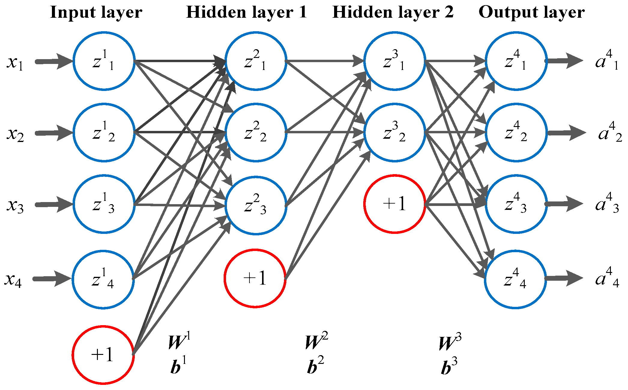
As mentioned above, ANN with symmetrical structure can be utilized for data compression and such special ANN is named as AE [35]. Figure 2 gives an AE with 4 input/output units and 2 hidden layers, where a^l_i is the activation (meaning output value) of unit i on layer l, z^l_i is the weighted sum of inputs to unit i on layer l including the bias term. W^l_ij is the weight associated with the connection between unit j on layer l and unit i on layer l+1. b^l_i is the bias associated with unit i on layer l. W^l and b^l are vector format of W^l_ij and b^l_i. Like other ANNs, to train an AE is to determine the weights of units. The optimization problem can be formulated as [36]:

$$\mathit{W}*,\mathit{b}*=\underset{\mathit{W},\mathit{b}}{\arg \min }L(\mathit{W},\mathit{b})=\underset{\mathit{W},\mathit{b}}{\arg \min }[\frac{1}{2N}{\displaystyle \sum _{j=1}^m{\displaystyle \sum _{i=1}^{n_1}{\left(a_{ij}^L-x_{ij}\right)}^2}}+\frac{\lambda }{2}\left({\displaystyle \sum _{l=1}^{L-1}{\displaystyle \sum _{j=1}^{n_l}{\displaystyle \sum _{i=1}^{n_{l+1}}{\left(W_{i,j}^l\right)}^2}}}\right)+\gamma {\displaystyle \sum _{l=2}^{L-1}{\displaystyle \sum _{i=1}^{N_l}KL(\delta ||{\delta }_i^l)}}]$$

(3)

where, m is the total number of load profiles, n is the number of data points in each profile. L is the number of layers. n^l is the total number of units on layer l except for the bias unit. λ and γ are weights of corresponding terms.

The first term in Equation (3) quantifies the error between the input and output load data. The second is a weight decay term used to prevent over-fitting. As mentioned above, the number of units on hidden layers determines the dimension of the compressed data, however, the regulating of hidden unit configuration is relatively not convenient. A sparsity constraint is introduced to compress the data volume adaptively, which is presented as the third term in Equation (3). For an ANN using sigmoid activation function, the unit is active when output approaches 1; oppositely, inactive when output approaches 0. The average activation level of hidden layers is imposed to approximate a small value, denoted as δ. The constraint of δ_i^l approaching δ can be achieved by the Kullback-Leibler divergence (KL-divergence).

$${\delta }_i^l=\frac{1}{m}{\displaystyle \sum _{j=1}^m{a}_{ij}^l}$$

(4)

$$\mathrm{KL}(\delta ||{\delta }_i^l)=\delta \log \frac{\delta }{{\delta }_i^l}+(1-\delta )\log \frac{1-\delta }{1-{\delta }_i^l}$$

(5)

KL-divergence is a standard function used to quantify the difference between two distributions [35]. When δ_i^l approaches δ, KL(δ||δ_i^l) approximates 0; when δ_i^l diverges from δ, KL(δ||δ_i^l) increases rapidly. Thus, minimizing this KL-divergence has the effect of forcing δ_i^l approaching δ.

Due to non-convexity, the minimum of the cost function cannot be solved by known closed-form ways. Iterative back propagation (BP) gradient algorithms are utilized to search the solutions [39], e.g., the Newton method, the gradient descent method, and the Limited-memory Broyden Fletcher Goldfarb Shanno (L-BFGS) algorithm [40]. The iterative ANN training is time-consuming compared with traditional methods such as PCA, DWT and SVD, which may be considered as a main limit for ANN-based load data compression.

The expression ability of any regression model is determined by the number of integrated variables. Therefore, for an ANN-based compressor, which is a non-linear regression essentially, its data compression effect is determined by the number of connecting weights. In order to compress the obtained load data to the desired sizes, the number of units on hidden layers must be decreased. If a very high CR is expected, the number of hidden units must be extremely small, in order to maintain the expression ability of the network (data recovery effect), the number of layers should be increased accordingly. Such networks with multiple hidden layers are called deep ANNs [35]. In other words, Deep ANNs actually use more longitudinal variables (layers) to reduce the horizontal variables (units). Due to the vanishing gradient [37], the training of deep networks is challenging for ANN-based data compression. In this paper, the utilized deep ANN is considered as a special network stacked by simple AEs, and a promising deep learning algorithm called wake-sleep [35] is introduced to solve the training problem, which will be illustrated in Section 6.

5. The Softmax Load Data Classifier

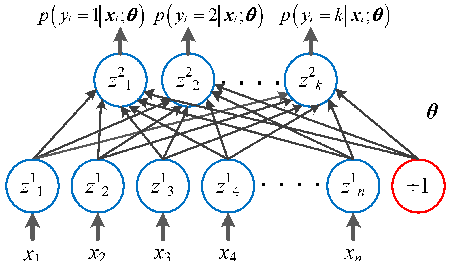
This section introduces a softmax load classifier. Shown in Figure 3, the softmax classifier is a simple ANN with only two layers, the input load data layer and the output label layer.

In this paper, the softmax regression is a supervised method used for multi-class load classification. To describe this in a probabilistic way, we want to estimate the probabilities of classifying the input load profile to each possible class and find the class with the maximum probability. Given an input x_i = (x_1i, x_2i, …, x_ni)^T, the label y_i can take k different values. Shown as Equation (4), the softmax classifier outputs a k dimensional vector (whose elements sum to 1) giving us k estimated probabilities [41].

$$h_{\mathit{\theta }}\left({\mathit{x}}_i\right)=\left[\begin{array}{c}p\left(y_i=1|{\mathit{x}}_i;\mathit{\theta }\right)\\ p\left(y_i=2|{\mathit{x}}_i;\mathit{\theta }\right)\\ ⋮\\ p\left(y_i=k|{\mathit{x}}_i;\mathit{\theta }\right)\end{array}\right]=\frac{1}{{\displaystyle \sum _{j=1}^k{e}^{{\mathit{\theta }}_j^T{\mathit{x}}_i}}}\left[\begin{array}{c}{e}^{{\mathit{\theta }}_1^T{\mathit{x}}_i}\\ e^{{\mathit{\theta }}_2^T{\mathit{x}}_i}\\ ⋮\\ e^{{\mathit{\theta }}_3^T{\mathit{x}}_i}\end{array}\right]$$

(6)

where θ₁, θ₂,…, θ_k∈R^k×1 are the classifier parameters to be trained. The probability of classifying x_i into category j is:

$$p\left(y_i=j|{\mathit{x}}_i;\mathit{\theta }\right)=\frac{e^{{\mathit{\theta }}_j^T{\mathit{x}}_i}}{{\displaystyle \sum _{l=1}^k{e}^{{\mathit{\theta }}_l^T{\mathit{x}}_i}}}$$

(7)

It worth noting that for supervised learning based on labeled data, the softmax output of the specific label dimension is imposed to be 1 and other dimensions are 0.

An indicator function ind{·} is adopted to formulate the cost function of softmax regression.

$$ind\{y_i=j\}=\{\begin{array}{c}1, if y=j\\ 0, if y\ne j\end{array}$$

(8)

Considering the factor of weight decay, the cost function and optimization problem of softmax regression can be expressed as [42]

$$\mathit{\theta }*=\underset{\mathit{\theta }}{\arg \min }J\left(\mathit{\theta }\right)=\underset{\mathit{\theta }}{\arg \min }\left(-\frac{1}{m}{\displaystyle \sum _{i=1}^m{\displaystyle \sum _{j=1}^{k}ind\left\{y_i=j\right\}}\log \frac{e^{{\mathit{\theta }}_j^T{x}_i}}{{\displaystyle \sum _{l=1}^k{e}^{{\mathit{\theta }}_l^T{x}_i}}}}+\frac{\lambda }{2}{\displaystyle \sum _{i=1}^k{\displaystyle \sum _{j=0}^n{\theta }_{ij}^2}}\right)$$

(9)

where, θ_ij is the weight of softmax classifier connecting unit j on input layer and unit i on output layer. In a similar way as AE, the softmax classifier can be trained by iterative BP algorithms.

6. Load Data Mining Based on Stacked Auto-Encoders

In this section, a deep ANN stacked by AEs is proposed for load data mining. As mentioned in the previous section, the proposed deep SAE is significantly more applicable to extract features and express data than basic AE.

The proposed network consists of L layers in which the outputs of below layers are connected to the inputs of the above layer. The lower part (layer 1 to L-1) is stacked by AEs, and the top layer (layer L) is a softmax classifier. As a typical deep ANN, the proposed network is difficult to train by the iterative BP algorithms due to gradient diffusion and a possible trap in local optima [37]. Therefore, a wake-sleep training principle of deep learning is introduced to train the network in the following two steps.

6.1. Wake Procedure: A Greedy Layer-Wise Pre-Training

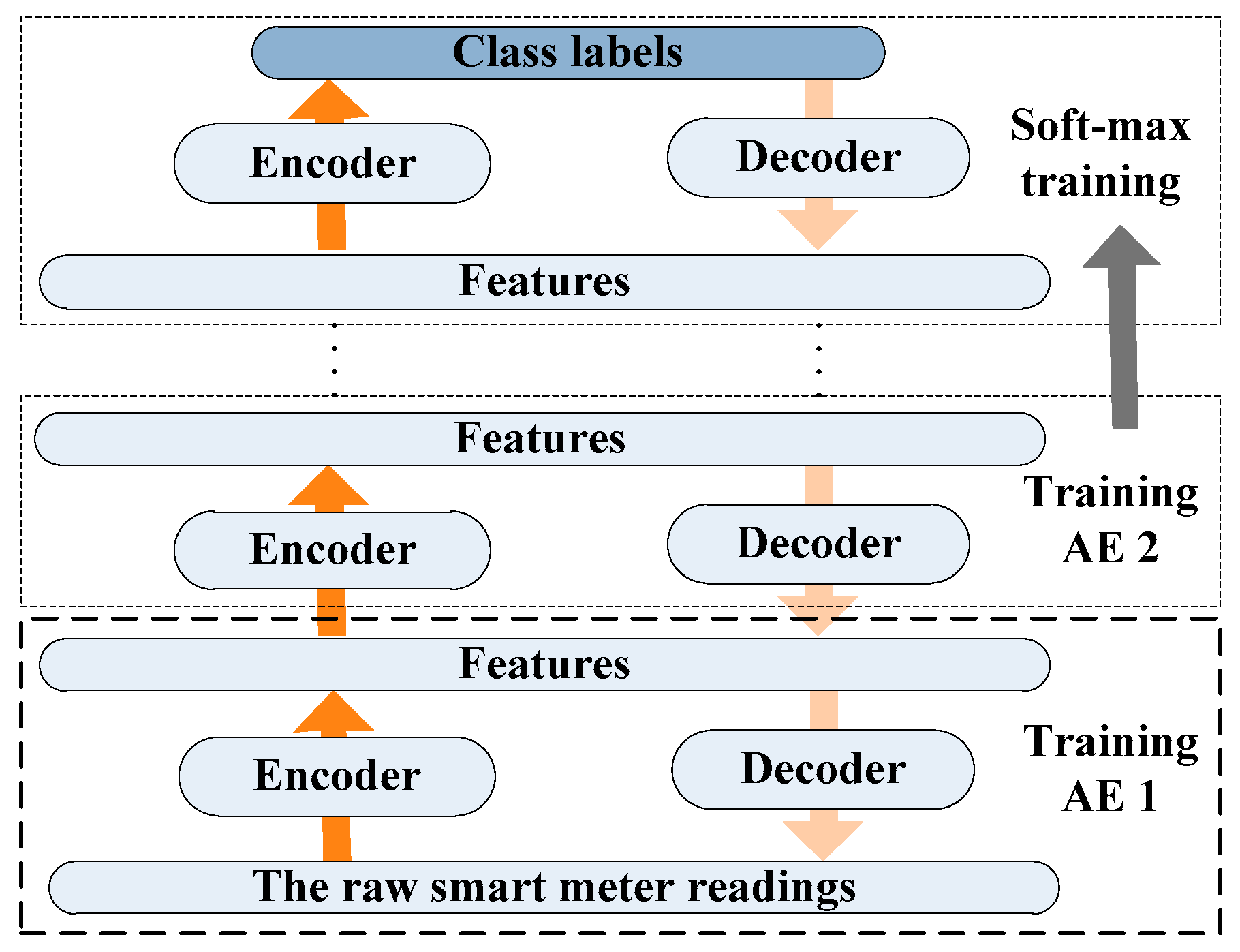
In this procedure, a greedy layer-wise training is performed, which consists of a layer-wise AE unsupervised self-learning and a supervised softmax regression [43,44].

Figure 4 illustrates the layer-wise training procedure. Specifically, in the stacked AE network, the decoding layers of AEs are implicit. As shown in Figure 4, if we supplement a decoding layer behind layer 2 to constitute a complete symmetric AE, we can train it through a self-learning algorithm. Expanding the same idea to layer l and (l + 1), the SAE can be trained in layer-wise way. Finally, a supervised softmax regression is performed on layer L. The detailed pseudo-codes of the wake step are given in

Table 1. Procedure of the greedy layer-wise training and fine-tuning.

Wake	(I) Unsupervised self-learning on SAE
	Start the training process Step1: Obtain a labeled dataset Ω(x, y). Randomize SAE and initialize the iterative counter l = 1, training set I = Ω(x). Step2: Connect a virtual decoding layer to layer (l+1) to form a symmetric AE, denoted as AE-l. Step3: Train AE-l with its input and output imposed equal to I using BP. Denote the weights of layer l as {Wl′, bl′}. Step4: Forward propagation to calculate the activations of layer (l+1), update I = a(l+1), l = l + 1. Step5: If l = L, then jump to Step 6, otherwise run back to Step2.
	(II) Supervised softmax regression
	Step6: Randomize the soft-max classifier weights θ. Input the activations of layer (L−1) to the classifier: zL = aL−1. Impose the label vector on the classifier output: aL = y. Step7: Train the classifier using BP to obtain the optimal weights, denoted as θ′.
Sleep	(III) Global fine-tuning on the whole ANN
	Step1: Randomize the whole ANN with the weights got in the wake step: W = Wl′, b = bl′, θ = θ′. Input the original dataset to the whole ANN: z1 = Ω(x). Impose the label vector on output: aL = y. Step2: Train the SAE and softmax classifier as a whole ANN using BP. Obtain the final optimal weights of all the layers, denoted as {W*,b*,θ*}. Terminate the training process

.

6.2. Sleep Procedure: A Global Fine-Tuning

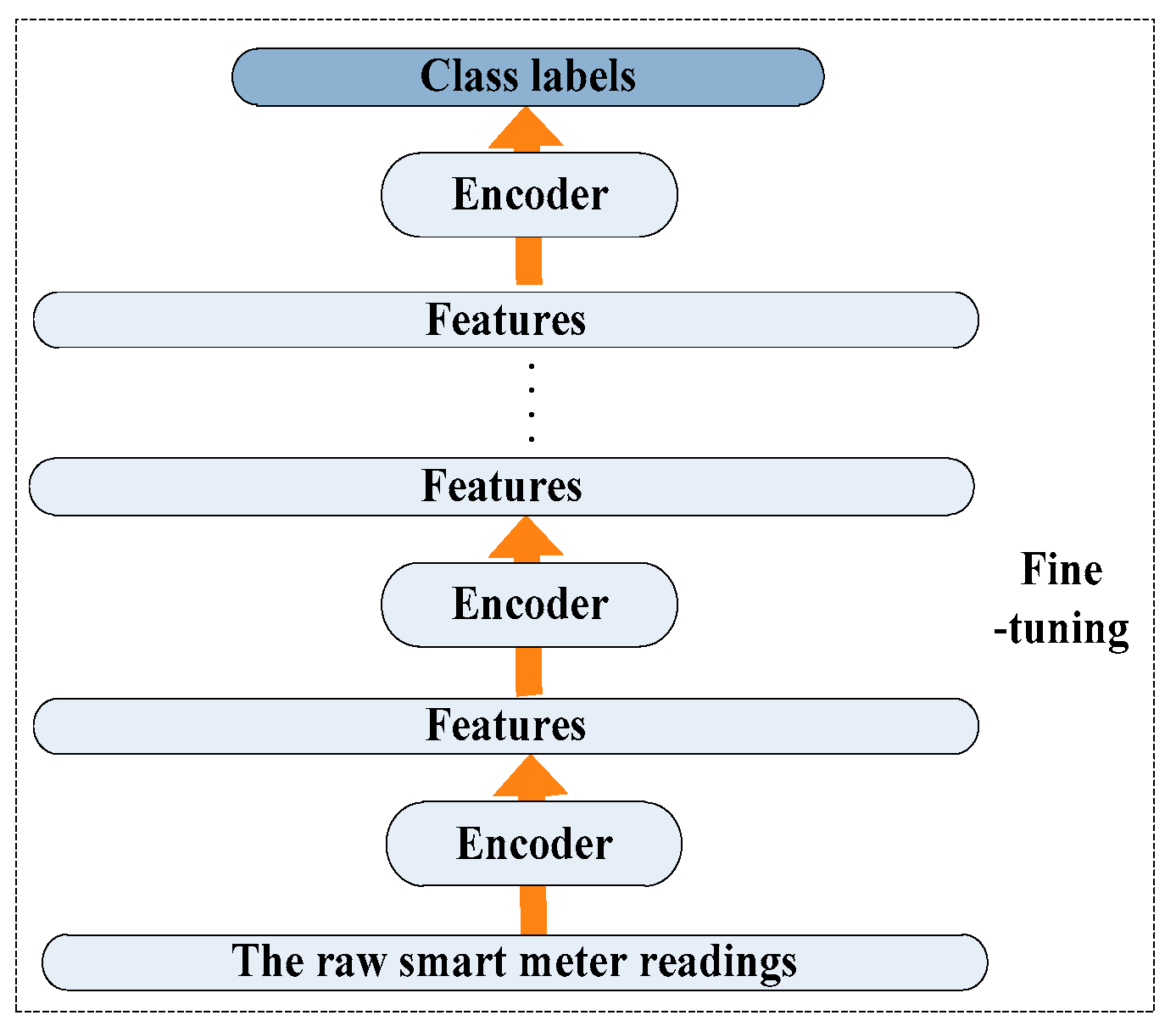
During the wake step, an initial setting of the weights is obtained by greedy layer-wise training. The next step is to further modify all the weights to minimize the error of the network as a whole. This is called the fine-tuning.

Figure 5 shows the fine-tuning procedure. In this step, we treat all layers, including AEs and the classifier, as a single integrated model. A supervised learning algorithm is utilized to fine-tune all the weights based on some labeled load data simultaneously. As the data is propagated from input to output, the error is transmitted down from the top. Pseudo-codes of the sleep algorithm can also be found in Table 1.

The ordinary BP ANNs are generally initialized randomly. For SAE, the initialization is done by a greedy layer-wise training, which makes the initial setting closer to the overall optima and helps to jump out of the local optima trap. Actually, the greedy layer-wise training is a pre-training, whose results are modified by fine-tuning in the next step [37]. The fine-tuning based on labeled load data is the most significant step for load data deep learning. The advantages of SAE for load data mining and the necessity of fine-tuning are demonstrated in the following case studies.

7. Case Studies

In this section, experiments on realistic datasets are used to demonstrate the feasibility of the proposed ANN based approach. Shown in

Table 2. Description of the utilized cases.

Case Name	Case1	Case2	Case3
Source	The EDAS of SGZEPC	The SEAI	Non- intrusive metering
Scenario	user segmentation		fault detection
Scale	house		appliance
Measure	power of user		current of fluorescent
Resolution	15 min	30 min	30 s
Dimension	daily(96)	daily(48)	hourly(120)
Training set	6000 single-peak commercial profiles, 4000 dual-peak industry profiles	50,000 residential profiles, 50,000 small & medium enterprise (SME) profiles	5000 normal profiles, 4000 abnormal profiles
Fine-tuning subset	500 commercial profiles, 400 industry profiles	5000 residential profiles, 5000 SME profiles	800 normal profiles, 800 fault profiles
Testing set	null	3000 residential profiles, 3000 SME profiles	200 normal profiles, 150 fault profiles
Label (y=)	1(commerce), 2(industry)	1(resident), 2(SME)	1 (normal), 2 (fault)

, three cases are utilized. Data of the case 1 are obtained through the Electric Data Acquire System (EDAS) of State Grid Zhejiang Elec. Power Corp. (SGZEPC) in China. Case 2 is provided by the Sustainable Energy Authority of Ireland (SEAI). Case 3 contains accumulated measurements in our lab. The main parameters of are given in

Table 3. Parameters setting of AE in this paper.

Parameter	δ	λ	γ	optimization algorithm
Value	0.1	0.003	3	L-BFGS

[35]. Due to the page limitation, the sensitivity analysis of these parameters is omitted here.

In this section, SAE (n₁/n₂,…, N) denotes a SAE network with n₁ units on layer 1, n₂ units on layer 2, et al. Here, N is the iteration number of BP training. Equally, AE (n₁/n₂, N) denotes a basic AE with n₁ and n₂ units on layer 1 and 2, respectively.

7.1. Performance of Basic AE

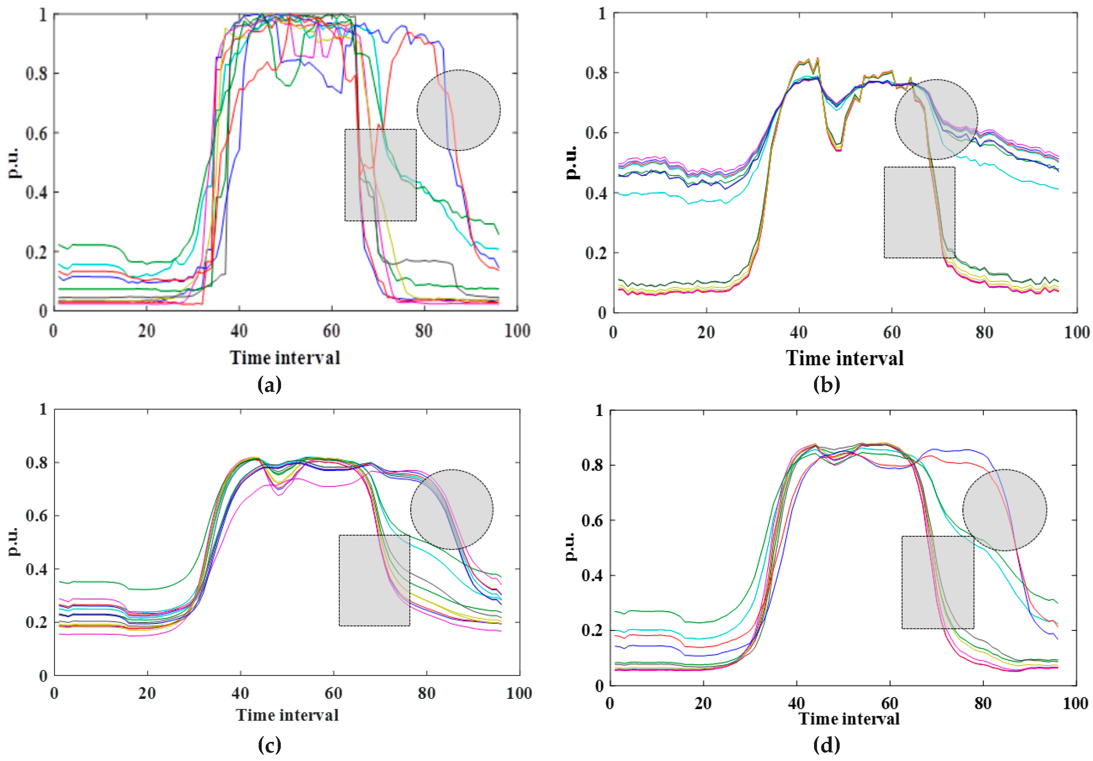
Ten thousand 96-dimension representative daily profiles in Case1 are compressed. Due to page limitation, the samples are ordered in terms of electricity consumption or transformer capacity from highest to lowest, and then the profiles of top 15 users are selected to be displayed. Figure 6 displays the original normalized profiles, as well as the reconstructed ones by different AEs. As can be seen, AE (96/20,50), AE(96/5,900), and AE(96/20,900) all recover the basic profiles. The performance of AE (96/20,900) is better than AE(96/20,50) and AE(96/5,900). This can be demonstrated in the following aspects:

(1)

The range of the reconstructed profiles of AE(96/5,900) and AE(96/20,900) are [0.15,0.8] and [0.05,0.89] respectively. While, several reconstructed profiles of AE(96/20,50) are narrowed to [0.4,0.8]. AE(96/20,900) fits the original data range [0,1] better obviously.

(2)

Focus on the shaded circular areas in Figure 6, AE(96/20,900) successfully recovers the paths of the profiles, including their overlap, while AE(96/20,50) and AE(96/5,900) both distorts severely in this area.

(3)

Focus on the shaded rectangular areas in Figure 6, AE(96/20,900) recovers the similar steep extent of original profile, while the profiles of AE(96/20,50) and AE(96/5,900) are obviously more placid than the original one in this area.

Based on the different reconstruction results of AE(96/20,50), AE(96/5,900), and AE(96/20,900), we can preliminarily conclude that the load data compression performance of AE is determined by the number of iterations and features (number of hidden units).

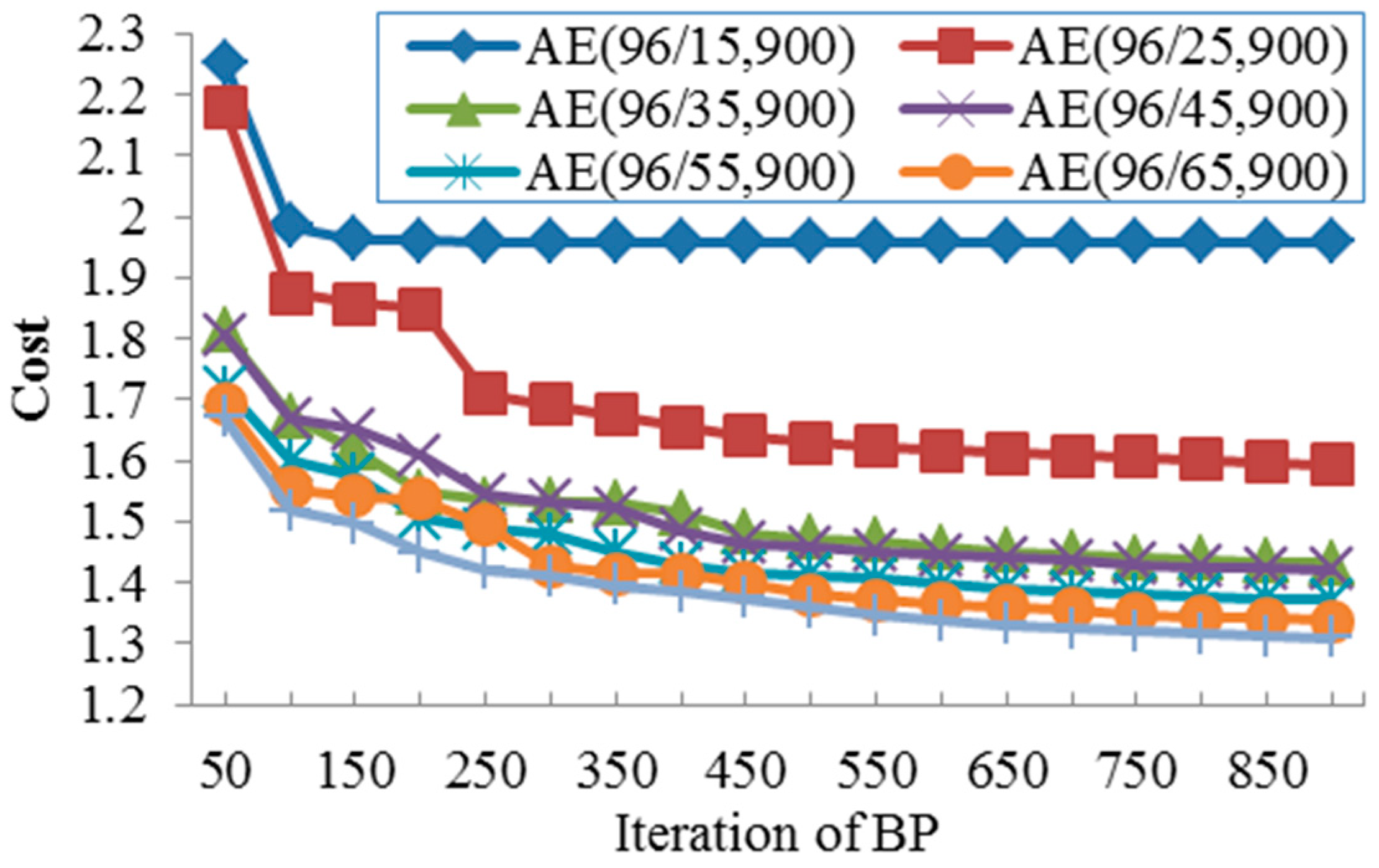
Figure 7 further illustrates the relationship of the cost, features, and iterations of BP. The indicated results are summarized as follows:

With the increasing of hidden units, the minimum cost decreases but the decreasing speed slows down. As can be seen, the gap between AE(96/75) and AE(96/65) is obviously smaller than the that between AE(96/15) and AE(96/25). As hidden units correspond to features, this indicates that an evident redundancy exists in load data. For instance, encoded in 45 features, the load data can be decoded well with a small cost below 1.4. Figure 7 also indicates a proper maximum iteration, over which, more BP iterations produce little effects. In Figure 7, if 15 features are used, 150 iterations are enough; when 45 features are used, 500 iterations are appropriate.

7.2. Performance of SAE

Figure 8 displays the features of three representative profiles (L1, L2, and L3) obtained on different hidden layers of SAE (96/48/24/12,500). The dataset is case1. Visually, the 96 load points recovered from 6 features are close to the original data. The recovering performance is much better that that of basic AE in Figure 6.

It can be seen from Figure 8 that the hidden layers express the data based on pulse signals with fewer dimensions. Specifically, different pulse shapes (triangle or trapezoid), pulse numbers, pulse permutations can distinguish different types of input load. These are high-order descriptions of load data based on extracted features.

A message from Figure 8 is that some tiny differences can also be observed with high order features. For example, on hidden layer 4 where loads are expressed in 6 features very concisely, the different electricity consumption characteristics of the three profiles are displayed intuitively. Specifically, profile 1 and 2 are exactly the same in 4 features (feature 1, 3, 4, and 6), while L1 and L3 are only consistent in 2 features (feature 2 and 5). From the perspective of original data, L1 and L2 are both in single-peak shape, while profile 3 presents dual peaks.

If L1, L2, and L3 are representative profiles of three users and this is a user segmentation problem, then user 1 and 2 are more likely to be put into the same class while user 3 should be isolated. If the three profiles are metered from the same user for abnormal detecting, then profile 3 should be determined as an event profile of abnormal behavior. Obviously, the high order features grasp the essential characteristic of input and are of great significance for the understanding of data.

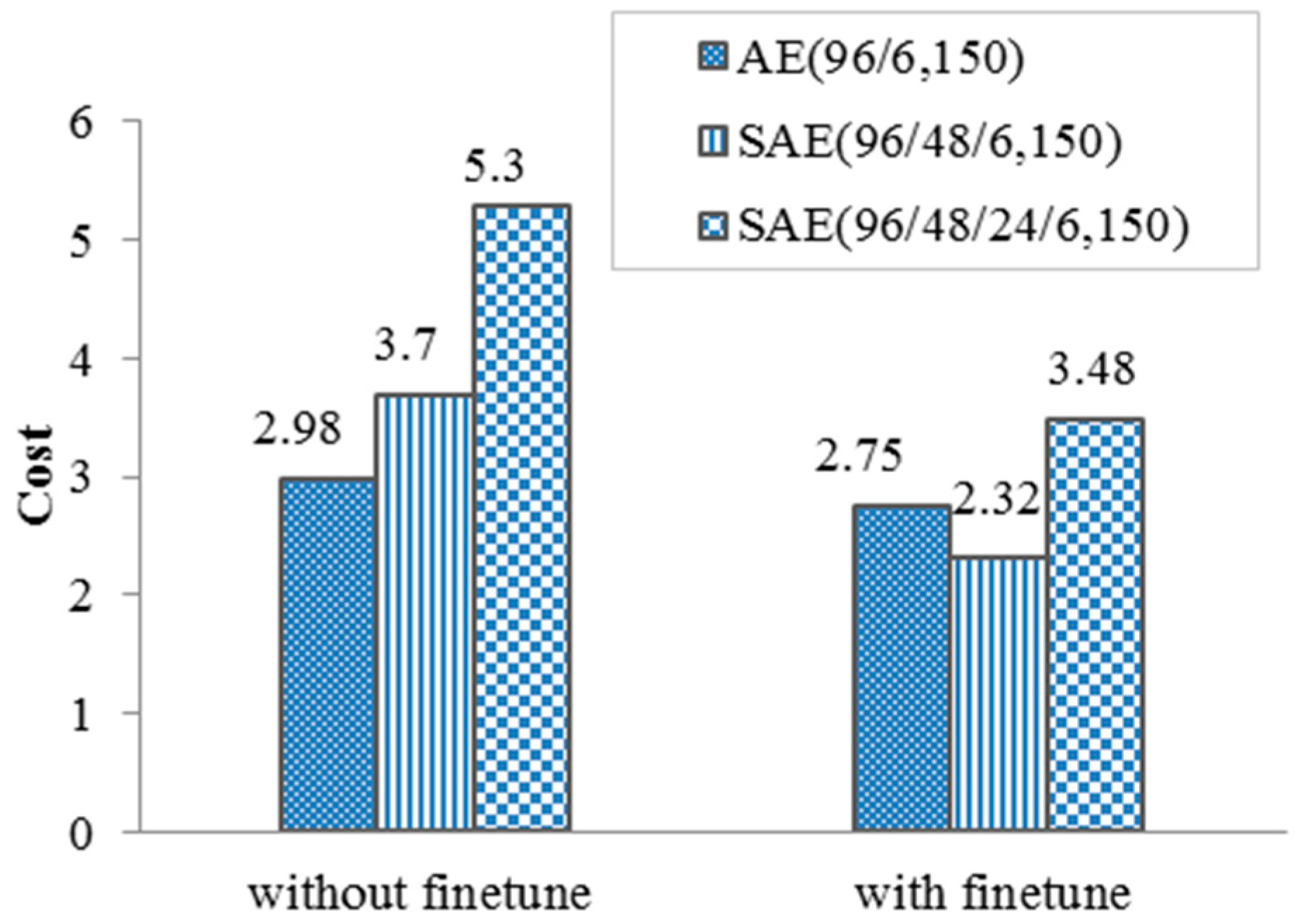
It is worth noting that an obvious information distortion exists in the shaded circular area. Through, the objective of SAE is to restore the input as much as possible, error generates in the layer-wise self-learning due to local optima trap or other factors, which gradually enlarges with the layer-wise greedy training from the lower to the top AE. Considering the multiple layers, the error of SAE is usually large than single AE. It is not hard to imagine that some dual-peak profiles may be smoothed to be single-peak and misclassified on top layers (refer to the red profile in Figure 6a,d). As mentioned above, well-defined labeled data can be utilized to fine tune the network and help decrease the error. In case 1, the labels are determined on profile shape, 1 for single-peak and 2 for dual-peak. Figure 9 displays the compression costs of different SAEs with and without fine-tuning performed.

As can be seen from Figure 9, error of the three networks both decrease after fine-tuning based on well-defined labeled data. It is also demonstrated that a relatively appropriate depth (number of layers) exists for a given dataset. In case 1, the SAE including two hidden layers with fine-tuning achieves the minimum cost, which is 2.32. The increase of depth from 2 to 3 produces no improvement and brings some negative effect.

Lossy compression is essentially a tradeoff between data volume and error. From this perspective, two indexes are introduced including CR and the Root Mean Square Error (RMSE) [7]. CR is the ratio between the sizes of the original and compressed data, RMSE is a widely used measure of the reconstruction error. For ANN based load data compression, CR is determined by the number of output units, e.g., AE (96/48) gives a CR of 2.

In terms of CR and RMSE, the compression performances of SAE (with fine-tuning) and several other methods are compared on case 1, including PCA [24], DWT [25,26] and k-SVD [7,21]. Figure 10 displays the results. As can be seen, the RMSE of SAE grows very slowly with the increasing CR. SAE achieves relatively lower RMSE values than the other linear methods at given CRs. If the load data is compressed to 1/16 of its original size, the corresponding RMSE of SAE is only 0.092, which is greatly lower than k-SVD (0.16), DWT (0.24) and PCA (0.27).

To obtain a higher CR, fewer units should be deployed on the output layer, but we can still control the RMSE by increasing the hidden layers and fine-tune the whole network based on high quality labeled data. This is a significant advantage of ANN-based compressor.

7.3. Accuracy of the Proposed Classifier

Case 2 and 3 in Table 2 are utilized to show the effects of using SAE and softmax regression for load data classification.

Confusion matrixes [9] of the case 2 are illustrated in

Table 4. Confusion matrix of case 2.

Label		Actual
		SME	Resident
Predicted	SME	ss	sr
	resident	rs	rr

. Variable ss and sr denote the number of SMEs correctly predicted as SMEs, incorrectly predicted as residents respectively. Similarly, all the other variables in

Table 5. The classification accuracy of different algorithms.

Algorithm			ac (%)
Compression		Classifier	Case 2	Case 3
AE (x/25,500)	fine-tuning	softmax	89.18	93.92
	no fine-tuning		77	81.64
SAE (x/40/15,500)	fine-tuning	softmax	91.64	97.31
	no fine-tuning		75.92	76.72
null		softmax	73.95	75.90
null		SVM [7]	73.66	78.10
k-SVD [7]		SVM [7]	87.70	91.96
DWT [25]		SVM [7]	74.20	79.31
PCA [24]		SVM [7]	74.63	82.63

can be defined. Then, the classification accuracy index a_c is introduced to evaluate the performance of classifier. a_c is formulated as the proportion of the samples that are correctly classified in the whole set.

$$a_c=\frac{ss+rr}{sr+rs+ss+rr}\times 100\%$$

(10)

In the similar way, a_c index of case 3 can also be defined. Table 5 illustrates the numerical comparison of the proposed method and some state-of-the-art load data classification models, the following results can be summarized:

(a)

Indicated by the different a_c values of softmax and “AE+softmax,” extracted features help improve the classification accuracy.

(b)

Fine-tuning is necessary for SAE training, which greatly improves the accuracy by over 10 percentages.

(c)

Compared ac values of AE(x/25,500) and SAE(x/40/15, 500), features extracted in layer-wise way helps improve the classification. The premise is the adopted fine-tuning.

(d)

With fine-tuned SAE, more than 97% fault events are correctly detected and over 90% SMEs and residents are correctly classified. Such a high accuracy may not be achieved by common “linear compressor + classifier” models.

8. Conclusions

In this paper, an ANN based smart meter data mining approach is exploited. First, to satisfy the bandwidth constraint for signal transmission and space requirement for data storage, an innovative framework for smart meter data flow is established. Specifically, SAEs are installed at the user side to compress the meter readings. The corresponding decoding network is preconfigured in the data center, which can recover the compressed data if needed. Compared to the existing linear models such as PCA, DWT, and SVD, the proposed SAE compressor is of higher CRs with satisfactory errors. For advanced demand side applications, a labeled data driven strategy for accuracy improvement of unlabeled data classification is invented. Specifically, massive unlabeled data are classified by softmax classifier in data center based on features extracted by remote SAEs. A following-up training is implemented to fine-tune the weights after pre-training. It is demonstrated by the numerical results that the fine-tuning based on well-defined labeled dataset greatly modifies the extracted high order features and improves the accuracy.

Moreover, the iterative gradient descent calculation is the most time-consuming step, and the massive sample data and their intermediate calculation quantities are the main memory overhead for the proposed method, which both occur in the training step and can be completed in the manufacturing or debugging stage of smart meters. Thus, by integrating pre-trained networks into smart meters, the proposed method is feasible to handle the curse of CPU time and memory.

The proposed method has a significantly fit for both building level user segmentation and appliance level event detection. It is a feasible tool to deal with big data on demand side, which has a convincing application potential in power billing, demand response, and load forecasting.

References

- Katiraei, F.; Iravani, M.R. Power management strategies for a microgrid with multiple distributed generation units. IEEE Trans. Power Syst. 2006, 21, 1821–1831. [Google Scholar] [CrossRef]
- Peppanen, J.; Reno, M.J.; Thakkar, M.; Grijalva, S.; Harley, R.G. Leveraging AMI data for distribution system model calibration and situational Awareness. IEEE Trans. Smart Grid 2015, 6, 2050–2059. [Google Scholar] [CrossRef]
- Akkaya, K.; Rabieh, K.; Mahmoud, M.; Tonyali, S. Customized certificate revocation lists for IEEE 802.11s-based smart grid AMI networks. IEEE Trans. Smart Grid 2015, 6, 2366–2374. [Google Scholar] [CrossRef]
- Department for Business Energy and Industrial Strategy. Smart Meters, Quarterly Report to End December 2016; Technical Report; Department for Business Energy and Industrial Strategy: Great Britain, UK, 2017.
- Adam Cooper. Electric Company Smart Meter Deployments: Foundation for a Smart Grid; Technical Report; The Edison Foundation: Washington, DC, USA, 2016. [Google Scholar]
- Abuadbba, A.; Khalil, I.; Yu, X. Gaussian approximation-based lossless compression of smart meter readings. IEEE Trans. Smart Grid 2018, 9, 5047–5055. [Google Scholar] [CrossRef]
- Wang, Y.; Chen, Q.X.; Kang, C.Q.; Xia, Q. Sparse and redundant representation-based smart meter data compression and pattern extraction. IEEE Trans. Power Syst. 2017, 32, 2142–2151. [Google Scholar] [CrossRef]
- Ye, C.J.; Ding, Y.; Song, Y.H.; Lin, Z.Z.; Wang, L. A data driven multi-state model for distribution system flexible planning utilizing hierarchical parallel computing. Appl. Energy 2018, 232, 9–25. [Google Scholar] [CrossRef]
- Wang, Y.; Chen, Q.X.; Kang, C.Q.; Xia, Q. Clustering of electricity consumption behavior dynamics toward big data application. IEEE Trans. Smart Grid 2016, 7, 2437–2447. [Google Scholar] [CrossRef]
- D2-21 CIGRE Working Group D2.21, WG. Broadband PLC Applications. CIGRE, June 2008. Available online: http://www.cigre.org/What-is-CIGRE (accessed on 5 January 2019).
- Wang, Y.; Chen, Q.X.; Kang, C.Q. Load profiling and its application to demand response: A review. Tsinghua Sci. Technol. 2015, 20, 117–129. [Google Scholar] [CrossRef]
- Quilumba, F.L.; Lee, W.; Huang, H. Using smart meter data to improve the accuracy of intraday load forecasting considering customer behavior similarities. IEEE Trans. Smart Grid 2015, 6, 911–918. [Google Scholar] [CrossRef]
- Wang, Y.; Chen, Q.X.; Hong, T.; Kang, C.Q. Review of smart meter data analytics: Applications, methodologies, and challenges. IEEE Trans. Smart Grid Early Access 2018. [Google Scholar] [CrossRef]
- Gerek, O.N.; Ece, D.G. Compression of power quality event data using 2d representation. Electr. Power Syst. Res. 2008, 78, 1047–1052. [Google Scholar] [CrossRef]
- Tate, J.E. Preprocessing and Golomb-Rice encoding for lossless compression of phasor angle data. IEEE Trans. Smart Grid 2016, 7, 718–729. [Google Scholar] [CrossRef]
- Unterweger, A.; Engel, D. Resumable load data compression in smart grids. IEEE Trans. Smart Grid 2015, 6, 919–929. [Google Scholar] [CrossRef]
- Ringwelski, M.; Renner, C.; Reinhardt, A.; Weigel, A.; Turau, V. The hitchhiker’s guide to choosing the compression algorithm for your smart meter data. In Proceedings of the 2nd Energy Conference & Exhibition, Florence, Italy, 9–12 September 2012; pp. 935–940. [Google Scholar]
- Notaristefano, A.; Chicco, G.; Piglione, F. Data size reduction with symbolic aggregate approximation for electrical load pattern grouping. IET Gener. Transm. Distrib. 2013, 7, 108–117. [Google Scholar] [CrossRef]
- Tong, X.; Kang, C.Q.; Xia, Q. Smart metering load data compression based on load feature identification. IEEE Trans. Smart Grid 2016, 7, 2414–2422. [Google Scholar] [CrossRef]
- Tripathi, S.; De, S. An efficient data characterization and reduction scheme for smart metering infrastructure. IEEE Trans. Ind. Inform. 2018, 14, 4300–4308. [Google Scholar] [CrossRef]
- Souza, J.C.S.D.; Assis, T.M.L.; Pal, B.C. Data compression in smart distribution systems via singular value decomposition. IEEE Trans. Smart Grid 2017, 8, 275–284. [Google Scholar] [CrossRef]
- Li, R.; Li, F.R.; Smith, N.D. Load characterization and low-order approximation for smart metering data in the spectral domain. IEEE Trans. Ind. Inform. 2017, 13, 976–984. [Google Scholar] [CrossRef]
- Khan, J.; Bhuiyan, S.; Murphy, G.; Williams, J. The compression of electric signal waveforms for smart grids: State of the art and future trends. IEEE Trans. Smart Grid 2014, 5, 291–302. [Google Scholar]
- Ahmadi, H.; Martí, J.R. Load decomposition at smart meters level using eigenloads approach. IEEE Trans. Power Syst. 2015, 30, 3425–3436. [Google Scholar] [CrossRef]
- Tse, N.C.F.; Chan, J.Y.C.; Lau, W.H.; Poon, J.T.Y.; Lai, L.L. Real-time power-quality monitoring with hybrid sinusoidal and lifting wavelet compression algorithm. IEEE Trans. Power Deliv. 2012, 27, 1718–1726. [Google Scholar] [CrossRef]
- Rana, M.; Koprinska, I. Forecasting electricity load with advanced wavelet neural networks. Neurocomputing 2006, 182, 118–132. [Google Scholar] [CrossRef]
- Zhong, S.; Tam, K.S. Hierarchical classification of load profiles based on their characteristic attributes in frequency domain. IEEE Trans. Power Syst. 2015, 30, 2434–2441. [Google Scholar] [CrossRef]
- Chicco, G.; Napoli, R.; Piglione, F. Comparisons among clustering techniques for electricity customer classification. IEEE Trans. Power Syst. 2006, 21, 933–940. [Google Scholar] [CrossRef]
- Carpinteiro, O.A.; Da Silva, A.P. A hierarchical self-organizing map model in short-term load forecasting. J. Intell. Robot. Syst. 2001, 31, 105–113. [Google Scholar]
- Lu, C.N.; Wu, H.T.; Vemuri, S. Neural network based short term load forecasting. IEEE Trans. Power Syst. 2002, 8, 336–342. [Google Scholar] [CrossRef]
- Guo, Z.Y.; Wang, Z.J.; Kashani, A. Home appliance load modeling from aggregated smart meter data. IEEE Trans. Power Syst. 2015, 30, 254–262. [Google Scholar] [CrossRef]
- Guo, K.Y.; Sui, L.Z.; Qiu, J.T.; Yu, J.C.; Wang, J.; Yao, S.; Han, S.; Wang, Y.; Yang, H. Angel-Eye: A Complete Design Flow for Mapping CNN onto Embedded FPGA. IEEE Trans. Comput.-Aided Des. Integr. Circuits Syst. 2018, 37, 35–47. [Google Scholar] [CrossRef]
- Montalvo, A.J.; Gyurcsik, R.S.; Paulos, J.J. Toward a general-purpose analog VLSI neural network with on-chip learning. IEEE Trans. Neural Netw. 1997, 8, 413–423. [Google Scholar] [CrossRef]
- Kim, N.; Kehtarnavaz, N.; Yeary, M.B.; Thornton, S. DSP-based hierarchical neural network modulation signal classification. IEEE Trans. Neural Netw. 2003, 14, 1065–1071. [Google Scholar]
- UFLDL Tutorial. Available online: http://deeplearning.stanford.edu/wiki/index.php/UFLDL_Tutorial (accessed on 18 February 2019).
- Yu, C.N.; Mirowski, P.; Ho, T.K. A sparse coding approach to household electricity demand forecasting in smart grids. IEEE Trans. Smart Grid 2017, 8, 738–748. [Google Scholar] [CrossRef]
- Hinton, G.E.; Salakhutdinov, R.R. Reducing the dimensionality of data with neural networks. Science 2006, 313, 504–507. [Google Scholar] [CrossRef] [PubMed]
- Ye, C.J.; Huang, M.X. Multi-objective optimal power flow considering transient stability based on parallel NSGA-II. IEEE Trans. Power Syst. 2015, 30, 857–866. [Google Scholar] [CrossRef]
- Goodfellow, I.; Bengio, Y.; Courville, A. Deep Learning; MIT Press: Cambridge, MA, USA, 2016. [Google Scholar]
- Nocedal, J. L-BFGS: Software for Large-Scale Unconstrained Optimization. Available online: http://users.iems.northwestern.edu/~nocedal/lbfgs.html (accessed on 18 February 2019).
- Sutton, R.; Barto, A. Reinforcement Learning: An Introduction; MIT Press: Cambridge, MA, USA, 1998. [Google Scholar]
- Bishop, C.M. Pattern Recognition and Machine Learning; Springer: New York, NY, USA, 2006. [Google Scholar]
- Hinton, G.E.; Osindero, S.; Teh, Y. A fast learning algorithm for deep belief nets. Neural Comput. 2006, 18, 1527–1554. [Google Scholar] [CrossRef] [PubMed]
- Bengio, Y.; Lamblin, P.; Popovici, D.; Larochelle, H. Greedy layer-wise training of deep networks. In Advances in Neural Information Processing Systems 19 (NIPS‘06); MIT Press: Cambridge, MA, USA, 2007; pp. 153–160. [Google Scholar]
Figure 1.
Framework of the proposed Artificial Neural Network (ANN)-based model.
Figure 2.
Topology structure of a simple Auto-Encoder (AE).
Figure 3.
Topology of a simple softmax classifier.
Figure 4.
The greedy layer-wise training.
Figure 5.
The overall fine-tuning.
Figure 6.
(a) Original 15 load profiles in case1; (b) Reconstructed load profiles by AE(96/20,50); (c) Reconstructed load profiles by AE(96/5,900); (d) Reconstructed load profiles by AE(96/20,900).
Figure 7.
Relationship of the cost, features, and iterations.
Figure 8.
Features extracted on different hidden units of stacked auto-encoder (SAE) (96/48/24/12,500).
Figure 9.
The compression costs of different SAEs on case 1.
Figure 10.
Comparison of SAE and linear algorithms.