Global Maximum Power Point Tracking under Shading Condition and Hotspot Detection Algorithms for Photovoltaic Systems


1
Graduate School of Engineering and Science, Shibaura Institute of Technology, Tokyo 135-8548, Japan
2
Department of Electrical Engineering, Shibaura Institute of Technology, Tokyo 135-8548, Japan
*
Author to whom correspondence should be addressed.
Energies 2019, 12(5), 882; https://doi.org/10.3390/en12050882
Submission received: 10 January 2019
/
Revised: 22 February 2019
/
Accepted: 24 February 2019
/
Published: 7 March 2019
(This article belongs to the Special Issue Advances in Electrical Power Engineering—Select papers from 53rd International Universities Power Engineering Conference (UPEC2018))
Abstract
:Photovoltaic (PV) technology has been gaining an increasing amount of attention as a renewable energy source. Irradiation and temperature are the two main factors which impact on PV system performance. When partial shading from the surroundings occurs, its incident shadow diminishes the irradiation and reduces the generated power. Moreover, shading affects the pattern of the power–voltage (P–V) characteristic curve to contain more than one power peak, causing difficulties when developing maximum power point tracking. Consequently, shading leads to a hotspot in which spreading the hotspot widely on the PV panel’s surface increases the heat and causes damage to the panel. Since it is not possible to access the circuit inside the PV cells, indirect measurement and fault detection methods are needed to perform them. This paper proposes the global maximum power point tracking method, including the shading detection and tracking algorithm, using the trend of slopes from each section of the curve. The effectiveness was confirmed from the dynamic short-term testing and real weather data. The hotspot-detecting algorithm is also proposed from the analysis of different PV arrays’ configuration, which is approved by the simulation’s result. Each algorithm is presented using the full mathematical equations and flowcharts. Results from the simulation show the accurate tracking result along with the fast-tracking response. The simulation also confirms the success of the proposed hotspot-detection algorithm, confirmed by the graphical and numerical results.
1. Introduction
The issues of energy crisis and environmental concern have gained much attention throughout this recent period. Research in renewable energy has particularly garnered a lot of attention, especially for Photovoltaic (PV) technology [1]. In regard to enhancing the performance of the PV system, two main factors have an impact on PV power generation—the irradiation and temperature [2]. It is apparent that we cannot control these factors due to the location dependency; therefore, the problem of “PV mismatch” happens. Defined by Gosumbonggot [3], PV mismatch is described as the difference between the expected and actual output power from a PV module, which causes difficulties to PV for generating the power. In this paper, shading mismatch is the primary consideration. The effect originates from several environmental factors, especially the shade from buildings, clouds, trees, and PV panel alignment in the solar farm. It is explained by many types of research, where it is said that shading contributes to the obstacle for PV power generation, and is observed from numerous installed PV systems around the world [4,5]. There has previously been an example from the PV rooftop systems in Germany, where 41% of the installed panels were affected by shading, and the energy losses were up to 10%. Hence, a remarkable reduction of power generated is observed [6]. Similarly, Daraban et al. [7] presented a case study where 13 different PV power tracking systems operated under shading conditions, where the result was that up to 70% of power was lost due to the actual maximum power being undetected.
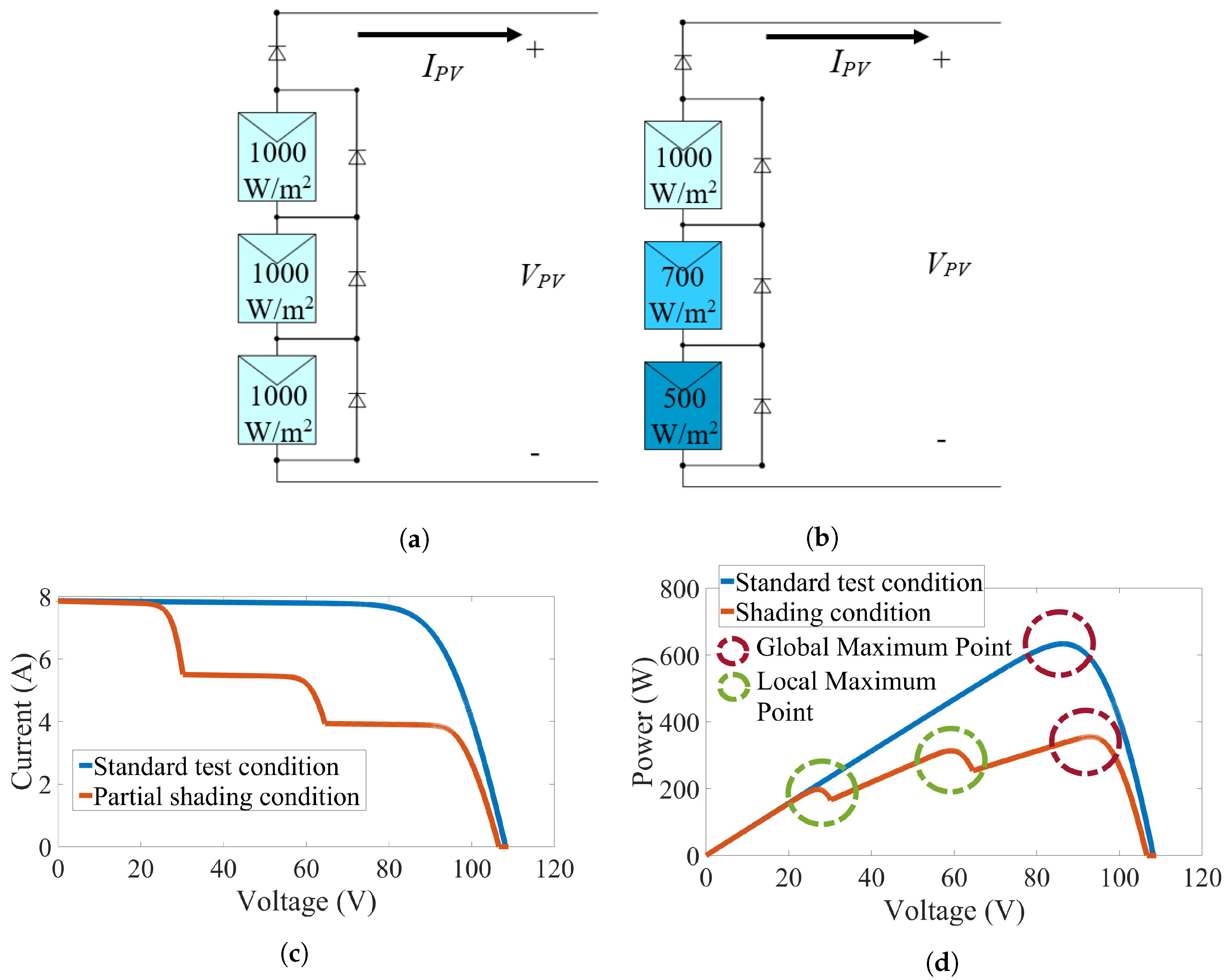
In order to observe how shading behavior affected the PV’s performance, a basic simulation was performed. Figure 1a,b presents the series-connected PV array circuit operated at the standard test condition (STC) and partial shading, respectively. In the circuit, the bypass and blocking diodes are installed on each PV branch, which is the usual manner when installing the PV system [2,8,9]. Figure 1c,d shows how the current–voltage (I–V), and power–voltage (P–V) characteristic curve corresponds to each condition. From both curves, the significant difference between the two conditions can be observed, especially in the P–V curve. Shading affects the pattern of the curves and exhibits multiple local peaks, while the normal condition shows only a single peak. Naming each peak as the local power peaks, with the highest among all points being the global power peak, increases the challenge for the maximum power point tracking (MPPT) system to locate the correct global power peak point [2,10,11,12].
It has been confirmed by previous research that the conventional MPPT methods fail to ensure successful and precise tracking of global power peaks under the shading condition [7,10,11,12,13]. Hence, there are many proposed MPPT techniques. The techniques can be grouped into two categories, differentiated from the method of implementation. The first category originates from the improvement of the existing conventional tracking method, including the well-known MPPT techniques but with further modification (e.g., the perturb and observed (P&O) and the incremental conductance (InC), where the results also confirmed their effectiveness [14,15,16,17,18]). The second category is the topologies based on the intelligence computing method. Examples include the fuzzy logic-based MPPT, artificial neural network (ANN), and artificial bee colony presented by Bidyadhar et al. [19] and Kinattigal et al. [20]. Consequently, the difficulties for implementing MPPT include the complexity of the algorithm, cost, and failure while operating in the shading condition [6]. In particular, studies of the global power peak identification under the shading condition have been carried out a lot in the last five years, where each study presented a tracking method with various forms of complexity, cost, operating speed, and range of effectiveness [13]. These variations should be taken into consideration when designing an effective MPPT system [5]. Much research has also proposed interesting ideas for implementing MPPT [5,6,15,17,18], and has proved its effectiveness. However, its major disadvantages are the requirements of samples, the additional control circuit, complicated implementation, and tracking time consumption. Further, the long-term testing has not been presented. Furthermore, research developed by Kobayashi et al. [21] and Irisawa et al. [22] shows the simplification from the complex MPPT system, called the two-stage maximum power point tracking control. Nonetheless, studies which still address the problem faced when operating under some non-uniform irradiation conditions and the additional control circuit is also required.
As for other intelligence tracking methods proposed in many research papers, they show the guarantee of tracking MPPT in the shading condition. Nonetheless, the significant disadvantages of the intelligence technique is the requirement of additional circuits, greater complexity, and high implementation costs [5,23]. For instance, the proposed adaptive inertial weight particle swarm optimization (AWIPSO) was implemented based on the original particle swarm optimization (PSO) method [24]. The work establishes a decrease in tracking time; however, the experimental result is not shown in this paper. The complexity of intelligence methods is presented in References [11,25]. The methods not only require the calculation for related variables, but precision in setting, and the requirement of cooperative agents and learning factors are also necessary. Apart from PSO, Alajmi et al. [26] presented a modified fuzzy-logic controller. The design is based on the diode model equation of the PV panel, combined with the modified fuzzy-logic from the hill-climbing method. However, the system requires thirty-two fuzzy control rules, which brings more complexity to the system.
In a practical case, the PV inverter is one of the necessary equipments for PV installation. Most of the commercial inverters have the MPPT program embedded, based on scanning P&O and the InC algorithm [11]. From the technical specification of PV inverters, scanning is set to be every 15 min of the time interval [27,28]. Therefore, the weakness of this topology is the mismatch of the tracking interval with the weather condition [3]. By choosing a long scanning interval on days with rapid change of weather, tracking errors may occur due to the mismatch of the selected range. Further, when choosing a short scanning interval on days with a steady change of irradiation and temperature, power loss from the unnecessary tracking can occur [29]. Although the system includes blocking and bypass diodes to prevent heating and damage, considerable decrease in power from shading can still happen.
As a consequence, if shading occurs to the PV panel, it can lead to a fault called the hotspot. The hotspot is one of the frequently occurring faults for the PV panel, which happens when the cell is entirely or partially shaded, cracked, or electrically mismatched. Research by Pillai and Rajasekar [8] describes the damage from the hotspot towards the solar farm in the US and shows that hotspots can cause a reduction of energy yields up to 6%. Furthermore, degradation of the panel will increase over the operating time, and the hotspot will continue to heat up and thus result in more physical damage to the modules. Evidence of this is shown in Reference [30], which says that the degradation rate of the hotspot PV module appears to degrade at a higher rate than the non-hotspot modules, which could lead to module mismatch issues in a module-string. The rate for 12-year modules varies between 0.6–2.5% per year. Although most PV installations include the bypass diode to prevent the effects of shading and hotspots, work done by the authors of [31] states the cause of hotspots in the presence of large mismatches such as partial shading, and also shows that installing the standard bypass diodes does not eliminate hot-spotting inside the array. As a result, the PV module operates as the reverse-bias diode which dissipates power, and consequently heats up. According to Reference [32], the time required for the heating to generate permanent damage in a PV cell under hotspots strongly depends on two factors—environmental parameters (from shading and temperature) and impurities in the materials. For this reason, it is essential to find a practical solution for detecting hotspots to prevent severe damage.
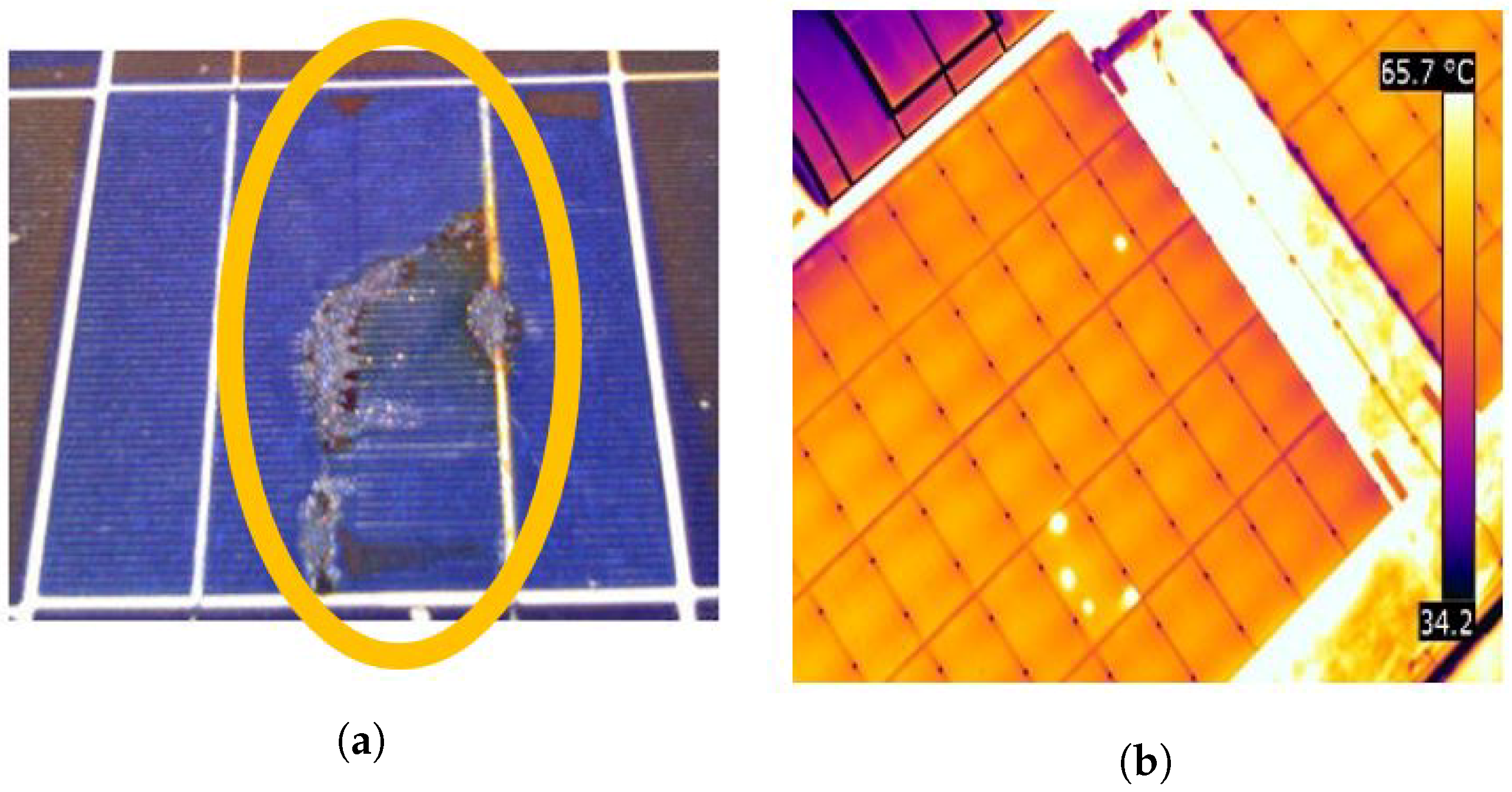
In the conventional process, the hotspot can be found using infrared thermography, where infrared sensors are used to obtain thermal images or thermograms of objects under inspection [33]. The image shows the presence of hotspots as a white spot on the PV panel’s surface. Figure 2a presents an example of cell damage related to the hotspot, and Figure 2b shows an image of hot spot cells captured by an infrared camera [34].
Although the thermography detection method’s performance is effective, the cost of the equipment—especially the infrared camera—is generally quite high, and a workforce for the routine checkup is also needed. Previous studies have presented ideas for hotspot detection in regard to reducing the high maintenance costs. Kim et al. [35] developed AC parameter characterization to represent effects of the hotspot, which are affected by voltage bias, illumination, and temperature. The paper demonstrates the small signal model, which detects the hotspot using the frequency measurement. Kazutaka et al. [36] later presented a simpler model of the hotspot as one of low resistance installed in a circuit equivalent to a single diode. This resistance induces the PV’s current to flow back to the PV cell, and causes a reduction of the output current. Research in Reference [37] presents the simple linear iterative clustering (SLIC) super-pixel technique as the technique for hotspot detection. The topology is to decompose a PV’s thermal image into small homogeneous regions before applying the SLIC to determine the defected cells. The experimental results confirm its efficiency; however, several parameters need to be assigned. Another method is presented in Reference [38] using the door connection method, which utilises a new PV cell connection pattern that can detect the hotspot. Therefore, from the reviews, it is essential to design hotspot detection with high efficiency and simple implementation.
This research paper explains the method of global maximum power point tracking for a PV system under the shading condition, as proposed by the author’s published work [3,39]. The concept behind this algorithm is mountain climbing, where local and global power peaks can be detected without scanning through all of the curves. The algorithm uses information from the trend of the slope from the P–V curve for tracking the accurate PV’s maximum power. Further, this paper proposes the hotspot detection algorithm starting from the hotspot modeling in the scale of the PV’s cell and panel. In relation to the global MPPT algorithm, the hotspot can also be detected based on the trend of the P–V curve. In conclusion, this paper contributes to the advantages of hotspot detection from the implementation towards the efficiency of the results. The proposed method does not require either the infrared or the thermography camera for detecting the fault. Further, the temperature measuring device is not necessary. In terms of the implementation, the system uses simple sensor installation (which requires only one voltage and current sensor set), and simple switching control with the centralized converter.
The usefulness of this research is that the proposed algorithm can be integrated to detect the hotspot within a short period, building the advantage for the PV’s maintenance. According to the literature review, it is critically important to find the hotspot as soon as the fault happens, since the hotspot can spread throughout the whole PV panel. In this way, not only is the power generation reduced, but the severity of the stored heat could also lead to a dangerous fire hazard. The results of the hotspot detection algorithm are presented in the form of graphics with the indicator signal. This signal shows the presence of the hotspot when the algorithm detects the fault. The proposed algorithm is described using the mathematical equations, accompanied by the flowchart and case studies for better understanding.
2. Modeling of PV Panel in Normal and Hotspot Conditions
2.1. Modeling of PV Panel in Normal Condition
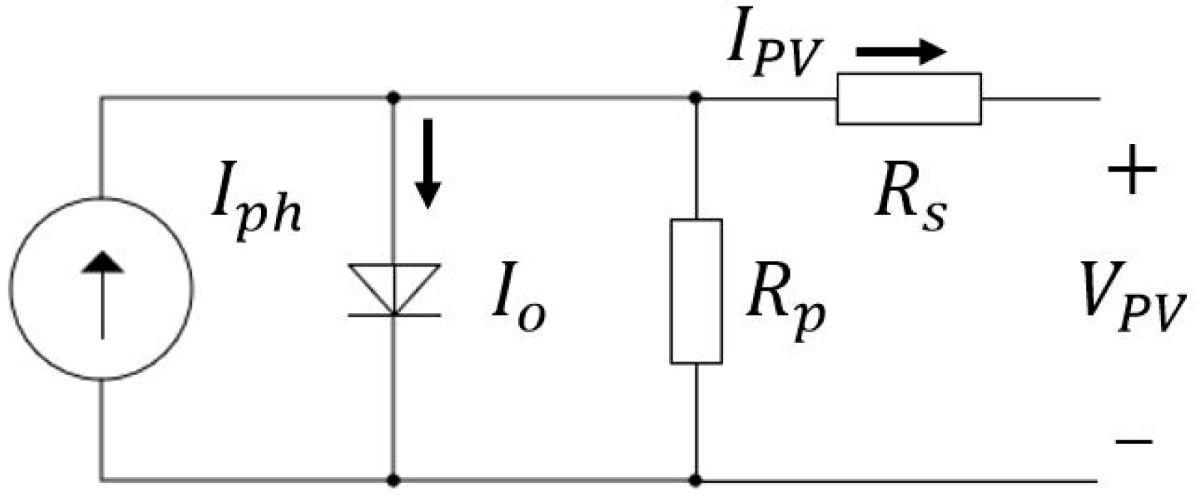
To understand more about the operation of the PV system, the PV’s module can be modeled using the single-diode equivalent circuit [40]. Figure 3 shows the single-diode equivalent circuit including a current source connected in anti-parallel with a diode, including a series resistor and parallel resistor . Equation (1) shows the mathematical relationship between the PV module’s current and other related parameters [41]. Further, Equation (2) presents the expression of the PV module’s open-circuit voltage [42].
From Equation (1), is the PV’s current of the module in the standard test condition (STC), is the temperature coefficient of the current, G is the solar irradiation measured in W/m2, and is the solar irradiation at STC (1000 W/m2). It observes the directly proportional relationship between G and , and when the irradiation increases, the more PV’s current can be obtained. On the other hand, when the irradiation decreases due to shading, the current reduces.
For designing the effective MPPT algorithm, it is necessary to study the operation of PV from the P–V characteristic curves. The work developed by the author in [39] shows the simulation results of P–V curves of 20 different PV panels operated in various irradiation and temperature conditions. The results obtained from the samples show that although the P–V curve has more than one maximum power point, each power peak includes local and global maximum points existing at multiples of 70% to 85% of the PV’s module open-circuit voltage, except for two rightmost sections of the curve in which the peak exists between 75% and 95%. Although the existence of a global power peak varies in each pattern, the peaks are still located within the region. Consequently, the scanning area can be limited. This study is used for designing the global MPP tracking algorithm (the full explanation is shown in Section 3.2).
2.2. Modeling of PV Panel in Hotspot Condition
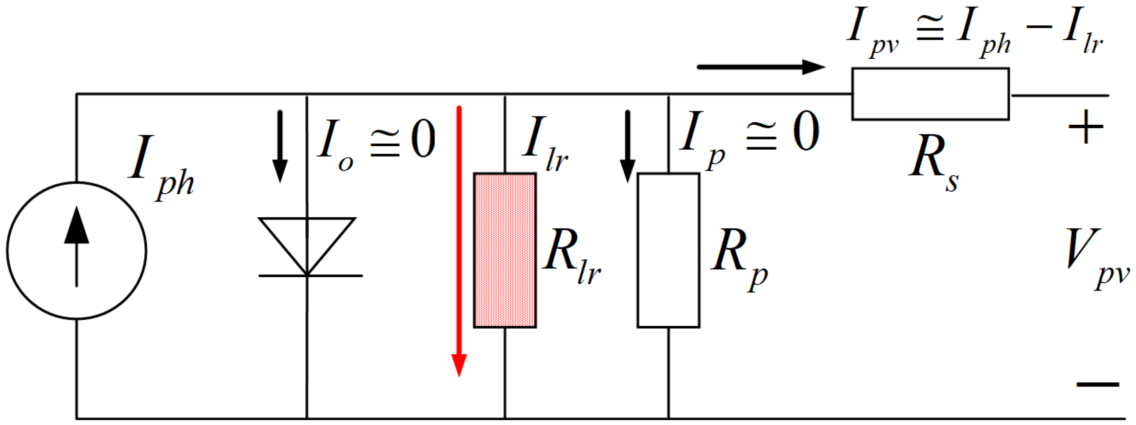
To analyze the behavior of the hotspot, several electrical models have been proposed, as reviewed in the introduction—the interest and simple hotspot modeling circuit by Kazutaka et al. [36]. The proposed work shows the model as the small resistance installed in a PV’s single-diode equivalent circuit. Figure 4 presents the simplified circuit model of a hotspot defected cell.
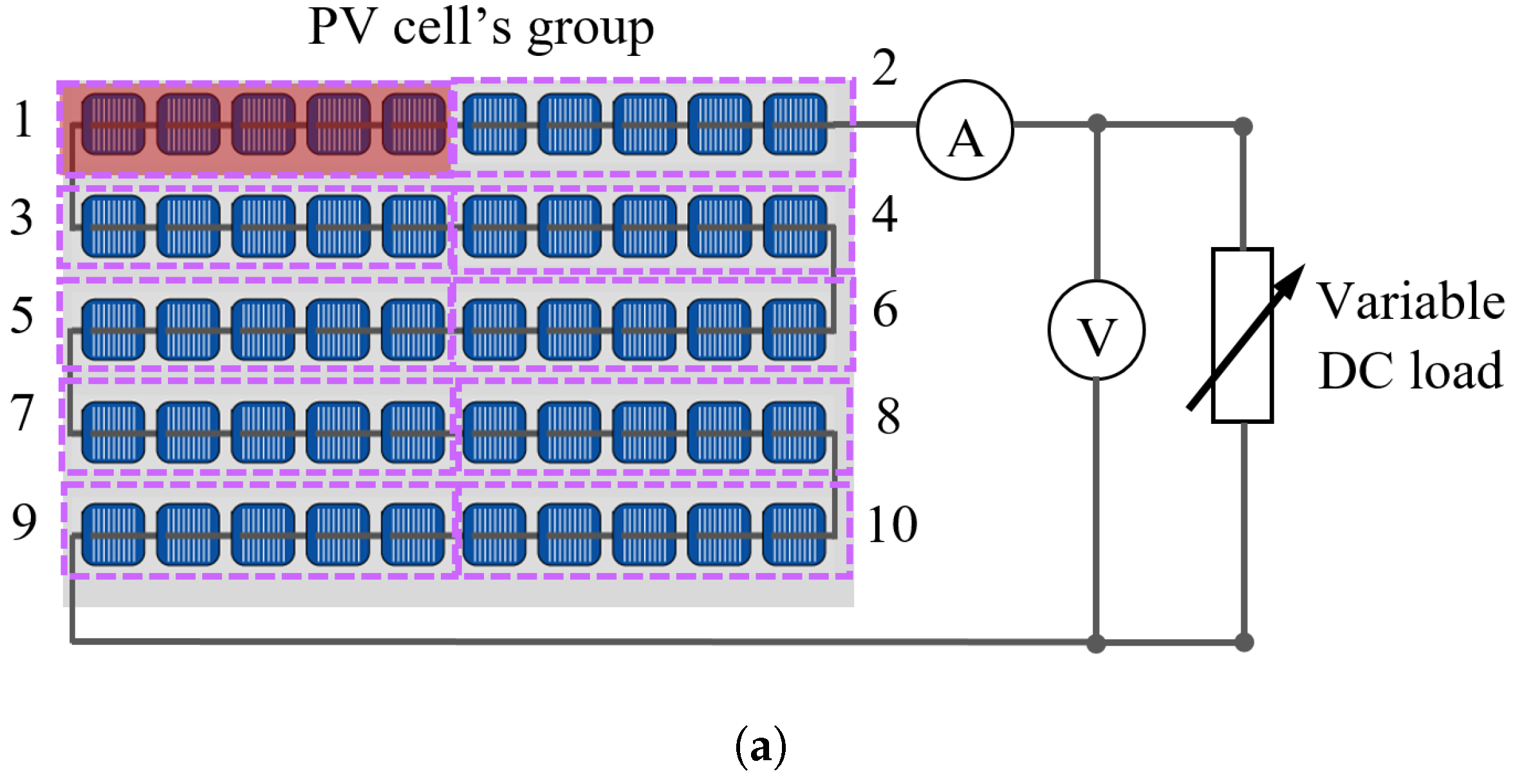
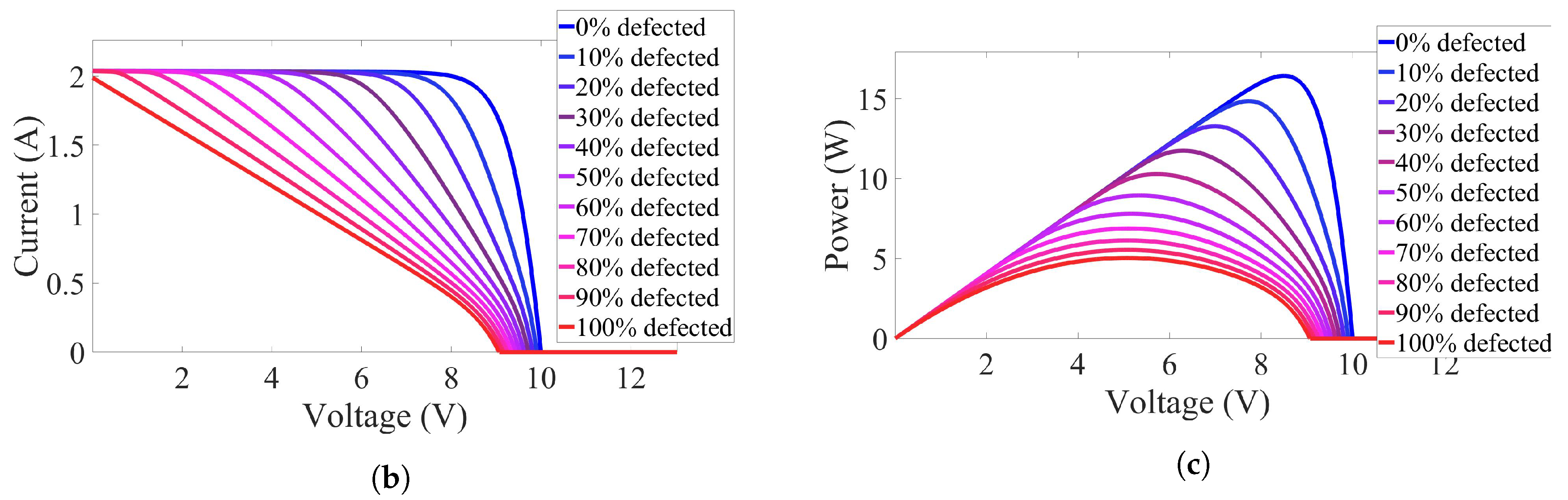
In the modeled circuit, the small resistor represents the defected PV cell. When PV is in operation, this resistance induces the large current which reduces the PV’s output current . This induced current exists inside the module and produces the high level of power dissipation in the PV’s cell. In consequence, the defected PV cell is heated up due to the increase in temperature. Further, if this heat is kept for some time without detection, damage can occur in the form of a hotspot. Although the researchers understand the cause of hotspots, the observation of hotspot occurrence over time is difficult, since the circuit inside the PV cell is not accessible. Direct measurement of the module short-circuit current will not work, since the bypass diode will conduct the current around the defected cell [43]. In this case, another indirect measurement is performed using the I–V and P–V characteristic curve. The proposed approach is similar to the method utilized to determine the cell shunt characteristics by observing the curves under different levels of hotspot-spreading areas. From this data, the worst-case hotspot conditions can be monitored. Information from Reference [44] describes the PV module structure, which consists of many interconnected PV cells connected in series encapsulated into a single stable unit. The model of the PV module is then generated. Figure 5a shows the graphical picture for the PV module with different levels of hotspots from 0% to 100% with an increment of 10% by dividing the PV’s cell into ten groups, and Figure 5b,c displays the I–V and P–V curves from the hotspot levels.
From the results, it can be observed from the I–V curves in Figure 5b that the rate of decrease for the PV’s current varies when the hotspot occurs. Especially in the high percentage of the hotspot, the current drops at a lower PV voltage when compared to the non-defected cells. The occurrence happens from the existence of , which reduces the current to cause them to flow out of the PV cells. Furthermore, the decrease of the current consequently reduces the amount of power generated from the panel, as shown in the P–V curve in Figure 5c. The result from the I–V and P–V curves describes the operation of PV cells when the hotspot happens.
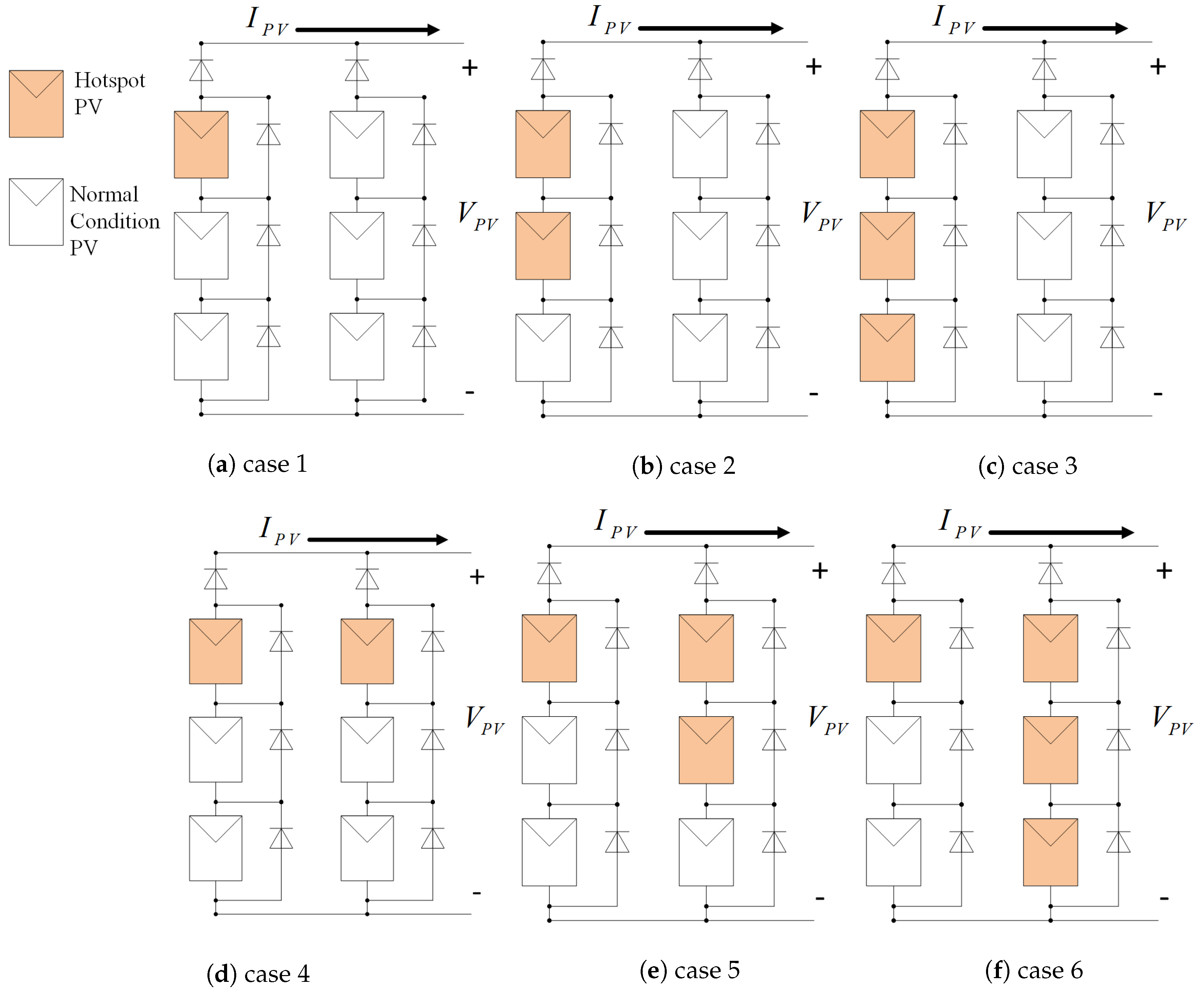
In order to study the effect of the hotspot in the different configuration of the PV array, a simulation was also performed. The configuration shows the series-parallel-connected PV array (two strings in parallel, with three modules for each). Consequently, the connected PV array test was divided into two conditions—series-connected and parallel-connected. The faults in each condition were carried in different positions of the array. Figure 6a–c shows a diagram for the series-connected hotspot (case 1–3) and Figure 6d–f shows the parallel-connected hotspot in the PV array (case 4–6). The PV module that contains the hotspot fault is highlighted in red, while the normal condition panel is not highlighted.
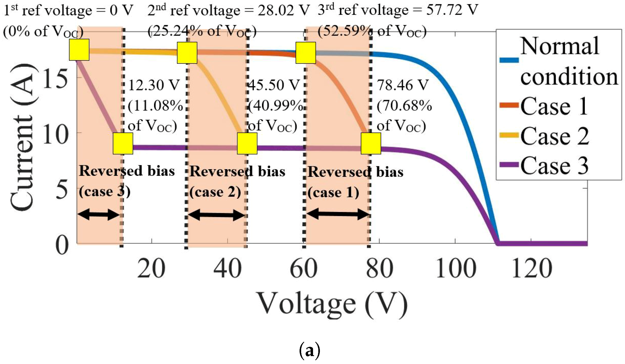
Figure 7a,b displays the I–V curves for all mentioned cases (series-connected hotspot PV array is shown in Figure 7a and parallel-connected hotspot PV array is shown in Figure 7b).
According to the analysis in Figure 4a, the small resistor represents the defected PV cell. When PV is in operation, this resistance induces the large current , which reduces PV’s output current . As shown in Figure 7a, a linear drop in the I–V curves’ region can be observed. This region is called the reverse bias from the hotspot which induces the PV cell to generate less than the normal condition. From the simulation result, the reverse bias region for each case varies from the number of the hotspot in the array. Case 1 contains the hotspot range at 52.59–78.46%, followed by case 2 at 25.24–40.99% and case 3 at 0–11.08%, respectively. As explained in Figure 5b, the more defected cells in the PV system, the less voltage is required for the cell to operate in reverse bias. The reverse bias region in Figure 7a shifts from the right to the left side of the curve, according to the number of defected panels. Moreover, for the simulations for the parallel-connected PV array in Figure 7b, the same trend of reverse bias regions as the series-connected module can be observed. The region is located within the range of 52.59–78.46%, 25.24–40.99%, and 0–11.08%. Furthermore, the PV’s open-circuit voltage observed from the I–V curve decreases to approximately 70% of the normal condition due to the parallel hotspot configuration which reduces the amount voltage. From this initial result, other simulations for larger PV array dimension are also performed to identify the hotspot region.
It is shown that as the number of series-connected panel increases, the more the reverse bias region is divided in the I–V curve. Although the position of the reverse bias region varies from the different specification, their trends can be observed. The hotspot occurrence can be detected by detecting this reverse bias region, using the linear decrease of . Using the greatest divided percentage at 0%, 25%, and 50% of the total , the range for detecting the hotspot can be limited. In using this analysis, the information from the simulation can help authors to design the hotspot-detecting algorithm.
3. Proposed Global MPPT and Hotspot Detection Algorithms
3.1. System Description
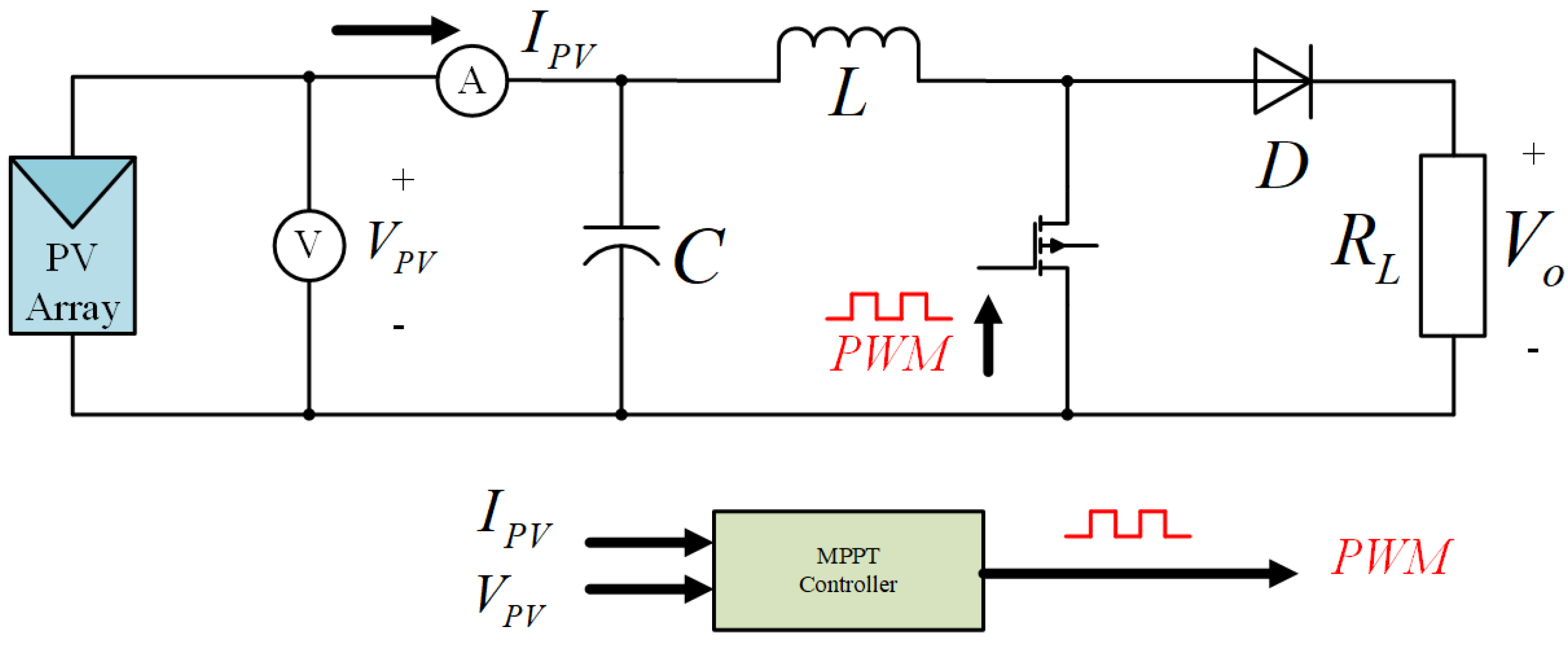
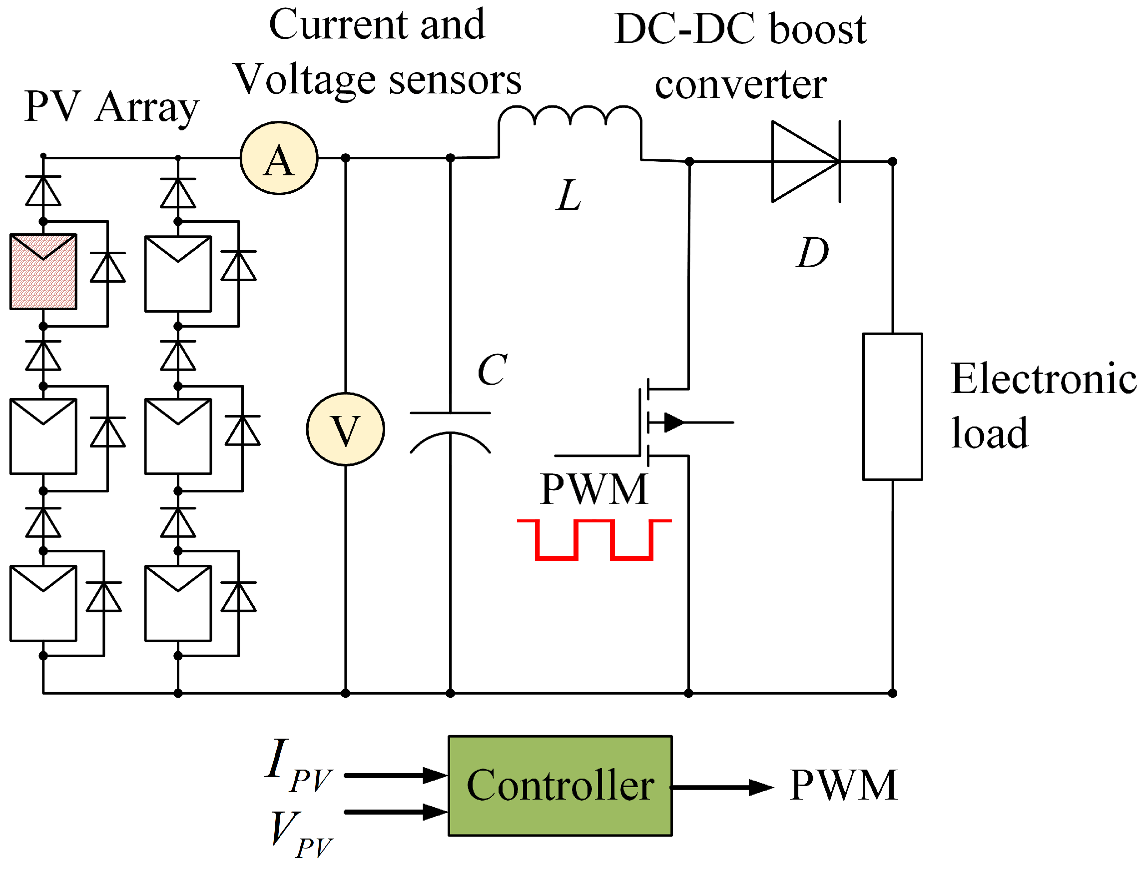
In general, the DC–DC converter for the PV system is used in conjunction with the MPPT controller to control the input voltage and current from the PV to reach its maximum power point. Figure 8 shows the basic PV system block diagram built into the boost converter [44].
Apart from the converter’s circuit, the tested system mainly consists of the voltage and current sensors and the MPPT controller. The MPPT controller determines the maximum power point according to the irradiation level and temperature after measuring the voltage and current of the PV. The controller generates the pulse width modulation (PWM) switching signal to control the PV system to operate at its maximum power. Equation (3) demonstrates the mathematical relations between PV’s voltage , load voltage , and duty cycle d. The challenge to this model is precision. To achieve the accurate at the maximum power, a tracking system is necessary.
In this paper, the DC–DC boost converter was selected to test the proposed global MPPT and hotspot detection algorithms with only one duty cycle value (d) due to its robustness and simple switch control.
3.2. Proposed Global MPPT Algorithm
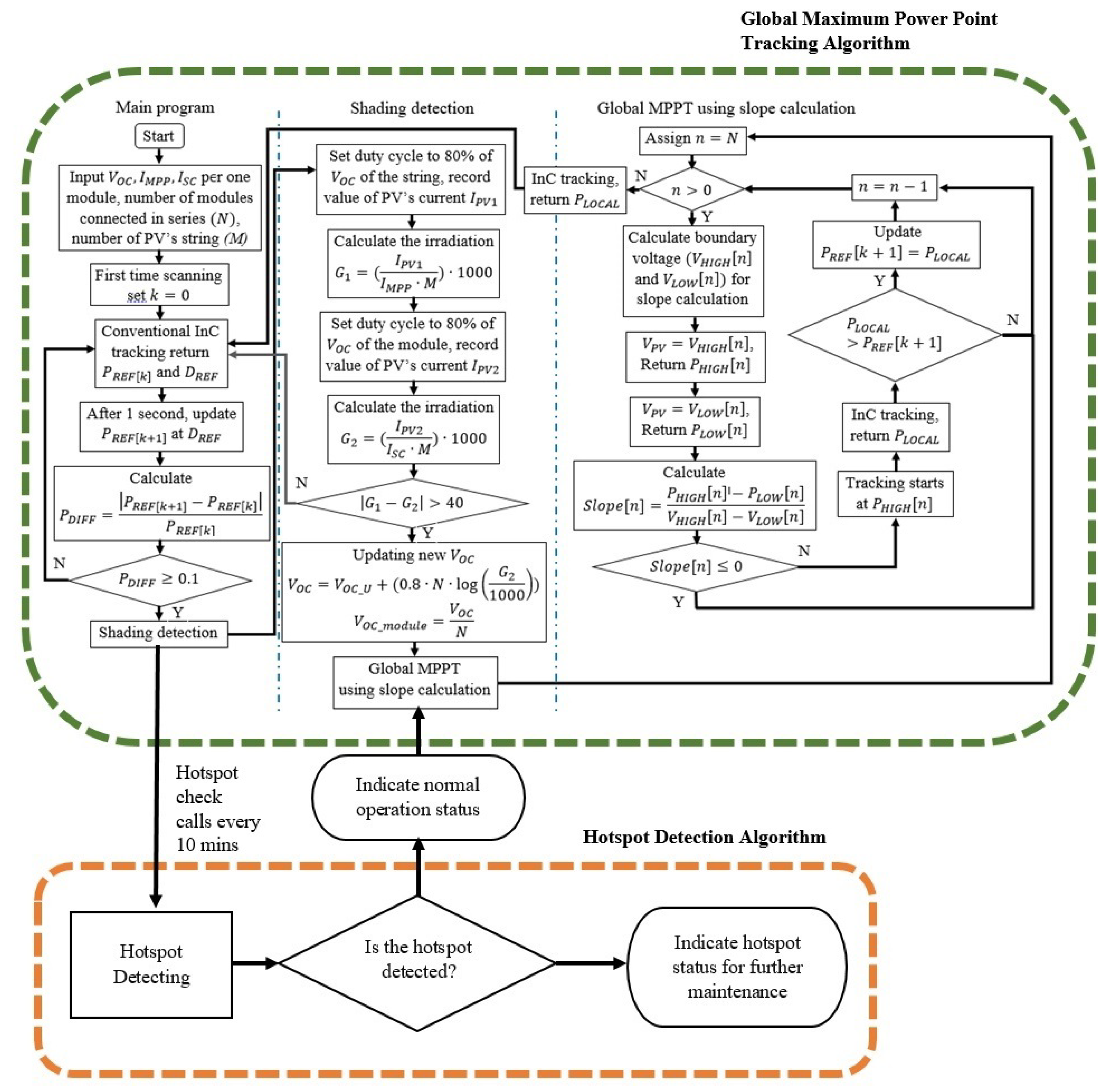
Figure 9 illustrates how the MPPT global algorithm works. It divides mainly into three parts, including the main program, shading detection, and global MPPT tracking using slope calculation.
3.2.1. Main Program
The main part of the algorithm starts from the measurement of PV’s voltage and current also inputting the PV’s module standard parameters, including the single PV module’s open-circuit voltage (), short-circuit current (), and PV’s current at the maximum power point (). Furthermore, the number of modules connected in series (N) and the number of PV’s strings (M) were also inputted. When the program started operating, it was first scanned to determine the first maximum power point. The first tracked power assigned as was located at the duty cycle , and after one second, the next sample of power was updated as . In order to detect the change of power after updating , the ratio of power changes () is calculated. Equation (4) shows how is calculated.
To determine whether the value of is suitable for global MPPT tracking, an appropriate threshold must be selected. If the threshold is too large, MPPT cannot initiate global MPPT, but if it is too small, the algorithm can trigger the wrong trigger with unnecessary global MPPT, causing time and power to be wasted [45]. In order to identify the changes of power for starting global MPPT tracking, the threshold needs to be chosen. Yi-Hwa [46] says that if the threshold is too significant (stated as 15% in the paper), this condition does not guarantee the detection for all shading cases. Moreover, if the threshold is set up to 5%, there is no evidence of the effectiveness of this value, but in practice it is considered too small. Referring to Reference [46] and Seyedmahnoudian in Reference [47], the studies use the threshold of 0.1 (10%) for setting up and usage when the average change of weather condition is assigned. In this case, as the authors’ institution is located in Tokyo, Japan, the weather is generally stable and not rapidly changing. According to the reviews and real meteorological data measured in Tokyo, the threshold of 0.1 is used in this manuscript. If the calculated exceeds the threshold, the program enters the next function—that is, the shading detection—or the program resumes standard InC tracking if the change does not exceed the threshold.
3.2.2. Shading Detection
The next section is shading detection, and the primary purpose of this section is to determine whether or not the changes are due to partial shading. The irradiation is the critical parameter for determining the power changes. For this paper, the simple irradiation estimation is derived from Equation (1) in which the increase of PV’s current is the consequence of the irradiation. This technique is easy to implement. Further, the temperature or irradiation sensors are not required, compared to previous studies. Starting with the calculation, the program calculates irradiation at the short-circuit current of PV and at 80% of the open-circuit voltage of PV’s string. Using the ratio between the measured PV current with and , respectively, and multiplying by 1000, which is the irradiation at STC, and can be achieved. After calculating the irradiations, the difference is compared with the threshold for the shading detection. According to Reference [46], the experiment is performed by testing samples of crystalline PV panels and determining the threshold of difference between the irradiation. The testing achieved the threshold of 40 and this information is applied as the shading detection threshold of the proposed method. If the threshold difference is greater than 40, it means partial shading can occur, and more than one local power peak can exist. After that, the proposed global MPPT algorithm uses slope calculation calls to track the correct MPPT.
From Equation (5), if the absolute difference between and is greater than 40, partial shading has a high chance of occurring. In this case, the value of PV’s open-circuit voltage is updated due to the change in temperature. In this case, the updated can be calculated using Equations (6) and (7). The PV’s open-circuit voltage per one module can also be estimated by dividing with the input number of PV modules, N. is the PV’s open-circuit voltage at STC, and values of PV’s open-circuit voltage can be updated. The new value of contributes more precise and accurate tracking for the proposed algorithm, and short-term testing described in Reference [3] confirms the accuracy.
3.2.3. Global MPPT Using Slope Calculation
The last section of the proposed algorithm is called “Global MPPT using the slope calculation”, which was published in the authors’ published paper [3,39]. The concept of this algorithm is based on the inclined and decreased paths of each section of the P–V curve, which is divided into sections based on the value of the . As stated from the studies of the P–V curves’ patterns in Section 2.1, the location of each power peak exists at multiples of 70% to 85% of the PV’s module open-circuit voltage, except for the two rightmost sections of the curve in which the peak exists between 75% and 95%. The equations are derived based on this study, and the slope calculation chooses from the multiples of each open-circuit voltage in the region deducted by the scaling ratio. Equations (8) and (9) shows the calculation for each slope calculation point on the P–V curve.
N is the number of PV’s module connected in series, and n is the variable assigned in the flowchart in Figure 9. Using Equations (8) and (9), all slope calculation points can be calculated. After the references are recorded, the algorithm starts to calculate the slopes. Equation (10) presents the slope calculation in each region of the P–V curve.
If the calculated slope shows a negative result, it means there is an inclining trend in the region and a power peak can exist. The system then continues tracking for the peak in the region. On the other hand, if the result shows a positive value, it contributes to the declining trend. The system then neglects the tracking and continues to the next region. This method reduces the time required for tracking due to a fewer number of samples needed, compared to the conventional tracking method.
3.3. Proposed Hotspot Detection Algorithm
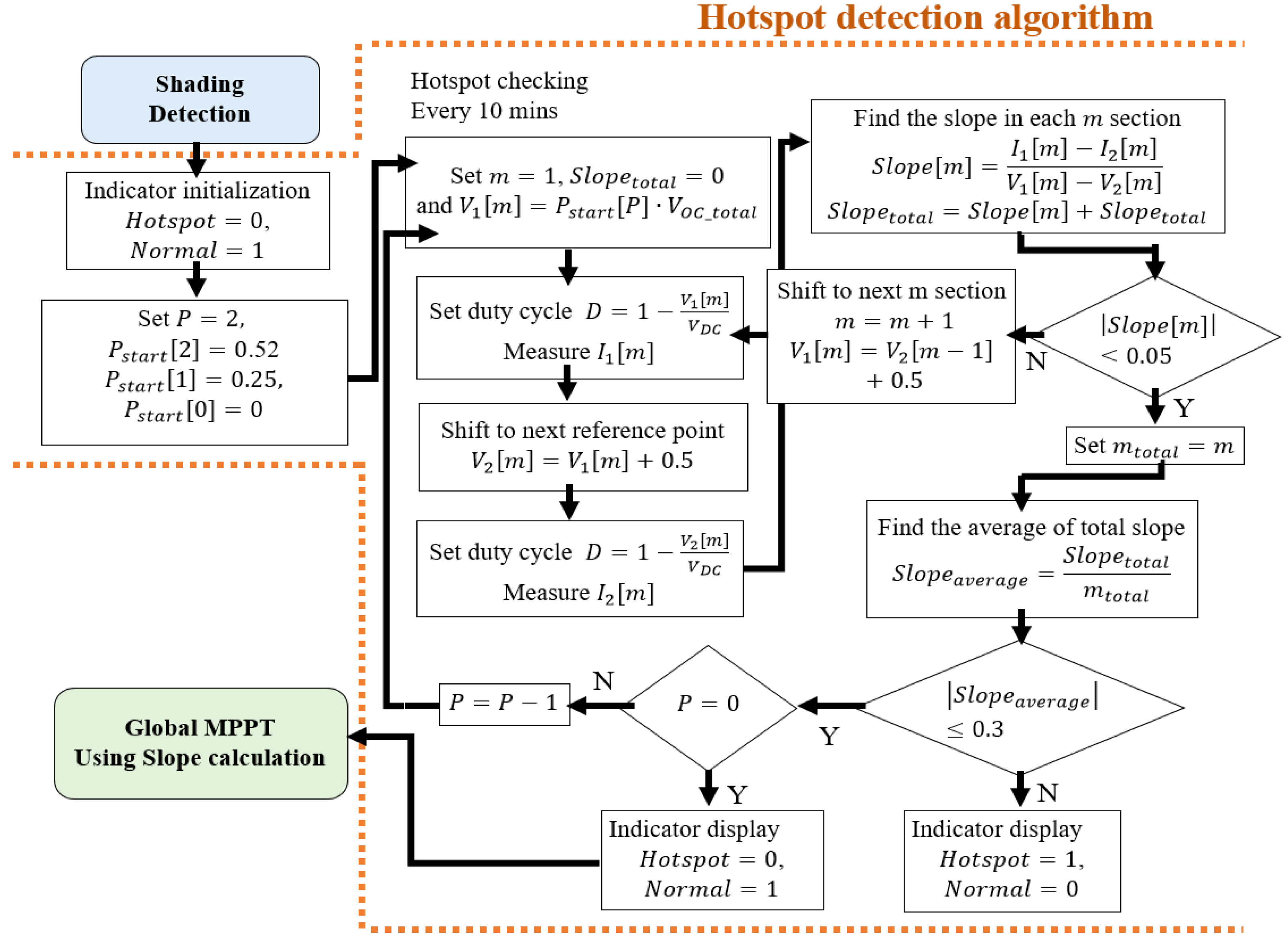
The flowchart in Figure 10 shows how the proposed hotspot detection algorithm operates. As stated in the main flowchart in Figure 9, the hotspot detection algorithm is called every 10 min to check the existence of the hotspot.
From the flowchart, the program calls from the shading detection every 10 min. In particular, the detection shares the input parameters from the Global MPPT algorithm. These include the single PV’s module open-circuit voltage , the number of modules connected in series , and the DC bus voltage . The indicator of fault ( and ) are also introduced. The assigned variable P and navigates the starting point for the three reference regions (at 0%, 25%, and 52%, respectively). When P is 2, the checking starts at the first reference voltage located at 52% of the total , at the point where the value of is recorded and assigned as . The next step repeats after shifting the voltage by 0.5 V to the following reference voltage , and the current is recorded. When two coordinates are filed, the slope for each section can be calculated according to Equation (11).
Using Equation (11), the linear slope of each section was calculated. The value of was used to determine whether the I–V curve shows either the hotspot or normal condition. As the analyses from Figure 6 and Figure 7 show, the reverse bias can be presented when the slope is detected. The threshold checking for each calculated slope was set to be 0.05, and if the value was less than the threshold, it meant the hotspot was not detected, or that it converged to the forward bias region. On the other hand, if the slope was greater than the threshold, it meant the operationwasis still in the reversed bias region, and the algorithm continued to shift to the next reference voltage by 0.5 V.
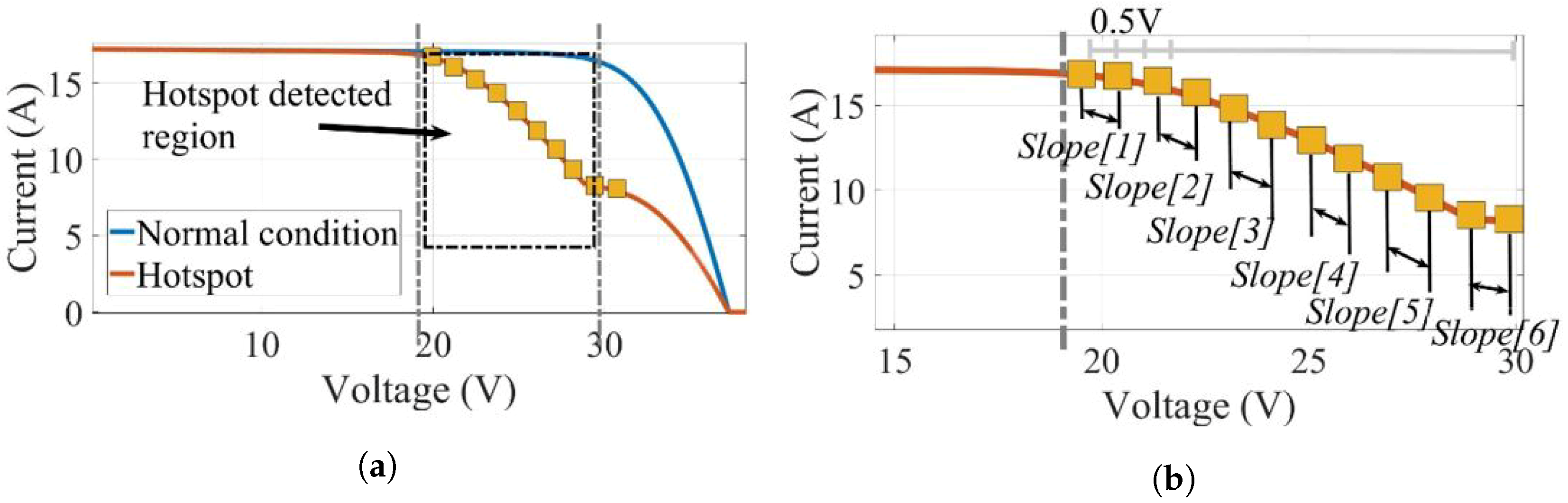
Figure 11a demonstrates how the slope of each section is calculated, and the magnified result is presented in Figure 11b.
Figure 11b demonstrates six sections of slope calculated in the I–V curve. The value of to was computed, and the average value was determined according to the flowchart in Figure 10. The second threshold 0.3 was determined from the test with more than 20 samples of PV modules. If the value of the average slope was greater than the threshold, the hotspot was detected and represented using the indicator. On the other hand, if is less than the threshold, that which defines the hotspot is not found, and the system repeats the process with the next searching region at 25% (P = 1) and 0% (P = 0). When all the regions are checked, and the hotspot is not detected, the system resumes back to the main tracking program.
4. System Implementations and Results
4.1. Simulation Results of the Proposed Global MPPT Algorithm
Dynamic short-term testing in Figure 12a was simulated using MATLAB/Simulink based on the P–V curve shown in Figure 12b.
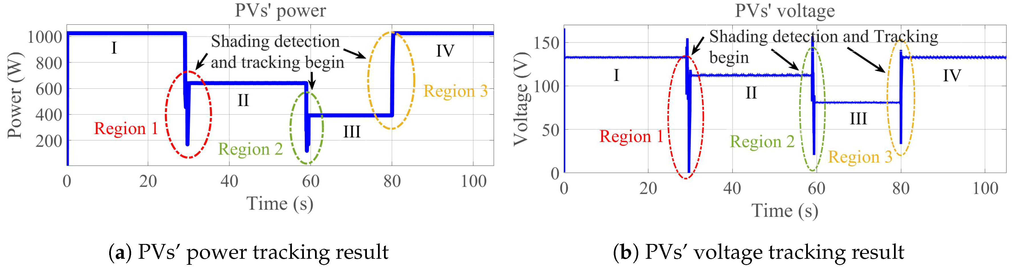
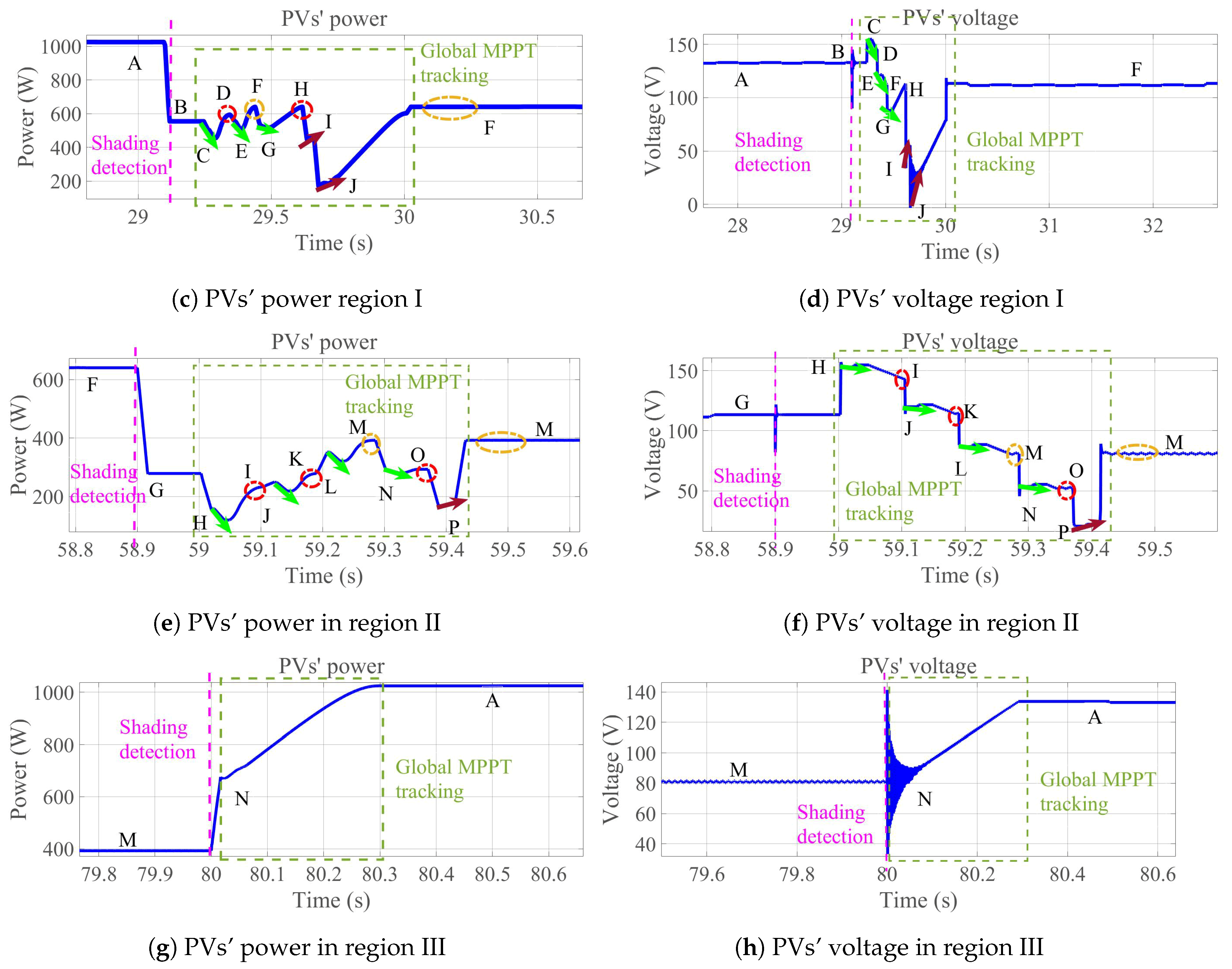
Figure 13a,b shows the complete results of the proposed method, including the tracked power and located voltage. The tracking is divided into three regions, whereas Figure 13c,h magnifies the graphical results in each region for better understanding. Figure 13c shows the magnified global MPPT tracking process in the transition from case I to II. It is observed that the PVs’ power drops from 1023.5 W (point A) to 554.4 W (point B); then the global MPPT starts tracking from point B onwards. Starting from the first slope calculation point of the P–V curve (point C), the tracked slope shows the negative result (represented by the green arrow); the system records the peak value at point D. After that, the algorithm continues the same calculation in other regions by shifting to the next searching region, as the voltage’s transition shows in Figure 13d. All tracked powers are marked at points D, F, and H. For the next region, since the slope of the voltage shows the positive result (represented by the red arrow), the points I and J are then rejected from the power tracking. Finally, the system compares and returns the maximum value, which is point F, as illustrated in Figure 13c. The tracking response time from case I to II takes approximately 0.77 s (0.90 s if the detection time is included).
The slope calculation repeats at the transition of case II to case III, and starts from point G to P in Figure 13e. The change of power decreases from 637.4 W (point F) to 515.2 W (point G) from Figure 13f and most of the searched regions of case III shows the negative slope local power peaks at point I, K, M, and O. All points were compared for the maximum power, and the system returned point M (397.3 W) and stayed stable. The tracking and detection time consumes approximately 0.51 s. Moreover, when the cloud moves away, given the uniform irradiation, the proposed system can also track back from case III onto 1023.5 W (case I) once again. Using 0.27 s for operating, Figure 13g,h demonstrates successful results. To conclude the dynamic testing, it is observed that there was accurate tracking with an excellent transient response, with a fast rising and settling time of approximately 0.51 s on average.
This confirms that the proposed tracking algorithm can operate with high efficiency and accuracy, both in simulation and practical experiments. As presented in the author’s published work [3,39], this algorithm was tested with ten different P–V curves. Both graphical and numerical results prove the effectiveness with tracking time within 3.40 s and the accuracy of 98.62%. Moreover, the system was also simulated in long-term with real weather data measured for 10 h. The test was divided into steady and rapid change based on the weather condition, and the result shows 8.55% total energy enhancement when compared with the conventional method. To sum up, the increase in tracking speed shows in the short-term test that each track has lower power loss than in conventional scanning. Consequently, when operating in the long-term, it increases the energy generated from the PV system. The proposed method can also increase the revenue benefits in the operating day.
4.2. Simulation Results of the Proposed Hotspot Detection Algorithm
The hotspot detection simulation is performed to test the performance of the proposed algorithm. Figure 14 shows the circuit diagram for small-scale testing with the fault highlighted.
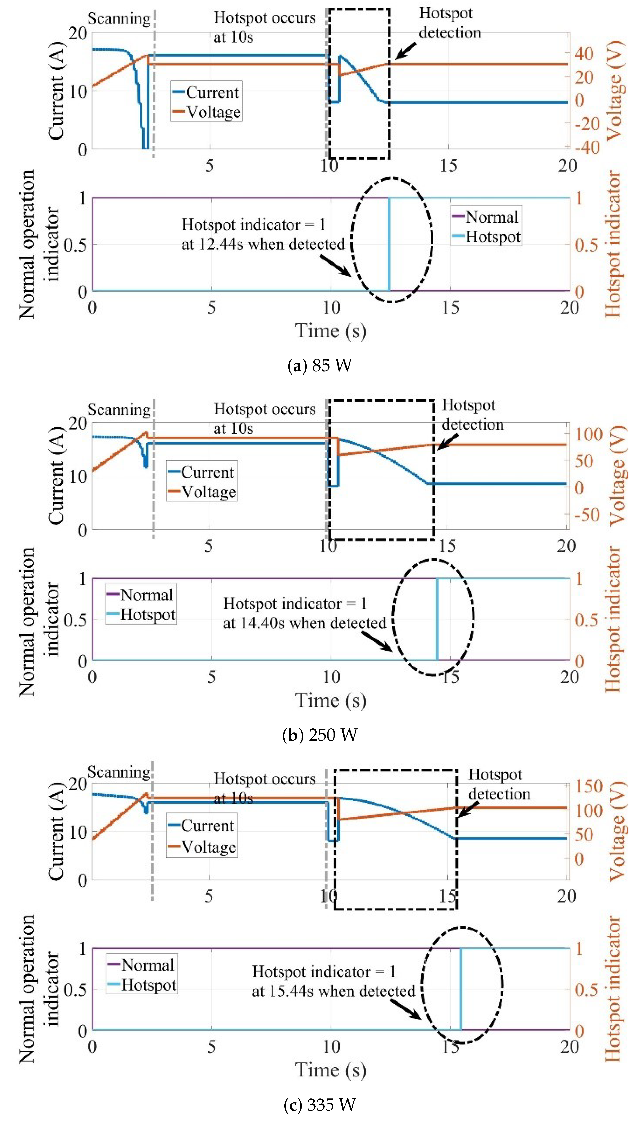
The circuit consists of PV arrays with voltage and current sensors, and a DC–DC boost converter circuit. In order to test the proposed hotspot detection algorithm, the PV array in different configurations was chosen by dividing it into two parts, the small scale (3 × 2) and medium scale (5 × 5). The simulation was performed using three PV specifications stated in the introduction. Figure 15 demonstrates the graphical result from Simulink for the circuit in Figure 14 in different PV specifications. The Figure includes (1) DMSolar 85 W from DMSolar LLC; Florida USA for Figure 15a, (2) 1Soltech 250 W from 1Soltech Inc; Texas USA for Figure 15b, and (3) American Choice Solar 335 W from American Choice Energy LLC; Florida USA for Figure 15c.
According to the graphical results, the hotspot was set to happen at 10 s based on the simulation time. The result confirms the principle of the proposed hotspot detection algorithm. For the 85W PV module in Figure 15a, it started from scanning to find the maximum power from 0 to 2.35 s, and the system operated at constant PV power before the hotspot happened. After 10 s, the hotspot occurred and the proposed detection program started to operate. The detection started from the first reference point and continued until the fault was detected. At 12.44 s, the hotspot was found by the system and the indicator changed the status from to . Figure 15b,c also confirms the operation of the proposed hotspot detection system. Using the same principle mentioned in Figure 15a, the hotspot was successfully found at 14.40 s for 250 W PV module and 15.44 s for the 335 W PV module. Table 1 summarizes the numerical result, including the and the tracking time for each PV specification. The algorithm took a maximum tracking time of 5.44 s. Both graphical and numerical results confirm the success of the proposed hotspot detection algorithm.
For the small-scale simulation, both graphical and numerical results confirm the effectiveness of the proposed hotspot detection method. Although the PV specifications are different, the reversed bias region presented in each I–V curve represents the hotspot, and the program operated successfully. Consequently, the different PV specifications and the hotspot also varied in several locations in the PV array. The medium-scale simulation demonstrates the ability of the operation to detect the hotspot in larger-scale arrays and various hotspot locations.
4.3. Simulation Results—Medium Scale
The proposed hotspot-detecting algorithm was tested with 5 × 5 PV arrays, using a DMSolar 85 W panel. It consisted of four cases from A to D, and the position of the hotspot varied in several PV panels. The location of the fault was represented using different highlighted colors, shown in Figure 16.
Figure 17 demonstrates the graphical results for each case. The proposed algorithm starts its operation by scanning for the first maximum power, taking approximately 2.30 s of the simulation time. After the hotspot occurs at 10.00 s, the program starts to identify the changes in PV’s power and continues detecting the hotspot. If the hotspot is found, the indicator shows the fault status changing from to after the detection succeeds. For the numerical results, Table 2 summarizes the information, including the and the tracking time for each hotspot case.
Overall, both graphical and numerical results confirm the success of the proposed hotspot detection method. Although the hotspots’ location varied in the PV array, the program was capable to detect the fault presented by the indicator. Using the information from Section 2.2 on hotspot-modeling, the program was designed and proven from the small- and medium-scale testing. The algorithm also provides accurate results with fast detection time.
5. Conclusions
This paper presented two algorithms that can enhance the performance of the PV system, including the global MPPT under the shading condition and the hotspot detection algorithm. The proposed global MPPT algorithm is derived based on the trend of PV’s characteristic curves, dividing the curves into searching regions and tracking from the slope of each section. In addition, the proposed hotspot detection algorithm is also implemented. This algorithm integrates with the global MPPT and indicates when the hotspot occurs in the PV system. The global MPPT shows the efficiency with tracking time within 0.51 s and accuracy to detect the power in the dynamic test with fast rising and settling time. The hotspot detection demonstrates the accuracy when testing with different hotspot locations in various PV configurations. Results were presented in graphical and numerical formto confirm the effectiveness of the proposed algorithm, with a maximum tracking time of 5.44 s.
Author Contributions
J.G. conceived the methodology, developed the theory, performed the computations and prepared this paper. G.F. performed the supervision, provided critical feedback and helped shaping the research.
Funding
This research received no external funding.
Acknowledgments
The authors would like to tribute the acknowledgment towards the colleagues in power system laboratory, Shibaura Institute of Technology for all information and technical support.
Conflicts of Interest
The authors declare no conflict of interest.
Abbreviations
The following abbreviations are used in this manuscript:
| ANN | Artificial Neural Network |
| d | Duty Cycle |
| DSP | Digital Signal Processor |
| G | Irradiation |
| GMPPT | Global Maximum Power Point Tracking |
| I–V | Current–Voltage |
| InC | Incremental Conductance |
| MDPI | Multidisciplinary Digital Publishing Institute |
| MPP | Maximum Power Point |
| MPPT | Maximum Power Point Tracking |
| P & O | Perturb and Observe |
| P–V | Power–Voltage |
| PSO | Particle Swarm Optimization |
| PV | Photovoltaic |
| PWM | Pulse Width Modulation |
| SLIC | Simple Linear Iterative Clustering |
| STC | Standard Test Condition |
| T | Temperature |
References
- Romero-Cadaval, E.; Spagnuolo, G.; Franquelo, L.G.; Ramos-Paja, A.C.; Suntio, T.; Xiao, W.M. Grid-Connected Photovoltaic Generation Plants: Components and Operation. IEEE Ind. Electron. Mag. 2013, 7, 6–20. [Google Scholar] [CrossRef] [Green Version]
- Patel, H.; Agarwal, V. MATLAB-Based Modeling to Study the Effects of Partial Shading on PV Array Characteristics. IEEE Trans. Energy Convers. 2008, 23, 302–310. [Google Scholar] [CrossRef]
- Gosumbonggot, J.; Fujita, G. Partial Shading Detection and Global Maximum Power Point Tracking Algorithm for Photovoltaic with the Variation of Irradiation and Temperature. Energies 2019, 12, 202. [Google Scholar] [CrossRef]
- Femia, N.; Lisi, G.; Petrone, G.; Spagnuolo, G.; Vitelli, M. Distributed maximum power point tracking of photovoltaic arrays: Novel approach and system analysis. IEEE Trans. Ind. Electron. 2008, 55, 2610–2621. [Google Scholar] [CrossRef] [Green Version]
- Gao, L.; Dougal, R.A.; Liu, S.; Iotova, A.P. Parallel-Connected Solar PV System to Address Partial and Rapidly Fluctuating Shadow Conditions. IEEE Trans. Ind. Electron. 2009, 56, 1548–1556. [Google Scholar] [CrossRef] [Green Version]
- Eftichios, K. A New Technique for Tracking the Global Maximum Power Point of PV Arrays Operating Under Partial-Shading Conditions. IEEE J. Photovolt. 2012, 2, 184–190. [Google Scholar] [CrossRef] [Green Version]
- Daraban, S.; Petreus, D.; Morel, C.; Machmoum, M. A novel global MPPT algorithm for distributed MPPT systems. In Proceedings of the 2013 15th European Conference on Power Electronics and Applications (EPE), Lille, France, 2–6 September 2013; pp. 1–10. [Google Scholar] [CrossRef]
- Pillai, D.S.; Rajasekar, N. A comprehensive review on protection challenges and fault diagnosis in PV systems. Renew. Sustain. Energy Rev. 2018, 91, 18–40. [Google Scholar] [CrossRef]
- Veerachary, M. PSIM circuit-oriented simulator model for the nonlinear photovoltaic sources. IEEE Trans. Aerosp. Electron. Syst. 2006, 42, 735–740. [Google Scholar] [CrossRef]
- Tey, K.S.; Mekhilef, S. Modified Incremental Conductance Algorithm for Photovoltaic System Under Partial Shading Conditions and Load Variation. IEEE Trans. Ind. Electron. 2014, 61, 5384–5392. [Google Scholar] [CrossRef]
- Ji, Y.; Jung, D.; Won, C.; Lee, B.; Kim, J. Maximum power point tracking method for PV array under partially shaded condition. In Proceedings of the 2009 IEEE Energy Conversion Congress and Exposition, San Jose, CA, USA, 20–24 September 2009; pp. 307–312. [Google Scholar] [CrossRef]
- Sera, D.; Mathe, L.; Kerekes, T.; Spataru, S.V.; Teodorescu, R. On the Perturb-and-Observe and Incremental Conductance MPPT Methods for PV Systems. IEEE J. Photovolt. 2013, 3, 1070–1078. [Google Scholar] [CrossRef]
- Nguyen, T.L.; Low, K. A Global Maximum Power Point Tracking Scheme Employing DIRECT Search Algorithm for Photovoltaic Systems. IEEE Trans. Ind. Electron. 2010, 57, 3456–3467. [Google Scholar] [CrossRef]
- Malik, S. MPPT Schemes for PV System under Normal and Partial Shading Condition: A Review. Int. J. Renew. Energy Dev. 2016, 2, 79–94. [Google Scholar]
- Alik, R.; Jusoh, A.; Shukri, N.A. An improved perturb and observe checking algorithm MPPT for photovoltaic system under partial shading condition. In Proceedings of the 2015 IEEE Conference on Energy Conversion (CENCON), Johor Bahru, Malaysia, 19–20 October 2015. [Google Scholar]
- Kapić, A.; Zečević, Ž.; Krstajić, B. An efficient MPPT algorithm for PV modules under partial shading and sudden change in irradiance. In Proceedings of the 2018 23rd International Scientific-Professional Conference on Information Technology (IT), Zabljak, Montenegro, 19–24 February 2018. [Google Scholar] [CrossRef]
- Duan, Q.; Leng, J.; Duan, P.; Hu, B.; Mao, M. An Improved Variable Step PO and Global Scanning MPPT Method for PV Systems under Partial Shading Condition. In Proceedings of the 2015 7th International Conference on Intelligent Human-Machine Systems and Cybernetics, Hangzhou, China, 26–27 August 2015. [Google Scholar] [CrossRef]
- Başoğlu, M.E.; Çakir, B. Experimental evaluations of global maximum power point tracking approaches in partial shading conditions. In Proceedings of the 2017 IEEE International Conference on Environment and Electrical Engineering and 2017 IEEE Industrial and Commercial Power Systems Europe (EEEIC/I&CPS Europe), Milan, Italy, 6–9 June 2017. [Google Scholar] [CrossRef]
- Bidyadhar, S. A Comparative Study on Maximum Power Point Tracking Techniques for Photovoltaic Power Systems. IEEE Trans. Sustain. Energy 2013, 4, 89–97. [Google Scholar] [CrossRef]
- Kinattigal, S. Enhanced Energy Output From a PV System Under Partial Shading Conditions through Artifical Bee Colony. IEEE Trans. Sustain. Energy 2015, 6, 198–209. [Google Scholar] [CrossRef]
- Kobayashi, K.; Takano, I.; Sawada, Y. A study on a two stage maximum power point tracking control of a photovoltaic system under partially shaded insolation conditions. In Proceedings of the 2003 IEEE Power Engineering Society General Meeting (IEEE Cat. No.03CH37491), Toronto, ON, Canada, 13–17 July 2003; pp. 2612–2617. [Google Scholar] [CrossRef]
- Irisawa, K.; Saito, T.; Takano, I.; Sawada, Y. Maximum power point tracking control of photovoltaic generation system under non-uniform insolation by means of monitoring cells. In Proceedings of the Conference Record of the Twenty-Eighth IEEE Photovoltaic Specialists Conference, Anchorage, AK, USA, 15–22 September 2000; pp. 1707–1710. [Google Scholar] [CrossRef]
- Miyatake, M.; Veerachary, M.; Toriumi, F.; Fujii, N.; Ko, H. Maximum Power Point Tracking of Multiple Photovoltaic Arrays: A PSO Approach. IEEE Trans. Aerosp. Electron. Syst. 2011, 367–380. [Google Scholar] [CrossRef]
- Yuan, X.; Yang, D.; Liu, H. MPPT of PV system under partial shading condition based on adaptive inertia weight particle swarm optimization algorithm. In Proceedings of the 2015 IEEE International Conference on Cyber Technology in Automation, Control, and Intelligent Systems (CYBER), Shenyang, China, 8–12 June 2015. [Google Scholar] [CrossRef]
- Ishaque, K.; Salam, Z.; Amjad, M.; Mekhilef, S. An Improved Particle Swarm Optimization (PSO)–Based MPPT for PV with Reduced Steady-State Oscillation. IEEE Trans. Power Electron. 2012, 3627–3638. [Google Scholar] [CrossRef]
- Alajmi, B.N.; Ahmed, K.H.; Finney, S.J.; Williams, B.W. A Maximum Power Point Tracking Technique for Partially Shaded Photovoltaic Systems in Microgrids. IEEE Trans. Ind. Electron. 2013, 1596–1606. [Google Scholar] [CrossRef]
- ABB. Available online: https://library.e.abb.com/public/10bc5e66068c4f768a1d77fd853a7e4e/PVI-3.0-3.6-4.2_BCD.00374_EN_RevG.pdf (accessed on 6 October 2018).
- SMA. Available online: http://files.sma.de/dl/15330/SB5000TL-21-DEN1551-V20web.pdf (accessed on 8 October 2018).
- Lyden, S.; Haque, M.E.; Gargoom, A.; Negnevitsky, M. Review of Maximum Power Point Tracking approaches suitable for PV systems under Partial Shading Conditions. In Proceedings of the 2013 Australasian Universities Power Engineering Conference (AUPEC), Hobart, TAS, Australia, 29 September–3 October 2013; pp. 1–6. [Google Scholar] [CrossRef]
- Tamizh-Mani, M.G. Failure and Degradation Modes of PV Modules in a Hot Dry Climate; NREL: Golden, CO, USA, 2018. Available online: https://www.energy.gov/sites/prod/files/2014/01/f7/pvmrw13_openingsession_asu_mani.pdf (accessed on 4 January 2019).
- Olalla, C.; Hasan, M.; Deline, C.; Maksimović, D. Mitigation of Hot-Spots in Photovoltaic Systems using Distributed Power Electronics. Energies 2018, 11, 726. [Google Scholar] [CrossRef]
- Rossi, D.; Omana, M.; Giaffreda, D.; Metra, C. Modeling and Detection of Hotspot in Shaded Photovoltaic Cells. IEEE Trans. Very Large Scale Integr. (VLSI) Syst. 2015, 23, 1031–1039. [Google Scholar] [CrossRef] [Green Version]
- Salazar, M. Hotspots Detection in Photovoltaic Modules Using Infrared Thermography. In Proceedings of the ICMIT 2016, Bangkok, Thailand, 19–22 September 2016. [Google Scholar]
- Paul Kitawa. Available online: https://www.kitawa.de/en/thermography-pv-systems (accessed on 29 November 2018).
- Kim, K.A.; Seo, B.C.G.; Krein, P.T. Photovoltaic Hot-Spot Detection for Solar Panel Substrings Using AC Parameter Characterization. IEEE Trans. Power Electron. 2016, 31, 1121–1130. [Google Scholar] [CrossRef]
- Yang, S.; Itako, K.; Kudoh, T.; Koh, K.; Ge, Q. Monitoring and Suppression of the Typical Hot-Spot Phenomenon Resulting From Low-Resistance Defects in a PV String. IEEE J. Photovolt. 2018, 8, 1809–1817. [Google Scholar] [CrossRef]
- Alsafasfeh, M.; Abdel-Qader, I.; Bazuin, B. Fault detection in photovoltaic system using SLIC and thermal images. In Proceedings of the 2017 8th International Conference on Information Technology (ICIT), Amman, Jordan, 17–18 May 2017; pp. 672–676. [Google Scholar]
- Dong, F.; Hou, M.; Feng, H.; Jin, Z.; Tian, J. Research on the reconstruction method of PV module based on the door connection. In Proceedings of the 2016 IEEE PES Asia-Pacific Power and Energy Engineering Conference (APPEEC), Xi’an, China, 25–28 October 2016; pp. 337–341. [Google Scholar]
- Gosumbonggot, J. Partial Shading and Global Maximum Power Point Detection Enhancing MPPT for Photovoltaic Systems Operated in Shading Condition. In Proceedings of the 2018 53rd International Universities Power Engineering Conference (UPEC), Glasgow, UK, 4–7 September 2018. [Google Scholar] [CrossRef]
- Karim, D. Backstepping sliding mode control for maximum power point tracking of a photovoltaic system. Electr. Power Syst. Res. 2017, 143, 182–188. [Google Scholar]
- Moballegh, S.; Jiang, J. Modeling, Prediction, and Experimental Validations of Power Peaks of PV Arrays under Partial Shading Conditions. IEEE Trans. Sustain. Energy 2014, 293–300. [Google Scholar] [CrossRef]
- Hiren, P. Maximum Power Point Tracking Scheme for PV Systems Operating Under Partially Shaded Conditions. IEEE Trans. Ind. Electron. 2008, 55, 1689–1698. [Google Scholar] [CrossRef] [Green Version]
- Wohlgemuth, J.; Herrmann, W. Hot spot tests for crystalline silicon modules. In Proceedings of the Conference Record of the Thirty-First IEEE Photovoltaic Specialists Conference, Lake Buena Vista, FL, USA, 3–7 January 2005; pp. 1062–1063. [Google Scholar]
- PVEducation. Available online: https://www.pveducation.org/pvcdrom/modules/modules-structure (accessed on 7 January 2019).
- Ahmed, J. An accurate method for MPPT algorithm to detect the Partial shading Occurrence in a PV system. IEEE Trans. Ind. Inform. 2017, 13. [Google Scholar] [CrossRef]
- Liu, Y.H.; Huang, S.C.; Huang, J.W.; Liang, W.C. A particle swarm optimization-based maximum power point tracking algorithm for PV systems operating under partially shaded conditions. IEEE Trans. Energy Convers. 2012, 27. [Google Scholar] [CrossRef]
- Seyedmahmoudian, M. Simulation and hardware implementation of new maximum power point tracking technique for partially shaded PV system using hybrid DEPSO method. IEEE Trans. Sustain. Energy 2015, 6. [Google Scholar] [CrossRef]
Figure 1.
(a) Standard test condition at 25 C, (b) Partial Shading condition at 25 C, (c) current–voltage (I–V) characteristic curves for both conditions, (d) power–voltage (P–V) characteristic curves for both conditions.
Figure 1.
(a) Standard test condition at 25 C, (b) Partial Shading condition at 25 C, (c) current–voltage (I–V) characteristic curves for both conditions, (d) power–voltage (P–V) characteristic curves for both conditions.

Figure 2.
(a) Cell damage related to a hot spot; (b) an example of hot spot cells captured by an infrared camera.
Figure 2.
(a) Cell damage related to a hot spot; (b) an example of hot spot cells captured by an infrared camera.

Figure 3.
PV’s module equivalent circuit.

Figure 4.
Simplified model of a hotspot defected cell.

Figure 5.
(a) Simulation circuit diagram for different levels of hotspots in a PV panel; (b) I–V characteristic curves for different levels of hotspots; (c) P–V characteristic curves for different levels of hotspots.
Figure 5.
(a) Simulation circuit diagram for different levels of hotspots in a PV panel; (b) I–V characteristic curves for different levels of hotspots; (c) P–V characteristic curves for different levels of hotspots.


Figure 6.
Diagram for the hotspot PV array: (a) case 1; (b) case 2; (c) case 3; (d) case 4; (e) case 5; (f) case 6.
Figure 6.
Diagram for the hotspot PV array: (a) case 1; (b) case 2; (c) case 3; (d) case 4; (e) case 5; (f) case 6.

Figure 7.
I–V characteristic curve for the hotspot PV array: (a) series-connected (case 1–3), and (b) parallel-connected (case 4–6).
Figure 7.
I–V characteristic curve for the hotspot PV array: (a) series-connected (case 1–3), and (b) parallel-connected (case 4–6).


Figure 8.
Basic PV system with DC–DC boost converter.

Figure 9.
Flowchart of proposed Global MPPT algorithm.

Figure 10.
Flowchart of proposed hotspot detection algorithm.

Figure 11.
Example I–V characteristic curve for hotspot detection algorithm: (a) full I–V curve; (b) magnified reverse bias region.
Figure 11.
Example I–V characteristic curve for hotspot detection algorithm: (a) full I–V curve; (b) magnified reverse bias region.

Figure 12.
(a) Dynamic short-term testing diagram; (b) P–V characteristic curves under dynamic change by a passed cloud.
Figure 12.
(a) Dynamic short-term testing diagram; (b) P–V characteristic curves under dynamic change by a passed cloud.

Figure 13.
Results from proposed algorithm: (a) PVs’ Power tracking result; (b) PVs’ Voltage result; (c,e,g) Magnified power tracking result for each region; (d,f,h) Magnified voltage tracking result for each region.
Figure 13.
Results from proposed algorithm: (a) PVs’ Power tracking result; (b) PVs’ Voltage result; (c,e,g) Magnified power tracking result for each region; (d,f,h) Magnified voltage tracking result for each region.


Figure 14.
Simulation circuit diagram for hotspot detection.

Figure 15.
Simulation result for the proposed hotspot detection algorithm using different PV specifications.
Figure 15.
Simulation result for the proposed hotspot detection algorithm using different PV specifications.

Figure 16.
Simulation circuit diagram for hotspot detection.

Figure 17.
Simulation result for the proposed hotspot detection algorithm using a medium-scale PV array: (a) case A; (b) case B; (c) case C; (d) case D.
Figure 17.
Simulation result for the proposed hotspot detection algorithm using a medium-scale PV array: (a) case A; (b) case B; (c) case C; (d) case D.


Table 1.
Numerical result for the proposed hotspot detection algorithm using different PV specifications: (a) 85 W; (b) 250 W; and (c) 335 W.
Table 1.
Numerical result for the proposed hotspot detection algorithm using different PV specifications: (a) 85 W; (b) 250 W; and (c) 335 W.
| PV Specification | Tracking Time (s) | |
|---|---|---|
| DMSolar 85 W | −0.79 | 2.44 |
| 1Soltech 250 W | −0.44 | 4.40 |
| American Choice Solar 335 W | −0.34 | 5.44 |
Table 2.
Numerical result for the proposed hotspot detection algorithm in medium-scale.
| Hotspot Case | Tracking Time (s) | |
|---|---|---|
| Case A | −0.49 | 3.63 |
| Case B | −0.72 | 3.94 |
| Case C | −0.79 | 3.96 |
| Case D | −1.02 | 4.02 |
© 2019 by the authors. Licensee MDPI, Basel, Switzerland. This article is an open access article distributed under the terms and conditions of the Creative Commons Attribution (CC BY) license (http://creativecommons.org/licenses/by/4.0/).
Share and Cite
MDPI and ACS Style
Gosumbonggot, J.; Fujita, G. Global Maximum Power Point Tracking under Shading Condition and Hotspot Detection Algorithms for Photovoltaic Systems. Energies 2019, 12, 882. https://doi.org/10.3390/en12050882
AMA Style
Gosumbonggot J, Fujita G. Global Maximum Power Point Tracking under Shading Condition and Hotspot Detection Algorithms for Photovoltaic Systems. Energies. 2019; 12(5):882. https://doi.org/10.3390/en12050882
Chicago/Turabian StyleGosumbonggot, Jirada, and Goro Fujita. 2019. "Global Maximum Power Point Tracking under Shading Condition and Hotspot Detection Algorithms for Photovoltaic Systems" Energies 12, no. 5: 882. https://doi.org/10.3390/en12050882
Note that from the first issue of 2016, this journal uses article numbers instead of page numbers. See further details here.