Neural Network-Based Model Reference Adaptive System for Torque Ripple Reduction in Sensorless Poly Phase Induction Motor Drive


1
Department of Electrical and Electronics Engineering, SRM Institute of Science and Technology, Kattankulathur 603203, India
2
Center for Bioenergy and Green Engineering, Department of Energy Technology, Aalborg University, 6700 Esbjerg, Denmark
*
Author to whom correspondence should be addressed.
Energies 2019, 12(5), 920; https://doi.org/10.3390/en12050920
Submission received: 22 February 2019
/
Revised: 1 March 2019
/
Accepted: 5 March 2019
/
Published: 9 March 2019
(This article belongs to the Special Issue Energy Efficiency in Electric Devices, Machines and Drives)
Abstract
:This paper proposes the modified, extended Kalman filter, neural network-based model reference adaptive system and the modified observer technique to estimate the speed of a five-phase induction motor for sensorless drive. The proposed method is generated to achieve reduced speed deviation and reduced torque ripple efficiently. In inclusion, the result of speed performance and torque ripple under parameter variations were analysed and compared with the conventional direct synthesis method. The speed estimation of a five-phase motor in the four methods is analysed using MATLAB Simulink platform, and the optimum method is recognized using time domain analysis. It is observed that speed error is minimized by 60% and torque ripple is reduced by 75% in the proposed method. The hardware setup is carried out for the optimized method identified.
1. Introduction
An induction motor is the most commonly used motor in industries because it is reliable, robust and has low cost. Conventionally, the traction drive was operated with a direct current motor, but the maintenance cost is high. To overcome the above problem, a three-phase induction motor is used. The three- and poly-phase induction motor are modelled and analysed; the amplitude torque ripple is less in a polyphase machine. Even though the poly-phase machine has high efficiency, less torque pulsations, and higher fault tolerance due to the lack of power supply in earlier days, poly-phase has not been used. However, nowadays, due to the advancement of power electronics devices, control of the poly-phase induction motor also possible.
Since reliability is one of the important parameters to which the induction motor owes its operation, the reliability of the induction motor is improved under different operating conditions. To achieve this, the parameters of the induction motor need to be taken care of. To eliminate the design mistakes in the archetype construction and when testing the motor drive system, the dynamic simulation plays a major role in validating the design process of the system. A synchronously revolving rotor flux-oriented frame is taken as a reference, and the induction motor is modelled in it [1].
Accurate knowledge of a few of the parameters of the induction motor is important for the purpose of sensor-less vector control and the control schemes of the induction motor. If the original parameter values in the motor fail to match with the values used within the controller, it leads to the degradation of the presentation of the drive. The benefit of dynamic modelling is that it helps in understanding the behaviour of the motor in the transient and steady state in a better way [2].
The dynamic modelling comprises of all the mechanical equations including the torque and speed vs. time. The differential voltages, flux linkages, and currents between the moving rotor as well as the stationary stator can also be modelled by dynamic modelling. There are numerous schemes that show a narrow stable region for low speeds in the regenerative mode for high torques [3]. This paper focuses on analysing the parameters like flux and speed evaluations of an induction motor without a sensor using reduced order observers [4,5].
In the traction industries and electric vehicles, the induction motor is the most commonly used machine as it offers advantages like good performance, less primary cost, and low maintenance cost. Speed identification is needed for the induction motor drives [6]. However, installation of the speed sensor in the induction motor leads to disadvantages like less reliability, extra cost, large size, etc. Estimation of speed for sensorless induction motor drive can be done by various techniques. These techniques are designed by keeping the factors like accuracy and sensitivity adverse to the induction motor parameter variations in consideration [7,8,9].
The fault tolerance capability of Quinary phase machines is of a superior standard compared to those of the three-phase machines. The three-phase machine becomes a single-phase machine when one of the phases is short-circuited, which still allows the machine to workout but for initializations, external means are needed and must be de-rated. In the case of the open circuit of quinary phase machines, it still holds its self-start competence and runs with minimized de-rating [10].
The projected crop up through a dynamic modelling of a quinary phase induction motor on a Direct-Quadrature (d-q) axis and the speed guesstimate of the motor using two sensor-less guesstimate techniques and an evaluation is being shaped between those procedures centred on the tenets of the speed being judged. Exploration in the arena of a multi-phase machine zone has gifted significant scopes in the previous era. With the figure of conservative electrical machines unceasingly mounting, the curiosity in multiphase machines is also intensifying due to innate types such as power disbanding, better fault resilience, or lower torque ripple than three-phase machines. Quinary phase machines are more defensive than the counterparts of three-phase towards the time-harmonic element in the waveform with excitations which produce high ripples in the torque of the elementary frequency with excitations at even multiples. This paper proposes a dynamic modelling of a quinary phase induction motor and the speed guesstimation of the motor using two sensor-less method guesstimations, and a comparison is being formed with conventional methods based on the values of speed that are estimated [11].
The stationary part stimulation in a quinary phase machine creates a field with less harmonic content, so that the improved efficiency is more appreciative than in a traditional three-phase machine. In the conventional induction motor, one of the common methods for obtaining rotor speed is by using speed encoders which sense the speed signal and give the rotor speed. Besides the necessity for the extension of shaft and mounting arrangement, a speed encoder adds rate and reliability snags [12]. It is feasible to find the speed with the ease of a digital signal processor from machine terminal current and voltage.
In conventional methods, speed and rotor flux estimators are intended for sensor-less control of motion control structures with induction motors. More exactly, the estimators entail the conjunction of an adaptive speed guesstimation scheme and either a robust or standard descriptor-type Kalman filter. It is exposed that the descriptor structure of the Kalman filter permits for a direct transformation of parameter variations into coefficient disparities of the structure model, which leads to vulgarizations in the describing reservations and a stochastic guesstimation of inaccessible state variables, and the mysterious input of an electric vehicle driveline fortified with an innovative seamless clutch-less two speed transmission is being studied. However, the guesstimation is normally intricate and steadily dependent on the components of the machine [13]. Hence, sensor-less speed guesstimation techniques are being proposed to tackle these snags.
Although in the case of a flux estimator, the flux of motor cannot be measured immediately, the notion of comprehending a closed-loop structure is tranquil associable if the discrepancy flanked by a signal replacing the stable-state data of the source flux and the wave of the evaluated flux vector is back to the input signal that is a feedback signal. This reference data is normally attainable in rotor-flux-based regulations. In this proposed method, the filter equation is altered by including a sliding hyper plane in the modified Luenberger and extended Kalman filter method to improve the performance of the system. The conventional voltage model-based reference adaptive system replaced by a neural network-based system to overcome the integration problem in the conventional method is also robust to parameter variations.
In this paper, Section 2 explains the modelling of an induction motor and speed estimation methods. The simulation results of speed guesstimation of a quinary phase induction motor using a Direct Synthesis method, Model Reference Adaptive System, Luenberger observer, and Extended Kalman Filter are discussed in Section 3. Speed deviation and Torque ripple reduction of induction motor drive in parallel using an extended Kalman filter are discussed in Section 4. Section 5 delineates the hardware implementation’s induction motor drive.
2. Modelling of Induction Motor and Speed Estimation Methods
The steady-state prototype and equivalent enlarged circuit are helpful for studying steady state interpretations of the machine. This involves all the transients being skipped during the variations in stator frequency and load. Such changes that emerge in implementation include changeable speed drives [14,15]. The output of converter fed changeable speed drives in their impotence to provide large transient power. Hence, it requires estimating the changing of converter support changeable speed drives to determine the fairness of the switches of the converter and for a particular motor and their interactions to find the expedition of torque and current in the motor and converter [16,17,18]. The first theory assumes that the Magneto motive force generated by different phases of the rotor and stator are expanded in a sinusoidal method with an air gap, when those windings are traversed by a stable current. A suitable distribution of the windings in the area allows extending this aim. The air gap of a machine is also assumed to be invariably thick: the notching results and originating space harmonic are disregarded. These hypotheses will permit regulating the modelling of the low frequency of alternative quantities [19,20].
2.1. Five Phase Induction Motor Model
The phase voltages of the quinary phase induction machine are Va, Vb, Vc, Ve, and Vf. The phase angle between each phase is 72 degrees. The voltages are given by the Equations (1)–(5) respectively.
The quinary phase voltages are converted into d-q axis using the transition matrix. The transition matrix is given by Equation (6).
The d and q axis stator voltages are given by Equations (7) and (8), and the d and q axis rotor voltages are given by Equations (9) and (10) respectively.
The flux linkages in the d and q axis are expressed in terms of the direct axis and quadrature axis currents in the following equations given by (11)–(16).
The direct axis and quadrature axis currents in terms of flux and inductance are given by the following Equations (17)–(20).
The electrical torque developed in the rotor of a quinary induction motor is given by Equation (21).
The reference speed of the rotor is given by Equation (22).
2.2. Modelling of Conventional Direct Synthesis
To estimate the speed in the direct synthesis method for obtaining the rotor fluxes in the direct and quadrature axis, the voltage and the current model of rotating reference are used. Different regulation methods such as scalar regulation, field orient control approach, and regulation without a sensor are used. This method agonizes from parameter reactivity and partial presentations at a very low speed of operation. The combination of the direct synthesis method is extremely machine parameter-delicate and will move to give a less accurate guesstimation. The flux guesstimation can be done by using both the current regulation method and voltage regulation model.
The direct axis and quadrature axis rotor fluxes are given by the following Equations (23) and (24).
The direct axis and quadrature axis rotor fluxes are also given by the following Equations (25) and (26) respectively.
The Speed Equation for the Direct Synthesis method has been derived from the following Equations (27)–(32).
The stator and rotor flux are estimated. Stator voltage in the direct axis is derived in terms of flux and inductances. The rotor speed is estimated from the estimated flux in the direct and quadrature axis.
2.3. Modified Luenberger Observer Technique Model
A structure that observes the state of structure from the inference that there is no way of directly observing the states easily is called an observer. It is used to guess the unmeasurable state of a structure. Any structure that gives an evaluation of the intramural state of a stated real structure, from the survey of the given input and response of the real structure is termed as a state observer. An eloquent structure state is mandatory to solve many regulation concept technical hitches; for example, maintaining a structure using response. The regular state of the structure cannot be gritty by direct cognition in most practical cases. Instead, oblique consequences of the core state are pragmatic by way of the structure outputs. An estimator with a closed-loop system is grounded on the axiom that by giving back the discrepancy amongst the identified output of the perceived structure and the guessed output, and perpetually amending the prototype by the signal, the error has to be miniaturized. Although, in the case of a flux estimator, the flux of the motor cannot be measured immediately, the notion of comprehending a closed-loop structure is tranquil associable if the discrepancy flanked by a signal replacing the stable-state data of the source flux and the wave of the evaluated flux vector is back to the input signal that is a feedback signal. This reference data is normally attainable in rotor-flux-based regulations. In this proposed method, a filter equation is altered by including a sliding hyper plane to improve the performance of the system.
The Luenberger observer uses the electrical model in a ds-qs frame, where the state variables are currents of stator isds and isqs and fluxes of the rotor are and . The rotor voltage is given by Equations (34) and (35).
From the voltage model of flux guesstimation, the rotor axis flux is given as
After eliminating iSdr and iSqr from Equations (34) and (35) with the help of Equations (36) and (37), the result is
The change in d-q axis stator current is calculated from the estimated flux and voltages. Therefore, the desired state equations are given by
where,
The dynamic equation is modified by altering the hyper plane, and the filter equation is given by
The speed adaptation is given by Equations (54) and (55)
The rotor speed is estimated from the estimated flux using a hyper plane-based state equation.
2.4. Neural Network Based Modified Model Reference Adaptive System Model
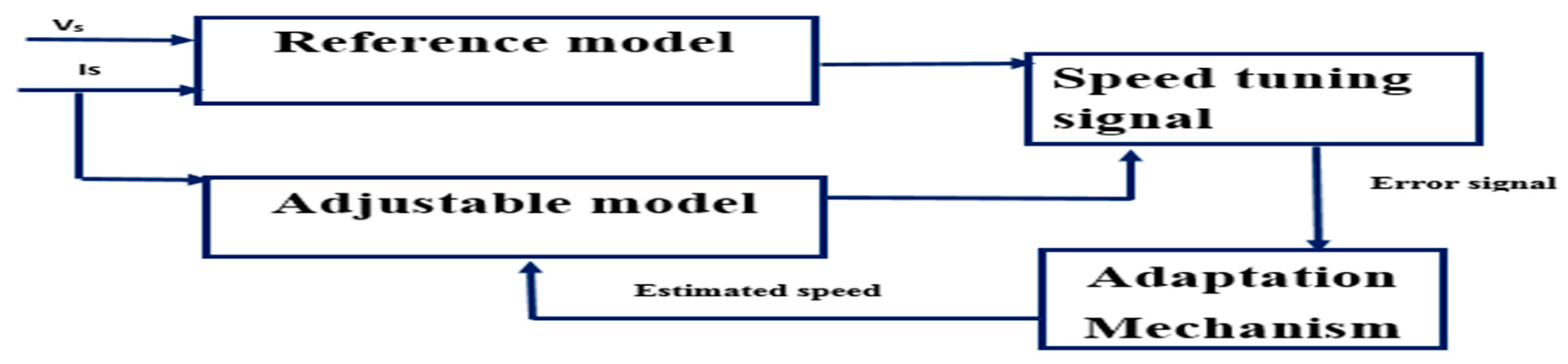
The model reference adaptive system (MRAS) estimators are the peak conservative method because of their modest structure and they have less associated calculation obligations than the other approaches. The elementary diagram of the MRAS contains an adjustable model, reference model, and an adaption mechanism. After the speed tuning, the error signal is given to the adaptation mechanism that is a neural network-based controller block. Here the output of both models is processed up to the errors linking the two models which depart to zero. The prototype accepts the voltage and current of the stator and determines the flux vector of the rotor. An adaptation mechanism with a neural network-based controller block is used to adapt the speed, so that the speed error is zero. The reference model equations are given by Equations (56) and (57).
The neural network-based Adaptive model equations are given by the following equations.
The error signal is given by Equation (65). It is being fed to the P-I regulator to obtain the speed signal (66).
The rotor speed is estimated from the estimated flux of the neural network-based model reference adaptive system.
2.5. Modified Extended Kalman Filter Method
R.E. Kalman proposed the method of an Extended Kalman filter (EKF) method in the year 1960. He put out his exalted paper describing an iterative answer to the digital-data linear trickling issues. An iterative estimator is a Kalman filter. This implies that only the evaluated state from the precedent time step and the measurement of current are required to tally the evaluation for the present state. In contradiction to bundle guesstimation methods, no background of observations and evaluation is compulsory. It is bizarre in being solely a time domain filter. The Kalman filter has two incisive phases: predict and update. The forecast phase manipulates the state evaluation from the preceding time step to outgrow an evaluation of the state at the current time step. In the upgraded phase, calculated data at the prevailing time step is utilized to clarify this prophecy to appear at a recent, (hopefully) more authentic state estimate, again for the current time step. In the collected works, a trendy technique for the data guesstimation of IM is the EKF. Typical ambiguity and nonlinearities innate to the induction motor are highly beneficial for the speculative identity of EKF. Using this technique, it is likely to develop the networked approximation of states while acting on the concurrent interconnection of data in a reasonably smaller time gap, also captivating the structure and measurement noises exactly into annals. This is the logic behind the EKF, which has developed an ample utilization spectrum in the sensor-less regulation of IMs, even if it is estimated intricacy. In this proposed method, the filter equation is altered by including a sliding hyper plane, and this will improve the performance of the system. The rotor voltage equations are given by (67).
From the voltage model of flux guesstimation, the rotor axis flux is given by
After eliminating isdr and isqr
Therefore, the desired state equation is given by
The dynamic equation is modified by altering the hyper plane, and the Filter equation is given by (83)
The speed adaptation algorithm is given by
The parameters of the induction motor illustrated in Table 1 are estimated for the 2.2 kW of the induction motor by a conventional direct current Resistance test, no load, blocked rotor test, and retardation test.
3. Simulation Results and Discussions
In sensor-less method regulation of an induction motor drive process the vector regulation without a speed sensor. For closed loop operations, the speed encoder is mandatory in both decoupling and scalar regulation drive. In the vector regulation with indirect form, a signal of speed is mandatory for the entire operation. A speed encoder is objectionable in the drive as it adds rate and consistency snags beyond the requirement for shaft enlargement and the mounting arrangements. It is important to evaluate the wave of speed from the currents and voltages of a machine terminal with the Digital signal processor (DSP). However, the guesstimation is commonly intricate and profoundly reliant on the parameters of the machine. While the regulation of without-sensor drives are free at this time, the change in parameter, predominantly closer to zero speed, enacts a provocation in the exactness of speed guesstimation [21].
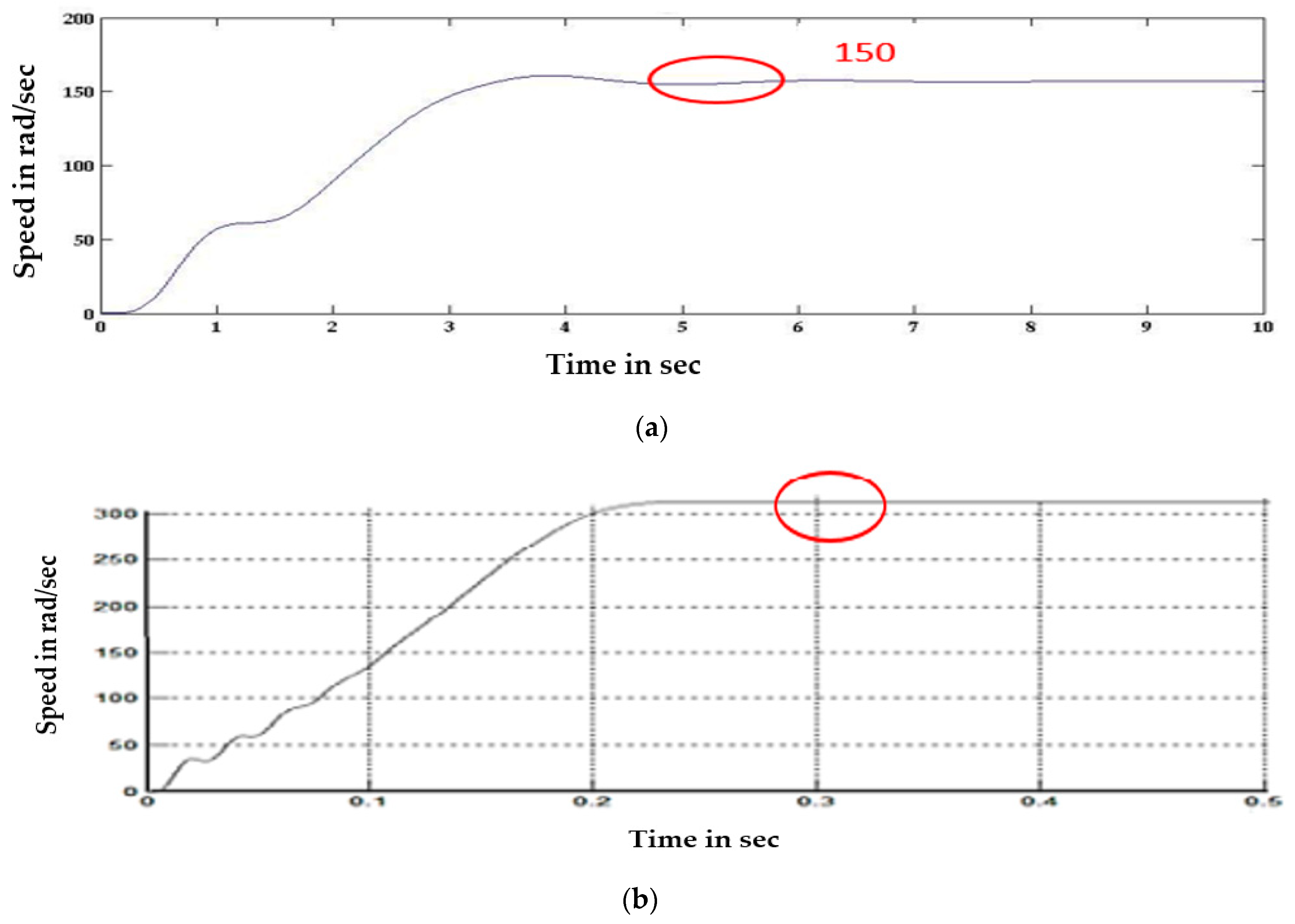
For large routine, changeable speed solicitations, the poly-phase asynchronous motors are used broadly because of having less rate, powerfulness, and less maintenance, and thus, they substitute the direct current motor drives. To achieve better torque and efficiency, the speed regulation of the induction motor is important. The dynamic modelling of a quinary phase induction motor is simulated in Matlab software. The phase voltages are converted into d-q axis voltages in three phases to a two phase lock. The speed and torque of the quinary phase induction motor have been estimated. The dynamically modelled induction motor in the quinary phase has 66% reduced torque pulsations and better linearity in the speed of the rotor, and also speed has been increased by 50% when compared to the induction motor in three phases as illustrated in Figure 1 and Figure 2 and Table 2.
3.1. Conventional Direct Synthesis Method
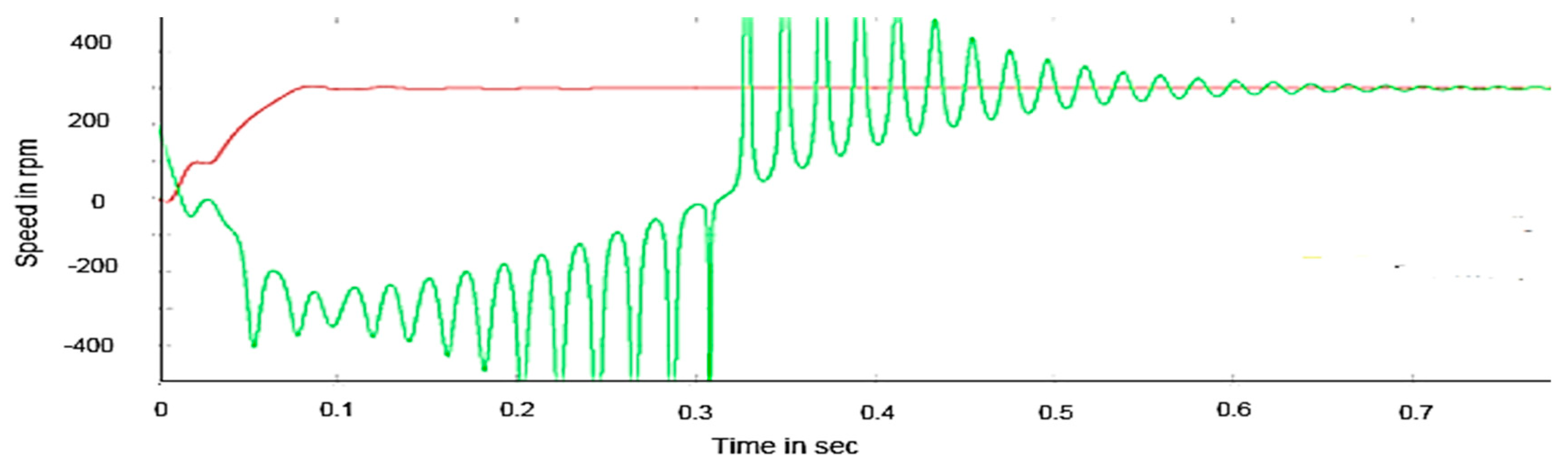
The speed guesstimation of the quinary phase induction motor using the direct synthesis method has been executed. The direct axis and quadrature axis fluxes are obtained using a current model block. The speed of the quinary phase motor has been approximated using the direct synthesis method. It can be seen that there is some difference between the estimated value and the reference value, so the accuracy of this method is low. Some speed pulsations of high magnitude are also present in the estimated speed. The estimated speed obtained using the direct synthesis method and reference speed has been demonstrated in Figure 3.
3.2. Neural Network Based Model Reference Adaptive System
The speed guesstimation using MRAS is executed in MATLAB software. The d and q axis voltages and currents obtained from dynamic model block [22] are fed to MRAS regulation, and the estimated speed is feedback to the adjustable model as shown in Figure 4.
The estimated speed of the quinary phase induction motor obtained using the MRAS method and the reference speed of the motor is demonstrated in Figure 5. The speed of the quinary phase motor has been approximated using the Model Reference Adaptive System method. It is observed that the estimated value and reference values are almost the same, thus offering good accuracy in guesstimation.
3.3. Modified Luenberger Observer Technique
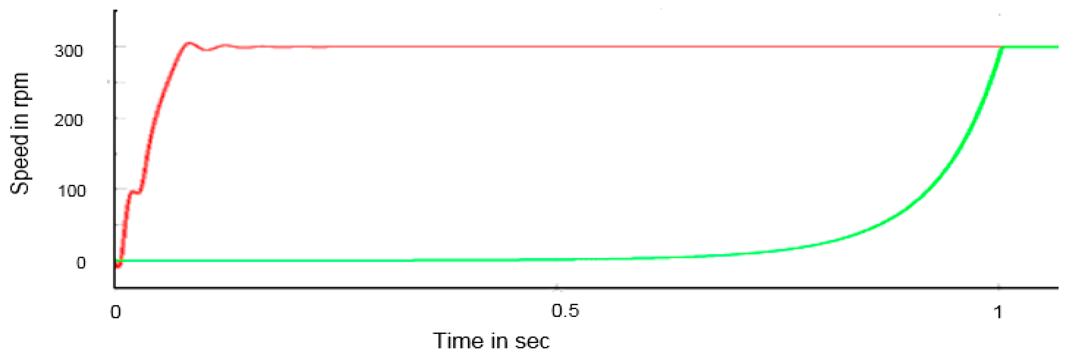
The speed guesstimation using the Luenberger observer method is executed in MATLAB software. This is illustrated in Figure 6. The speed response from the speed estimation using a Luenberger observer results in a small steady state error of 9 rpm, and the settling time took more than 2 s, which is high compared to all other methods.
3.4. Modified Extended Kalman Filter
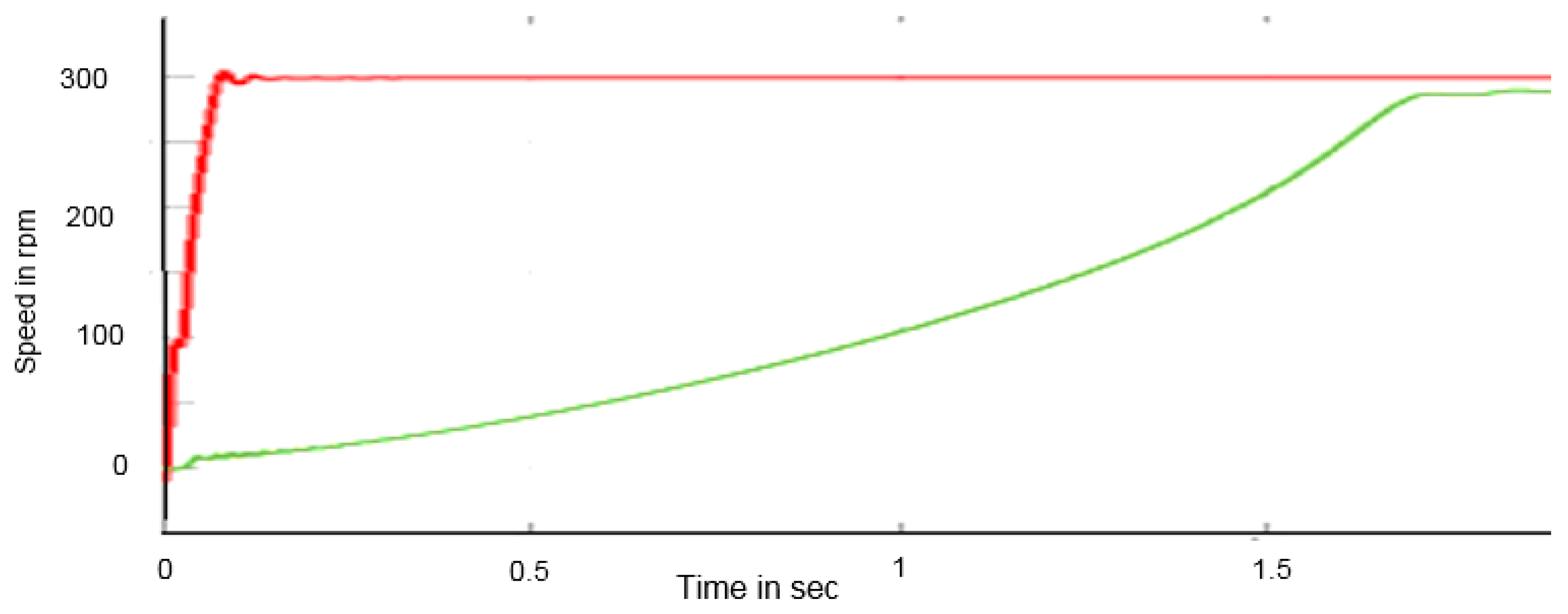
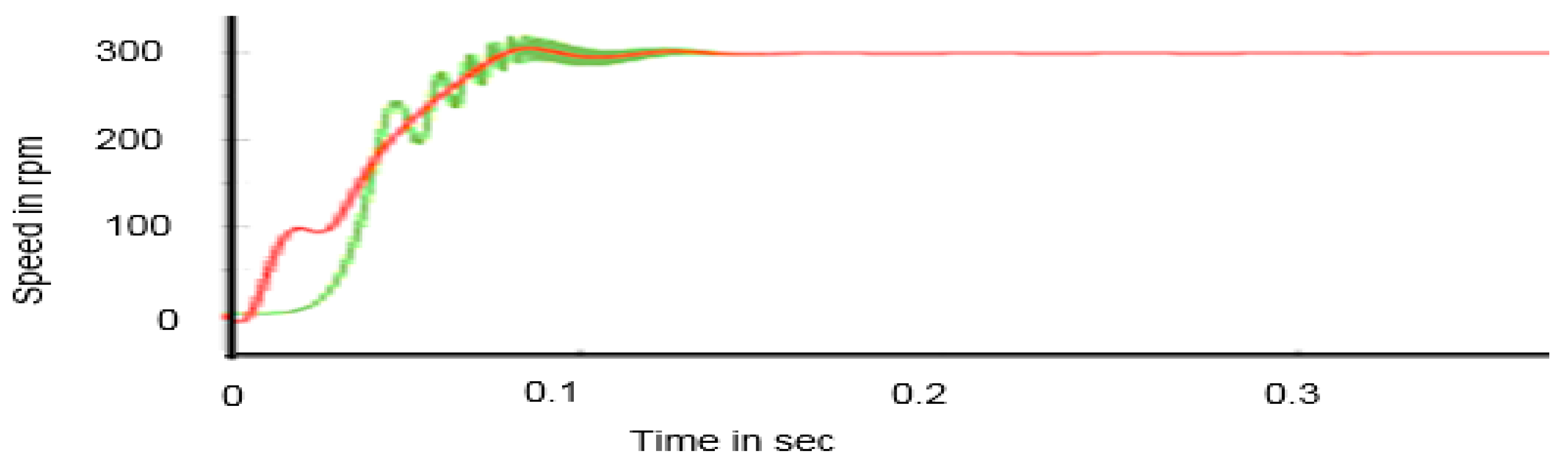
The speed guesstimation using the Kalman Filter method is being executed in MATLAB software. It can be observed from Figure 7 that the steady state error becomes zero and the settling time is also reduced drastically.
Speed pulsations of high magnitude are being observed in the estimated speed obtained by the direct synthesis method, which is not desirable. The rotor speed has been estimated using the direct synthesis method, model reference adaptive system, Luenberger observer method, and Kalman filter method. From the transient analysis, for the estimated speed obtained using these methods, the accuracy is better for the Kalman filter method because a steady-state error is zero and also the settling time is minimum compared to the other methods, so the speed reaches a stable state quickly. The Kalman filter enjoys very low settling time compared to all the above-mentioned guesstimation techniques that are depicted in Table 3.
The extended Kalman filter is the most popularly used observer in induction motor drive due to its nonlinearities and robustness of parameter variations. Conventionally, the covariance matrix and the parameters are tuned by a trial and error method. Due to the trial and error method, complexity and computational time is high. Based on the obtained model of a modified, extended Kalman filter, the computational time has been reduced.
4. Speed Deviation and Torque Ripple Reduction of Induction Motor Drive in Parallel Using Extended Kalman Filter
It is observed in both the simulation and hardware that the speed control of the induction motor is a challenging problem in the absence of a power electronics component [23,24]. In the proposed method, the induction motor with estimated parameters for sensor-less drive is analysed and compared with a conventional space vector modulation-based induction motor drive with a speed sensor. As no sensors are used, it makes the system more rugged, stable, less costly, and reduce in size. The two bogies setup where considered in this proposed method for electric traction locomotive application.
The speed of the five phase induction motor is estimated by the direct synthesis method, modified model reference adaptive system, Luenberger observer, and extended Kalman filter. From the above-mentioned speed estimation techniques, the extended Kalman filter has better performance than the other three methods. The speed and torque performance of the proposed method were analysed under the change in stator resistance, rotor resistance, low speed, and low inertia and compared with the conventional method. Here the proposed method is considered for electric traction locomotive application.
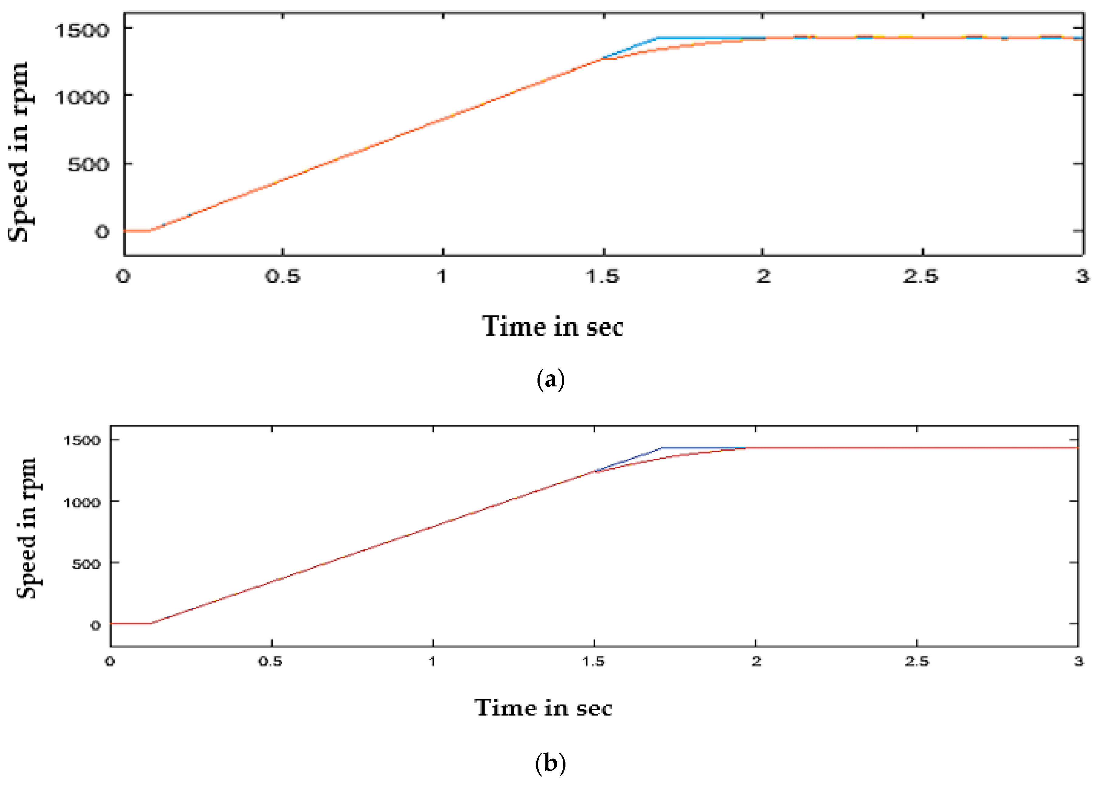
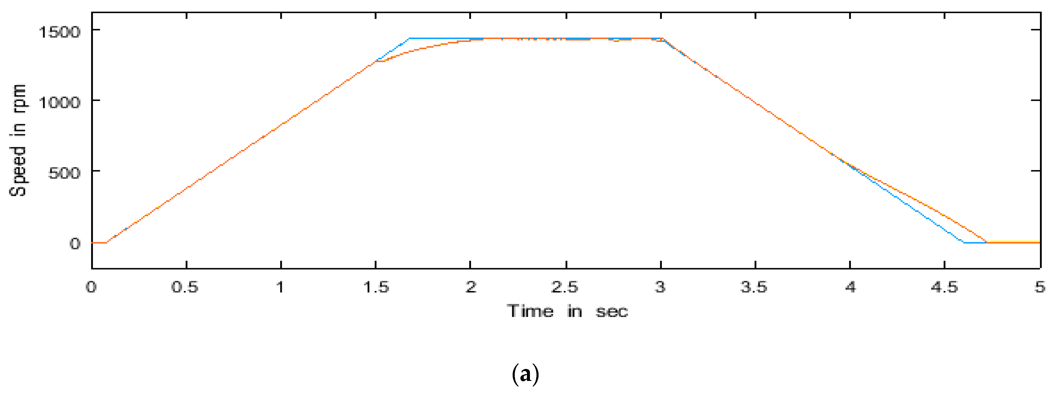
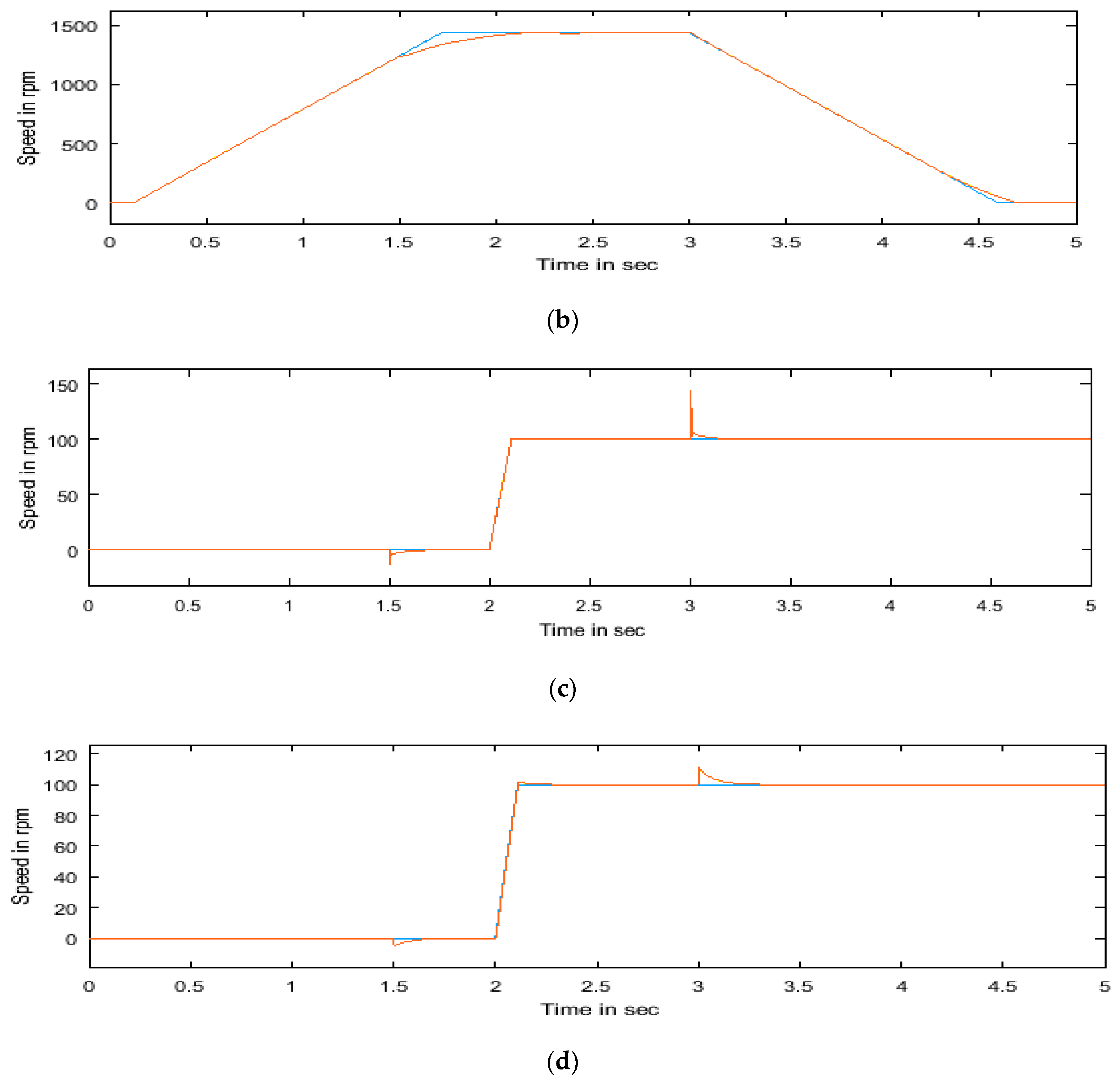
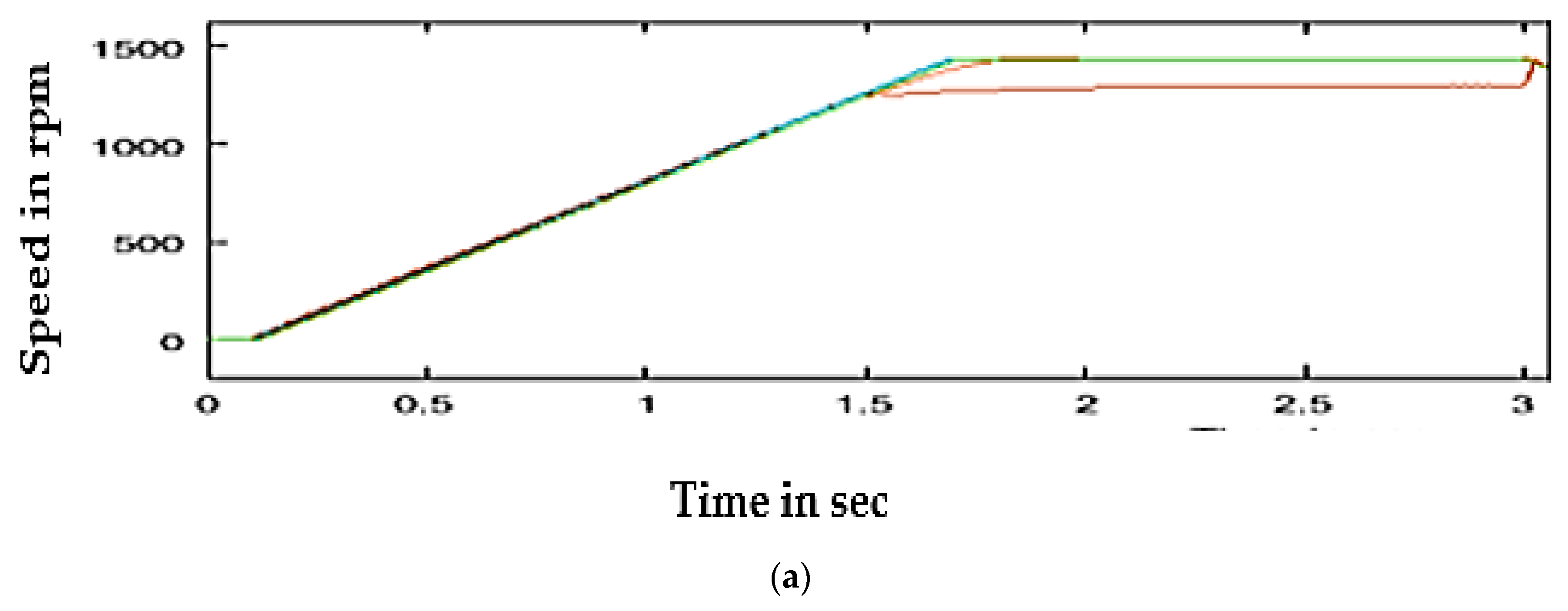
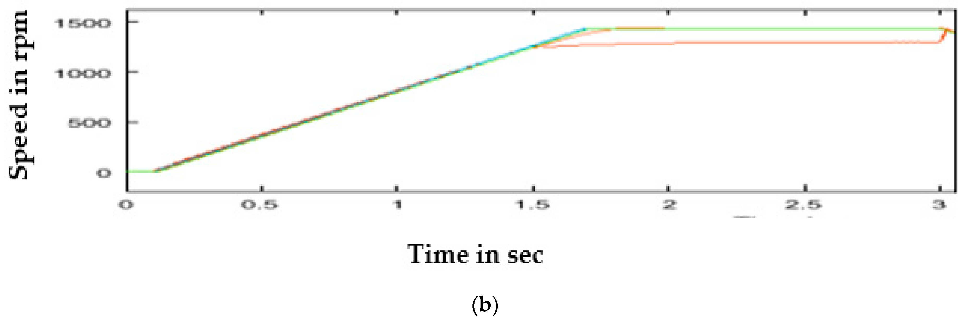
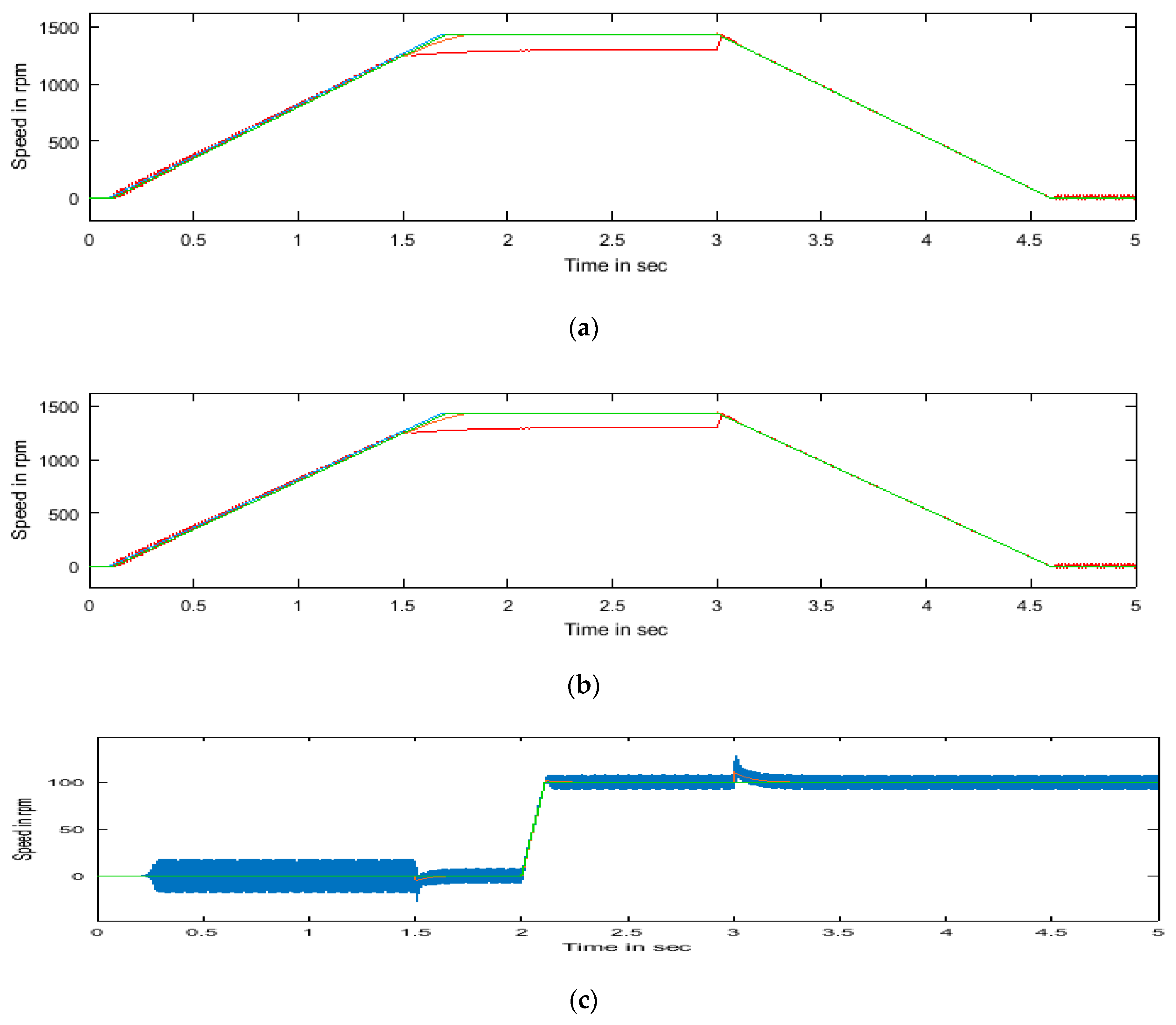
The speed response of the proposed method under normal conditions and parameter variations is shown in Figure 8 and Figure 9 respectively. In the rotor speed curve, the reference speed represented in yellow colour is matched to the estimated speed represented in red colour, and the actual speed is displayed in blue colour. The speed response of the conventional method under normal condition and parameter variations is as shown in Figure 10 and Figure 11 respectively. The speed error is far less in the proposed method, and it is robust to parameter variation compared to the conventional method. The speed error has been reduced by 70% in the proposed method compared to the conventional method.
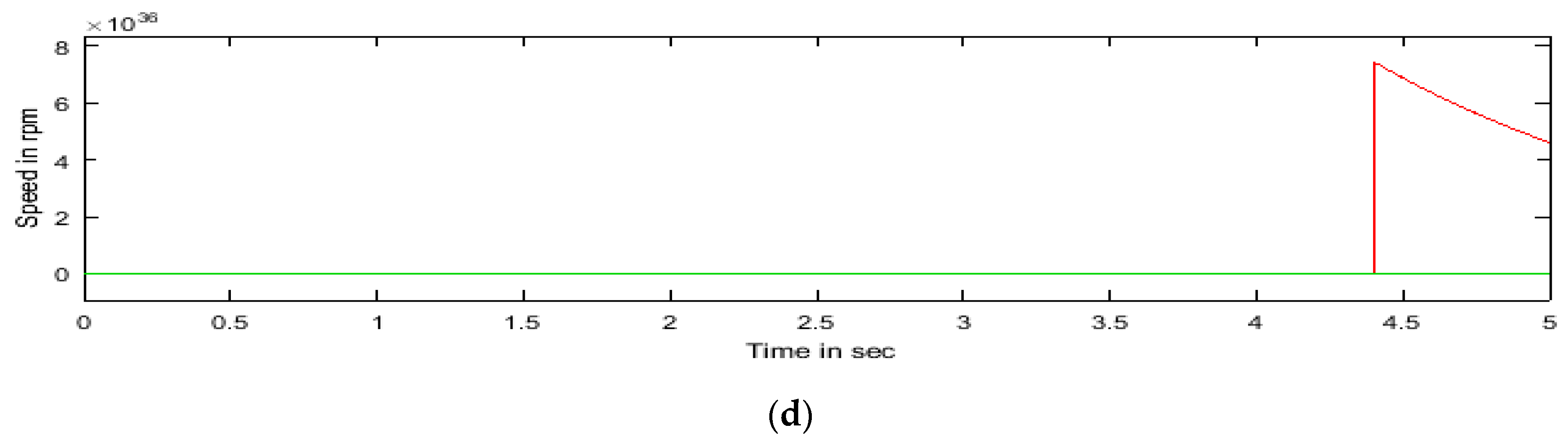
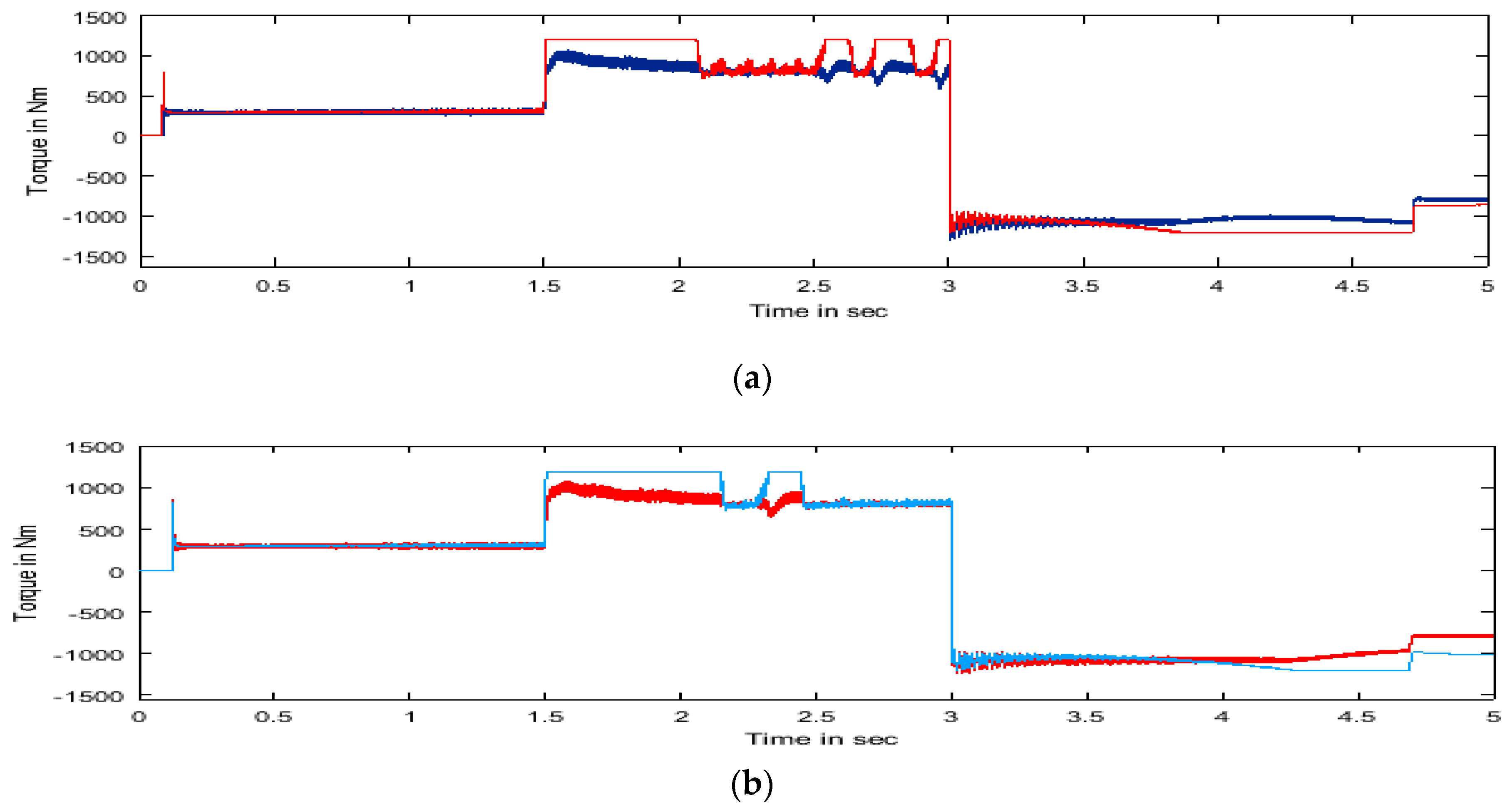
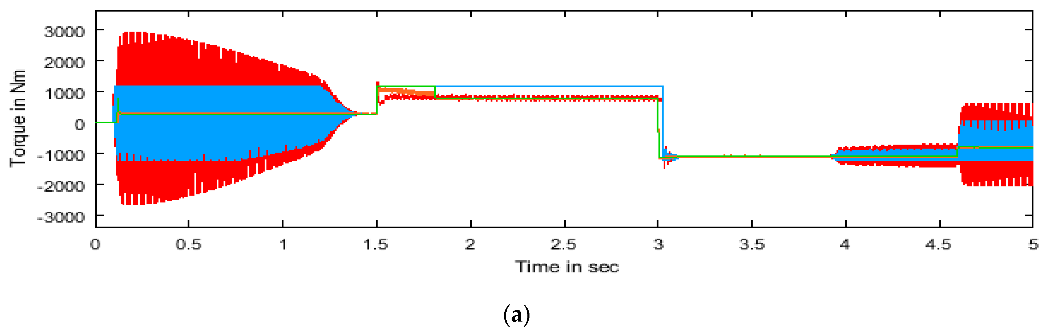
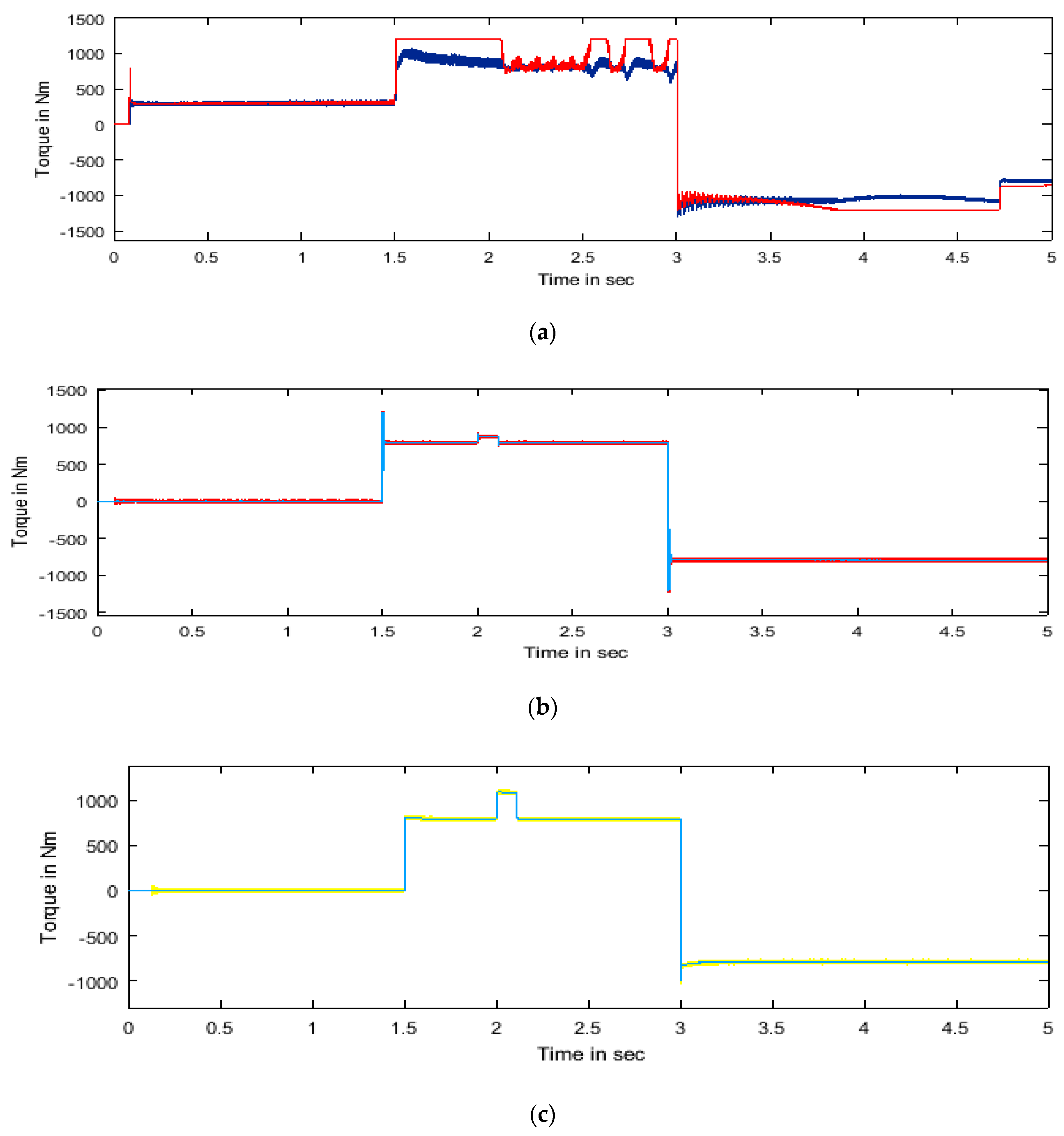
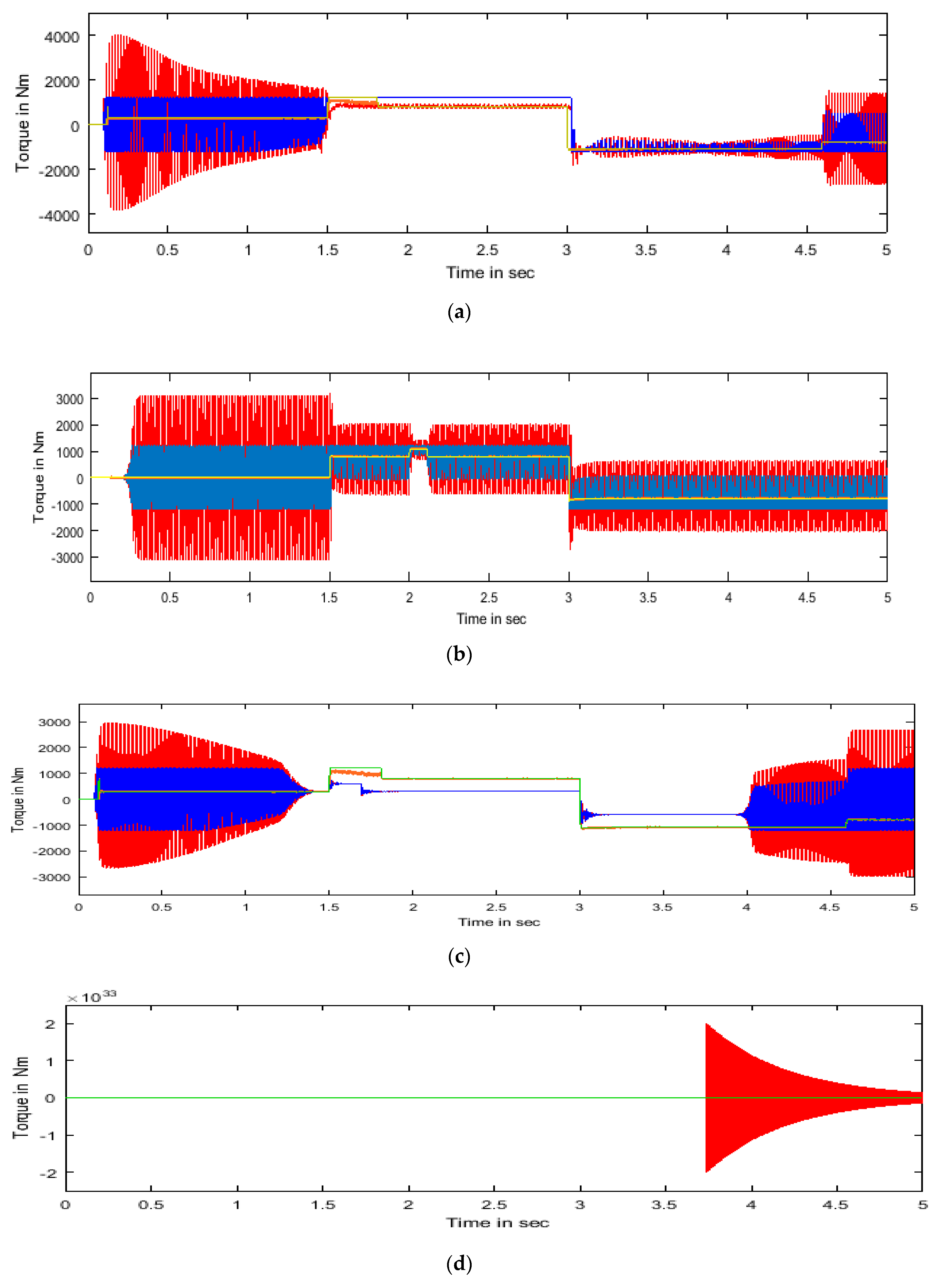
For the rotor speed, curve deviation is large compared to the proposed method. In the electromagnetic torque curve, the torque ripple is less in the proposed method compared to the conventional method as demonstrated in Figure 12, Figure 13, Figure 14 and Figure 15 respectively. The torque ripple is reduced by 85% in the proposed method compared to the conventional method.
The robustness of the proposed extended Kalman filter-based sensorless induction motor drive is compared with the conventional method. The robustness of the proposed method is proved by varying the stator resistance, rotor resistances, inertia, and step change in speed; also, under the low-speed region, it is proved that even though parameters varied, the performances are not affected compared to the conventional method.
Inference of Result
In the proposed method, the torque ripple is reduced by 85% and speed deviation reduced by 70% more than the conventional one. The performance is robust for parameter variations like a change in stator resistance, rotor resistance, low frequency, low inertia, the step change in speed, and low speed. The five phase induction motor has better performance than three phase induction motor in terms of torque ripple and speed error.
Speed pulsations of high magnitude are observed in the estimated speed obtained by the conventional direct synthesis method presented in B.K. Bose, which is not desirable in terms of response time compared to the proposed methods presented in the article. The conventional space vector modulated induction motor drive with a speed sensor has a high amplitude of torque ripple, ultra-low resolution rotary encoder, and it is difficult to realize proper control not robust for faulty environmental situations. The above-mentioned difficulties have been corrected in the proposed method of a sensor-less drive presented in this article.
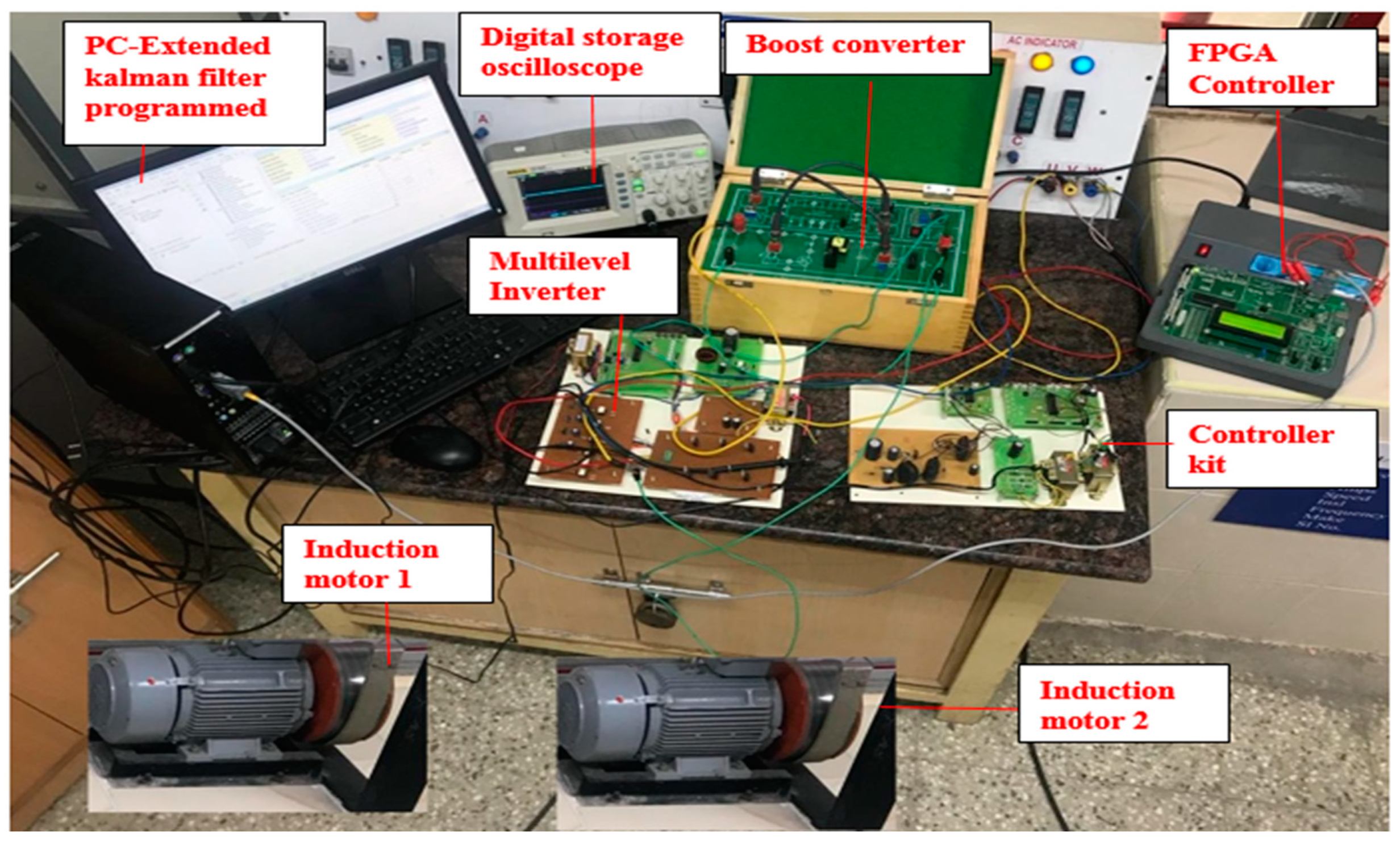
5. Hardware Results and Discussion
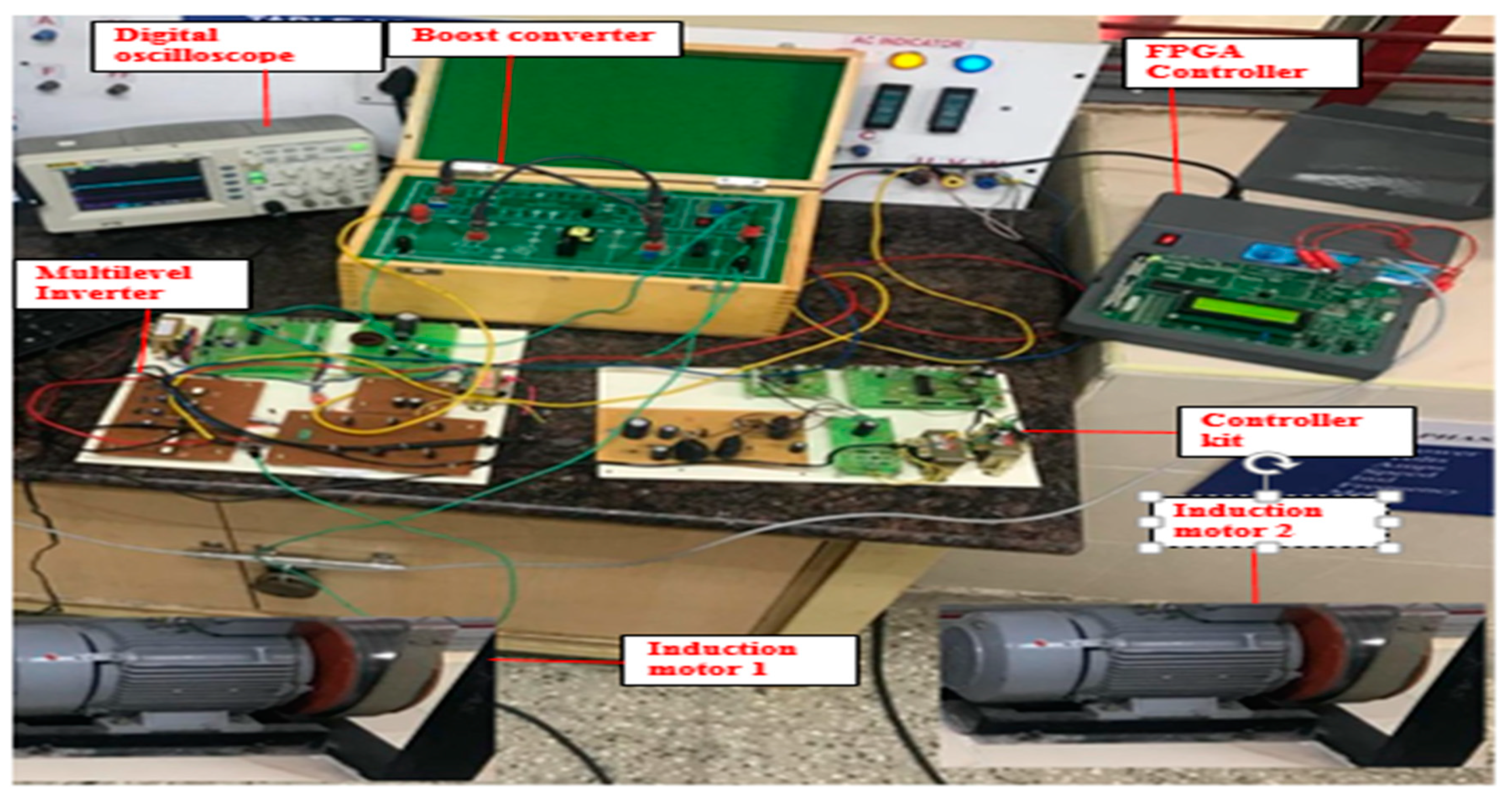
The performance acquired in the simulation is analysed experimentally in hardware setup also. The hardware setup for the sensor-based induction motor drive shown in Figure 16. The no-load test is performed on two motors connected in parallel. It is observed that the size and cost of the device are high. Thus, variable speed control becomes very difficult for this condition. The above-mentioned difficulties have been rectified in this proposed sensorless drive. The hardware setup for the sensorless drive is illustrated in Figure 17. Twenty-five percent of the size and cost of the system has been reduced in the proposed method.
6. Conclusions
The dynamically modelled quinary phase induction motor has reduced torque pulsations and better linearity in the rotor speed when compared to those of a three-phase induction motor. The rotor speed has been estimated using the conventional direct synthesis method, neural network-based model reference adaptive system, modified Luenberger observer, and extended Kalman filter methods. Comparing the estimated speed obtained using these methods, the accuracy is best for the Kalman filter method. Speed pulsations of high magnitude are observed in the estimated speed obtained by the direct synthesis method, which is not desirable. The Kalman filter employs very low settling time compared to all the above-mentioned guesstimation techniques. The minimization of speed error and torque ripple for the sensorless induction motor drive has been achieved. The hardware setup was implemented for the above-mentioned sensorless drive.
The current limiting factor of this proposed sensorless induction motor drive based on field-oriented control with proportional integral controller has ideal integration problems due to direct current offset, and, in addition, performance is not adequate at zero speed and low frequency. In future, the author will implement the modified model predictive control-based sensor-less induction motor drive for traction applications to improve the performance under zero speed and low-frequency conditions because of the speed characteristics of traction drive including the zero speed stat-up.
Author Contributions
Investigation, Software, Validation, Writing—original draft, Methodology, S.U.; Project administration, Supervision, Writing—review & editing, C.S.; Resources, S.P.
Funding
The research received no external funding.
Conflicts of Interest
The authors declare no conflict of interest.
References
- Echavarria, R.; Horta, S.; Oliver, M. A three phase motor drive using IGBTs and constant V/F speed control with slip regulation. In Proceedings of the IEEE International Power Electronics Congress, San Luis Potosi, Mexico, 6–19 October 1995. [Google Scholar] [CrossRef]
- Ho, T.J.; Chang, C.H. Robust speed tracking of induction motors: An arduino-implemented intelligent control approach. Appl. Sci. 2018, 8, 159. [Google Scholar] [CrossRef]
- Suwankawin, S.; Somboon, S. A speed-sensorless IM drive with decoupling control and stability analysis of speed estimation. IEEE Trans. Ind. Electron. 2002, 49, 444–455. [Google Scholar] [CrossRef]
- Hinkkanen, M. Reduced-Order Flux Observers with Stator-Resistance Adaptation for Speed-Sensorless Induction Motor Drives. IEEE Energy Convers. Congr. Expo. 2009, 20, 1–11. [Google Scholar] [CrossRef]
- Holtz, J. Sensorless control of induction machines with or without signal injection. IEEE Trans. Ind. Electron. 2006, 53, 7–30. [Google Scholar] [CrossRef]
- Edelbaher, G.; Jezernik, K.; Urlep, E. Low-speed sensorless control of induction machine. IEEE Trans. Ind. Electron. 2006, 53, 120–129. [Google Scholar] [CrossRef]
- Castaldi, P.; Tilli, A. Parameter Estimation of Induction Motor at Standstill with Magnetic Flux Monitoring. IEEE Trans. Control Syst. Technol. 2005, 13, 386–400. [Google Scholar] [CrossRef]
- Sumith, Y.J.; Siva Kumar, S.V. Estimation of parameter for induction motor drive. IEEE Trans. Ind. Appl. 2012, 2, 1668–1674. [Google Scholar] [CrossRef]
- Stephan, J.; Bodson, M.; Chiasson, J. Real-time estimation of the parameters and fluxes of induction motors. IEEE Trans. Ind. Appl. 1994, 30, 746–759. [Google Scholar] [CrossRef]
- Abdel-khalik, A.S.; Ahmed, S.; Massoud, A. A five-Phase Induction Machine Model Using Multiple DQ Planes Considering the Effect of Magnetic Saturation. In Proceedings of the IEEE Energy Conversion Congress and Exposition, Pittsburgh, PA, USA, 14–18 September 2014; pp. 287–293. [Google Scholar] [CrossRef]
- Fnaiech, M.A.; Betin, F.; Capolino, G.A. MRAS applied to sensor-less regulation of a six phase induction machine. In Proceedings of the IEEE International Conference on Industrial Technology Version, Vina del Mar, Chile, 14–17 March 2010; pp. 1519–1524. [Google Scholar] [CrossRef]
- de Lillo, L.; Empringham, L.; Wheeler, P.W.; Khwan-On, S.; Gerada, C.; Othman, M.N.; Huang, X.Y. Multiphase power converter drive for fault-tolerant machine development in aerospace applications. IEEE Trans. Ind. Electron. 2014, 57, 575–583. [Google Scholar] [CrossRef]
- Levi, E. Multiphase Electric Machines for Variable-Speed Applications. IEEE Trans. Ind. Electron. 2013, 55, 1893–1909. [Google Scholar] [CrossRef]
- Guglielmi, P.; Diana, M.; Piccoli, G.; Cirimele, V. Multi-n-phase electric drives for traction applications. In Proceedings of the IEEE International Electric Vehicle, Florence, Italy, 17–19 December 2014; pp. 1–6. [Google Scholar] [CrossRef]
- Comanescu, M.; Xu, L. Sliding mode MRAS speed estimators for sensorless vector control of induction machine. IEEE Trans. Ind. Electron. 2006, 53, 146–153. [Google Scholar] [CrossRef]
- Riveros, A.; Yepes, A.G.; Barrero, F.; Doval-Gandoy, J.; Bogado, B.; Lopez, O.; Jones, M.; Levi, E. Parameter Identification of five phase Induction Machines with Distributed Windings. IEEE Trans. Energy Convers. 2012, 27, 1067–1077. [Google Scholar] [CrossRef]
- Levi, E. Advances in converter regulation and innovative exploitation of additional degrees of freedom for quinary phase machines. IEEE Trans. Ind. Electron. 2016, 63, 433–448. [Google Scholar] [CrossRef]
- Kazuya, A.; Toru, I.; Matsuse, K.; Shigeru, I.; Nakajima, Y. Characteristics of speed sensorless vector controlled two induction motor drive fed by single inverter. In Proceedings of the 7th International Power Electronics and Motion Control Conference, Harbin, China, 2–5 June 2012. [Google Scholar] [CrossRef]
- Subotic, I.; Bodo, N.; Levi, E. Single-phase on-board integrated battery chargers for EVs based on quinary phase machines. IEEE Trans. Power Electron. 2016, 31, 6511–6522. [Google Scholar] [CrossRef]
- Slemon, G.R. Modelling of induction machines for electric drives. IEEE Trans. Ind. Appl. 1989, 25, 1126–1131. [Google Scholar] [CrossRef]
- Ohyama, K.; Asher, G.M.; Sumner, M. Comparative analysis of experimental performance and stability of sensorless induction motor drives. IEEE Trans. Ind. Electron. 2006, 53, 178–186. [Google Scholar] [CrossRef]
- Usha, S.; Subramani, C.; Geetha, A. Performance Analysis of H-bridge and T-Bridge Multilevel Inverters for Harmonics Reduction. Inter. J. Power Electron. Driv. Syst. 2018, 9, 231–239. [Google Scholar] [CrossRef]
- Sengamalai, U.; Chinnamuthu, S. An experimental fault analysis and speed control of an induction motor using motor solver. J. Electr. Eng. Technol. 2017, 12, 761–768. [Google Scholar] [CrossRef]
- Ang, J.; Yang, Y.; Blaabjerg, F.; Chen, J.; Diao, L.; Liu, Z. Parameter identification of inverter-fed induction motors: A Review. Energies 2018, 11, 2194. [Google Scholar] [CrossRef]
Figure 1.
Speed response of dynamically modelled induction motor: (a) proposed five phase motor and (b) conventional three phase motor.
Figure 1.
Speed response of dynamically modelled induction motor: (a) proposed five phase motor and (b) conventional three phase motor.

Figure 2.
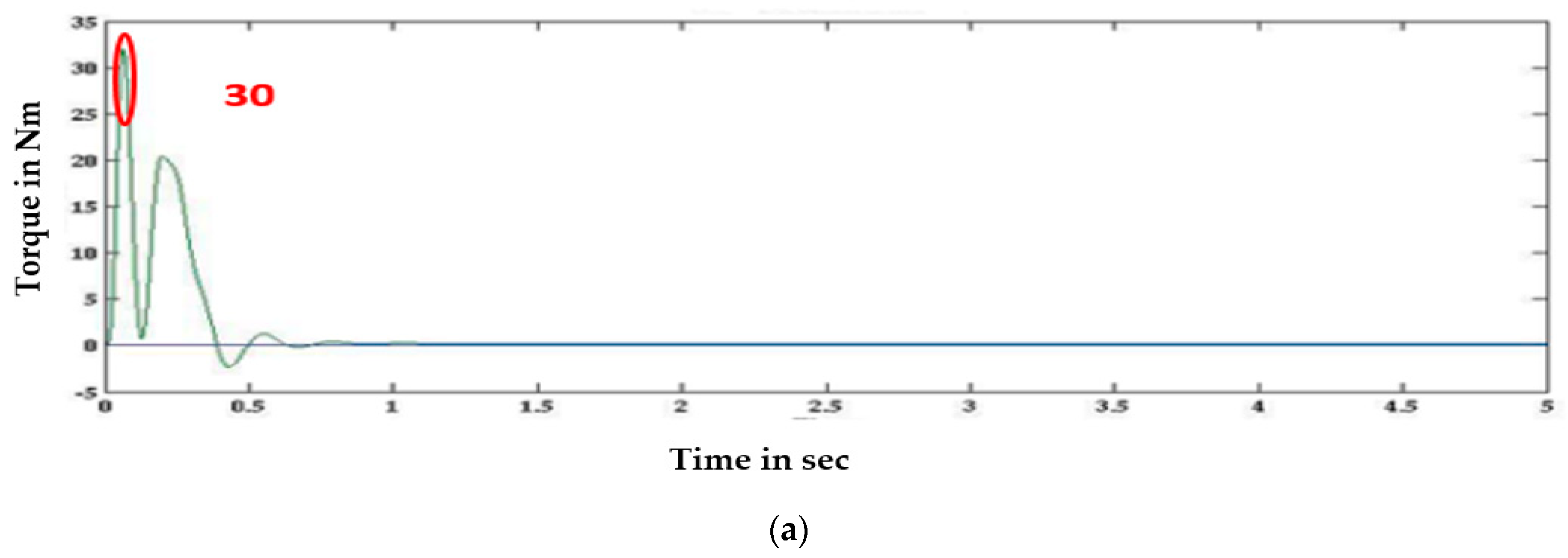
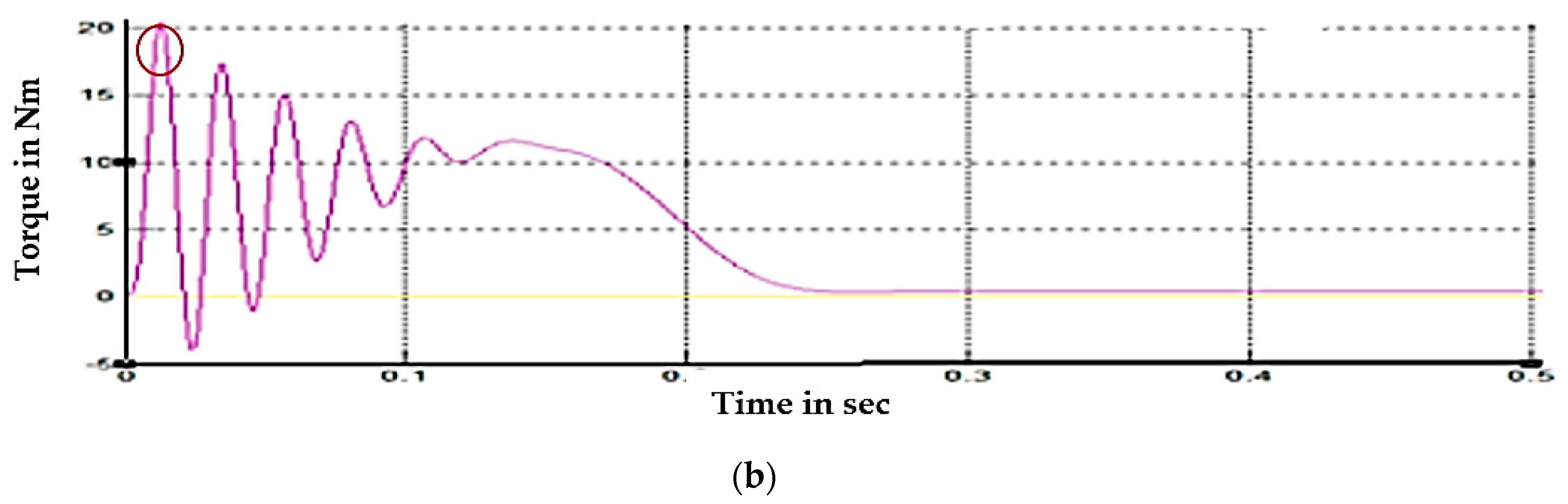
Torque response of dynamically modelled induction motor: (a) proposed five-phase motor and (b) conventional three-phase motor.
Figure 2.
Torque response of dynamically modelled induction motor: (a) proposed five-phase motor and (b) conventional three-phase motor.


Figure 3.
Estimated speed of a quinary phase induction motor obtained using Direct Synthesis Method.
Figure 3.
Estimated speed of a quinary phase induction motor obtained using Direct Synthesis Method.

Figure 4.
Model Reference Adaptive System.

Figure 5.
Estimated speed of the quinary phase induction motor obtained using Model Reference Adaptive Method.
Figure 5.
Estimated speed of the quinary phase induction motor obtained using Model Reference Adaptive Method.

Figure 6.
Estimated speed of the quinary phase induction motor obtained using a Luenberger observer method.
Figure 6.
Estimated speed of the quinary phase induction motor obtained using a Luenberger observer method.

Figure 7.
Estimated speed of the quinary phase induction motor obtained using Kalman Filter Method.

Figure 8.
Speed response of proposed sensorless induction motor drive under normal running conditions using Extended Kalman filter: (a) induction motor 1 and (b) induction motor 2.
Figure 8.
Speed response of proposed sensorless induction motor drive under normal running conditions using Extended Kalman filter: (a) induction motor 1 and (b) induction motor 2.

Figure 9.
Speed response of proposed sensorless induction motor drive under parameter variations using Extended Kalman filter: (a) change in stator resistance, (b) change in rotor resistance, (c) low speed, and (d) low inertia.
Figure 9.
Speed response of proposed sensorless induction motor drive under parameter variations using Extended Kalman filter: (a) change in stator resistance, (b) change in rotor resistance, (c) low speed, and (d) low inertia.


Figure 10.
Speed response of inverter-fed induction under normal running conditions using a conventional space vector modulation-based induction motor drive with a speed sensor: (a) induction motor 1 and (b) induction motor 2.
Figure 10.
Speed response of inverter-fed induction under normal running conditions using a conventional space vector modulation-based induction motor drive with a speed sensor: (a) induction motor 1 and (b) induction motor 2.


Figure 11.
Speed response of inverter-fed induction motor under parameter variations using a conventional space vector modulation-based induction motor drive with a speed sensor: (a) change in stator resistance, (b) change in rotor resistance, (c) low speed, and (d) low inertia.
Figure 11.
Speed response of inverter-fed induction motor under parameter variations using a conventional space vector modulation-based induction motor drive with a speed sensor: (a) change in stator resistance, (b) change in rotor resistance, (c) low speed, and (d) low inertia.


Figure 12.
Torque response of induction motor drive under normal conditions for proposed method: (a) induction motor 1 and (b) induction motor 2.
Figure 12.
Torque response of induction motor drive under normal conditions for proposed method: (a) induction motor 1 and (b) induction motor 2.

Figure 13.
Torque response of induction motor drive under normal condition for conventional method: (a) induction motor 1 and (b) induction motor 2.
Figure 13.
Torque response of induction motor drive under normal condition for conventional method: (a) induction motor 1 and (b) induction motor 2.


Figure 14.
Torque response of induction motor drive under parameter variations for proposed method: (a) change in stator resistance, (b) low speed, and (c) low inertia.
Figure 14.
Torque response of induction motor drive under parameter variations for proposed method: (a) change in stator resistance, (b) low speed, and (c) low inertia.

Figure 15.
Torque response of induction motor drive under normal conditions for conventional method: (a) change in stator resistance, (b) change in rotor resistance, (c) low speed, and (d) low inertia.
Figure 15.
Torque response of induction motor drive under normal conditions for conventional method: (a) change in stator resistance, (b) change in rotor resistance, (c) low speed, and (d) low inertia.

Figure 16.
Hardware setup for conventional method.

Figure 17.
Hardware setup for proposed method.

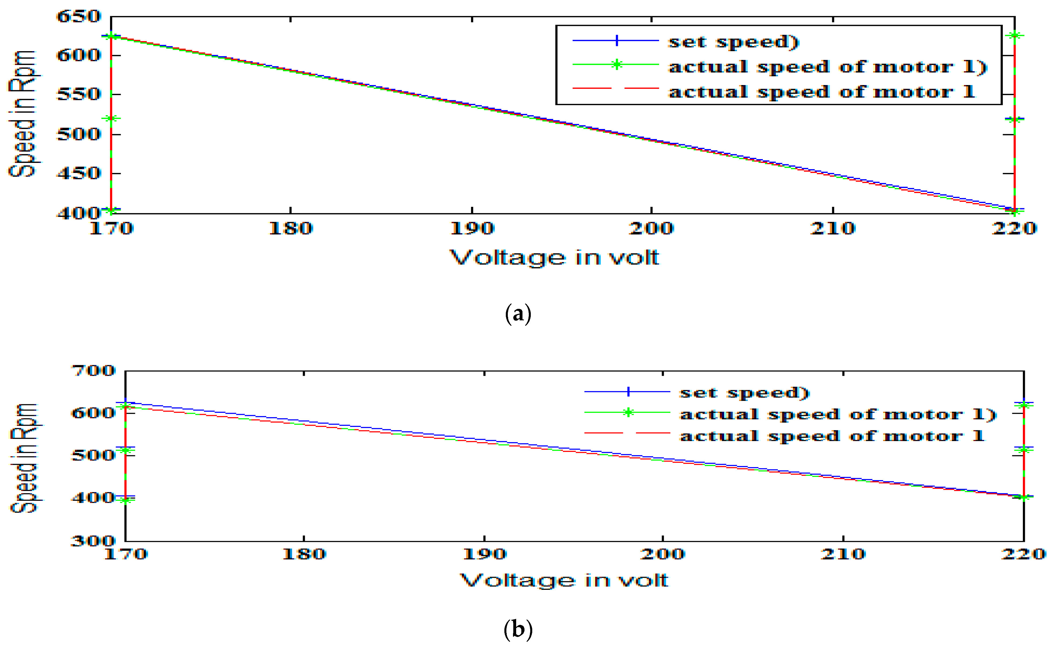
Figure 18.
Speed response of proposed method: (a) normal conditions and (b) parameter variations.

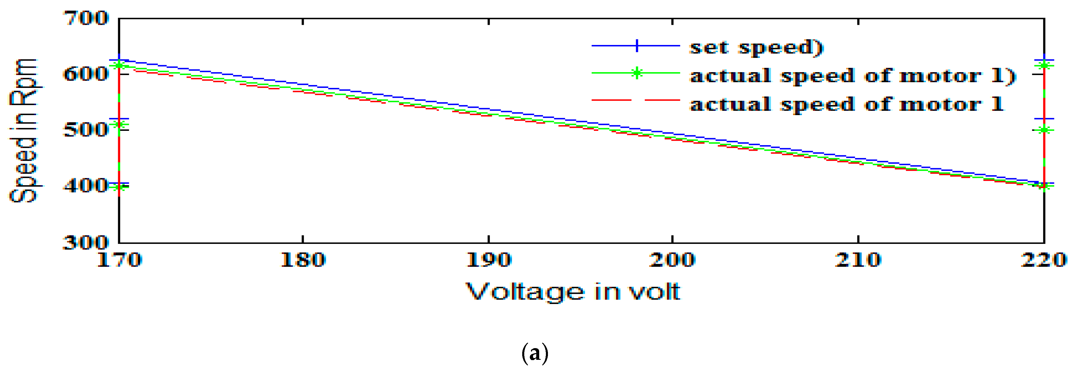
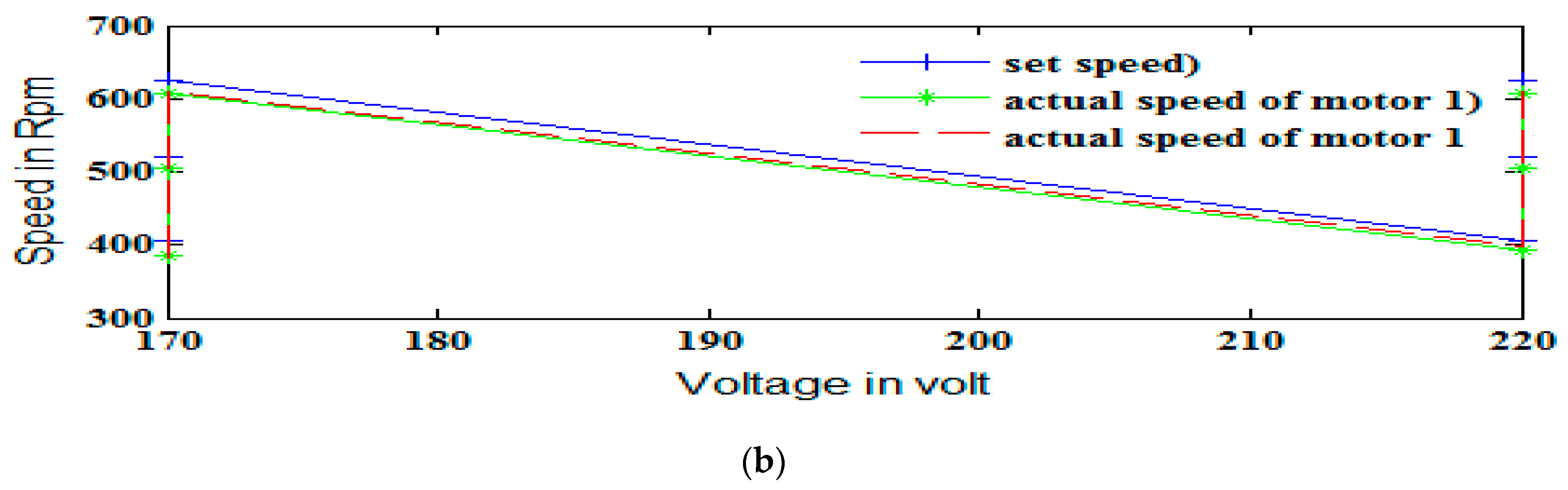
Figure 19.
Speed response of conventional method: (a) normal conditions and (b) parameter variation.
Figure 19.
Speed response of conventional method: (a) normal conditions and (b) parameter variation.


Table 1.
Machine parameters.
| Parameters | Values |
|---|---|
| power | 2.2 kW |
| Current | 4.4 A |
| resistance of stator | 6.6 ohms |
| Resistance of rotor | 5.5 ohms |
| Magnetising inductance | 0.454 H |
| Frequency | 50 Hz |
| No of poles | 4 |
| Moment of inertia | 0.011787 |
| Inductance of rotor | 0.475 H |
| Stator inductance | 0.475 H |
| torque | 2e−6 Nm |
Table 2.
Performance comparison of three- and poly-phase induction motor.
| Three-Phase Induction Motor | Poly-Phase Induction Motor | ||||
|---|---|---|---|---|---|
| Speed in rad/s | Setting Time of Speed in s | Amplitude of Torque Ripple in Nm | Speed in Rad/s | Setting Time of Speed in s | Amplitude of Torque Ripple in Nm |
| 150 | 2.5 | 30 | 300 | 0.2 | 20 |
Table 3.
Comparison of the guesstimation techniques by time domain analysis.
| Rise Time (s) | Settling Time (s) | Delay Time (s) | Steady State Error | Peak Overshoot (%) | |
|---|---|---|---|---|---|
| Model Reference Adaptive System | 1 | 1 | 0.9 | 0 | 0 |
| Luenberger Observer Method | 1.5 | 2 | 1.25 | 9 | 7 |
| Kalman Filter Method | 0.03 | 0.15 | 0.4 | 0 | −3.34 |
Table 4.
Speed response of conventional method under normal conditions.
| Voltage (V) | Current (A) | Actual Speed (motor 1) (rpm) | Actual Speed (motor 2) (rpm) |
|---|---|---|---|
| 170 | 0.9 | 400 | 400 |
| 0.9 | 512 | 519 | |
| 0.9 | 615 | 610 | |
| 220 | 1.2 | 415 | 415 |
| 1.2 | 525 | 520 | |
| 1.3 | 627 | 627 |
Table 5.
Speed response of conventional method under parameter variations.
| Voltage (V) | Current (A) | Set Speed (rpm) | Actual Speed (motor 1) (rpm) | Actual Speed (motor 2) (rpm) |
|---|---|---|---|---|
| 170 | 0.9 | 425 | 395 | 393 |
| 0.9 | 540 | 514 | 518 | |
| 0.9 | 635 | 608 | 610 | |
| 220 | 1.2 | 425 | 400 | 398 |
| 1.2 | 540 | 526 | 530 | |
| 1.3 | 635 | 626 | 622 |
Table 6.
Speed response of proposed method under normal conditions.
| Voltage (V) | Current (A) | Set Speed (rpm) | Actual Speed (motor 1) (rpm) | Actual Speed (motor 2) (rpm) |
|---|---|---|---|---|
| 150 | 0.8 | 425 | 425 | 421 |
| 0.8 | 540 | 538 | 538 | |
| 0.8 | 635 | 630 | 630 | |
| 200 | 1.2 | 425 | 425 | 425 |
| 1.2 | 540 | 538 | 539 | |
| 1.3 | 635 | 635 | 635 |
Table 7.
Speed response of proposed method under parameter variations.
| Voltage (V) | Current (A) | Set Speed (rpm) | Actual Speed (motor 1) (rpm) | Actual Speed (motor 2) (rpm) |
|---|---|---|---|---|
| 170 | 0.9 | 425 | 424 | 424 |
| 0.9 | 540 | 540 | 540 | |
| 0.9 | 635 | 631 | 635 | |
| 220 | 1.2 | 425 | 420 | 420 |
| 1.2 | 540 | 535 | 535 | |
| 1.3 | 635 | 635 | 635 |
© 2019 by the authors. Licensee MDPI, Basel, Switzerland. This article is an open access article distributed under the terms and conditions of the Creative Commons Attribution (CC BY) license (http://creativecommons.org/licenses/by/4.0/).
Share and Cite
MDPI and ACS Style
Usha, S.; Subramani, C.; Padmanaban, S. Neural Network-Based Model Reference Adaptive System for Torque Ripple Reduction in Sensorless Poly Phase Induction Motor Drive. Energies 2019, 12, 920. https://doi.org/10.3390/en12050920
AMA Style
Usha S, Subramani C, Padmanaban S. Neural Network-Based Model Reference Adaptive System for Torque Ripple Reduction in Sensorless Poly Phase Induction Motor Drive. Energies. 2019; 12(5):920. https://doi.org/10.3390/en12050920
Chicago/Turabian StyleUsha, S., C. Subramani, and Sanjeevikumar Padmanaban. 2019. "Neural Network-Based Model Reference Adaptive System for Torque Ripple Reduction in Sensorless Poly Phase Induction Motor Drive" Energies 12, no. 5: 920. https://doi.org/10.3390/en12050920
Note that from the first issue of 2016, this journal uses article numbers instead of page numbers. See further details here.