OSeMOSYS-PuLP: A Stochastic Modeling Framework for Long-Term Energy Systems Modeling †

Department of Energy Technology, KTH Royal Institute of Technology, SE-100 44 Stockholm, Sweden
*
Author to whom correspondence should be addressed.
†
OSeMOSYS-PuLP: https://github.com/codeadminoptimus/OSeMOSYS-PuLP .
Energies 2019, 12(7), 1382; https://doi.org/10.3390/en12071382
Submission received: 20 February 2019
/
Revised: 29 March 2019
/
Accepted: 3 April 2019
/
Published: 10 April 2019
(This article belongs to the Section B: Energy and Environment)
Abstract
:Recent open-data movements give access to large datasets derived from real-world observations. This data can be utilized to enhance energy systems modeling in terms of heterogeneity, confidence, and transparency. Furthermore, it allows to shift away from the common practice of considering average values towards probability distributions. In turn, heterogeneity and randomness of the real-world can be captured that are usually found in large samples of real-world data. This paper presents a methodological framework for an empirical deterministic–stochastic modeling approach to utilize large real-world datasets in long-term energy systems modeling. A new software system—OSeMOSYS-PuLP—was developed and is available now.It adds the feature of Monte Carlo simulations to the existing open-source energy modeling system (the OSeMOSYS modeling framework). An application example is given, in which the initial application example of OSeMOSYS is used and modified to include real-world operation data from a public bus transport system.
1. Introduction
1.1. Challenges and Opportunities
The world’s mean surface temperature is on a projected trajectory towards an increase of 2.5–7.8 °C compared to the pre-industrial era, if no additional efforts are made to reduce greenhouse gas (GHG) emissions [1]. This will presumably lead to tremendous impacts on human health and the ecosystem. Despite this dramatic outlook, global GHG emissions from fossil fuel burning, cement manufacturing, and gas flaring rose further by 2% per year over the period 2010–2014 [2]. The transport sector, in particular, accounted for 11% of this increase; consumed 27% of the total final energy use; and is projected to approximately double its fuel consumption by 2050 [1]. In contrast, some estimations state a reduction potential of 15–40% by 2050 compared to the baseline scenario [1]. This significant mitigation potential may be achieved if several measures are implemented such as: fuel switching, energy efficiency improvements, infrastructure development, behavior change, modal shift, and new policies [1,3,4]. Thus, the mitigation of climate change relies on the transformations of the energy system, including the transport system. That, however, implies comprehensive and fundamental changes at various levels.
The development of long-term energy planning scenarios is an indispensable tool to inform decision-makers about the potential benefits and drawbacks associated with a transformation. Therein, the field of energy systems modeling represents a cost-efficient and safe process to test and quantify impacts of new policies, measures, and targets on the economy, environment, and society. Modeling relies on the availability of data that is representative for the real world. Common practice is the use of aggregated data as input data for parameters in a model. Advantages are time-efficiency for both data collection and preparation; a single or few numbers that can potentially represent large amounts of data; reduction of complexity in a dataset and/or model; etc. Despite these clear advantages, drawbacks also exist such as: the dimensionality of the analysis is restricted to the aggregation level of the aggregated data; it is potentially impossible to trace back the aggregation to the original raw data; presumption for correctness of data preparation and aggregation calculations by others; etc. For example, average values (i.e., mean, median, mode) are commonly used in energy systems modeling as input data for parameters representing the energy demand side in a model. However, this simplified assumption neglects potential variations of parameters. Hence, this can result in missing heterogeneity and randomness of the real-world behavior in a model; limiting confidence in the aggregated data by the researcher of a study; limiting transparency of the input data for the model by the reader of a study; etc. Although, this was a non-exhaustive list of reasons, it compels efforts to overcome the said limitations that are inherited with the use of aggregated data. In comparison, probability distributions could represent more of the occurring variations from the real-world in a model. However, the determination of a probability distribution requires either much raw data to generate an empirical probability distribution, or the type of probability distribution must be explicitly stated along with its parametric values.
Meanwhile, recent open data movements gain scientific importance [5]. In addition, software and computer technologies evolve and can now support data preparation and analysis processes [6,7]. As a result, new opportunities arise through the access to non-aggregated data (i.e., raw data). Potential utilization of open real-world data could be: the development of more case-specific models; use of more heterogeneous input data (such as probability distributions instead of average values); and consequently, more heterogeneous output data. This might conceivably lead to richer and perhaps different sets of conclusions, each accompanied with a probability estimation, rather than one output dataset and one set of conclusions.
For instance, so-called “Intelligent Transport Systems” (ITS) [8] represent an example of the “Internet-of-Things” (IoT) concept [9]. Therein, physical vehicles are connected to other objects (e.g., a database) and exchange data. Through this, vehicle operation data are recorded, stored, and made available for analyses. This opens new possibilities to link energy and transport models; to develop scenarios that match more the reality; and eventually, to support decision-makers with more refined insights based on the actual raw data. Besides, the model’s user can be more involved in or do the data preparation and aggregation processes and hence, he/she is more familiar with the actual raw data behind the aggregated data. This might increase confidence in the analysis as well as enhance the transparency of modeling insights—starting at the raw data, to input data, to output data, to results, and eventually, insights. In addition, all this in a manner that is inherently tractable.
1.2. Rationale
This paper presents a methodological framework for an empirical deterministic–stochastic modeling approach to utilize large real-world datasets in long-term energy systems modeling. A new software system was developed, the so-called “OSeMOSYS-PuLP”. It is a new code implementation of the open source energy modeling system (the OSeMOSYS modeling framework) [10,11] with the substantial extension of Monte Carlo simulations (MCS). Other code implementations of OSeMOSYS (i.e., GNU MathProg, GAMS, and Python using the software library Pyomo [12,13]) have been extensively used for modeling and analysis of long-term energy planning scenarios in the scientific literature, e.g., see References [14,15,16,17,18,19,20,21]. However, those studies are limited in their usability to run MCS in an automated and convenient way. As a result, OSeMOSYS-PuLP overcomes this limitation and allows the analysis to consider and evaluate exogenous uncertainties of the model’s parameters using stochastic uncertainty analysis methods. A practical application example of a public bus transport system is presented to demonstrate the capabilities of OSeMOSYS-PuLP compared to the other code implementations. The input data was generated in form of an empirical probability distribution from real-world data, and hence, one example is provided on how OSeMOSYS-PuLP can be used.
The new software is ready-to-use for future research. Importantly, the new MCS extension for OSeMOSYS is not limited to any specific parameter. This means it is possible to choose an arbitrary parameter(s) to be considered in the MCS. This also enables an application of OSeMOSYS-PuLP for analyses having different scopes than this paper. Furthermore, it makes it possible to evaluate the overall impact of several combined exogenous uncertainties on the model’s output as well as stating the probability/likelihood estimated for each outcome.
1.3. Contributions
This paper makes three contributions: (i) The new software system OSeMOSYS-PuLP can support the development of more comprehensive and transparent long-term energy planning scenarios. These can support strategic data-driven decision-making within the areas of energy planning, transport planning, and policy design by allowing the inclusion of probability distributions to capture more heterogeneity and randomness of model parameters. For this, OSeMOSYS-PuLP is available for free and licensed under the Apache License Version 2.0 [22]. (ii) The methodological framework presents one way how to utilize large real-world datasets in long-term energy systems modeling with the aim to use raw data rather than aggregated data. This shall strengthen the confidence and transparency of the input dataset for both a model and the results from a model. (iii) The philosophy of open-data and open-source models is promoted, since the Python code of OSeMOSYS-PuLP is completely open-source designed, i.e., the modeling framework of OSeMOSYS-PuLP is open source, the Python programming language is open source, the default solver “COIN-OR Branch-and-Cut MIP (Mixed-Integer Programming) Solver” is open source, and the data sources used in this study are open and free.
Overall (i)–(iii): The paper contributes to the discourse of using large datasets in long-term energy systems modeling and strategic data-driven decision-making. Following this introduction, Section 2 describes aspects of data analytics for large real-world datasets in energy research with a focus on energy demand estimations for the transport sector. Section 3 provides an overview of the uncertainties and uncertainty quantification methods in energy systems modeling. Then, in Section 4, the methodological framework is described including the code implementation OSeMOSYS-PuLP. Moreover, the application example is presented as well as a summary of the data preparation is given. Then, Section 5 presents the results obtained from OSeMOSYS-PuLP. Section 6 reflects on the pros and cons of the methodological framework with respect to the use of large real-world datasets in long-term energy systems models and OSeMOSYS-PuLP. Lastly, in Section 7, the paper finishes off with a short summary, conclusions and recommendations for future work.
The Supplementary Material contains four files: (S1) a description of the data preparation and analysis; (S2) a short guide for OSeMOSYS-PuLP; (S3) the input dataset, and (S4) the output dataset of the application example. The files are available in the online version of the paper.
2. Utilization of Large Datasets in Energy Research
The term “big data” has been popularized over the past several years. Meanwhile, many datasets can be considered as large datasets and not “big data” sets. A large dataset still fits on an ordinary database and can be processed with a single computer (e.g., as in this study). In contrast, a big dataset requires another setup to be stored and processed, e.g., a multi-node cluster database for data storage and a computer cluster for data processing [23,24]. Nevertheless, processing of large datasets (i.e., not “big data”) can still require considerable computational power [25]. An example of how to process time-efficiently a large dataset on a single computer is “multiprocessing” [25]. It is a form of data management that simultaneously and in parallel processes several data files. Mounting research has been carried out around the utilization of large datasets and recently to support so-called “smart city” analysis. Definitions for the collective term “smart city” differ in the literature though, e.g., see several definitions listed in the study by Joglekar and Kulkarni (2017) [26]. Nevertheless, this term usually suggests inclusion of measurement and collection of real-world data from different sources and its analysis to enhance (energy) management, and therefore, life quality and efficiency. The ubiquitous monitoring, collection, and storage of vast amounts of data, while striving for open access, gives researchers new possibilities to make more refined assumptions in energy systems (as well as other types of) models. Thus, the digitalization of energy systems in cities and collaborative efforts among professionals from different disciplines could fundamentally change cities in their operation and management according to Zhang et al. (2017) [27].
Many of the published studies that use large real-world datasets focus on the energy demand of end users and can typically be allocated to two research foci: “residential buildings” and “urban transport”. One example is the provision of new services. Here, Moreno et al. (2015) [28] suggest the prediction of traffic congestion in advance of its actual occurrence and to provide an alternative route to avoid traffic jams. This prevents stop-and-go driving, and thus, saves energy and consequently, reduces emissions. A couple of studies have explicitly focused on estimating the energy demand of road vehicles using large real-world datasets. For instance, Gennaro et al. (2016) [29] monitored two conventional car fleets in the Italian provinces of Modena (52,834 cars) and Firenze (40,459 cars) during May 2011. The data was obtained from on-board logging devices that recorded GPS (Global Positioning System) coordinates, engine status, instantaneous speed, and driven distance. Their analysis focused on investing activity patterns of the two car fleets in urban areas and the emissions reduction potential when replacing conventional cars (i.e. a car that only has an internal combustion engine) by hybrid-electric cars (i.e. a car that has both an internal combustion engine and an electric motor) or battery-electric cars (i.e. a car that only has an electric motor). Overall, the study demonstrated the opportunity presented by utilizing real-world data to simulate different scenarios for the assessment transport policies in the European Union. Electric cars were also analyzed by Fetene et al. (2017) [30], who estimated the energy consumption rate (ECR) and all-electric range (AER) as a function of driver behavior, road type, and weather conditions. The data were collected from 741 drivers over a period of two years. The results showed that the ECR was 34% higher and AER was 25% shorter in the winter time than in the summer time. They further found a non-linear relationship between speed, acceleration, and ambient temperature on the ECR, whereas season and precipitation influenced linearly the ECR. The optimal operation was found to be at a speed between 45–56 km/h and an ambient temperature of 14 °C for battery-electric cars. These findings could consequently be considered in the operation of electric cars.
In addition to private cars, studies were published for taxis, especially for cases in China. Kan et al. (2018) [31] analyzed the spatio-temporal distribution of energy consumption and emissions for a cab fleet consisting of 6658 vehicles in the city of Wuhan. The data was collected on 6 May 2015. The findings from the data analysis generated deeper insights about the mechanisms and relationships of energy consumption and emissions depending on the vehicles’ activity in Wuhan’s road network. Similarly, Luo et al. (2017) [32] used large GPS datasets to analyze spatio-temporal energy consumption and emission patterns of 13,675 taxis in the city of Shanghai. The results identified areas and operation times in which both energy consumption and emissions peaks occurred during the day. These insights could be used to improve the planning of an urban infrastructure system in Shanghai, including improvements in the demand side for an energy-efficient transport sector and ultimately lowering its carbon footprint. Similar results were found by Cao et al. (2017) [33] who analyzed GPS data from taxis in the city of Guangzhou. The study divided the city in different area categories such as core areas, transition areas, and fringe areas. They found that the travel activity in transition areas was considerable higher during peak hours than in the other two areas. A case across different transport modes was investigated in the study by Guo et al. (2017) [34], who analyzed the operation data of taxis, buses, and the metro system in the city of Shanghai. They analyzed the benefits of having a public transport planning service for users that combines all three modes and jointly considers travel cost and travel time. By considering the three modes together, the service mitigates particular drawbacks that occur when using only one transport mode. These include the slow speeds of taxis and buses during peak hours; the large-meshed coverage of metro stations; or the high cost of taxis for long-distance travel. Thus, this service uses real-world data from the urban traffic system to facilitate for passengers a joint use of three transport modes aiming at a shorter and cost-efficient travel. Other expected benefits are claimed to be the mitigation of pressure on the urban road system, reduction of the total energy consumption, and an extended coverage of the city’s public transport system.
The aforementioned studies demonstrate the possibilities to utilize large datasets of and for transport systems at different scales. Concerning energy consumption, only the study by Fetene et al. (2017) [27] provides a distribution of the energy consumption estimation for the case of cars. Interestingly, the underlying dataset was closed though, i.e., it was not publicly accessible. Besides, more research for other cases than Europe and China would be useful to create multi-regional models or models across affiliated cities such as the C40 Cities [35]. Since international standardized driving cycles can considerably differ from the uniqueness of local driving patterns [36,37,38], there is a need to estimate energy consumption and to analyze driving cycles for various cases.
In summary, more research is needed to demonstrate the potential benefits of using large datasets in long-term energy system modeling. In this paper, the new software system OSeMOSYS-PuLP was developed which can use probability distributions to draw from distributions input data for model parameters, i.e., the input data are represented as distribution/s and then used in a long-term energy system model. Thus, the new tool makes exogenous quantification of uncertainties (more information on this topic follow in the next section) possible, and consequently, promotes transparency of a model’s outcome and drawn conclusions. An illustrative example is used for demonstration purposes: the public bus transport system of the city of Curitiba in Southern Brazil. This example also complements the previous studies by using an example of a public bus transport system instead of private cars and taxis. Noteworthy is the fact that only open-data and open-source tools were used in this paper. That gives more control over data quality and can enhance the trustworthiness and transparency of input datasets in a long-term energy system model. Overall, this paper provides a new modeling framework and uses a case study to contribute to the discourse of using large real-world datasets in long-term energy systems modeling.
3. Quantifying Uncertainties
An optimization model typically consists of an objective function, decision variables (or plainly said: “variables”), model parameters (“parameters”), constraints (“equations”), index sets (“sets”), and the input dataset. Many models are designed as techno-economic optimization models, i.e., a model that determines an optimal solution to a given problem by evaluating technology investment options, or in combination with other factors, e.g., social behavior, as done in the study by Moresino and Fragnière (2018) [39]. These optimization models are usually designed either deterministically (i.e., fixed values for parameters), stochastically (i.e., random values for parameters) or as hybrid models (i.e., a mix of fixed and random values for parameters). A deterministic model will always produce the same output data from the same input data, whereas a stochastic model will most likely produce different output data. With respect to the underlying input data, the topic of uncertainty must be considered, which is a multifaceted issue in energy systems modeling.
Assessing uncertainty is important to indicate the quality of a value for those who would like to use it and to understand its reliability [40]. Uncertainty can be evaluated and categorized in many ways. First of all, a measured value (and as used in an input dataset) and true value (as occuring in the real-world) can potentially differ due to imprecision of measurements or inaccuracy of measurement devices [40]. Moreover, measurements and values need to be explicitly described to prevent any form of ambiguity concerning use and interpretation [41]. Eventually, ambiguity in data or wordings can lead to different interpretations among different people based on their own knowledge background. Thus, elimination of ambiguity is highly desired, which can be a difficult task though. Thus, an imperfect definition can lead to vagueness in the communication of research findings [42].
Presuming a thorough review of measurement practices and definitions before a dataset is used, let us consider that such a dataset has got the status “as is” in an energy system modeling study. Then, uncertainty can be distinguished between endogenous and exogenous uncertainties. Endogenous uncertainty is caused during the model’s design. It is induced when assumptions in the model’s equation system are made by the model’s developer concerning relationships of variables and parameters. By comparison, exogenous uncertainty is caused during the model’s use. It is induced when assumptions in the model’s input data are made by the model’s user. Different analysis methods are available to quantify uncertainties as illustrated in the Uncertainty analysis matrix (UAM) in Figure 1. The methods are described in the following sub-sections with focus on deterministic models, because the considered OSeMOSYS modeling framework belongs to this category.
3.1. Endogenous Uncertainty in Deterministic Models
Scenario analysis often appears as a conceptual key element in scientific studies rather than to quantify explicitly the endogenous uncertainty in deterministic models by itself, e.g., as used by Chollacoop et al. (2015) [43]. Scenarios are developed in form of narratives, models are accordingly built and based on this, conclusions (often in the form of “insights”) for potential future outcomes are obtained and interpreted.
Another possibility to quantify endogenous uncertainty in deterministic models is to disclose the source code or its algebraic formulation. An open-source code allows the model’s user to review the assumptions made by the model’s developer and potentially estimate logical and numeric influences on the results. However, applied research fields lag particularly behind concerning both open-source models and open data [5]. For instance, only a few models are open source out of 96 models and simulation tools for long-term energy systems analysis that were identified by Hall and Buckley (2016) [44] in the case of the UK. Besides, Pfenninger et al. (2017) [5] stated as potential reasons limited guidelines to develop real-world energy systems as well as varying quality of heterogeneous data as potential reasons for the limited number of open source models. Both imply that there is a key limitation in the field of energy research. Only a few active academic open-source models have existed for more than a few years including Balmorel [45], TEMOA [46], and OSeMOSYS [10,11]. Preceded by DEECo in 2004, and GnuAE in 2005, OSeMOSYS—with an easy to decipher code base—sparked a new wave of open-source endeavors [47]. Noteworthy was an analysis by Groissböck (2019) [48], which concluded that only four (Switch, TEMOA, OSeMOSYS, and pyPSA) out of the 31 models that were analyzed in the study are mature enough for serious use. The evaluation was based on a function comparison.
3.2. Exogenous Uncertainty in Deterministic Models
Like open-source code, open data can contribute to greater transparency. It allows the reader of a study to review the assumptions made by the model’s user. Therefore, provision of the whole input dataset can support the objective tackling of exogenous uncertainty in the modeling process. Both allow repeatability that helps to improve the quality of science, promote effective collaboration between science and policy-making, increase productivity, and is relevant for societal debates [5].
Sensitivity analysis is another option. It quantifies the change of the model’s output data to the change(s) of one parameter or a combination of more parameters in the input data. This method is frequently used to test the robustness of findings, e.g., see References [49,50,51]. However, usually only one or a few parameters are tested. In contrast, Weijermars et al. [52] suggests performing an extensive sensitivity analysis accompanied with a clear explanation of the underlying methodology. This, it is argued, shall achieve a more careful and transparent appraisal of findings and drawn conclusions. Through combining methods to sift through large quantities of results and understanding their key determinants, hidden insights can be gained [53].
3.3. Limitations of A Deterministic Uncertainty Analysis
Scenario analysis, sensitivity analysis, and disclosure of both source code and input datasets are depicted options to provide more transparent insights and test the model’s assumptions and robustness. Yet, all come with the implicit assumption that the values for the parameters (including their variance) are “representative enough”. This implies an assignment of values to parameters before a model is actually run, and likewise, a resolution of uncertainty ex ante as pointed out by DeCarolis et al. (2017) [54]. For example, a critical and influential parameter is often the discount rate in techno-economic energy system models. It is used to estimate the present cost of investments to the time point(s) when the investments are made. Considering both that economic growth and energy consumption are non-linearly related [55] and that empirical findings actually show a negative relationship between economic growth and energy intensity [56], this complexity requires a clear justification for the assumed projection of the discount rate [57].
With reference to projections, the recent review by Debnath and Mourshed (2018) [58] illustrates a variety of available methods to forecast input data for parameters. They found that most forecasting methods are used to project energy demand and electrical load. Historical trends and the baseline year often serve as references to develop future projections. However, the assumption of baseline year data can significantly differ between studies and can lead to different conclusions as found by Yeh et al. (2017) [59]. Furthermore, a sensitivity analysis cannot quantify the uncertainty caused by random errors in the input data [49]. For instance, the two academic deterministic energy system modeling framework Balmore [45] and OSeMOSYS [10,11] typically (except Ref. [19]) assume perfectly forecasted demands and do not capture stochastic properties of their parameters [10,11,45]. Examples for varying parameters include solar power [60] and wind power [61] that both depend on weather conditions. In contrast, the TEMOA model can address these uncertainties due to its design for using stochastic programming and having the possibility to generate near-optimal solutions. Near-optimal solution generation takes into account heuristic principles to find a feasible solution through the means of approximation. However, as stated by the word “near-optimal”, the found solution does not necessarily give the “optimal” solution.
Evidently, uncertainties are ubiquitous in the modeling process on different levels and must be addressed through an uncertainty analysis to present transparent input data, results, and more comprehensive and robust conclusions. Since linking of different models to complement each other can be quite difficult, Timmerman et al. (2014) [62] proposed that it is more promising to extend an existing model instead. Therefore, in this study, the usability of the OSeMOSYS modeling framework is extended by the feature of Monte Carlo simulations to overcome its limitation concerning the stochastic behavior of parameters. For this, a stochastic uncertainty analysis for deterministic models is used as described next.
3.4. Stochastic Uncertainty Analysis for Deterministic Models
One way to quantify uncertainty from the stochastic behavior of parameters in deterministic models is the use of Monte Carlo simulations (MCS). Monte Carlo simulations draw a random value from a distribution associated with a selected parameter and assigns it to the parameter before the model is run. Then, the model is run and output data are obtained. This procedure is frequently repeated so that a probability distribution of the model’s result can be created and the probability for a certain outcome can be stated. This technique is not limited to only one parameter and can include an arbitrary but fixed number of parameters. In any case, the model’s user must either consider a probability distribution from the literature or make a reasonable assumption about the distribution. Or, the model’s user combines value estimations made in different studies by generating an empirical probability distribution based on those rather than calculating an average value out of all available values. Alternatively, if the model’s user has access to a large amount of data, either an empirical probability distribution (e.g., as it is done in this study in Section 4.3.1 and File S1 in the Supplementary Material) or a theoretical probability distribution could be generated and used to draw from it input data for a parameter. Although, the latter still comes with an exogenous uncertainty for the probability distribution, MCS still allows for the quantification of the probability for an outcome. As a result, a more transparent evaluation can be made, that potentially leads to a more comprehensive interpretation of findings by considering the uncertainty space [63] and more convincing conclusions.
The possibility of running MCS directly in a fully open source implementation of OSeMOSYS has not existed so far. Leibowicz (2018) [19] developed a stochastic version of OSeMOSYS using GAMS. However, GAMS is not fully open source. Other studies, e.g., the recent study by Martišauskas et al. (2018) [64] and Leibowicz (2018) [19], combined MCS tools with the OSeMOSYS modeling framework. However, the actual process to eventually run the models has been quite inconvenient. Thus, an automatic way would be desirable. In addition, this is possible with OSeMOSYS-PuLP now. It allows to run MCS in a convenient and automated way. This substantial extension particularly contributes to research about stochastic optimization and quantifying exogenous uncertainties in long-term energy systems models. The OSeMOSYS-PuLP and the application example are presented next.
4. Methodological Framework and Application Example
The methodological framework presents an empirical deterministic–stochastic modeling approach to utilize large real-world datasets in a long-term energy system model (Figure 2).
The empirical component is the use of real-world data as demonstrated in the practical example of the public bus transport system in the city of Curitiba in Southern Brazil. The deterministic component is use of the deterministically designed OSeMOSYS modelling framework. The stochastic component is the extension of the OSeMOSYS modelling framework by adding the feature of Monte Carlo simulations (MCS) through a new code implementation and embedding it into a larger software system—OSeMOSYS-PuLP. All steps of the methodological framework and analysis process are described in the following sub-sections, starting with an introduction to the OSeMOSYS modelling framework and OSeMOSYS-PuLP, and then followed by a description of the application example including data preparation and the input dataset.
4.1. OSeMOSYS Modeling Framework
At the beginning of an energy systems analysis, the abstraction of the real-world energy system is first sketched in form of a reference energy system (RES) [65]. The RES illustrates flows of energy sources at different stages in the energy system—from the energy sources extraction to the final energy use by services. The OSeMOSYS (Open Source Energy Modeling System) modeling framework represents one example that allows the consideration of all stages to model the RES. It is an open-source bottom-up modeling framework aiming at long-term energy systems planning and optimization [10,11,12]. The user defines a specific model by providing input data to parameters for energy demand, energy supply, energy and/or emission targets, techno-economics, capacity-building constraints, etc. The OSeMOSYS modeling framework has been widely used in scientific studies to generate outlooks and to enhance understanding concerning the impact of structural transformations in energy systems concerning economic, environmental, and social aspects, e.g., see References [14,15,16,17,18,19]. The structure and features of the OSeMOSYS modeling framework have been well described in the scientific literature, see References [10,11]. Other existing and widely used software tools belonging to the model family of energy system optimization models, e.g., MESSAGE [66] and TIMES [67], are similar in their structure and insight generation. However, most of the tools have fully or partially closed code. In contrast, the OSeMOSYS modeling framework and most existing code implementations are open source—from the equations to the default solver (e.g. the latter does not apply to GAMS). This allows a potential reuse such as was done in this study by coding the OSeMOSYS modeling framework with the Python software library PuLP [68] and embedding it into a wider software system consisting of other Python software libraries and any spreadsheet software that can read and write .xlsx files, giving together “OSeMOSYS-PuLP”.
4.2. OSeMOSYS-PuLP
The OSeMOSYS-PuLP was implemented and tested in Python 3.6.6 [69]. It consists of standard Python code as well as the Python software libraries: PuLP [68] for the linear optimization model; Pandas [70] for data handling; Numpy [71] for probability distribution functions; and xlrd [72] to create a spreadsheet file that can be opened with either Microsoft Excel [73], Apache OpenOffice Calc [74], LibreOffice Calc [75], or any other spreadsheet software that can read and write .xlsx files. The open-source mixed-integer programming (MIP) COIN-OR Branch-and-Cut MIP Solver was used by default as it is the default solver in PuLP [76]. Nevertheless, other common solvers are supported, too. More information about PuLP including utilizable solvers is available on the documentation website of PuLP in Reference [77]. Noteworthy is that OSeMOSYS-PuLP has some distinct differences compared to other existing code implementations such as GNU MathProg [78], GAMS [79], and Python-Pyomo [80,81] (all code implementations of the OSeMOSYS modeling framework are available in Reference [12]). The key differences are:
Firstly, the new feature of MCS adds a considerable extension of the functionality to the OSeMOSYS modeling framework. The user can choose between some predefined probability distributions (normal, triangular, uniform, choice), as well as has the possibility to add more specific probability distributions if needed, e.g., from Reference [82]. The input data for the probability distribution is provided through the input data file.
Secondly, the input data file was a spreadsheet file and was neither a DAT (.dat) file nor a text (.txt) file, such as for the other code implementations. The advantage of using a spreadsheet software as an interface is a clearer overview of sets, parameters, and values, as well as a more straightforward data input for the model’s user. In contrast, the structures of DAT and text files are slightly more abstract and harder to read for users with little experience in working with GNU MathProg, GAMS or Python–Pyomo. Therefore, OSeMOSYS-PuLP facilitates the application of the OSeMOSYS modeling framework and especially, for new users.
Thirdly, the output dataset from the optimization was saved in a new spreadsheet file. In this file, the determined values for all variables of the optimal solution were saved on separate tabs. This facilitates a rapid review and analysis of the output data for each variable without any additional data analysis software. In contrast, other code implementations save the results to text files (.txt) using a tabular structure with a CSV (comma-separated values) format. Thus, for a good overview of DAT and TXT files, other tools are needed such as spreadsheet software. Moreover, the user can select which output data should be saved (in the source code of OSeMOSYS-PuLP). Thus, if an analysis focuses only on one or a few variables, then only the output for the selected variables can be saved. In turn, this can considerably reduce the run time of OSeMOSYS-PuLP as only the data are stored and written to the output data file that is of particular interest.
Fourthly, OSeMOSYS-PuLP is written as a concrete model, whereas the other code implementations GNU MathProg, GAMS, and Python–Pyomo are written as abstract models. In a concrete model formulation, all steps to implement the optimization problem into code are explicitly shown in the code itself, i.e., all parameters, variables, and constraints are directly shown. This approach makes reading of the actual code more intuitive, and consequently, it is easier to comprehend the logic of the equation system. In comparison, in an abstract model, all parameters, variables, and constraints are written as “placeholders”. Once the input dataset is provided, an instance of the abstract model is generated, and a concrete model is built. For example, a comparison of the syntax of all code implementations is shown in Box 1 for the constraint “SpecifiedDemand” and discussed for the two Python versions Python–PuLP and Python–Pyomo in the following. Reading the code of Python–PuLP (as used for OSeMOSYS-PuLP) is more intuitive, because the nested loops at the beginning show that for each element r in the set REGION and for each element l in the set TIMESLICE and for each element f in the set FUEL and for each element y in the set YEAR, to the model is added model+=, a new constraint RateOfDemand[r][l][f][y] == … named as EQ_SpecifiedDemand_r_l_f_y … where r, l, f, and y are the element names in the respective loops through the four sets. In comparison, reading the code of Python–Pyomo is more verbose, because first a Python function SpecifiedDemand_rule is defined having the function parameters model, r, l, f, and y that returns the constraint model.SpecifiedAnnualDemand[r,f,y]*… Then, to the model model is added the constraint Constraint named as specified demand model.SpecifiedDemand that uses the datasets REGION: model.REGION; FUEL: model.FUEL; TIMESLICE: model.TIMESLICE; and YEAR: model.YEAR, while considering the rule rule=SpecifiedDemand_rule as previously defined by the Python function. However, it is not explicitly visible for a user that this function adds for each combination of elements from the different sets a separate constraint to the model (this also applies for the code implementations in GNU MathProg and GAMS). Furthermore, the user must read both the Python function and the line to add the constraint to the model, to comprehend how the constraint appears and that it is added to the model. Since the OSeMOSYS modeling framework is also used as a teaching tool [83], the concrete modeling approach of OSeMOSYS-PuLP would be beneficial to communicate the logic behind the model and its setup. The programming style of OSeMOSYS-PuLP is procedural and explicit so that it is relatively easy to follow its logic compared to the other code implementations. Another advantage of the concrete model formulation is the possibility to use Python specific functions during the construction process of the model, because parameters, variables, and constraints are initialized as these are constructed, i.e., the model is initialized and constructed step by step—or parameter-by-parameter, variable-by-variable, and constraint-by-constraint. During each step, Python-specific functions could be used to take advantage of their functionality. For instance, this advantage is used for setting up and running MCS with OSeMOSYS-PuLP. All parameters are initialized and constructed at the beginning of the script. Then, the script is run and only the selected parameters to be included in the MCS are updated with new data. For this purpose, Python-specific functions are used to randomly draw data from probability distributions and overwrite the values of parameters before the next simulation of the MCS begins. In contrast, this would be impossible with an abstract model formulation, because all parameters would be initialized and constructed whenever a new MCS starts rather than only overwriting the values of selected parameters. Since the input dataset is provided to an abstract model at once, the whole model is simultaneously initialized and constructed without the possibility to use Python-specific functions during this process.
Lastly, as OSeMOSYS-PuLP is written in Python using a concrete model formulation, there are plenty of opportunities for future development. For instance, other Python software libraries and their respective specific functions could be used to develop further the code, especially for both pre- and post-processing of the input data and output data, respectively. For example, data visualization and statistical analysis could be added for the output dataset so that the user obtains directly a file (e.g., in an .xlsx file) with tables and figures that are ready to be exported to reports, scientific articles, etc. Thus, there is a lot of potential to take advantage from the flexibility and open-source design of OSeMOSYS-PuLP.
The description of the application example is presented in the following to demonstrate the MCS feature of OSeMOSYS-PuLP and one way how to utilize a large real-world dataset in long-term energy systems modeling. A short guide for OSeMOSYS-PuLP is provided in File S2 in the Supplementary Materials.
Box 1. Comparison of the syntax of all code implementations of the OSeMOSYS modeling framework.
Python-PuLP (OSeMOSYS-PuLP):
for r in REGION:
for l in TIMESLICE:
for f in FUEL:
for y in YEAR:
model += RateOfDemand[r][l][f][y] == SpecifiedAnnualDemand[r][f][y]*
SpecifiedDemandProfile[r][f][l][y]/YearSplit[l][y],
"EQ_SpecifiedDemand"+"_%s"%r+"_%s"%l+"_%s"%f+"_%s"%y
GNU MathProg:
s.t. EQ_SpecifiedDemand{r in REGION, l in TIMESLICE, f in FUEL, y in YEAR}:
SpecifiedAnnualDemand[r,f,y]*SpecifiedDemandProfile[r,f,l,y] /
YearSplit[l,y]=RateOfDemand[r,l,f,y];
GAMS:
EQ_SpecifiedDemand1(y,l,f,r)..
SpecifiedAnnualDemand(r,f,y)*SpecifiedDemandProfile(r,f,l,y) / YearSplit(l,y) =e=
RateOfDemand(y,l,f,r);
Python-Pyomo:
def SpecifiedDemand_rule(model,r,f,l,y):
return model.SpecifiedAnnualDemand[r,f,y]*model.SpecifiedDemandProfile[r,f,l,y]/
model.YearSplit[l,y] == model.RateOfDemand[r,l,f,y]
model.SpecifiedDemand = Constraint(model.REGION, model.FUEL, model.TIMESLICE,
model.YEAR,
rule=SpecifiedDemand_rule)
4.3. UTOPIA and Modifications
The definition of the RES and type of model (e.g., as in this study the OSeMOSYS modeling framework) give the data requirements for an analysis. The RES in this study was based on an earlier example of the OSeMOSYS modeling framework—the so-called UTOPIA—given in its introductory paper published in 2011 [10]. Some updates to the original dataset have been made since then, and therefore, the latest available dataset for UTOPIA was used, i.e., the dataset “BASE: Utopia Base Model” [13]. It is provided in File S3 in the Supplementary Materials. The UTOPIA dataset was chosen to keep the same dimensions for a clearer and more straight-forward comparison between results from the original OSeMOSYS code implementation in GNU MathProg and new OSeMOSYS-PuLP.
The system of UTOPIA is a single region with no further declaration in terms of geographical dimension [10]. The RES of UTOPIA is illustrated in Figure 3, in which lines represent energy carries and services, and white blocks represent technologies. Three energy demands of end users exist in UTOPIA: lighting, heating, and passenger transport. Lighting and heating demands vary between the day time and season, respectively, i.e., more lighting is demanded at night and more heating is demanded in the winter season. The lighting technology are light bulbs (RL1); the heating technologies are electrical heating (RHE) and oil heating (RHO); and passenger transport can be met by using one or more of three vehicle technologies: electric (TXE), diesel (TXD) or gasoline (TXG). Five different electricity generation technologies are considered: coal (E01), nuclear (E21), hydro (E31), pumped-storage (E51), and diesel (E70). Diesel (DSL) and gasoline (GSL) are imported through the respective import technologies IMPDSL1 and IMPGSL1, as well as are produced in an oil refinery (SRE) that converts imported crude oil (IMPOIL1). In addition, the import includes uranium and coal that are used for electricity generation through the technologies IMPURN1 and IMPHCO1, respectively [10].
All white blocks in Figure 3 require input data, and thus, represent entry points for data analytics in long-term energy systems modeling. Obviously, utilization of large real-world datasets could be of interest at all stages of the flow of energy sources and technologies in an energy system model. In this study, we selected the transport-related energy demand of end users as a subject of our analysis, and thus, the focus was on the white blocks “TXE”, “TXD”, and “TXG”. The energy demand for passenger transport was given by the parameter “Accumulated annual demand”. This demand increased from 5.200 PJ/year to 11.690 PJ/year over the period 1990–2010 (the complete input dataset was on a yearly basis from 1990 to 2010, and is available in File S3 in the Supplementary Materials). The transport demand was connected through the energy service “TX” to the transport technologies “TXE”, “TXD”, and “TXG”. The input data for the parameter “Accumulated annual demand” was given as one fixed value per modelled year. This, however, neither gives any possibility for considering heterogeneity in terms of varying energy demand for this parameter, nor does it allow accounting for exogenous uncertainty—at least it was impossible in a convenient and automated way. This would only be possible to do so with any of the other code implementations of the OSeMOSYS modeling framework by creating several datasets and running the model separately with each dataset. However, the inconvenience of this approach becomes obvious when, for instance, 100, 1000 or even more simulations are intended to be run. With the aid of the OSeMOSYS-PuLP, this was possible in a convenient and automated way. In turn, this requires more data in terms of probability distributions for parameters that are selected for the Monte Carlo simulations. Thus, the determination of a representative probability distribution for the passenger transport’s “Accumulated annual demand” of energy is the task that needs to be done first, e.g., by analyzing large real-world datasets.
Since UTOPIA by itself is not further defined than as a generic region, let us consider UTOPIA to be a city. This specification does not necessarily imply a simplification rather than a more explicitly defined circumstances of the case. Furthermore, the passenger transport of UTOPIA is assumed to be a public bus transport system. Then, the bus operations data from Curitiba can be used to generate an empirical distribution for the input dataset used for the parameter “Accumulated annual demand”. Although Curitiba’s passenger transport system consists of more transport modes than public buses (e.g., taxis, private cars, among others, but no metro system), only buses were considered as transport-related energy demand due to data availability as well as to illustrate more explicitly a way this particular open data can be used in long-term energy system modeling.
In summary, the RES of UTOPIA is kept the same as in the introductory paper of the OSeMOSYS modeling framework in Reference [10], but the input dataset is modified by considering an empirical distribution for the parameter “Accumulated annual demand” of the energy demand of the passenger transport (the necessary data preparation process for this distribution is summarized in the next sub-section). In addition, a constraint is added: UTOPIA’s carbon dioxide (CO2) emissions should be stabilized and must not exceed the amount of total CO2 emissions of 163.5168 tons over the period 1990–2010 (value obtained from running the default model of UTOPIA with GNU MathProg—the reference case). Thus, the CO2 emissions estimated for UTOPIA in the Monte Carlo simulations must not exceed the amount as in the default case. This represents an analogous to today’s real-world in which we target to stabilize and reduce CO2 emissions, too.
4.3.1. Generation of the Empirical Distribution:
The data preparation process to generate an empirical distribution for the accumulated annual demand for UTOPIA’s passenger transport included several steps. While most of those are summarized here in the paper, a more detailed description of the data preparation and analysis is provided in File S1 in the Supplementary Materials.
The operation data of the operating bus fleet in Curitiba is stored online in Reference [84]. The data records the GPS coordinates (latitude, longitude) with a time stamp (date, time) to document where and when each bus was driving on a specific route in the city. The data analysis started with downloading the data files for the period 30 January 2017 to 15 July 2018, i.e., 532 files covering approximately 1.5 years of operation. Then, the data was sorted and cleaned, e.g., incomplete data points were removed.
Next, some additional calculations were made to estimate the speed, longitudinal acceleration, and road gradient for each data point. This information was necessary to describe more refined the bus fleet’s operation in terms of driving cycles (speed versus time) and elevation profile (road gradient versus time or distance). Then, the data was again cleaned to remove outliers due to GPS measurement error, e.g., for the speed. The driving cycle data is described in File S1 in the Supplementary Materials. The driving cycle data and also elevation profile data were then used to estimate the energy consumption of the buses, since neither of this information existed in the data files. For this, a backward-facing energy consumption rate estimation method was used that considered the speed, longitudinal acceleration, and road gradient of each bus at each data point. However, since energy losses occur in the powertrain components, the actual energy consumption was rather impossible to calculate analytically. Therefore, a prediction model was created based on the theory/equations of a backward-facing energy consumption rate estimation method. The prediction model was developed by using multiple linear regression and was fitted with the output data from vehicle simulations. The simulations approach was chosen due to the favorable reasons that it is cost-efficient, time-efficient, safe, and exact reproducible compared to physical real-world tests. The simulations were run in the software tool ADVISOR (advanced vehicle simulator) [85,86,87]. The ADVISOR is an open-source software tool that is implemented in the MATLAB®/Simulink® environment [88]. This software tool has been frequently used in scientific studies, e.g., to simulate buses such as in References [89,90,91,92,93,94,95,96,97,98,99]. The ADVISOR’s work principle is well described in References [85,86,87]. Overall, the prediction model approximates the energy consumption of a conventional bus model as simulated in ADVISOR. The prediction model is provided in File S1 in the Supplementary Materials. With the aid of this prediction model, the energy consumption per distance (MJ/km) was estimated for all data points. Then, the estimations were validated by comparing those to real-world data from Curitiba as obtained from Reference [100]. The energy consumption values estimated for weekdays (17.17 MJ/km), Saturdays (16.99 MJ/km), and Sundays (16.84 MJ/km) only deviated by −6.4%, −7.4%, and −8.2% from the mean real-world energy consumption values from Curitiba (18.34 MJ/km), respectively. Similar magnitudes of prediction errors were found in another case presented in the study by Frey et al. (2007) [101]. Note the energy consumption value from Curitiba (18.34 MJ/km) is based on the mean value for the real-world fuel consumption costs of 1.2987 R$/km for the bus fleet [100]. The conversion was done using the local fuel costs of 2.5621 R$/L [102] and fuel properties of 42.272 MJ/kg and 0.856 kg/L for the locally used biodiesel blend consisting of 93% petroleum diesel and 7% biodiesel [89,103].
Next, the annual energy consumption per distance was calculated considering the number of day types (weekday, Saturday, Sunday), annual frequency of those (i.e., one year includes 52 weeks and each week includes five weekdays, one Saturday and one Sunday, plus one weekday to complete a whole year having 365 days), and daily accumulated mileage of the bus fleet for each day type (i.e., on weekdays: 291,723.398 km/day [104]; on Saturdays: 194,654.388 km/day [105]; and on Sundays: 147,716.628 km/day [106]). Note that the bus fleet operates on fixed routes and follows a fixed time-table in Curitiba. Therefore, the daily mileage for each day type can be considered as constant throughout the year. Eventually, altogether it made it possible to calculate an annual energy consumption value. Since more data were available than days per year (i.e., more than 365 data files), the method of bootstrapping could be used to generate a set of random values for the annual energy consumption, i.e., an empirical distribution of annual energy consumption values. The descriptive statistics of this empirical distribution are summarized in Table 1. The annual energy consumption amounts to (1608.62 ± 1.31) TJ/year. The differences between the minimum value (1605.82 TJ/year) and maximum value (1611.46 TJ/year) amounts to 5.64 TJ/year or 0.35% of the mean. Despite this rather small spread of values, they still resulted in some structural changes to UTOPIA (described later in Section 5). Lastly, a normalization of this distribution was necessary to keep the dimensions the same as in the original UTOPIA model (i.e., the model without modifications). Therefore, the distribution data were normalized to each modelled year (i.e., from 1990 to 2010), which gave one normalized distribution per year (Figure 4). As shown, the accumulated annual demand also increases gradually over time as in the original UTOPIA model. Note that all input data were provided in File S3 in the Supplementary Materials.
4.4. Run-Time
The OSeMOSYS-PuLP was run in the IDE (integrated development environment) PyCharm Edu 2018.1.1 [107] (note that the Python script can be also run in a command line, as stated in File S2 in the Supplementary Materials). The run-time of the OSeMOSYS-PuLP (without Monte Carlo simulations) took approximately one minute on a laptop running on the 64-bit operating system Windows 10 Education and with the following technical specifications: processor: Intel® Core™ i7-4600U CPU @ 2.10 GHz 2.70 GHz; working memory (RAM): 16 GB; storage: 512 GB SSD. When using MCS in OSeMOSYS-PuLP, the run-time for each succeeding simulation after the first simulation took approximately 30–45 s. Importantly, tests revealed that the run-time for each simulation in the MCS was only marginally influenced by the number of parameters included in the MCS, because most of the time it was used to generate and solve the optimization model as well as to save the solution of the values for the selected variables. In particular, the saving of the determined values for variables can take a significant amount of time. Thus, it is suggested to carefully consider what output data should be saved. The MCS included 100 simulations, i.e., for each simulation, the parameter “Accumulated annual demand” for the passenger transport was overwritten with new data drawn from the probability distribution for each modelled year, and then run with the new data.
5. Results
The first simulation of OSeMOSYS-PuLP determined the same output data as the other code implementations (“Scenario_0” in the output data in File S4 in the Supplementary Materials). This data were used as a reference case for comparison with the Monte Carlo simulations. Since the UTOPIA BASE dataset was used to normalize the empirical distribution for the accumulated annual demand of the passenger transport in UTOPIA to it, it can also be presumed that the reference case represents the most likely scenario. The first simulation of OSeMOSYS-PuLP found as an optimal value of the objective function “cost”—representing the net present cost (NPC) for UTOPIA over the period from 1990 to 2010—an NPC of 29,446.9 USD. This value the exact same as, for example, when using the GNU MathProg version of the OSeMOSYS modeling framework. Thus, the new OSeMOSYS-PuLP was validated. After that, the Monte Carlo simulations started and the output data from the remaining 100 simulations were generated.
Figure 5 shows the cumulative distributions of absolute changes for NPC, CO2 emissions, electricity consumption, and diesel consumption in UTOPIA’s energy system over the period 1990–2010, as obtained from the 100 simulations and reference case. All scenarios were sorted in ascending order according to the NPC value in all plots from left to right on the horizontal axis. Figure 5a confirms that the constraint to limit CO2 emissions (according to the value found in the reference case) was not exceeded. In approximately half of the simulations, the accumulated annual demand for passenger transport was smaller than in the reference case. This means that less diesel needs to be consumed for the transport service, and likewise, less CO2 emissions were released. As a result, the NPC was lower as less capacity needs to be built for the import technology for diesel IMPDSL1 (this can be found in File S4 in the Supplementary Materials). Thus, a structural change of the energy system was found. Both Figure 5c,d also show these observations for both diesel consumption and CO2 emissions. As CO2 emissions decreased in this case, no investments were made for the transport technology “electric” (TXD), because diesel was more competitive in terms of cost.
However, opposite to this, when the annual accumulated demand was higher than for the reference case, investments were made in technology TXE to meet the transport demand while satisfying the CO2 emissions limit (Figure 5b). Consequently, this resulted in higher NPC due to the much higher capital cost and fixed cost of technology TXE. Meanwhile, this also prevented additional investments in the diesel transport technology TXD, which keeps both diesel consumption and CO2 emissions at a constant level (Figure 5e,f).
No capacity was built in any of the simulations for the transport technology TXG (gasoline). Despite TXG’s lower fixed cost (48 M$/GW) compared to TXD (52 M$/GW), yet, its variable cost—the fuel cost—were higher than for diesel (DSL): import technology for diesel (IMPDSL1) cost 10 M$/PJ, whereas import technology for gasoline (IMPGSL1) cost 15 M$/PJ. Meanwhile, capital cost and operational lifetime were the same for TXD and TXG. Besides, the emission activity ratio (ton/PJ) of diesel and gasoline were the same, too. Hence, TXG did not represent a competitive fuel option against TXE either, when considering jointly NPC and CO2 emissions.
Now that the influence of the accumulated annual demand for passenger transport on UTOPIA’s energy system is known, next, the probability for certain outcomes is presented. This allows to evaluate the importance of the observed trends. The absolute changes of the NPC (compared to the reference case) is used as an example here, but likewise CO2 emissions, electricity consumption or diesel consumption could be considered. For that, the values stating the absolute change of the NPC are allocated to value intervals and plotted in a histogram in Figure 6. The figure shows an absolute change of the NPC within the range of ±4 M$ that can be expected with a probability of 60% (i.e., 13% + 17% + 17% + 13%). Another insight is that a deviation of more than 8 M$ from the expected NPC (reference case) is very unlikely with a probability of 6% (2% + 1% + 2% + 1%). This is an important insight considering the non-linear increase of the NPC above a value of 8 M$ (as previously observed in Figure 5a–c). This means in the context of UTOPIA’s energy system, the probability for an increase of more than 8 M$ of the expected NPC, due to exogenous uncertainty in the projected accumulated annual demand for passenger transport in UTOPIA, is very unlikely.
Note that the actual changes are quite small compared to the absolute values for the NPC in the reference case. This was caused by the quite evenly distributed empirical distribution for the annual energy consumption by year in UTOPIA’s passenger transport sector from Figure 4. Nevertheless, it demonstrated a data-driven approach and the results still show potential structural changes (e.g., the capacity-building of import technology for diesel IMPDSL1 or transport technology TXD) in UTOPIA’s energy system. Moreover, it demonstrated the new analysis capabilities when using OSeMOSYS-PuLP. Considering that more parameters could be included in the MCS as well as that other probability distributions for the input data could be used, the complexity of the analysis can be certainly increased. Nevertheless, for the demonstration purpose of the stochastic modeling framework of OSeMOSYS-PuLP, the simple modification of the input dataset should be considered as enough in this study. Some reflections on the pros and cons are given concerning the methodological framework and OSeMOSYS-PuLP in the next section.
6. Reflections
The application example of UTOPIA and integration of real-world operation data from the bus fleet in Curitiba presented a data-driven decision-making approach. Some reflections concerning the pros and cons are given about the methodological framework and OSeMOSYS-PuLP in the following:
The OSeMOSYS-PuLP allows a direct consideration of probability distributions in the input dataset for a model. This makes it possible to account and quantify the impact of exogenous uncertainties on the results in a convenient and automated way. Moreover, sets of conclusions can be potentially evaluated together with their respective probabilities. Opposed to this, the generation of such estimations would be inconvenient with the other code implementations. For those, additional efforts would be necessary to generate the input data for the Monte Carlo simulations with the aid of additional software tools first. Those would provide plenty of data files that must be run separately, and eventually, the output data files must be separately analyzed or merged first. In this respect, OSeMOSYS-PuLP extends and facilitates the analysis process for the case that several simulations are desired (which is an advantage). However, large amounts of data are needed to generate probability distribution/s for the input dataset (which is a drawback).
Although large amounts of data may represent an obstacle, open-data movements and evolving data analysis technologies provide new possibilities and solutions to tackle this. For instance, the operation data from the bus fleet can be found among the open data from Curitiba. While the development of data-processing software requires some efforts, once the data-processing software and IT infrastructure are established, they can be used and reused. Reuse is particularly advantageous to run again an analysis with more data once they are available. Moreover, some (potentially small) adjustments in the data-processing software and IT infrastructure might only be needed to apply them to other cases and data sources. A vision would be to setup an automated large-scale data-processing IT infrastructure that utilizes real-world data from all stages of an energy system. Then, this model can be a heterogenous energy system model that approximates the real-world case including periodic and automatic data updates (e.g., all white blocks in Figure 3). For instance, entire networks of cities or regions consisting of several countries could be modelled and analyzed faster in this way. Such a large-scale system could be used to analyze the impact of joint efforts, such as those made in the C40 network [35]—a network of mega cities around the world. Thus, the utilization of large real-world datasets in energy systems modeling reveals the potential to generate probability distributions, refine assumptions, and increase heterogeneity (which is an advantage). However, first the data-processing infrastructure must be established (which is a drawback).
The use of data analytics also allows to perform more case-specific data-driven analyses and decision-making. In the case of data limitations, a common practice in energy systems modeling is the assumption of values from other cases and transferring them to the actual analyzed case. Moreover, aggregated data such as average values are usually used as input data. The field of data analytics can promote the use of raw data and self-generated aggregated data. This can potentially increase both confidence and trustworthiness of the input dataset. Thus, data analytics can support data-driven decision-making and enhance the control and insight about the actual raw data used to generate aggregated values (which is an advantage). However, this depends on the availability of open data (which is a drawback). Nevertheless, first efforts and increasing demand for open data have started to promote this movement and hopefully even more data will be disclosed in the future.
The vehicle model of a conventional bus in the software tool ADVISOR was approximated using multiple linear regression to derive a prediction model. The model was used to generate the data for the empirical distributions for all modelled years that were used in the application example for OSeMOSYS-PuLP. The prediction model made is possible to analyze cost-efficiently and time-efficiently the large amount of bus operation data from Curitiba (which is an advantage). This methodological approach highlights the possibility to approximate estimations of software tools, and by this, a considerable amount of time can be saved. It can be claimed that simulating the entire operation data (bus fleet data containing data from 1.5 years of operation) would be effectively impossible to run within ADVISOR considering the amount of time and work. However, first a prediction model had to be derived (which is a drawback). Nevertheless, the prediction model derived in this study was already ready and available to use. Thus, software tools aiming at short-term energy consumption estimations of vehicles (such as ADVISOR) can be effectively used for the purpose of input data generation for long-term energy systems modeling.
Developing the previous thought further, other software tools could also be approximated using regression modeling. Now, let us imagine a complex representation of a real-world energy system, i.e., much more complex than the example of UTOPIA in terms of a larger number of energy sources, import/export flows, conversion technologies, end users, time slices, etc. One simulation of such a system can potentially take several hours, and hence, it must be carefully considered how many simulations shall be run. Furthermore, if Monte Carlo simulations or a sensitivity analysis shall be run for such a model, the number of simulations could exceed 1000 or more. Consequently, this implies a tremendous time requirement. Meanwhile, computational equipment and financial resources are usually constrained. For such an extensiveanalysis, again OSeMOSYS-PuLP could be used in combination with (e.g., regression) modeling. First, OSeMOSYS-PuLP would be run to simulate an energy system modelled with the OSeMOSYS modeling framework, e.g., 50 simulations. Then, the output data can be used to derive a prediction model of the modelled energy system. As the equation system of the OSeMOSYS modeling framework is known and it is linear, the method of multiple linear regression could be a starting point in this case. Once, a prediction model is derived, it could be used to perform many simulations in short time (as it was done with the prediction model representing the conventional bus from ADVISOR, see File S1 in the Supplementary Materials). This approach generates near-optimal solutions between the optimal solutions found from the previous 50 simulations in a rapid manner (which is an advantage). However, as the wording says “near”-optimal, it is not optimal (which is a drawback). Nevertheless, near-optimal solutions might be potentially enough to generate some insights concerning the impact of random behavior of parameters on economic, environmental, and/or social aspects in a complex energy system. Overall, the synthesis of software tools and methods can potentially save time in the research process.
The OSeMOSYS-PuLP is written in Python (as a fully open and rapidly advancing software system, which is an advantage). As hinted at the end of Section 4.2, there are plenty of opportunities for future development. The increasing development speed of the Python programming language [108], and likewise its community, provide the base to create more advanced software tools and modelings frameworks. The OSeMOSYS-PuLP can be easily extended by other Python software libraries. In addition, linkages or integrations to other software(s) could be created. At the present, OSeMOSYS-PuLP is a software system that depends on spreadsheet software as an interface to insert input data and to review output data. However, some work for the analysis of the output dataset is still required before results can be presented in a publishable format (which is a drawback). In this respect, more development for the processing of the output data would be useful to generate directly publishable tables and figures. This would further increase the speed of research. Moreover, extensions to perform statistical analysis and visualization could be interesting, especially for the case of Monte Carlo simulations. The concrete modeling approach of OSeMOSYS-PuLP allows the use of user-defined functions or functions from other Python software libraries directly in the initialization and construction process of a model (which is an advantage). Moreover, the concrete modeling approach of OSeMOSYS-PuLP facilitates the understanding of the OSeMOSYS modeling framework, which is beneficial as it is used as a teaching tool (which is an advantage).
7. Conclusions
The paper presented a methodological framework to utilize large real-world datasets in long-term energy systems modeling. As part of this, the new software system OSeMOSYS-PuLP was developed. The OSeMOSYS-PuLP includes a new code implementation of the OSeMOSYS modeling framework and extends its functionality by the feature of Monte Carlo simulations. In addition, the data handling for the input dataset and output dataset was improved by using a spreadsheet software that can read and write .xlsx files. Now, the consideration of probability distributions is directly possible in the input dataset for the OSeMOSYS modeling framework and allows to run Monte Carlo simulations in a convenient and automated way.
The application example of UTOPIA was used to validate and compare the results of OSeMOSYS-PuLP to the result of the reference case (i.e., only one simulation run with the GNU MathProg code). For the demonstration of MCS, a large real-world dataset was used obtained from the bus fleet in Curitiba in Southern Brazil. A prediction model for estimating the energy consumption of buses was created that approximates the vehicle model of a conventional bus in the simulation tool Advanced Vehicle Simulator (ADVISOR). The vehicle prediction model allowed to analyze time-efficiently the large amount of bus operation data, which would have been basically impossible to do so with ADVISOR. Noteworthy is that all the data and tools needed to replicate this paper were open source and available for free. This further demonstrates the value of open data and benefits from open-source development, particularly for the research community. The methodological framework is potentially transferable to model other stages in an energy system or could be used as a starting point there.
This paper has an exploratory nature and aims to primarily present OSeMOSYS-PuLP and to demonstrate the possibilities on how to utilize large real-world datasets in long-term energy systems modeling. This allows to use large sets of raw data, or well calibrated uncertainty distributions directly in energy system models. Ultimately, this allows scientific studies to be more transparent, repeatable, and re-constructible. In turn, this enables the audit of energy modeling studies. As such studies influence the spending of trillions of US dollars of both private and public funds, such audits are critical. Where those funds are public—or the impact of private funding impacts the public—openness is critical, too. Here, we demonstrate a new open-source energy modeling advance that helps to remove opaqueness. However, advances in the availability of reliable open-data are equally needed.
Based on the research work of this paper, some recommendations for future work are: (1) development of data-processing infrastructure to enable an automation of data preparation with periodic updates of input datasets for OSeMOSYS-PuLP for all stages in an energy system (e.g., again, potential entry points for (big) data analytics are represented by the white blocks in Figure 3); (2) development of analysis software to prepare directly publishable tables and figures of the output dataset from OSeMOSYS-PuLP; and lastly, (3) development of a graphical user interface for OSeMOSYS-PuLP that can facilitate the use of this new software system to all types of users and to make it independent from external spreadsheet software. The latter could be an adjusted version of the Model Management Infrastructure (MoManI) [109], which is a browser-based open-source graphical user interface for the OSeMOSYS modeling framework based on the GNU MathProg code implementation.
Supplementary Materials
The following are available online at https://www.mdpi.com/1996-1073/12/7/1382/s1. S1: Description of the data preparation and analysis; S2: Short guide for OSeMOSYS-PuLP; S3: Input dataset for the application example; S4: Output dataset for the application example.
Author Contributions
Conceptualization, D.D. and M.H.; Methodology, D.D.; Software, D.D.; Validation, D.D.; Formal analysis, D.D.; Resources, D.D.; Investigation, D.D.; Data curation, D.D.; Writing—original draft preparation, D.D.; Writing—review and editing, D.D. and M.H.; Visualization, D.D.; Supervision, M.H.
Funding
This research did not receive any specific grant from funding agencies in the public, commercial or not-for-profit sectors.
Acknowledgments
The authors would like to thank Dilip Khatiwada at KTH Royal Institute of Technology in Sweden for his valuable comments on the first version of this manuscript.
Conflicts of Interest
The authors declare no conflict of interest.
References
- IPCC Summary for Policymakers. In Climate Change 2014: Mitigation of Climate Change. Contribution of Working Group III to the Fifth Assessment Report of the Intergovernmental Panel on Climate Change; Cambridge University Press: Cambridge, UK; New York, NY, USA, 2014.
- Boden, T.; Andres, B.; Marland, G. Available online: http://cdiac.ess-dive.lbl.gov/ftp/ndp030/global.1751_2014.ems (accessed on 19 October 2018).
- Daly, H.E.; Ramea, K.; Chiodi, A.; Yeh, S.; Gargiulo, M.; Gallachóir, B.Ó. Incorporating travel behaviour and travel time into TIMES energy system models. Appl. Energy 2014, 135, 429–439. [Google Scholar] [CrossRef]
- Edelenbosch, O.; Mccollum, D.; Van Vuuren, D.; Bertram, C.; Carrara, S.; Daly, H.; Fujimori, S.; Kitous, A.; Kyle, P.; Broin, E.Ó.; et al. Decomposing passenger transport futures: Comparing results of global integrated assessment models. Transp. Res. D: Transp. Environ. 2017, 55, 281–293. [Google Scholar] [CrossRef]
- Pfenninger, S.; Decarolis, J.; Hirth, L.; Quoilin, S.; Staffell, I. The importance of open data and software: Is energy research lagging behind? Energy Policy 2017, 101, 211–215. [Google Scholar] [CrossRef]
- Jin, X.; Wah, B.W.; Cheng, X.; Wang, Y. Significance and Challenges of Big Data Research. Big Data Res. 2015, 2, 59–64. [Google Scholar] [CrossRef]
- Chen, G.; Wu, S.; Wang, Y. The Evolvement of Big Data Systems: From the Perspective of an Information Security Application. Big Data Res. 2015, 2, 65–73. [Google Scholar] [CrossRef]
- Sumalee, A.; Ho, H.W. Smarter and more connected: Future intelligent transportation system. IATSS Res. 2018, 42, 67–71. [Google Scholar] [CrossRef]
- Čolaković, A.; Hadžialić, M. Internet of Things (IoT): A review of enabling technologies, challenges, and open research issues. Comput. Netw. 2018, 144, 17–39. [Google Scholar] [CrossRef]
- Howells, M.; Rogner, H.; Strachan, N.; Heaps, C.; Huntington, H.; Kypreos, S.; Hughes, A.; Silveira, S.; Decarolis, J.; Bazillian, M.; et al. OSeMOSYS: The Open Source Energy Modeling System. Energy Policy 2011, 39, 5850–5870. [Google Scholar] [CrossRef]
- Gardumi, F.; Shivakumar, A.; Morrison, R.; Taliotis, C.; Broad, O.; Beltramo, A.; Sridharan, V.; Howells, M.; Hörsch, J.; Niet, T.; et al. From the development of an open-source energy modelling tool to its application and the creation of communities of practice: The example of OSeMOSYS. Strat. Rev. 2018, 20, 209–228. [Google Scholar] [CrossRef]
- OSeMOSYS Steering Committee Website of OSeMOSYS. Available online: http://www.osemosys.org/ (accessed on 23 March 2019).
- KTH-dESA OSeMOSYS on GitHub. Available online: https://github.com/KTH-dESA/OSeMOSYS (accessed on 25 April 2018).
- Welsch, M.; Deane, P.; Howells, M.; Gallachóir, B.Ó.; Rogan, F.; Bazilian, M.; Rogner, H.-H. Incorporating flexibility requirements into long-term energy system models—A case study on high levels of renewable electricity penetration in Ireland. Appl. Energy 2014, 135, 600–615. [Google Scholar] [CrossRef]
- Moksnes, N.; Korkovelos, A.; Mentis, D.; Howells, M. Electrification pathways for Kenya—linking spatial electrification analysis and medium to long term energy planning Electrification pathways for Kenya—linking spatial electrification analysis and medium to long term energy planning. Environ. Res. Lett. 2017, 12, 95008. [Google Scholar] [CrossRef]
- Dhakouani, A.; Gardumi, F.; Znouda, E.; Bouden, C.; Howells, M. Long-term optimisation model of the Tunisian power system. Energy 2017, 141, 550–562. [Google Scholar] [CrossRef]
- De Moura, G.N.P.; Legey, L.F.L.; Balderrama, G.P.; Howells, M. South America power integration, Bolivian electricity export potential and bargaining power: An OSeMOSYS SAMBA approach. Strat. Rev. 2017, 17, 27–36. [Google Scholar]
- De Moura, G.N.P.; Legey, L.F.L.; Howells, M. A Brazilian perspective of power systems integration using OSeMOSYS SAMBA—South America Model Base—and the bargaining power of neighbouring countries: A cooperative games approach. Energy Policy 2018, 115, 470–485. [Google Scholar] [CrossRef]
- Leibowicz, B.D. The cost of policy uncertainty in electric sector capacity planning: Implications for instrument choice. Electr. J. 2018, 31, 33–41. [Google Scholar] [CrossRef]
- Balderrama, J.P.; Alfstad, T.; Taliotis, C.; Hesamzadeh, M.R.; Howells, M.; Balderrama, J.G.P. A Sketch of Bolivia’s Potential Low-Carbon Power System Configurations. The Case of Applying Carbon Taxation and Lowering Financing Costs. Energies 2018, 11, 2738. [Google Scholar] [CrossRef]
- Löffler, K.; Hainsch, K.; Burandt, T.; Oei, P.-Y.; Kemfert, C.; Von Hirschhausen, C. Designing a Model for the Global Energy System—GENeSYS-MOD: An Application of the Open-Source Energy Modeling System (OSeMOSYS). Energies 2017, 10, 1468. [Google Scholar] [CrossRef]
- The Apache Software Foundation Apache License Version 2.0. Available online: https://www.apache.org/licenses/LICENSE-2.0 (accessed on 12 March 2019).
- Hashem, I.A.T.; Yaqoob, I.; Anuar, N.B.; Mokhtar, S.; Gani, A.; Ullah Khan, S. The rise of “big data” on cloud computing: Review and open research issues. Inf. Syst. 2015, 47, 98–115. [Google Scholar] [CrossRef]
- Taylor, C. What is Big Data Architecture? Available online: https://www.datamation.com/big-data/big-data-architecture.html (accessed on 29 March 2019).
- Morley, D.; Parker, C.S. Understanding Computers: Today and Tomorrow, Comprehensive; Cengage Learning: Boston, MA, USA, 2012; ISBN 978-1-133-19024-0. [Google Scholar]
- Joglekar, P.; Kulkarni, V. Data oriented view of a smart city: A big data approach. In Proceedings of the 2017 International Conference on Emerging Trends & Innovation in ICT (ICEI), Pune, India, 3–5 February 2017; pp. 51–55. [Google Scholar]
- Zhang, C.; Romagnoli, A.; Zhou, L.; Kraft, M. From Numerical Model to Computational Intelligence: The Digital Transition of Urban Energy System. Energy Procedia 2017, 143, 884–890. [Google Scholar] [CrossRef]
- Moreno, M.V.; Skarmeta, A.F.; Jara, A.J.; Cano, M.V.M. How to intelligently make sense of real data of smart cities. In Proceedings of the 2015 International Conference on Recent Advances in Internet of Things (RIoT), Singapore, 7–9 April 2015; pp. 1–6. [Google Scholar]
- De Gennaro, M.; Paffumi, E.; Martini, G. Big Data for Supporting Low-Carbon Road Transport Policies in Europe: Applications, Challenges and Opportunities. Big Data Res. 2016, 6, 11–25. [Google Scholar] [CrossRef] [Green Version]
- Fetene, G.M.; Kaplan, S.; Mabit, S.L.; Jensen, A.F.; Prato, C.G. Harnessing big data for estimating the energy consumption and driving range of electric vehicles. Transp. Res. D: Transp. Environ. 2017, 54, 1–11. [Google Scholar] [CrossRef] [Green Version]
- Kan, Z.; Tang, L.; Kwan, M.-P.; Zhang, X. Estimating Vehicle Fuel Consumption and Emissions Using GPS Big Data. Int. J. Environ. Res. Heal. 2018, 15, 566. [Google Scholar] [CrossRef]
- Luo, X.; Dong, L.; Dou, Y.; Zhang, N.; Ren, J.; Li, Y.; Sun, L.; Yao, S. Analysis on spatial-temporal features of taxis’ emissions from big data informed travel patterns: A case of Shanghai, China. J. Clean. Prod. 2017, 142, 926–935. [Google Scholar] [CrossRef]
- Cao, X.; Liang, F.; Chen, H.; Liu, Y. Circuity Characteristics of Urban Travel Based on GPS Data: A Case Study of Guangzhou. Sustainability 2017, 9, 2156. [Google Scholar] [Green Version]
- Guo, Y.; Wang, S.; Zheng, L.; Lu, M. Trajectory Data Driven Transit-Transportation Planning. In Proceedings of the 2017 Fifth International Conference on Advanced Cloud and Big Data (CBD), Shanghai, China, 13–16 August 2017; pp. 380–384. [Google Scholar]
- C40 Cities Climate Leadership Group Website of the C40. Available online: http://www.c40.org/cities (accessed on 3 August 2018).
- Hung, W.-T.; Tong, H.; Lee, C.; Ha, K.; Pao, L. Development of a practical driving cycle construction methodology: A case study in Hong Kong. Transp. Res. D: Transp. Environ. 2007, 12, 115–128. [Google Scholar] [CrossRef]
- Lai, J.; Yu, L.; Song, G.; Guo, P.; Chen, X. Development of City-Specific Driving Cycles for Transit Buses Based on VSP Distributions: Case of Beijing. J. Transp. Eng. 2013, 139, 749–757. [Google Scholar] [CrossRef]
- Lipar, P.; Strnad, I.; Česnik, M.; Maher, T. Development of Urban Driving Cycle with GPS Data Post Processing. Traff. Trans. 2016, 28, 353–364. [Google Scholar] [CrossRef] [Green Version]
- Moresino, F.; Fragnière, E. Combining BehavioralApproaches with Techno-Economic Energy Models: Dealing with the Coupling Non-Linearity Issue. Energies 2018, 11, 1787. [Google Scholar] [CrossRef]
- JCGM Evaluation of measurement data—Guide to the expression of uncertainty in measurement (GUM); Bureau International des Poids et Mesures. JCGM 2008, 2008, 1–116.
- Grünbaum, N.N. Identification of ambiguity in the case study research typology: What is a unit of analysis? Qual. Mark. Res. Int. J. 2007, 10, 78–97. [Google Scholar] [CrossRef]
- Belussi, A.; Catania, B.; Clementini, E.; Ferrari, E. Spatial Data on the Web: Modeling and Management; Springer Science & Business Media: New York, NY, USA, 2007; ISBN 978-3-540-69878-4. [Google Scholar]
- Chollacoop, N.; Saisirirat, P.; Fukuda, T.; Fukuda, A. Scenario Analyses of Road Transport Energy Demand: A Case Study of Ethanol as a Diesel Substitute in Thailand. Energies 2011, 4, 108–125. [Google Scholar] [CrossRef] [Green Version]
- Hall, L.M.; Buckley, A.R. A review of energy systems models in the UK: Prevalent usage and categorisation. Appl. Energy 2016, 169, 607–628. [Google Scholar] [CrossRef] [Green Version]
- Wiese, F.; Bramstoft, R.; Koduvere, H.; Pizarro Alonso, A.; Balyk, O.; Kirkerud, J.G.; Tveten, Å.G.; Bolkesjø, T.F.; Münster, M.; Ravn, H. Balmorel open source energy system model. Energy Strat. Rev. 2018, 20, 26–34. [Google Scholar] [CrossRef]
- Hunter, K.; Sreepathi, S.; Decarolis, J.F. Modeling for insight using Tools for Energy Model Optimization and Analysis (Temoa). Energy Econ. 2013, 40, 339–349. [Google Scholar] [CrossRef]
- Morrison, R. Energy system modeling: Public transparency, scientific reproducibility, and open development. Strat. Rev. 2018, 20, 49–63. [Google Scholar] [CrossRef]
- Groissböck, M. Are open source energy system optimization tools mature enough for serious use? Renew. Sustain. Rev. 2019, 102, 234–248. [Google Scholar] [CrossRef]
- Simoes, S.; Nijs, W.; Ruiz, P.; Sgobbi, A.; Thiel, C. Comparing policy routes for low-carbon power technology deployment in EU—An energy system analysis. Energy Policy 2017, 101, 353–365. [Google Scholar] [CrossRef]
- Markandya, A.; Pemberton, M. Energy security, energy modelling and uncertainty. Energy Policy 2010, 38, 1609–1613. [Google Scholar] [CrossRef]
- Benavides, C.; Gonzales, L.; Diaz, M.; Fuentes, R.; García, G.; Palma-Behnke, R.; Ravizza, C. Correction: The Impact of a Carbon Tax on the Chilean Electricity Generation Sector. Energies 2015, 8, 6247–6248. [Google Scholar] [CrossRef] [Green Version]
- Weijermars, R.; Taylor, P.; Bahn, O.; Das, S.R.; Wei, Y.-M. Review of models and actors in energy mix optimization—Can leader visions and decisions align with optimum model strategies for our future energy systems? Strat. Rev. 2012, 1, 5–18. [Google Scholar] [CrossRef]
- Price, J.; Keppo, I. Modelling to generate alternatives: A technique to explore uncertainty in energy-environment-economy models. Appl. Energy 2017, 195, 356–369. [Google Scholar] [CrossRef] [Green Version]
- Decarolis, J.; Daly, H.; Dodds, P.; Keppo, I.; Li, F.; McDowall, W.; Pye, S.; Strachan, N.; Trutnevyte, E.; Usher, W.; et al. Formalizing best practice for energy system optimization modelling. Appl. Energy 2017, 194, 184–198. [Google Scholar] [CrossRef] [Green Version]
- Aydin, C.; Esen, O. Does the level of energy intensity matter in the effect of energy consumption on the growth of transition economies? Evidence from dynamic panel threshold analysis. Energy Economics 2018, 69, 185–195. [Google Scholar] [CrossRef]
- Mahmood, T.; Ahmad, E. The relationship of energy intensity with economic growth: Evidence for European economies. Strat. Rev. 2018, 20, 90–98. [Google Scholar] [CrossRef]
- García-Gusano, D.; Espegren, K.; Lind, A.; Kirkengen, M. The role of the discount rates in energy systems optimisation models. Renew. Sustain. Rev. 2016, 59, 56–72. [Google Scholar] [CrossRef]
- Debnath, K.B.; Mourshed, M. Forecasting methods in energy planning models. Renew. Sustain. Rev. 2018, 88, 297–325. [Google Scholar] [CrossRef]
- Yeh, S.; Mishra, G.S.; Fulton, L.; Kyle, P.; Mccollum, D.L.; Miller, J.; Cazzola, P.; Teter, J. Detailed assessment of global transport-energy models’ structures and projections. Transp. Res. D: Transp. Environ. 2017, 55, 294–309. [Google Scholar] [CrossRef]
- Brecl, K.; Topic, M. Photovoltaics (PV) System Energy Forecast on the Basis of the Local Weather Forecast: Problems, Uncertainties and Solutions. Energies 2018, 11, 1143. [Google Scholar] [CrossRef]
- Halamay, D.; Antonishen, M.; Lajoie, K.; Bostrom, A.; Brekken, T.K.A. Improving Wind Farm Dispatchability Using Model Predictive Control for Optimal Operation of Grid-Scale Energy Storage. Energies 2014, 7, 5847–5862. [Google Scholar] [CrossRef] [Green Version]
- Timmerman, J.; Vandevelde, L.; Van Eetvelde, G. Towards low carbon business park energy systems: Classification of techno-economic energy models. Energy 2014, 75, 68–80. [Google Scholar] [CrossRef] [Green Version]
- Fais, B.; Keppo, I.; Zeyringer, M.; Usher, W.; Daly, H. Impact of technology uncertainty on future low-carbon pathways in the UK. Strat. Rev. 2016, 13, 154–168. [Google Scholar] [CrossRef] [Green Version]
- Martišauskas, L.; Augutis, J.; Krikštolaitis, R. Methodology for energy security assessment considering energy system resilience to disruptions. Strat. Rev. 2018, 22, 106–118. [Google Scholar] [CrossRef]
- Beller, M. Reference Energy System Methodology; NASA STI/Recon Technical Report N; Brookhaven National Lab: Upton, NY, USA, 1976.
- Schrattenholzer, L. The Energy Supply Model MESSAGE. Available online: http://adsabs.harvard.edu/abs/1981STIN.8225632S (accessed on 20 April 2018).
- IEA-ETSAP IEA-ETSAP Optimization Modeling Documentation. Available online: https://iea-etsap.org/index.php/documentation (accessed on 4 June 2018).
- Mitchell, S.; O’Sullivan, M.; Dunning, I. PuLP: A Linear Programming Toolkit for Python; The University of Auckland: Auckland, New Zealand, 2011. [Google Scholar]
- Python Software Foundation Python Language Reference, Version 3.6.4. Available online: https://docs.python.org/3 (accessed on 2 January 2018).
- McKinney, W. Data Structures for Statistical Computing in Python. In Proceedings of the 9th Python in Science Conference, Austin, TX, USA, 28–30 June 2010; Volume 445, pp. 51–56. [Google Scholar]
- Oliphant, T.E. A Guide to Numpy; Trelgol Publishing: Salt Lake City, UT, USA, 2006. [Google Scholar]
- Machin, J. Python Library: Xlrd. Available online: http://www.python-excel.org/ (accessed on 1 May 2018).
- Microsoft Corporation Microsoft Excel 2016, Spreadsheet Software. Available online: https://products.office.com/en/excel (accessed on 17 September 2018).
- Apache Apache OpenOffice 4.1.6. Available online: https://www.openoffice.org/dev_docs/features/3.0/ (accessed on 12 March 2019).
- LibreOffice 6.2. Available online: https://www.libreoffice.org/discover/calc/ (accessed on 12 March 2019).
- Lougee-Heimer, R. The Common Optimization INterface for Operations Research: Promoting open-source software in the operations research community. IBM J. Res. Dev. 2003, 47, 57–66. [Google Scholar] [CrossRef] [Green Version]
- Mitchell, S.; Kean, A.; Mason, A.; O’Sullivan, M.; Phillips, A. PuLP 1.6.0 Documentation. Available online: https://pythonhosted.org/PuLP/ (accessed on 17 September 2018).
- GNU MathProg GNU MathProg. Available online: http://lpsolve.sourceforge.net/5.5/MathProg.htm (accessed on 17 September 2018).
- GAMS Software GmbH Website of GAMS. Available online: https://www.gams.com/ (accessed on 17 September 2018).
- Hart, W.E.; Laird, C.D.; Watson, J.-P.; Woodruff, D.L.; Hackebeil, G.A.; Nicholson, B.L.; Siirola, J.D. Pyomo—Optimization Modeling in Python, 2nd ed.; Springer: Berlin, Germany, 2017; ISBN 978-3-319-58821-6. [Google Scholar]
- Hart, W.E.; Watson, J.-P.; Woodruff, D.L. Pyomo: Modeling and solving mathematical programs in Python. Math. Program. Comput. 2011, 3, 219–260. [Google Scholar] [CrossRef]
- The SciPy Community Statistical Functions (scipy.stats). Available online: https://docs.scipy.org/doc/scipy/reference/stats.html (accessed on 17 September 2018).
- OpTIMUS Website of OpTIMUS. Available online: http://www.optimus.community/about.html (accessed on 17 September 2018).
- UFPR Open Data Online Platform of the UFPR—Federal University of Paraná, Bus Transport System Data Sets. Available online: http://dadosabertos.c3sl.ufpr.br/curitibaurbs/ (accessed on 5 January 2018).
- Wipke, K.; Cuddy, M.; Burch, S. ADVISOR 2.1: A user-friendly advanced powertrain simulation using a combined backward/forward approach. IEEE Trans. Veh. Technol. 1999, 48, 1751–1761. [Google Scholar] [CrossRef]
- Brooker, A.; Hendricks, T.; Johnson, V.; Kelly, K.; Krämer, B.; O’Keefe, M.; Sprik, S.; Wipke, K.; Markel, T. ADVISOR: A systems analysis tool for advanced vehicle modeling. J. Sources 2002, 110, 255–266. [Google Scholar]
- Website of ADVISOR (Advanced Vehicle Simulator). Available online: http://adv-vehicle-sim.sourceforge.net/ (accessed on 10 November 2014).
- The MathWorks Inc. MATLAB and Statistics Toolbox Release R2015b; The MathWorks Inc.: Natick, MA, USA, 2015. [Google Scholar]
- Dreier, D.; Silveira, S.; Khatiwada, D.; Fonseca, K.V.; Nieweglowski, R.; Schepanski, R. Well-to-Wheel analysis of fossil energy use and greenhouse gas emissions for conventional, hybrid-electric and plug-in hybrid-electric city buses in the BRT system in Curitiba, Brazil. Transp. Res. D: Transp. Environ. 2018, 58, 122–138. [Google Scholar] [CrossRef]
- Dreier, D.; Silveira, S.; Khatiwada, D.; Fonseca, K.V.O.; Nieweglowski, R.; Schepanski, R. The influence of passenger load, driving cycle, fuel price and different types of buses on the cost of transport service in the BRT system in Curitiba, Brazil. Transportation 2018, 1–48. [Google Scholar] [CrossRef]
- Lajunen, A. Evaluation of Battery Requirements for Hybrid and Electric City Buses. Electr. Veh. J. 2012, 5, 340–349. [Google Scholar] [CrossRef] [Green Version]
- Lajunen, A. Powertrain design alternatives for electric city bus. In Proceedings of the 2012 IEEE Vehicle Power and Propulsion Conference (VPPC), Seoul, Korea, 9–12 October 2012; pp. 1112–1117. [Google Scholar]
- Melo, P.; Ribau, J.; Silva, C. Urban Bus Fleet Conversion to Hybrid Fuel Cell Optimal Powertrains. Procedia—Soc. Behav. Sci. 2014, 111, 692–701. [Google Scholar] [CrossRef] [Green Version]
- Mirmohammadi, A.; Rashtbarzadeh, A. Bus vehicle hybridisation and its impacts on driving cycle fuel consumption. Int. J. Electr. Hybrid Veh. 2014, 6, 14. [Google Scholar] [CrossRef]
- Khanipour, A.; Ebrahimi, K.M.; Seale, W.J. Conventional Design and Simulation of an Urban Hybrid Bus. Eng. Technol. 2007, 1, 26–32. [Google Scholar]
- Ribau, J.P.; Silva, C.M.; Sousa, J.M.C. Efficiency, cost and life cycle CO2 optimization of fuel cell hybrid and plug-in hybrid urban buses. Appl. Energy 2014, 129, 320–335. [Google Scholar] [CrossRef]
- He, F.; Wu, H.B.; Li, H.; Li, Y.M. Parameter Matching and Simulation for Powertrain System of Pure Electric City Bus. Adv. Mater. Res. 2014, 977, 218–221. [Google Scholar] [CrossRef]
- Correa, G.; Muñoz, P.; Falaguerra, T.; Rodriguez, C. Performance comparison of conventional, hybrid, hydrogen and electric urban buses using well to wheel analysis. Energy 2017, 141, 537–549. [Google Scholar] [CrossRef]
- Wang, X.; Ni, H.; Zhu, Y.; Lv, S.; Huang, M.; Zhang, Z. Simulating Study on Drive System Performance for Hybrid Electric Bus Based on ADVISOR. MATEC Web Conf. 2017, 95, 09003. [Google Scholar] [CrossRef] [Green Version]
- URBS Prices of Inputs and Wages (In Portuguese: Preços dos Insumos e Salários). Available online: http://www.urbs.curitiba.pr.gov.br/pdf/transporte/rit/Precos_dos_Insumos_e_Salarios.pdf (accessed on 31 May 2018).
- Frey, H.C.; Rouphail, N.M.; Zhai, H.; Farias, T.L.; Gonçalves, G.A.; Frey, H. Comparing real-world fuel consumption for diesel- and hydrogen-fueled transit buses and implication for emissions. Transp. Res. D Transp. Environ. 2007, 12, 281–291. [Google Scholar] [CrossRef]
- URBS Composition of Cost per Kilometer by Type of Vehicle (In Portuguese: Composição do custo/km por tipo de veículo). Available online: http://www.urbs.curitiba.pr.gov.br/pdf/transporte/rit/Custo_km_por_tipo_de_onibus.pdf (accessed on 31 May 2018).
- Canakci, M.; Van Gerpen, J.H. Comparison of engine performance and emissions for petroleum diesel fuel, yellow grease biodiesel, and soybean oil biodiesel. Trans. ASAE 2003, 46, 937–944. [Google Scholar] [CrossRef]
- URBS Summary of the Total Mileage on Working Days. Available online: http://www.urbs.curitiba.pr.gov.br/pdf/transporte/rit/KM_DU_Tarifa_Tecnica_2017_Divulgacao_SITE.pdf (accessed on 17 July 2018).
- URBS Summary of the Total Mileage on Saturdays. Available online: http://www.urbs.curitiba.pr.gov.br/pdf/transporte/rit/KM_SAB_Tarifa_Tecnica_2017_Divulgacao_SITE.pdf (accessed on 17 July 2018).
- URBS Summary of the Total Mileage on Sundays. Available online: http://www.urbs.curitiba.pr.gov.br/pdf/transporte/rit/KM_DOM_Tarifa_Tecnica_2017_Divulgacao_SITE.pdf (accessed on 17 July 2018).
- JetBrains PyCharm Version 2017.3. Available online: https://chocolatey.org/packages/PyCharm-community/2017.3.4 (accessed on 17 July 2018).
- Robinson, D. The Incredible Growth of Python 2017. Available online: https://stackoverflow.blog/2017/09/06/incredible-growth-python/ (accessed on 17 July 2018).
- OpTIMUS Community Model Management Infrastructure (MoManI). Available online: http://osemosys.momaniweb.com (accessed on 20 September 2018).
Figure 1.
Uncertainty analysis matrix (UAM).

Figure 2.
Methodological framework and analysis process.

Figure 3.
Reference energy system (RES) of UTOPIA (taken from Reference [10]).
Figure 3.
Reference energy system (RES) of UTOPIA (taken from Reference [10]).

Figure 4.
Normalized empirical distribution of the accumulated annual demand (energy consumption) by year for UTOPIA’s passenger transport sector.
Figure 4.
Normalized empirical distribution of the accumulated annual demand (energy consumption) by year for UTOPIA’s passenger transport sector.

Figure 5.
Cumulative distributions of absolute changes for net present cost (NPC), CO2 emissions, electricity consumption (ELC), and diesel consumption (DSL) in UTOPIA’s energy system over the period 1990–2010. Data was obtained from the 100 simulations and reference case (horizontal axis: percentage of the cumulative distributions from 0% to 100%). (a) Changes of NPC and CO2 versus NPC distribution; (b) Changes of NPC and ELC versus NPC distribution; (c) Changes of NPC and DSL versus NPC distribution; (d) Changes of CO2 and DSL versus NPC distribution; (e) Changes of ELC and DSL versus NPC distribution; (f) Changes of CO2 and ELC versus NPC distribution.

Figure 6.
Probability distribution of absolutes changes for the net present cost (NPC).


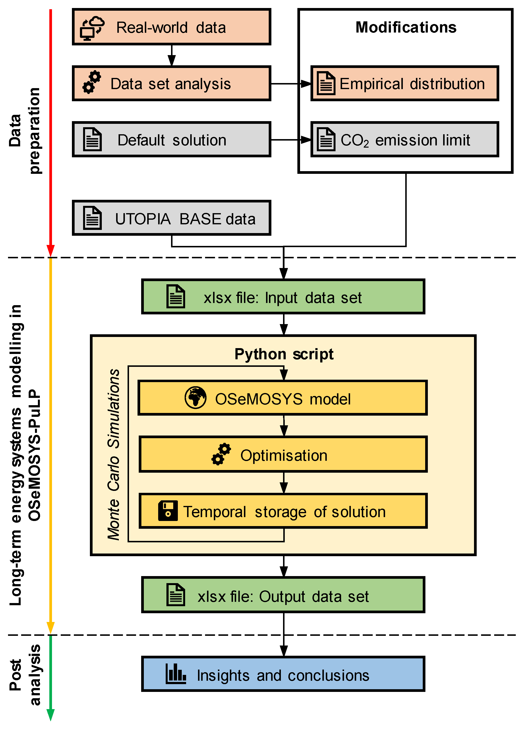
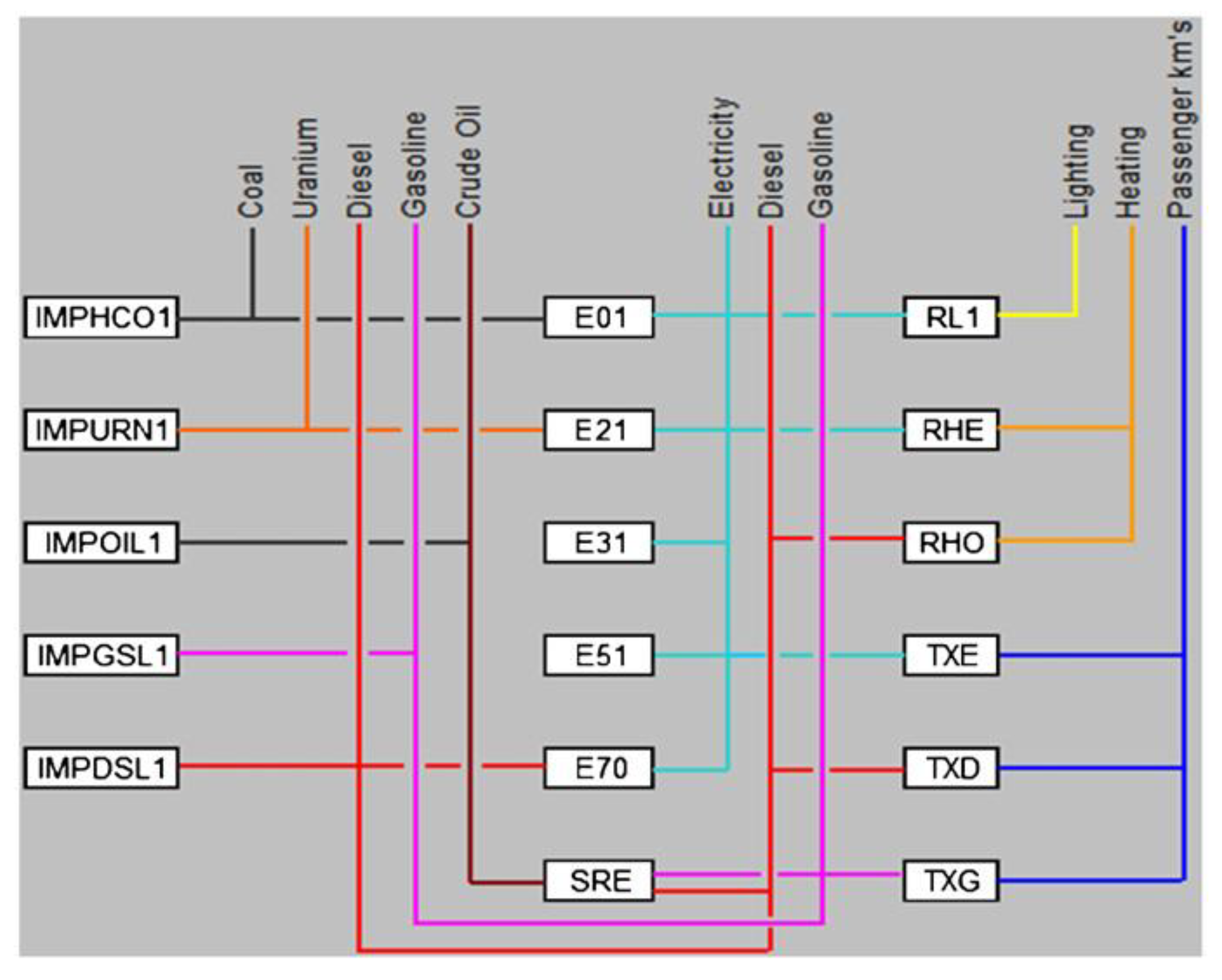
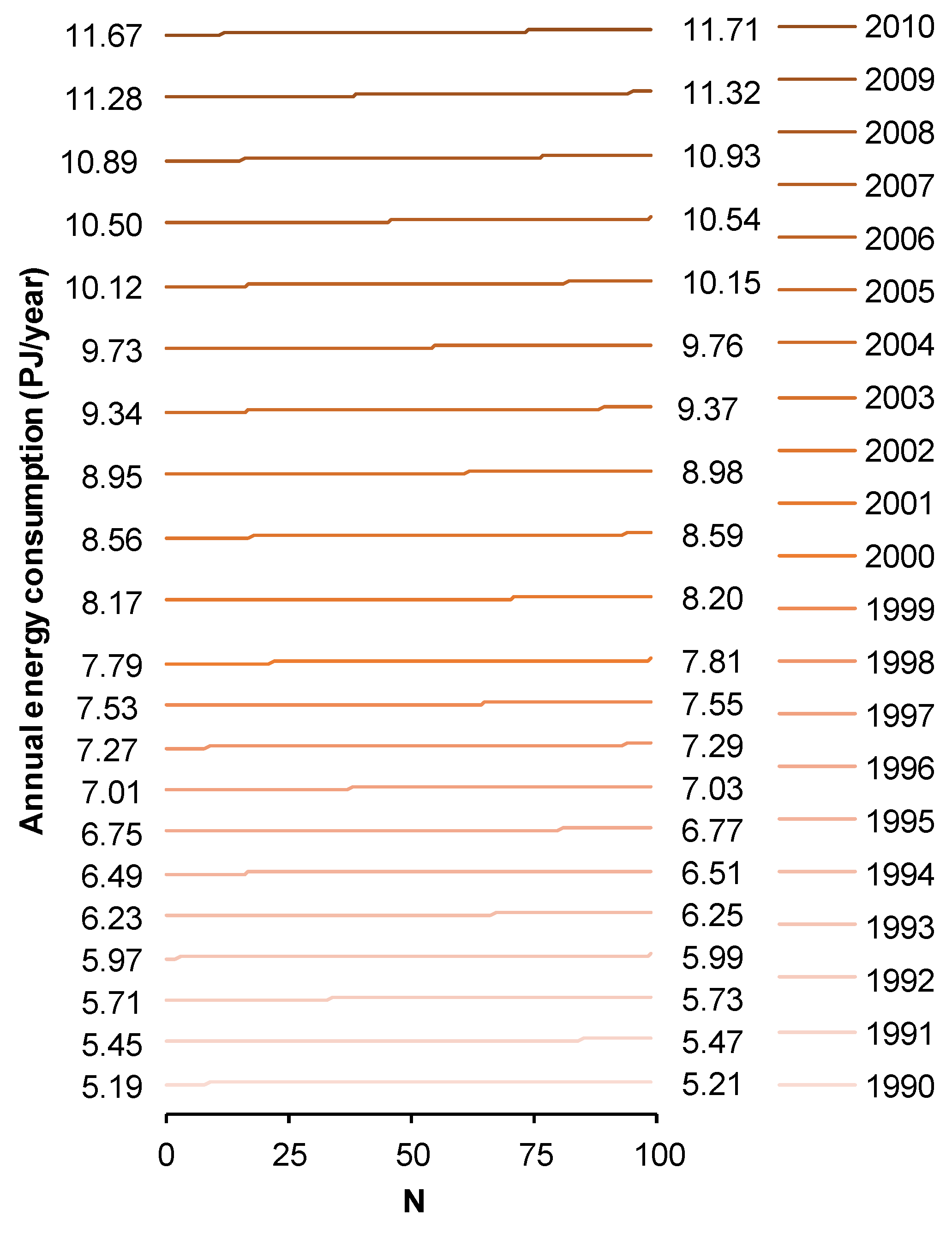
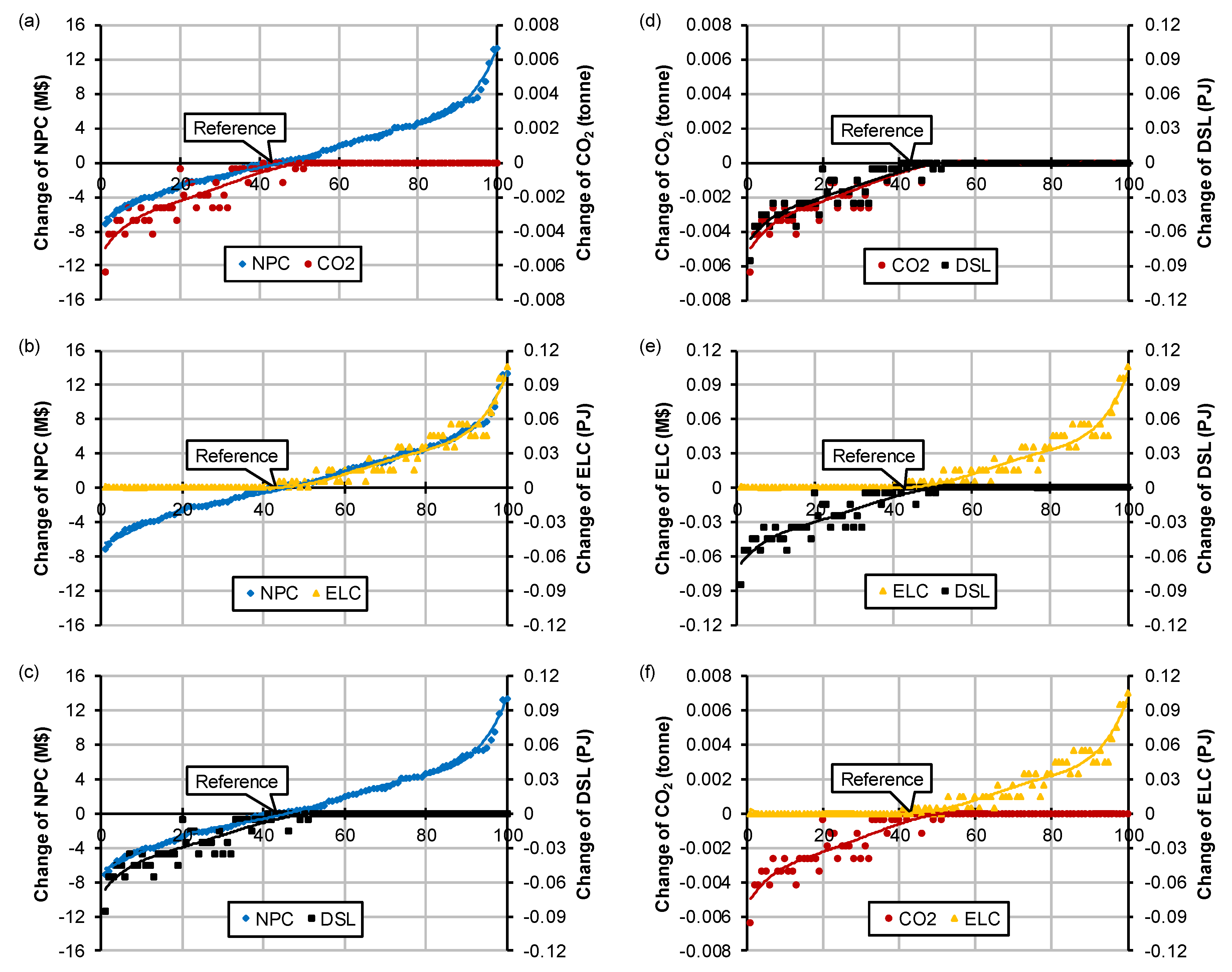
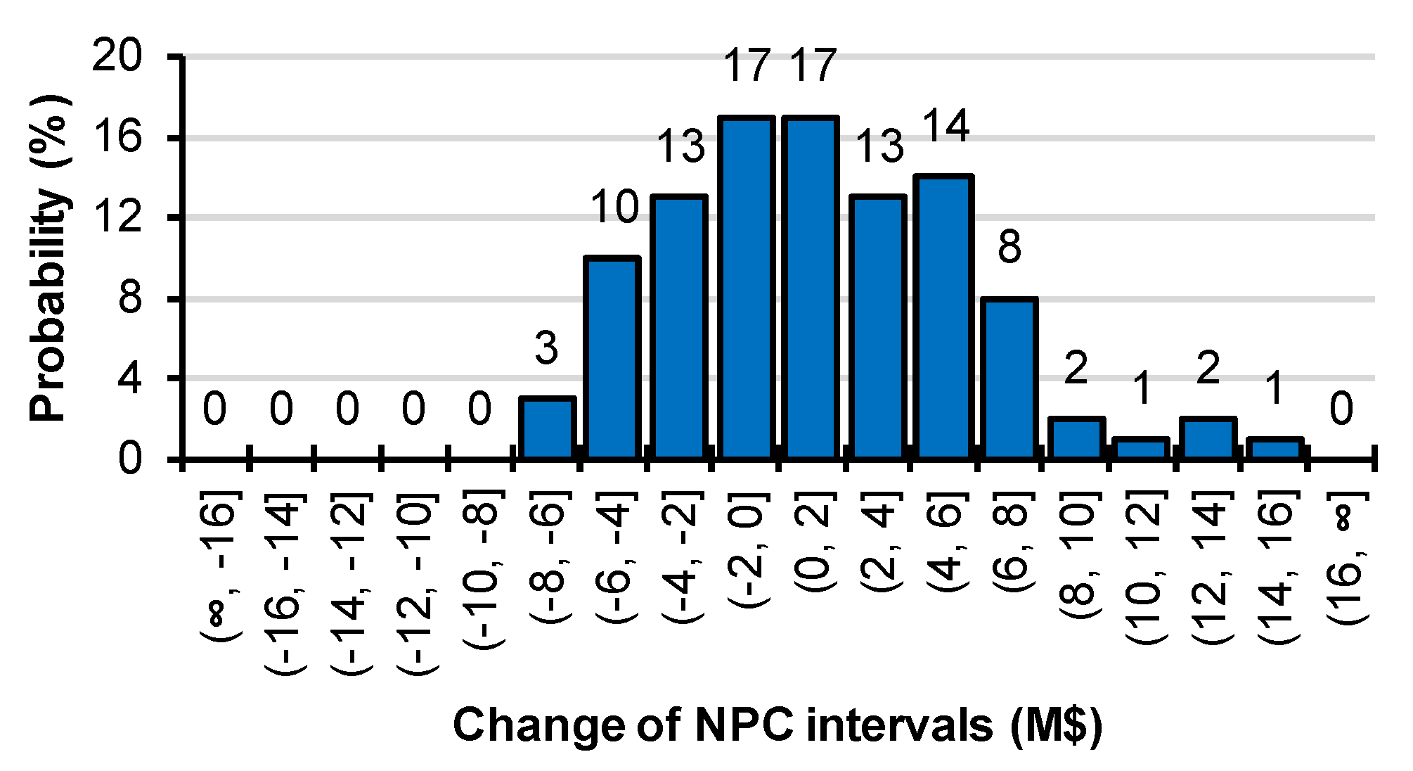
Table 1.
Descriptive statistics of the annual energy consumption values. Unit: TJ/year if not otherwise stated in parentheses.
Table 1.
Descriptive statistics of the annual energy consumption values. Unit: TJ/year if not otherwise stated in parentheses.
| N (-) | Mean | SD | Min. | Q25 | Median Q50 | Q75 | Max. | Skew. (-) | Kurt. (-) |
|---|---|---|---|---|---|---|---|---|---|
| 100 | 1608.62 | 1.31 | 1605.82 | 1607.66 | 1608.60 | 1609.47 | 1611.46 | 0.011 | −0.616 |
© 2019 by the authors. Licensee MDPI, Basel, Switzerland. This article is an open access article distributed under the terms and conditions of the Creative Commons Attribution (CC BY) license (http://creativecommons.org/licenses/by/4.0/).
Share and Cite
MDPI and ACS Style
Dreier, D.; Howells, M. OSeMOSYS-PuLP: A Stochastic Modeling Framework for Long-Term Energy Systems Modeling. Energies 2019, 12, 1382. https://doi.org/10.3390/en12071382
AMA Style
Dreier D, Howells M. OSeMOSYS-PuLP: A Stochastic Modeling Framework for Long-Term Energy Systems Modeling. Energies. 2019; 12(7):1382. https://doi.org/10.3390/en12071382
Chicago/Turabian StyleDreier, Dennis, and Mark Howells. 2019. "OSeMOSYS-PuLP: A Stochastic Modeling Framework for Long-Term Energy Systems Modeling" Energies 12, no. 7: 1382. https://doi.org/10.3390/en12071382
Note that from the first issue of 2016, this journal uses article numbers instead of page numbers. See further details here.