Nature-Inspired MPPT Algorithms for Partially Shaded PV Systems: A Comparative Study

Abstract

PV generating sources are one of the most promising power generation systems in today’s power scenario. The inherent potential barrier that PV possesses with respect to irradiation and temperature is its nonlinear power output characteristics. An intelligent power tracking scheme, e.g., maximum power point tracking (MPPT), is mandatorily employed to increase the power delivery of a PV system. The MPPT schemes experiences severe setbacks when the PV is even shaded partially as PV exhibits multiple power peaks. Therefore, the search mechanism gets deceived and gets stuck with the local maxima. Hence, a rational search mechanism should be developed, which will find the global maxima for a partially shaded PV. The conventional techniques like fractional open circuit voltage (FOCV), hill climbing (HC) method, perturb and observe (P&O), etc., even in their modified versions, are not competent enough to track the global MPP (GMPP). Nature-inspired and bio-inspired MPPT techniques have been proposed by the researchers to optimize the power output of a PV system during partially shaded conditions (PSCs). This paper reviews, compares, and analyzes them. This article renders firsthand information to those in the field of research, who seek interest in the performance enhancement of PV system during inhomogeneous irradiation. Each algorithm has its own advantages and disadvantages in terms of convergence speed, coding complexity, hardware compatibility, stability, etc. Overall, the authors have presented the logic of each global search MPPT algorithms and its comparisons, and also have reviewed the performance enhancement of these techniques when these algorithms are hybridized.

1. Introduction

The increasing load demand on one side and the depletion of fossil fuels on the other side forces the world to look for alternative energy resources. Also, the concern regarding pollution through the greenhouse effect and other environmental issues associated with the conventional energy sources make renewable energy resources (RES) more attractive [1]. Among various non-conventional sources, solar energy is more widely used because of the abundant availability of solar irradiation on the earth’s surface [2]. The photovoltaic (PV) cells convert direct sunlight into electricity, but as the solar irradiance and temperature are fluctuating in nature, as a result, it reduces the PV panel efficiency. The main drawbacks of the PV system are its highly intermittent nature, lower conversion efficiency, lower rating, high implementation cost, and maintenance issues. PV panels also get affected due to partial shading because of clouds, tree branches, birds, etc. These factors make it essential to deploy a dc–dc converter with an MPPT technique for tracking the maximum power point from the PV panel under all operating conditions. The MPPT control algorithm is employed along with the dc–dc converter, where the control algorithm adjusts the duty cycle according to the variation in solar irradiation and temperature, which will boost the lower voltage output of the PV system. A PV cell has very low power rating [3,4,5,6], and these cells can be connected in series or parallel according to the required current and voltage rating. The series and parallel combination constitute a PV module and the modules are connected together to form a PV array [7]. This makes power electronic interfaces indispensable in any PV system for ensuring the system voltage compatible with a load or grid [8]. PV panels can be implemented as a rooftop setup and it can also operate in standalone mode and grid-connected mode [9].

For a PV system, the output voltage depends on the temperature of the panel and the current value of the irradiance level. The PV system gives the optimum output under the standard test condition (STC-irradiance = 1000 W/m², temperature = 25 °C, 1.5 air mass) [3,10]. MPPT trackers embody a control algorithm and converter to ensure that PV panels operate at MPP to render maximum possible power. This tracking scheme becomes futile when PV panels are partially shaded. In the research arena, there was a paradigm shift in MPPT algorithms as a host of research articles are being published every year on global search algorithms [8,9]. Many studies have been done toward developing an efficient and reliable MPPT algorithm to extract the maximum operating power point from the PV panel [11,12,13]. Both conventional and computational intelligence algorithms are used for MPPT [14,15]. Most of the conventional algorithms perform effectively under uniform solar irradiation and temperature but fail to track the true maximum operating point during varying weather or partial shading conditions [16,17].

The efficient nature-inspired algorithms based on MPPT techniques are the particle swarm optimization (P&O) algorithm, ant colony optimization (ACO) algorithm, artificial bee colony (ABC) algorithm, differential evolution (DE), etc. These algorithms are used for global search problems and can operate effectively under uniform solar irradiation and temperature, as well as partial shading and rapidly changing environmental conditions. Hybridization of these algorithms also has been done for enhancing the performance and reliability of these algorithms. In Reference [18], the authors have proposed a swarm chasing MPPT algorithm for module integrated converters and the performance is also compared with conventional P&O method. Here, the swarm-chasing technique is found to be more superior. Comparative study on well-entrenched global peak tracking algorithms is archived in a research forum [15,19]. Some researchers paid due credit to the conventional algorithms and examined whether the algorithms could be sustained during partial shading. In Reference [19], conventional and computational intelligence MPPT techniques were presented, which describes the working of each algorithm with their merits and demerits. The quest toward proposing new algorithms has not dwindled as one can witness recent research articles on global search MPPT [8,9,13,15].

In this paper, a review has been done for five evolutionary algorithms that are reliable and more pragmatic for practical deployment. This paper has been framed in such a manner that it gives a clear understanding of PV characteristics, partial shading, and MPP search mechanisms. The paper is organized in such a way that Section 2 presents PV modeling and PV characteristics analysis during both uniform irradiation condition and PSCs. Section 3 discusses the soft computing algorithms reviewed in this paper, whereas Section 4 follows a brief discussion about the reviewed algorithms. The concluding part is given in Section 5.

2. PV Modeling and Its Characteristic Curves

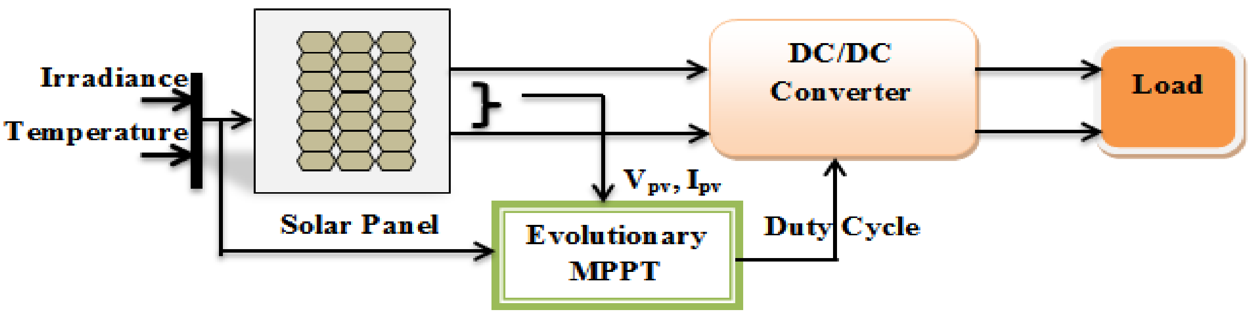
Figure 1 depicts a general block diagram of a PV generating system. In the given diagram, a PV panel connected with a dc–dc converter and the duty cycle of the converter is controlled by the MPPT algorithm. The MPPT algorithm will sense the required parameters from the solar system, and accordingly, it modifies the converter duty cycle. Hence, under all conditions, maximum output power is obtained from the panel. Then the converter output can be directly connected to the dc load or it can also be given to ac loads by connecting them through an inverter.

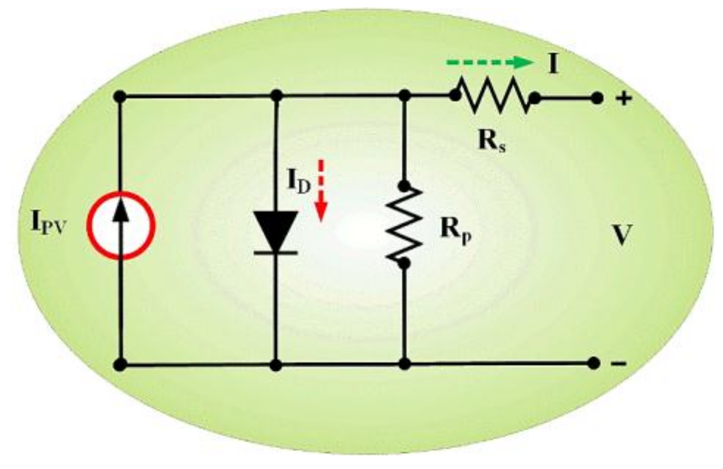
A PV module consists of many solar cells that are generally made up of silicon material. When the light energy falls on the solar cell, then the electrons start to move and current flows. Solar cells are considered current sources. There are many types of solar cell models, among which, the single diode model is well established and a simple structure [10,20]. In this paper, a single diode model solar cell is shown in Figure 2. It is basically a diode connected in parallel with a current source along with one shunt and one series resistor. In the figure, I_pv is the current generated by light, I_D is the current across diode, whereas I_sh represents the current flowing through a shunt resistance R_sh, and I is the output current. For the mathematical modeling of the PV system, the basic equations are given below.

$$\mathrm{I}={\mathrm{I}}_{\mathrm{PV}}-{\mathrm{I}}_{\mathrm{o}}\left[\exp \left(\frac{\mathrm{V}+{\mathrm{IR}}_{\mathrm{s}}}{{\mathrm{aV}}_{\mathrm{T}}}\right)-1\right]-\frac{\mathrm{V}+{\mathrm{IR}}_{\mathrm{s}}}{{\mathrm{R}}_{\mathrm{sh}}}$$

(1)

where V_T is the PV array thermal voltage = kT/q. I_P represents the photocurrent, I_o represents reverse saturation current, and R_s and R_sh represent the series and shunt resistance respectively, a is the diode ideality factor, q is the charge of the electron i.e., 1.6 × 10⁻¹⁹ C, k represents Boltzmann’s constant (1.3806503 × 10⁻²³ J/K), and T is the temperature.

$${\mathrm{I}}_{\mathrm{o}}={\mathrm{I}}_{\mathrm{o}\_\mathrm{STC}}{\left[\frac{{\mathrm{T}}_{\mathrm{STC}}}{\mathrm{T}}\right]}^3\exp \left[\frac{{\mathrm{qE}}_{\mathrm{g}}}{\mathrm{ak}}\left(\frac{1}{{\mathrm{T}}_{\mathrm{STC}}}-\frac{1}{\mathrm{T}}\right)\right]$$

(2)

In the above equation E_g represents band gap energy of the semi-conductor material and I_{o_STC} denotes the nominal saturation current at STC, T_STC is the temperature under STC (25 °C).

In simplified form, I_o can be written as

$${\mathrm{I}}_{\mathrm{o}}=\frac{\left({\mathrm{I}}_{\mathrm{sc},\mathrm{STC}}+{\mathrm{K}}_{\mathrm{I}}\Delta \mathrm{T}\right)}{\exp \left[\left({\mathrm{V}}_{\mathrm{oc},\mathrm{STC}}+{\mathrm{K}}_{\mathrm{v}}\Delta \mathrm{T}\right)/{\mathrm{aV}}_{\mathrm{T}}\right]-1}$$

(3)

here K_i is the coefficient of the short circuit current, K_v is the open circuit voltage coefficient, I_{sc_STC} is the short circuit current under STC, V_{oc_STC} is the open circuit voltage under STC, and ΔT = T − T_STC.

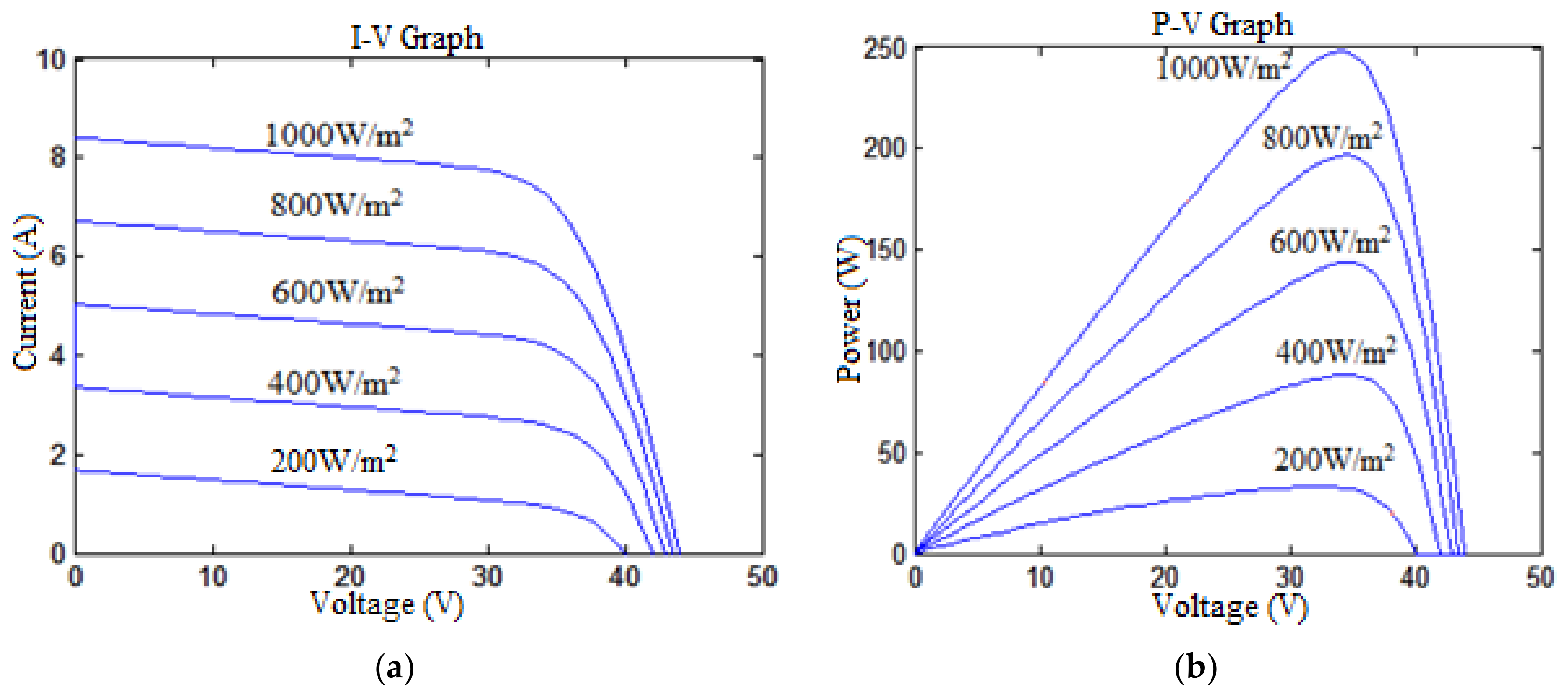
In Figure 3a,b the I–V graph and P–V graph for different irradiation levels are shown. The I–V graph shown in Figure 3a shows that according to the temperature and irradiance, the voltage and current value also varies. Here, the current value depends on the irradiance, i.e., directly proportional, and the voltage depends on the temperature [20]. Hence, the PV operating point does not stay at the maximum operating value and it varies with the environmental conditions, which in turn, reduces the power. Therefore, it is preferable to install more PGS than the required demand, but simultaneously, it increases the cost [21]. Therefore, the dc–dc converter with an effective MPPT technique is deployed for the PV systems to modify the converter duty cycle according to the environmental conditions and thereby tracks the maximum power point for all operating conditions. During uniform irradiance, the P–V graph shows only one peak power point, which gives the corresponding maximum voltage and current. Hence, the conventional MPPT techniques would suffice to track the true MPP and is found to be reliable.

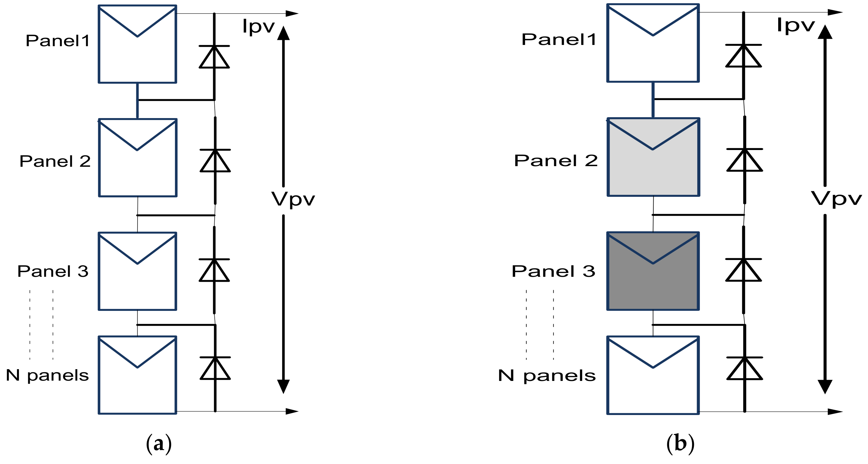
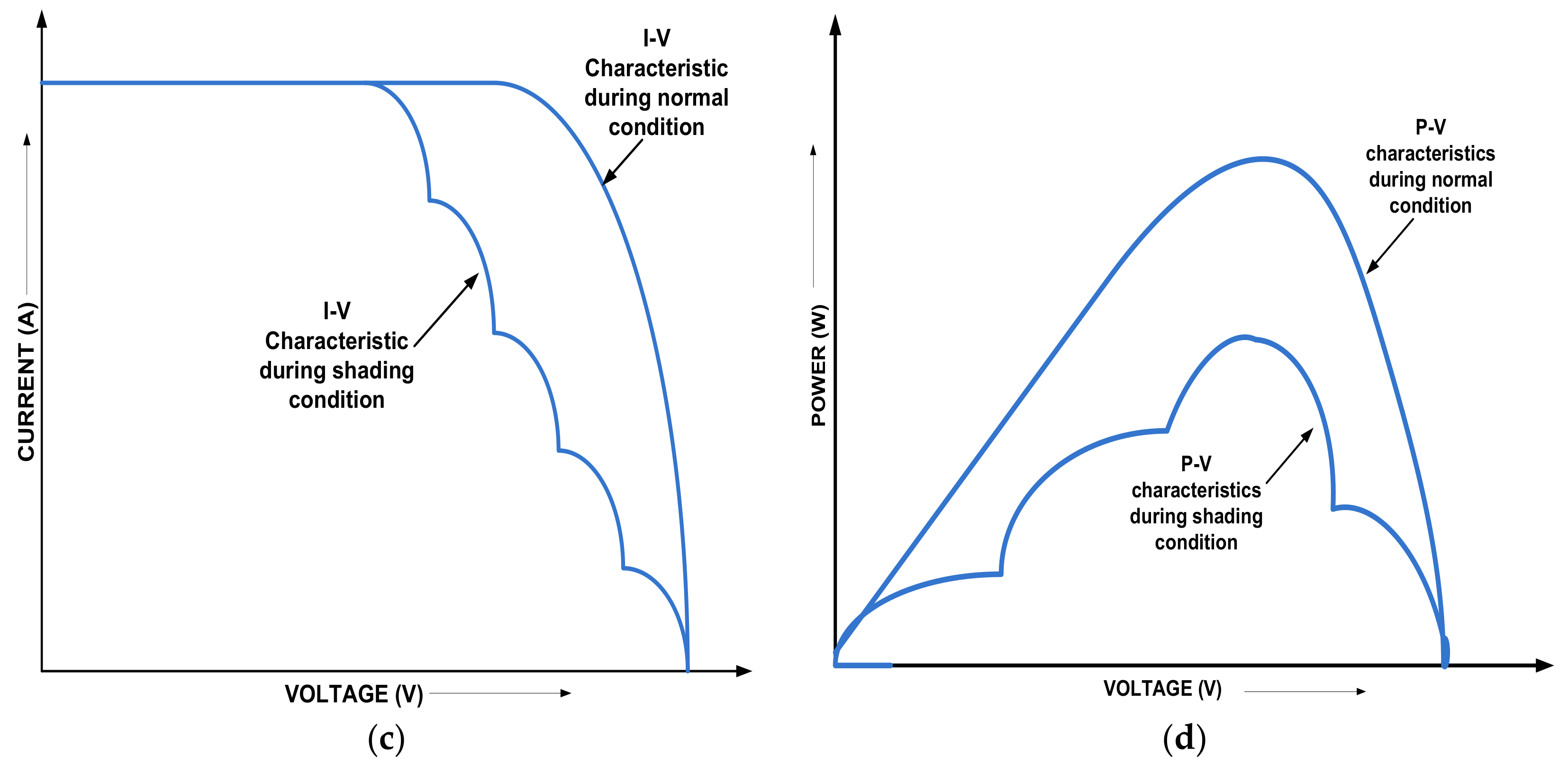
However, when some of the PV panels in an array receive non-uniform irradiation and temperature, i.e., they are shaded, then the power production of the shaded panel decreases relative to an unshaded one. The shaded panels absorb a large amount of current from the unshaded panels in order to operate. This condition is called hot spot formation and this damages the PV panel [22,23]. To avoid this condition, a bypass diode is connected in parallel across each panel, as shown in Figure 4a,b, which provides another way for conduction during the occurrence of partial shading [24]. As shown in Figure 4c,d, during the partial shading condition, there exist multiple peak points in the P–V characteristics graph, among which only one point is the true maximum power point. These multiple peak points are considered the local maximum power points (LMPPs), and among all the LMPPs, the true MPP is called the global maximum power point (GMPP). Most of the conventional MPPT techniques fail to identify the GMPP among all the LMPP. For this purpose, many researchers have proposed various stochastic, evolutionary, and swarm-based algorithms and hybridization of these algorithms has also been done for more reliable and effective MPP tracking.

3. Intelligent Nature Inspired Algorithms: An Overview

The specific evolutionary algorithms discussed are

• particle swarm optimization (PSO) algorithm
• differential evolution (DE) algorithm
• ant colony optimization (ACO) algorithm
• artificial bee colony (ABC) optimization algorithm
• bacteria foraging optimization algorithm (BFOA).

The analysis of these algorithms has been done with respect to the convergence speed, execution, and reliability.

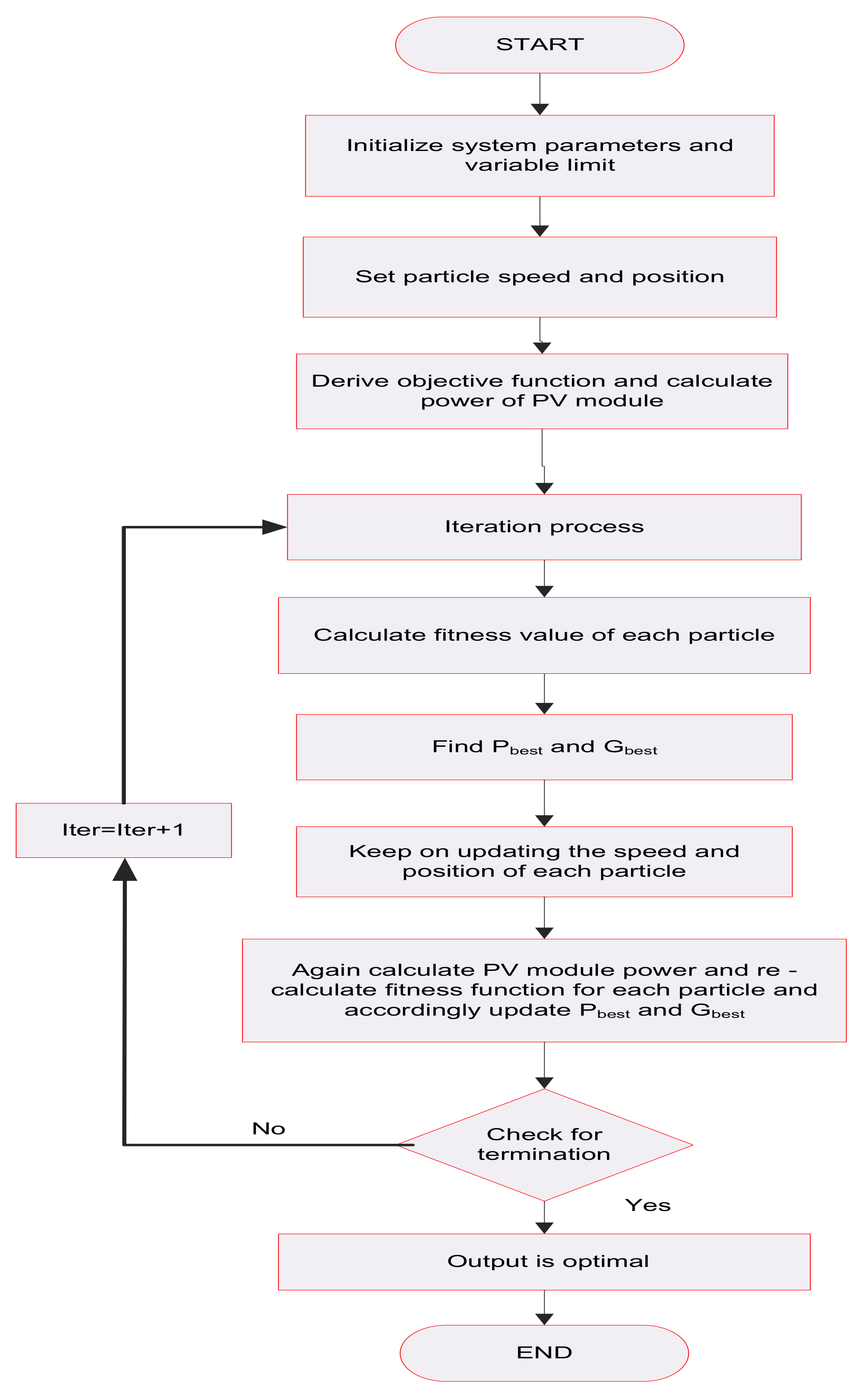
3.1. Particle Swarm Optimization (PSO)

PSO is the most widely used algorithm used for the MPPT technique. This algorithm was discovered in 1995 by Ebehart and Kennedy. PSO is widely accepted by researchers due to its simple and easy to implementation characteristics. This algorithm is motivated by the communal activity of the crowding of birds and schooling activity of fish. PSO is a global optimization algorithm that finds the best solution in a multi-dimensional path. Therefore, it is able to track the GMPP from all local MPPs even when the PV panel is under a partial shading condition or the PV panel possesses multiple peak points. PSO uses many operating agents that share information about their respective search behavior, where all agents are termed as a particle. Here, a number of particles move in the search space in order to get the best solution. Each particle adjusts its movement by following the best solution and mean while searches for new solutions will be in progress [25]. The particle referred here can be voltage or duty cycle. For finding the optimal solution, the particle must follow the best position of its own or the best position of its neighbor. The mathematical representation of the PSO algorithm is given in the following equations [26,27]:

$${\mathrm{u}}_{\mathrm{i}}\left(\mathrm{k}+1\right)={\mathrm{qu}}_{\mathrm{i}}\left(\mathrm{k}\right)+{\mathrm{c}}_1{\mathrm{r}}_1\left({\mathrm{p}}_{\mathrm{best},\mathrm{i}}-{\mathrm{g}}_{\mathrm{i}}\left(\mathrm{k}\right)\right)+{\mathrm{c}}_2{\mathrm{r}}_2\left({\mathrm{g}}_{\mathrm{best},\mathrm{i}}-{\mathrm{g}}_{\mathrm{i}}\left(\mathrm{k}\right)\right)$$

(4)

$${\mathrm{g}}_{\mathrm{i}}\left(\mathrm{k}+1\right)={\mathrm{g}}_{\mathrm{i}}\left(\mathrm{k}\right)+{\mathrm{u}}_{\mathrm{i}}\left(\mathrm{k}+1\right)$$

(5)

where i = 1, 2, 3,..., N.

u_i—velocity of the particle

g_i—particle position

k—number of iterations

q—inertia weight

r₁,r₂—random variables which are distributed uniformly between [0,1]

c₁,c₂—cognitive and social co-efficient respectively

p_best—individual particle’s best position

g_best—best position between all the particle’s individual best position

PSO finds the global maxima voltage point according to the maximum power in the P–V graph. For this, we need to specify PSO parameters such as power and voltage value, size of the swarm, and number of iterations. PSO stores the best value as p_best and continues to update until it finds the g_best point or it satisfies the objective function [15,27,28]:

$${\mathrm{p}}_{\mathrm{best},\mathrm{i}}={\mathrm{g}}_{\mathrm{i}}\left(\mathrm{k}\right)$$

(6)

$$\mathrm{f}({\mathrm{g}}_{\mathrm{i}}\left(\mathrm{k}\right))>\mathrm{f}({\mathrm{g}}_{\mathrm{i}}\left(\mathrm{k}+1\right))$$

(7)

where the function “f” is the PV panel operating power. During partial shading, the particles are re-initialized to find g_best and it must satisfy the below condition. A flowchart of the PSO algorithm is given in Figure 5.

$$\left|\frac{\mathrm{P}({\mathrm{g}}_{\mathrm{i}+1})-\mathrm{P}({\mathrm{g}}_{\mathrm{i}})}{\mathrm{P}({\mathrm{g}}_{\mathrm{i}})}\right|>\Delta \mathrm{P}$$

(8)

In Reference [24], a cost-effective PSO algorithm is presented, which uses one single pair of sensors for controlling multiple PV arrays. The algorithm is also compared with many conventional techniques, from which, the proposed algorithm is found to be more effective and it also tracks the MPP even during partial shading conditions. The authors in Reference [9] have presented a PSO algorithm integrated with an overall distribution (OD) algorithm. The OD technique is used to efficiently track the MPP during any shading conditions and is again integrated with PSO to improve the accuracy of the MPPT technique. A novel two-stage PSO MPPT is proposed in Reference [29]. Here, for partial shading conditions and to achieve improved convergence speed, a shuffled frog leaf algorithm (SFLA) with an adaptive speed factor is implemented with PSO. For partially shaded PV power systems, a modified PSO is presented in Reference [30] whose effectiveness is shown in the paper. Many studies have been done using PSO as an MPPT technique for both uniform irradiation and partially shaded conditions. However, the standard PSO performance is enhanced and modified by using hybridization and modification in the algorithm [25,28,31,32,33,34,35], which increases the system efficiency and is found to be more reliable.

3.2. Differential Evolution (DE)

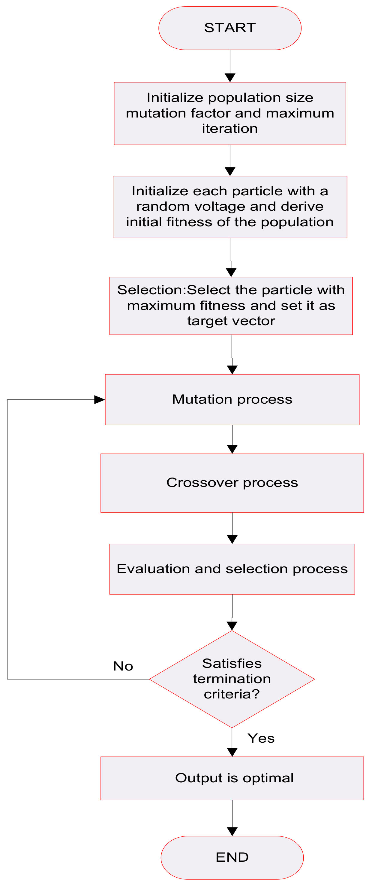
This algorithm was suggested by Price and Storn in 1995. DE is a randomly varying population-based algorithm and it finds its application in global optimization problems [36]. This algorithm is well-suited for non-linear, non-differentiable, multi-dimensional problems [37]. Therefore, this algorithm can be implemented for PV panel maximum power extraction as the PV characteristics possesses a highly non-linear graph as they are intermittent in nature [16,20]. Furthermore, even during partial shading conditions, it can track the global optimum power point [38,39]. In the DE algorithm, the complexity reduces as it requires much fewer parameters (particles) to tune. This tuning of particles makes sure that in every iteration, the particles converge toward the best solution in the search space. DE algorithm follows various steps for optimization and those are initialization, mutation, recombination/crossover, and selection [40]. The DE algorithm flowchart is shown in Figure 6.

3.2.1. Initialization

DE optimizes the problem by using different formulas for creating new particles and also by maintaining the population size at the same time. In the search space, out of the existing particles and newly updated particles, the best fitness value particles only remain and others having the least fitness value are replaced. In DE optimization, various control processes are carried out step by step as discussed below. For optimization using DE, at first, initial parameters, population, and number of generations must be initialized [37,41,42].

If a function with “P” real parameters must be optimized, then the population size is taken as “N”, where the “N” value should not be less than 4.

Hence, the parameter vectors can be written as:

$${\mathrm{x}}_{\mathrm{i},\mathrm{G}}=[{\mathrm{x}}_{1,\mathrm{i},\mathrm{G}},{\mathrm{x}}_{2,\mathrm{i},\mathrm{G}},{\mathrm{x}}_{3,\mathrm{i},\mathrm{G}},\dots \dots ,{\mathrm{x}}_{\mathrm{P},\mathrm{i},\mathrm{G}}]$$

(9)

In the above equation i = 1, 2, …, N; and G is the number of generations.

During initialization process, the user sets a predefined upper and lower boundary value for each particle:

$${\mathrm{x}}_{\mathrm{j}}^{\mathrm{L}}\le {\mathrm{x}}_{\mathrm{j},\mathrm{i},1}\le {\mathrm{x}}_{\mathrm{j}}^{\mathrm{U}}$$

(10)

The initial values are chosen randomly for each particle but in uniform intervals between the upper and lower interval of the particle.

3.2.2. Mutation

Here, each individual becomes a target vector. Mutation is performed for all N particles in the search space and hence it expands the search space. For a particular particle ${\mathrm{x}}_{\mathrm{i},\mathrm{G}}$, three random vectors are taken such as ${\mathrm{x}}_{\mathrm{r}1,\mathrm{G}},{\mathrm{x}}_{\mathrm{r}2,\mathrm{G}},{\mathrm{and}\mathrm{x}}_{\mathrm{r}3,\mathrm{G}}$ in such a manner that all the indices i, r1, r2, and r3 are distinct from each other.

For finding out the donor vector (the new particle formed from the mutation process), add the weighted difference of two vectors with the third vector:

$${\mathrm{u}}_{\mathrm{i},\mathrm{G}+1}={\mathrm{x}}_{\mathrm{r}1,\mathrm{G}}+\mathrm{F}\left({\mathrm{x}}_{\mathrm{r}2,\mathrm{G}}-{\mathrm{x}}_{\mathrm{r}3,\mathrm{G}}\right)$$

(11)

where F is the mutation factor, which lies between [0,2]; ${\mathrm{u}}_{\mathrm{i},\mathrm{G}+1}$ is the donor vector.

3.2.3. Crossover

Here, the next generation is formed from the parent particles. Therefore, recombination is performed between the target and mutant vector to get the next generation vector, which is a trial vector. In other words, the trial vector ${\mathrm{u}}_{\mathrm{i},\mathrm{G}+1}$ is formed by considering the elements of the target vector ${\mathrm{x}}_{\mathrm{i},\mathrm{G}}$ and also from the elements of the mutant vector/donor vector ${\mathrm{u}}_{\mathrm{i},\mathrm{G}+1}$.

Crossover may be reached on the D variables when an arbitrarily chosen number between 0 to 1 lies in the range of the CR value, where CR is a constant value and is used for controlling DE parameters. The condition is given as:

$${\mathrm{u}}_{\mathrm{j},\mathrm{i},\mathrm{G}+1}=\left\{\begin{array}{c}{\mathrm{u}}_{\mathrm{j},\mathrm{i},\mathrm{G}+1}\hspace{1em}\hspace{1em}\mathrm{if}\hspace{1em}{\mathrm{rand}}_{\mathrm{j},\mathrm{i}}\le \mathrm{CR} \mathrm{and} \mathrm{j}={\mathrm{I}}_{\mathrm{rand}}\\ {\mathrm{x}}_{\mathrm{j},\mathrm{i},\mathrm{G}}\hspace{1em}\hspace{1em}\mathrm{if}\hspace{1em}{\mathrm{rand}}_{\mathrm{j},\mathrm{i}}>\mathrm{CR} \mathrm{and} \mathrm{j}\ne {\mathrm{I}}_{\mathrm{rand}}\end{array}\right.$$

(12)

where

i = 1, 2, …, N

j = 1, 2, …., D

${\mathrm{rand}}_{\mathrm{j},\mathrm{i}}$ is any value randomly chosen within [0,1]

${\mathrm{I}}_{\mathrm{rand}}$ is a random integer whose value lies within (1, 2, …, D). This value makes sure that ${\mathrm{u}}_{\mathrm{i},\mathrm{G}+1}\ne {\mathrm{x}}_{\mathrm{i},\mathrm{G}}.$

3.2.4. Selection

In DE optimization, the population size is kept constant throughout the generation process. Therefore, a selection criterion provides the best parameter for the next generation. In this process, both parent vector/target vector and the trial vector are compared, and if the trial vector is able to give a better fitness value compared to that of the target vector, then the target vector, i.e., the parent vector, is replaced by the trial vector and the generation gets updated.

DE has its wide acceptance in global search problems. The authors in reference [38] have proposed a DE-based MPPT technique that works with the boost converter for a partially shaded PV system. In the above work, performance of DE algorithm is compared with a conventional algorithm and its efficiency is verified. A detail survey about DE algorithm use in various fields with its advantages and disadvantages is given in reference [43]. The fundamentals of DE, its application to various multi-objective optimization problems, such as constrained, uncertain optimization problems are reviewed in reference [44]. A modified DE with a mutation process being modified, i.e., instead of choosing the parents randomly for mutation, each individual is assigned with a probability of selection, which is inversely proportional to the distance from the mutated individual, is presented in Reference [45]. This modified DE can be applied for solving various optimization problems with some small changes according to the requirement of the optimization problem. A modified DE algorithm for finding the PV model parameters during varying weather conditions and partial shading is given in Reference [46], and the algorithm presented here uses only the PV datasheet information. The original DE and the modified one, and also hybridization of the DE algorithm with various computational techniques or with conventional methods, have been proposed by many researchers [47,48]. The DE algorithm possesses many advantages, but PSO is superior to it in many aspects, such as less coding complexity and parameter tuning.

3.3. Ant Colony Optimization (ACO)

This technique was first proposed by Colorni, Dorigo, and Maniezzo [49]. This is a probability-based algorithm used for a computational problem-solving purpose. This algorithm is inspired by real ants’ behavior for searching the shortest path from their colony to an available food source. The ants will follow the shortest distance between their nest and food [15]. Initially, when the ants search for food, they leave a pheromone trail for other ants to follow the same path. This pheromone trail is a chemical material to which members of the same species respond [50]. The thickness of the pheromone trail increases when it is followed by more ants. These ants may also follow the same path while returning to their nest, thereby making the pheromone trail thicker. Hence, the same path is followed by most of the ants till they find any other shortest path by exchanging information about the pheromone. If the path for the food is not the shortest one, then eventually the pheromone disappears [15,27,51].

ACO in MPPT

For implementing ACO in MPPT, most of the ants’ behavior is considered. Here, ants are initialized first and the objective function is set by considering the irradiation and temperature exposure of each panel. The procedure followed in the ACO algorithm for optimization is given below [50]:

Step 1: Initialize all ants and evaluate K random solutions.

Step 2: Rank solutions according to their fitness value.

Step 3: Perform a new solution.

Step 4: Observe the ant that has the global best position (solution).

Step 5: Upgrade the pheromone trail.

Step 6: Check for termination criteria.

Step 7: If satisfied, then the existing solution is the global best value, else go to Step 3.

Step 8: End.

For finding the pheromone concentration, the formula is given as:

$${\mathrm{T}}_{\mathrm{ij}}={\mathsf{\rho }\mathrm{T}}_{\mathrm{ij}}\left(\mathrm{t}-1\right)+\Delta {\mathrm{T}}_{\mathrm{ij}}$$

(13)

In the above equation

t = 1, 2, 3, …, T

${\mathrm{T}}_{\mathrm{ij}}$ is the revised concentration of the pheromone

$\Delta {\mathrm{T}}_{\mathrm{ij}}$ is the change in pheromone concentration

ρ is the pheromone concentration rate.

The main function of ACO is to track the global peak power operating point at which the PV system operates.

Fitness function = Panel 1(V₁ × (I(S₁,T₁))) + Panel 2(V₂ × (I(S₂,T₂))) + Panel 3(V₃ × (I(S₃,T₃))) +…+ Panel N(V_N × (I(S_N,T_N)))

(14)

where V₁, S₁, and T₁ represent the panel 1 voltage, irradiance, and temperature, respectively, and so on for the other panels.

In references [42,52], the authors have used an ACO algorithm to improve the PV system efficiency for a partial shading condition. Apart from the MPPT techniques, the ACO has wide application such as optimization in hydro-electric generation scheduling, optimal reactive power dispatch for line loss reduction, microwave corrugated filter design, etc. [53,54,55]. For further improving the ACO performance, i.e., its convergence speed and ease of operation, it can also be combined with various evolutionary and conventional algorithms. The ACO algorithm performs excellently for partially shaded PV modules with improved system performance [56,57]. In reference [58], an ACO-PSO-based MPPT technique is given for a partially shaded PV system. The proposed hybrid algorithm is implemented with an inter-leaved boost converter, which improves the output power and provides a constant voltage to the load. The authors in reference [59] have proposed a hybrid algorithm by considering the simplest conventional and widely used P&O (perturb and observe) with ACO. P&O fails during partial shading and falls on local MPP, hence in the hybrid algorithm, ACO helps the algorithm converge towards the GMPP. This hybrid algorithm improves the system performance and reliability.

3.4. Artificial Bee Colony (ABC)

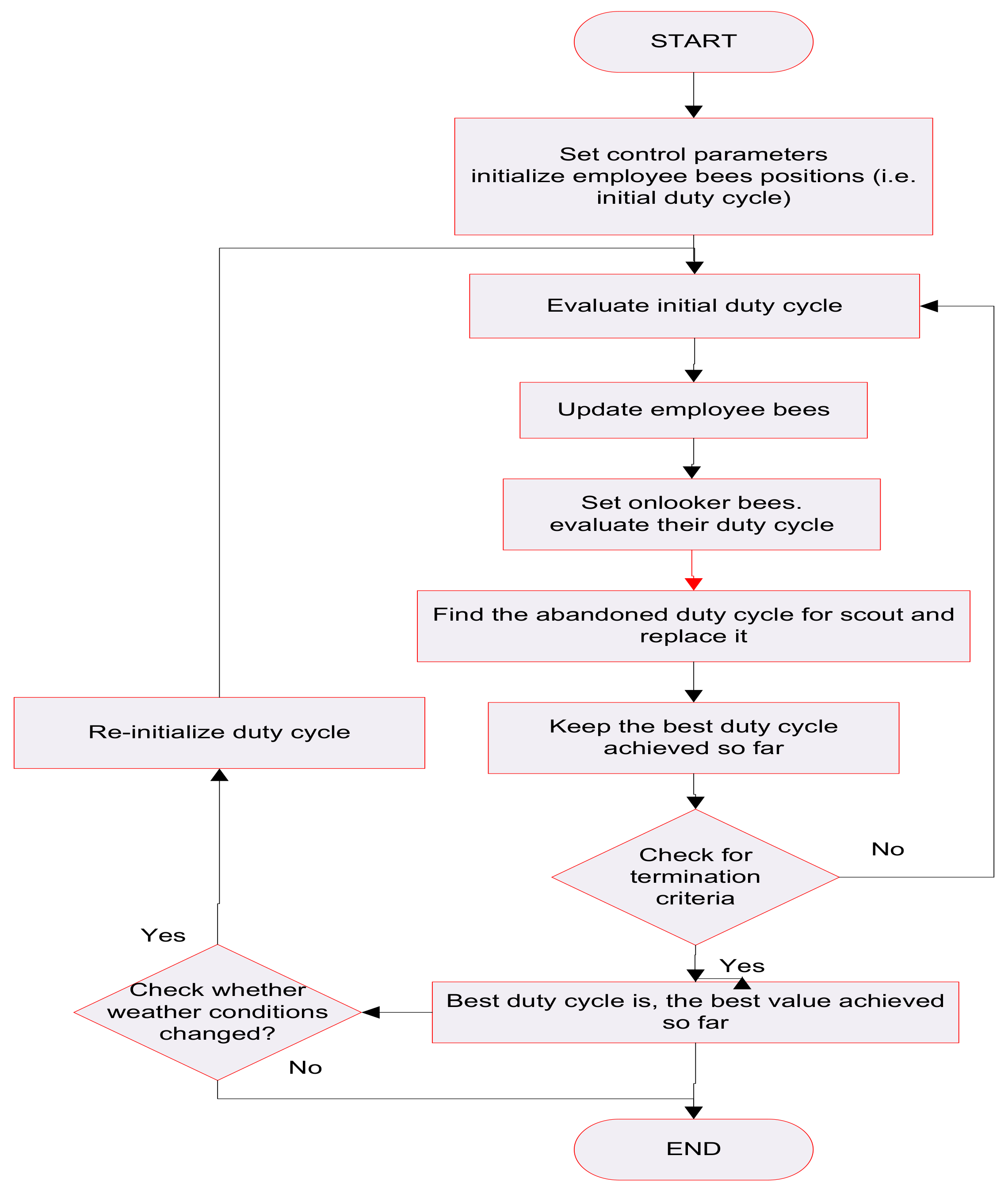
This swarm technology-based meta-heuristic algorithm is used to solve multi-dimensional and multi-modal problems. The algorithm was proposed by Karaboga [60]. It is inspired by various behaviors of honeybees such as foraging, learning, memorizing, and sharing of information for optimization [61,62,63]. For the ABC algorithm, food locations are considered as effective solutions and the amount of nectar it produces defines the quality of the food source (i.e., fitness of the food source) [64]. Here, the bees are classified into three categories (first one is called employed bees, second one is onlooker bees, and the third one is scout bees), and the three types of bees perform mostly three types of foraging behavior, which are first searching the food source, then employing the employed bees for getting the food from the food source, and lastly, discarding the food source due to its lack of nectar quality [15,27]. The employed bees search for food or find the food location. The bee that makes decision regarding the food source is called the onlooker bee. The food sources discovered by the employed bees that cannot be improved are discarded, and the employed bees that found them become scout bees. Here, the number of bees is equal to the number of employed scout bees and onlooker bees. Flowchart of ABC algorithm is given in Figure 7.

ABC as the MPPT

For analyzing the MPPT technique based on the ABC algorithm, every candidate solution is considered as duty cycle “d” of the dc–dc converter. Hence, here the optimization function has only one parameter “d” to be optimized. Let us consider a D-dimensional problem having N_P food sources has to be optimized, where N_P is the number of number of bees in the search space. Hence, by assuming that each food source has one employed bee, then the ith food source location for the tth iteration is given by

$${\mathrm{X}}_{\mathrm{i}}^{\mathrm{t}}={\left[{\mathrm{x}}_{\mathrm{i}1}^{\mathrm{t}},{\mathrm{x}}_{\mathrm{i}2}^{\mathrm{t}},{\mathrm{x}}_{\mathrm{i}3}^{\mathrm{t}},\dots {\mathrm{x}}_{\mathrm{id}}^{\mathrm{t}},\dots {\mathrm{x}}_{\mathrm{iD}}^{\mathrm{t}}\right]}^{\mathrm{T}}$$

(15)

Randomly generate the food source as:

$${\mathrm{x}}_{\mathrm{id}}={\mathrm{L}}_{\mathrm{d}}+\mathrm{r}\left({\mathrm{U}}_{\mathrm{d}}-{\mathrm{L}}_{\mathrm{d}}\right)$$

(16)

where ${\mathrm{U}}_{\mathrm{d}}$ and ${\mathrm{L}}_{\mathrm{d}}$ are upper and lower limit for the dth dimension problem, and r is a random number whose value is chosen between [0,1].

In the next step, the employed bees search for a new food source V_i near to X_i along with a randomly selected dimension d:

$${\mathrm{v}}_{\mathrm{id}}={\mathrm{x}}_{\mathrm{id}}+\mathsf{\beta }\left({\mathrm{x}}_{\mathrm{id}}-{\mathrm{x}}_{\mathrm{jd}}\right)$$

(17)

where ${\mathrm{v}}_{\mathrm{id}}$ is the new food source; j is a randomly chosen vector where $\mathrm{i}\ne \mathrm{j}\in \left(1,2,3,\dots {\mathrm{N}}_{\mathrm{P}}\right)$ and β is a randomly chosen value between [1,−1].

In the above condition, if it is found that the new food source is better than that of the old one, then the new food source gets updated, whereas the old one is discarded; else, the old food source remains in the next iteration [15].

Again, the available food source information is shared with onlooker bees and the food source is selected by the onlooker bees based on a probability criteria:

$${\mathrm{P}}_{\mathrm{i}}=\frac{{\mathrm{fitness}}_{\mathrm{i}}}{{{\displaystyle \sum }}_{\mathrm{n}=1}^{{\mathrm{N}}_{\mathrm{P}}}{\mathrm{fitness}}_{\mathrm{n}}}$$

(18)

In this step, the employed bees also get updated with the help of a greedy selection process. In the next step, after the prescribed number of iterations or when the limit values for the new food source quality have not improved, then the food source gets abandoned and goes for termination. The bees associated with the abandoned food sources become scout bees and search for new available food sources and checks for termination criteria. If the available solutions are acceptable and maximum iterations are reached, then the process terminates; otherwise, it continues the search.

The performance analysis of the ABC algorithm is given in reference [65]. Here, the performance of the algorithm is compared with PSO, DE, and other evolutionary algorithms for multi-modal and multi-functional problems where ABC is found to be giving better result compared to others. ABC has successfully been implemented for leaf-constrained minimum spanning problems too [66]. In reference [67], the authors have done a comparative study of the ABC algorithm for a large set of numerical optimization problems and the results obtained are compared with population-based algorithms. It was found that the results obtained by ABC are superior, and in some cases, same as the population-based algorithms where ABC has the advantage of having less control parameters than others. ABC-based MPPT techniques for PV system are given in Reference [68] and the results are compared with the P&O algorithm where the ABC-based MPPT gives a better performance. From various researchers, the effectiveness of the ABC algorithm as an MPPT technique for both uniform and partial shading conditions are shown and found to be better than the existing techniques [69,70,71]. A modified ABC algorithm (MABC) is presented in reference [72] whose performance is compared with the genetic algorithm (GA), PSO, and ABC, and was found to be more suitable for reducing the power loss of PV modules during a partial shading condition.

3.5. Bacteria Foraging Optimization Algorithm (BFOA)

This is a nature-inspired algorithm that is inspired by various foraging behaviors of Escherichia Coli (E. Coli). The E. Coli bacteria present inside the intestine of humans and animals possesses various multi-functional foraging behaviors so as to maximize the consumption of energy per unit time for one particular foraging process. When the foraging process occurs due to the environmental conditions, the bacterium with a high fitness value or those that are able to withstand the environmental changes continue to survive and the others get eliminated [73]. These bacteria follows four basic steps for getting to a nutrient-rich location, i.e., for foraging. These four steps are chemotaxis, swarming, reproduction, and elimination-dispersal [74].

3.5.1. Chemotaxis

The E. coli bacteria moves inside the human intestine searching for a nutrient-rich location with the help of locomotory organelles called flagella. This search of the bacteria for nutrients is called chemotaxis. With the help of flagella, the bacterium can swim or tumble, and these are the basic functions performed by the bacterium during the chemotaxis process [75]. In the swimming case, the bacterium moves continuously in some direction, but in the tumble case, it changes its direction randomly. The chemotactic method in terms of a mathematical equation is given as:

$${\mathsf{\theta }}^{\mathrm{i}}\left(\mathrm{j}+1,\mathrm{k},\mathrm{l}\right)={\mathsf{\theta }}^{\mathrm{i}}\left(\mathrm{j},\mathrm{k},\mathrm{l}\right)+\mathrm{C}\left(\mathrm{i}\right)\frac{\Delta \left(\mathrm{i}\right)}{\sqrt{{\Delta }^{\mathrm{T}}\left(\mathrm{i}\right).}\Delta \left(\mathrm{i}\right)}$$

(19)

where

${\mathsf{\theta }}^{\mathrm{i}}\left(\mathrm{j}+1,\mathrm{k},\mathrm{l}\right)$ is the ith bacterium at jth chemotactic for kth reproductive and lth elimination dispersal step

C(i) is the unit step size of the bacterium taken in a random direction

$\Delta \left(\mathrm{i}\right)$ represents a vector that lies in an arbitrary direction and its elements lie within [−1,1].

3.5.2. Swarming

The E. Coli and Salmonella typhimurium (S. typhimurium) bacteria show group behavior in which stable spatiotemporal swarms are formed in a semisolid nutrient medium. The group of E. Coli bacteria surrounded by a semisolid matrix with a single chemo-effector place themselves in the travelling ring, thereby moving up the nutrient gradient. The cells will release an attractant aspartate when it gets simulated by a high level of succinate, and with the help of this, the bacteria will form into groups and will move as concentric patterns of swarms with a high bacterial density.

3.5.3. Reproduction

In this step, the bacteria with a lower fitness value or the non-healthy bacteria are eliminated, which covers half of the bacteria population. Then, the healthier bacteria, i.e., the bacteria with higher fitness value, will asexually split into two bacteria. In this process, reproduction occurs and the population of the search space remains constant.

$${\mathrm{J}}_{\mathrm{health}}^{\mathrm{i}}={\displaystyle \sum }_{\mathrm{j}=1}^{{\mathrm{N}}_{\mathrm{c}}+1}{\mathrm{J}}^{\mathrm{i}}\left(\mathrm{j},\mathrm{k},\mathrm{l}\right)$$

(20)

where N_c is the number of chemotactic steps; ${\mathrm{J}}_{\mathrm{health}}^{\mathrm{i}}$ is the health of the ith bacterium.

3.5.4. Elimination and Dispersal

A sudden change in the environment where the bacteria lives might occur due to various reasons and this phenomenon is called elimination and dispersal. The bacteria may be living at a better nutrient gradient environment, but due to environmental changes, some of the bacteria may get killed or dispersed to a new location. Due to this, many bacteria are spread all over the environment from the human intestine to hot springs and also to the underground environment. For implementing these phenomena of the bacteria in BFOA, some of the bacteria are randomly liquidated with a much lower probability, whereas the new replacements are initialized over the search space randomly. These events have the possibility of destroying the chemotaxis process, or they may assist the chemotaxis process because the dispersal of the bacterium may place it in a new good food location.

The above explained BFOA finds its application in various fields. In reference [73], a hybrid least square fuzzy-based BFOA is proposed for the harmonic estimation in power system voltage and current waveforms. Due to its capability of handling non-linear optimization, the phase estimation is done by BFOA and the linear least square method is used for amplitude estimation of the harmonic component. In reference [76], the authors have analyzed the chemotaxis process of BFOA from the classical gradient descent point of view. In this method the convergence speed of the BFOA algorithm has been enhanced. BFOA has also been implemented for active noise cancellation systems successfully [77]. Authors in reference [78] presented a grid-tied PV system based on an active shunt power filter (ASPF) technique. As controlling a dc-link voltage using PI controller is difficult due to the existence of varying loads, in this paper BFOA is used to optimize the PI controller parameters. A PSO-guided BFOA algorithm is considered for PV parameter estimation in reference [79]. Here, the optimization problem is solved using PSO, BFOA, and PSO-guided BFOA in an LDK PV test module and it is found that the later provides best fitness value. In [80], both conventional and computational techniques with hybridization of the algorithms are used for maximum PV power extraction and the performance of the algorithms is compared. Here P&O, fuzzy-based P&O, and fuzzy P&O with parameters tuned by BPSO (i.e., BFOA-PSO) have been considered for PV systems, among which, the later BPSO tuned fuzzy P&O was found to be the best one. BFOA has been used as an efficient parameter extraction technique for PV cells. It shows more accurate results compared to the classical Newton–Raphson method, PSO, and enhanced simulated annealing for different PV modules with different test conditions [81]. From the literature, it is seen that BFOA can be applied to various global search problems for finding out the best solution.

4. Critical Evaluation of MPPT Algorithms

While selecting an algorithm for optimization problem, various aspects need to be considered and those are reliability, implementation cost, convergence speed, complexity of the algorithm, etc. The evolutionary algorithms play an important role while considering the partial shading condition of PV panels. From the literature, it is seen that there are many MPPT techniques available with different control techniques, and there is still a lot to explore. The deep analysis of the algorithms gives clear knowledge about the recent advancement in the said area. It shows the various factors affecting achieving the optimization goal and also shows the limitations. Among the five important MPPT algorithms discussed, here PSO is found to be the most used one. Basic PSO has a simple coding structure and is quite effective at tracking GMPP but sometimes due to rapidly changing weather conditions, it may reduce its convergence speed and start oscillating near the GMPP. Hence, in the literature it is found that many researchers’ have implemented hybrid PSO or modified PSO to achieve the optimization goal. It is seen that PSO with DE, PSO with P&O, PSO with genetic algorithm, etc., has been used, which gives a better convergence speed and less oscillation. The swarm intelligent algorithms like ACO and ABC involve simple and cost-effective implementation, and perform better than the standard PSO algorithm. However, at some period of time, these fall on local maxima. The performance of those algorithms can be further improved by combining them with conventional, artificial intelligence techniques or using soft computing techniques. This will reduce the convergence time and will track the GMPP. The DE algorithm is quite similar to the swarm intelligent algorithms but in some cases, it fails to track the GMPP as the parameters have no direction. Hence, it may follow a wrong direction. This algorithm can be improved by hybridizing with the soft computing techniques. BFOA based on bacteria foraging behavior provides a large search space and simple calculations, and the limitations of the algorithm can be overcome by modifying the parameter selection process or by combining it with other optimization techniques. The advantages and disadvantages of these five algorithms are listed in

Table 1. Advantages and disadvantages of reported algorithms.

Sl. No	Algorithm Name	Advantage	Disadvantage
1	PSO	Fast convergence and tracks true MPPT during partial shading conditions. High efficiency	High implement cost Complex calculation Oscillates during rapidly changing conditions
2	ACO	Possesses a simple and cost-effective technique for practical implementation Good convergence speed and efficient for PSC	Optimization process is lengthy and complex calculation as more parameters need to be optimized.
3	ABC	It does not depend on the system’s initial condition Simple structure Easy to implement	During some period of time it fails to track the true GMPP
4	DE	Independent of initial parameters for finding true GMPP Fast convergence Have fewer control parameters	The particles have no direction during convergence Particles need to be modified to converge towards the best solution
5	BFOA	It does not get affected more by the system size and non-linearity Ability to handle more objective function Fast convergence	After some period of time it falls on local maxima Complex calculation

.

In

Table 2. Comparison of various algorithms used in the literature.

Ref. No	Method Used	Year of Publication	System Under Consideration	Observed Condition	Converter Used	Advantages
[25]	PSO combined with P&O	2015	Stand alone	PSC	dc–dc	Faster convergence, reduced oscillation, better performance than standard PSO
[31]	Dormant PSO and INC	2015	Stand alone	PSC	dc–dc	Improved efficiency Reduced global search time Output voltage fluctuation reduced
[35]	PSO	2015	Grid-Tied	PSC	dc–dc	Increased system efficiency
[32]	Enhanced Leader PSO (EL-PSO)	2017	Stand alone	PSC	dc–dc	Faster than classical PSO Performs better than PSO and P&O
[82]	PSO and INC	2017	Rooftop PV	PSC	dc–dc	Reduced implementation cost Improved system efficiency
[26]	Combination of HL and SAPSO (HSAPSO)	2018	Stand alone	PSC	dc–dc	Reduced search area Algorithm complexity reduced Improved performance
[38]	DE	2010	Stand alone	PSC	dc–dc boost converter	Very fast response and accurate results
[47]	DE	2012	Stand alone	PSC	dc–dc boost converter	More accurate results Fast convergence Eliminates steady state oscillation after MPP is tracked
[37]	DE with modified mutation direction	2014	Stand alone	PSC	dc–dc	Performs well during varying load and irradiation Improved efficiency than P&O Easy to implement
[48]	Improved DE	2018	Stand alone	PSC with varying load condition	dc–dc sepic converter	High efficiency >99% Faster response
[59]	Improved ACO based P&O	2016	Stand alone	PSC	dc–dc	Improved static and dynamic convergence
[50]	ACO	2016	Stand alone	PSC	dc–dc	Performs better than conventional MPPT
[56]	ACO	2013	Stand alone	PSC	dc–dc	Reduced cost Simple structure Finds the GMPP effectively
[57]	ACO-New Pheromone Update Strategy (ACO-NPU)	2017	Stand alone	PSC	dc–dc	Reduced computation time
[69]	ABC	2015	Stand alone	PSC	dc–dc	Requires less control parameters Convergence is independent of system initial condition Better tracking of GMPP than PSO
[70]	ABC	2015	Stand alone	PSC	dc–dc	Faster tracking of GMPP Reduced output power oscillation Energy saving improves Increased revenue generation
[72]	MABC	2015	Stand alone	PSC	dc–dc	Optimizes the power loss constraint Mitigates shading effects
[78]	BFOA tuned PI	2016	Grid-Tied	Varying load conditions	-	Reduced harmonics Meets the load demand Robust system
[80]	BPSO Fuzzy P&O	2017	Stand alone	-	dc–dc	More effective than conventional techniques Improved system performance

, the use of nature-inspired algorithms as MPPT techniques for various PV models are analyzed. These techniques can be further improved by narrowing the search space, limiting the number of optimization parameters, and also by selecting suitable control parameters. This, in turn, can increase the speed of convergence and can also find the best fitness value. Both the conventional and soft computing algorithms can be integrated such that the limitations of both the algorithms can be reduced and the resulting hybrid algorithm may improve the performance of the PV system. However, this might increase the implementation cost and complexity of the system. From this review of the literature, it is noted that most of these algorithms are similar and vary with a narrow border. Therefore, selection of the algorithms solely depend on the researcher’s optimization criteria, which may be a cost function, a simple and easy to implement technique, etc. Therefore, an efficient, robust, economical, and simple algorithm has to be developed that, in turn, can increase the use of a PV system to its optimum.

5. Conclusions

In this paper, five evolutionary algorithms—PSO, DE, ABC, ACO, and BFOA—were analyzed and reviewed. The discussed evolutionary algorithms are competent enough to obtain global peak power even in rapidly varying atmospheric conditions and also during shading. The operating principle of the said algorithms varies along with their choice of operating parameters. The review paper also discussed the use of those MPPT techniques by hybridizing them along with other MPPT techniques. This method improves the performance as compared to the standard versions. Each algorithm has its own merits and demerits, which are discussed in the review article, which gives a brief idea regarding selecting one MPPT technique for partially shaded PVs. The practical implementation of these algorithms still remains quite complex due to their effectiveness, reliability, cost for implementation, nature of coding involved, etc., in multi-objective functions. The advent of advanced processors and simulation compatible hardware tools has made the process effective. Potential tools like hardware in loop (HIL), dSPACE, etc., facilitates the pragmatic hardware realization of a real-time scenario. Taking into account the necessity of MPPT for partially shaded PV, there is a wide scope of research for finding new efficient MPPT techniques. This paper has summarized five important global search algorithms that can kindle the interest among the researchers to either modify the five discussed algorithms or propose a new algorithm.

References

- Singh, B.; Shahani, D.T.; Verma, A.K. Neural network controlled grid interfaced solar photovoltaic power generation. IET Power Electron. 2014, 7, 614–626. [Google Scholar] [CrossRef]
- Eltawil, M.A.; Zhao, Z. Grid-connected photovoltaic power systems: Technical and potential problems—A review. Renew. Sustain. Energy Rev. 2010, 14, 112–129. [Google Scholar] [CrossRef]
- Dolara, A.; Faranda, R.; Leva, S. Energy comparison of seven MPPT techniques for PV systems. J. Electromagn. Anal. Appl. 2009, 1, 152. [Google Scholar] [CrossRef]
- Alqarni, M.; Darwish, M.K. Maximum power point tracking for photovoltaic system: modified perturb and observe algorithm. In Proceedings of the 2012 47th International Universities Power Engineering Conference (UPEC), London, UK, 4–7 September 2012. [Google Scholar]
- Ishaque, K.; Salam, Z.; Amjad, M.; Mekhilef, S. An improved particle swarm optimization (PSO)—Based MPPT for PV with reduced steady-state oscillation. IEEE Trans. Power Electron. 2012, 27, 3627–3638. [Google Scholar] [CrossRef]
- Tyagi, V.V.; Rahim, N.A.; Rahim, N.A.; Jeyraj, A.; Selvaraj, L. Progress in solar PV technology: Research and achievement. Renew. Sustain. Energy Rev. 2013, 20, 443–461. [Google Scholar] [CrossRef]
- Kroposki, B.; Sen, P.K.; Malmedal, K. Optimum Sizing and Placement of Distributed and Renewable Energy Sources in Electric Power Distribution Systems. IEEE Trans. Ind. Appl. 2013, 49, 2741–2752. [Google Scholar] [CrossRef]
- Chao, R.M.; Ko, S.H.; Lin, H.K.; Wang, I.K. Evaluation of a Distributed Photovoltaic System in Grid-Connected and Standalone Applications by Different MPPT Algorithms. Energies 2018, 11, 1484. [Google Scholar] [CrossRef]
- Li, H.; Yang, D.; Su, W.; Lü, J.; Yu, X. An overall distribution particle swarm optimization MPPT algorithm for photovoltaic system under partial shading. IEEE Trans. Ind. Electron. 2019, 66, 265–275. [Google Scholar] [CrossRef]
- Celik, A.N.; Acikgoz, N. Modelling and experimental verification of the operating current of mono-crystalline photovoltaic modules using four-and five-parameter models. Appl. Energy 2007, 84, 1–15. [Google Scholar] [CrossRef]
- Esram, T.; Chapman, P.L. Comparison of photovoltaic array maximum power point tracking techniques. IEEE Trans. Energy Convers. 2007, 22, 439–449. [Google Scholar] [CrossRef]
- Belkaid, A.; Colak, U.; Kayisli, K. A comprehensive study of different photovoltaic peak power tracking methods. In Proceedings of the 2017 IEEE 6th International Conference on Renewable Energy Research and Applications (ICRERA), San Diego, CA, USA, 5–8 November 2017; pp. 1073–1079. [Google Scholar]
- Priyadarshi, N.; Sharma, A.K.; Priyam, S. Practical Realization of an Improved Photovoltaic Grid Integration with MPPT. Int. J. Renew. Energy Res. 2017, 7, 1880–1891. [Google Scholar]
- Remy, G.; Bethoux, O.; Marchand, C.; Dogan, H. Review of MPPT Techniques for Photovoltaic Systems; Laboratoire de Génie Electrique de Paris (LGEP)/SPEE-Labs, Université Pierre et Marie Curie P6: Paris, France, 2009. [Google Scholar]
- Jiang, L.L.; Srivatsan, R.; Maskell, D.L. Computational intelligence techniques for maximum power point tracking in PV systems: A review. Renew. Sustain. Energy Rev. 2018, 85, 14–45. [Google Scholar] [CrossRef]
- Sridhar, R.; Jeevananthan, S.; Dash, S.S.; Vishnuram, P. A new maximum power tracking in PV system during partially shaded conditions based on shuffled frog leap algorithm. J. Exp. Theor. Artif. Intell. 2017, 29, 481–493. [Google Scholar] [CrossRef]
- Miyatake, M.; Veerachary, M.; Toriumi, F.; Fujii, N.; Ko, H. Maximum power point tracking of multiple photovoltaic arrays: A PSO approach. IEEE Trans. Aerosp. Electron. Syst. 2011, 47, 367–380. [Google Scholar] [CrossRef]
- Chen, L.R.; Tsai, C.H.; Lin, Y.L.; Lai, Y.S. A biological swarm chasing algorithm for tracking the PV maximum power point. IEEE Trans. Energy Convers. 2010, 25, 484–493. [Google Scholar] [CrossRef]
- Kamarzaman, N.A.; Tan, C.W. A comprehensive review of maximum power point tracking algorithms for photovoltaic systems. Renew. Sustain. Energy Rev. 2014, 37, 585–598. [Google Scholar] [CrossRef]
- Villalva, M.G.; Gazoli, J.R.; Ruppert Filho, E. Comprehensive approach to modeling and simulation of photovoltaic arrays. IEEE Trans. Power Electron. 2009, 24, 1198–1208. [Google Scholar] [CrossRef]
- Onat, N. Recent developments in maximum power point tracking technologies for photovoltaic systems. Int. J. Photoenergy 2010, 2010, 245316. [Google Scholar] [CrossRef]
- Karatepe, E.; Hiyama, T. Artificial neural network-polar coordinated fuzzy controller based maximum power point tracking control under partially shaded conditions. IET Renew. Power Gener. 2009, 3, 239–253. [Google Scholar]
- Ramaprabha, R.; Mathur, B.L. Genetic algorithm based maximum power point tracking for partially shaded solar photovoltaic array. Int. J. Res. Rev. Inf. Sci. (IJRRIS) 2012, 2, 161–163. [Google Scholar]
- Liu, Y.H.; Huang, S.C.; Huang, J.W.; Liang, W.C. A particle swarm optimization-based maximum power point tracking algorithm for PV systems operating under partially shaded conditions. IEEE Trans. Energy Convers. 2012, 27, 1027–1035. [Google Scholar] [CrossRef]
- Sundareswaran, K.; Palani, S. Application of a combined particle swarm optimization and perturb and observe method for MPPT in PV systems under partial shading conditions. Renew. Energy 2015, 75, 308–317. [Google Scholar] [CrossRef]
- Koad, R.B.A.; Zobaa, A.F. Comparison between the Conventional Methods and PSO Based MPPT Algorithm for Photovoltaic Systems. Int. J. Electr. Robot. Electron. Commun. Eng. 2014, 8, 673–678. [Google Scholar]
- Li, G.; Jin, Y.; Akram, M.W.; Chen, X.; Ji, J. Application of bio-inspired algorithms in maximum power point tracking for PV systems under partial shading conditions—A review. Renew. Sustain. Energy Rev. 2018, 81, 840–873. [Google Scholar] [CrossRef]
- Chaieb, H.; Sakly, A. A novel MPPT method for photovoltaic application under partial shaded conditions. Sol. Energy 2018, 159, 291–299. [Google Scholar] [CrossRef]
- Mao, M.; Duan, Q.; Zhang, L.; Chen, H.; Hu, B.; Duan, P. Maximum Power Point Tracking for Cascaded PV-Converter Modules Using Two-Stage Particle Swarm Optimization. Sci. Rep. 2017, 7, 9381. [Google Scholar] [CrossRef] [PubMed]
- Dileep, G.; Singh, S.N. An improved particle swarm optimization based maximum power point tracking algorithm for PV system operating under partial shading conditions. Sol. Energy 2017, 158, 1006–1015. [Google Scholar] [CrossRef]
- Shi, J.; Zhang, W.; Zhang, Y.; Xue, F.; Yang, T. MPPT for PV systems based on a dormant PSO algorithm. Electr. Power Syst. Res. 2015, 123, 100–107. [Google Scholar] [CrossRef]
- Gavhane, P.S.; Krishnamurthy, S.; Dixit, R.; Ram, J.P.; Rajasekar, N. EL-PSO based MPPT for Solar PV under Partial Shaded Condition. Energy Procedia 2017, 117, 1047–1053. [Google Scholar] [CrossRef]
- Da Silva, S.A.; Sampaio, L.P.; de Oliveira, F.M.; Durand, F.R. Feed-forward DC-bus control loop applied to a single-phase grid-connected PV system operating with PSO-based MPPT technique and active power-line conditioning. IET Renew. Power Gener. 2016, 11, 183–193. [Google Scholar] [CrossRef]
- Renaudineau, H.; Donatantonio, F.; Fontchastagner, J.; Petrone, G.; Spagnuolo, G.; Martin, J.P.; Pierfederici, S. A PSO-based global MPPT technique for distributed PV power generation. IEEE Trans. Ind. Electron. 2015, 62, 1047–1058. [Google Scholar] [CrossRef]
- De Oliveira, F.M.; da Silva, S.A.; Durand, F.R.; Sampaio, L.P.; Bacon, V.D.; Campanhol, L.B. Grid-tied photovoltaic system based on PSO MPPT technique with active power line conditioning. IET Power Electron. 2016, 9, 1180–1191. [Google Scholar] [CrossRef]
- Storn, R.M.; Price, K.V. Differential evolution-a simple and efficient adaptive scheme for global optimization over continuous spaces. J. Glob. Optim. 1995, 3, 1–15. [Google Scholar]
- Tey, K.S.; Mekhilef, S.; Yang, H.T.; Chuang, M.K. A differential evolution based MPPT method for photovoltaic modules under partial shading conditions. Int. J. Photoenergy 2014, 2014, 945906. [Google Scholar] [CrossRef]
- Taheri, H.; Salam, Z.; Ishaque, K. A novel maximum power point tracking control of photovoltaic system under partial and rapidly fluctuating shadow conditions using differential evolution. In Proceedings of the 2010 IEEE Symposium on Industrial Electronics & Applications (ISIEA), Penang, Malaysia, 3–5 October 2010; pp. 82–87. [Google Scholar]
- Tajuddin, M.F.N.; Ayob, S.M.; Salam, Z.; Saad, M.S. Evolutionary based maximum power point tracking technique using differential evolution algorithm. Energy Build. 2013, 67, 245–252. [Google Scholar] [CrossRef]
- Price, K.V.; Storn, R.M.; Lampinen, J.A. Differential Evolution: A Practical Approach to Global Optimization; Springer Science & Business Media: Berlin/Heidelberg, Germany, 2006. [Google Scholar]
- Sheraz, M.; Abido, M.A. An efficient MPPT controller using differential evolution and neural network. In Proceedings of the 2012 IEEE International Conference on Power and Energy (PECon), Kota Kinabalu, Malaysia, 2–5 December 2012; pp. 378–383. [Google Scholar]
- Kumar, N.; Hussain, I.; Singh, B.; Panigrahi, B.K. Rapid MPPT for uniformly and partial shaded PV system by using JayaDE algorithm in highly fluctuating atmospheric conditions. IEEE Trans. Ind. Inform. 2017, 13, 2406–2416. [Google Scholar] [CrossRef]
- Neri, F.; Tirronen, V. Recent advances in differential evolution: A survey and experimental analysis. Artif. Intell. Rev. 2010, 33, 61–106. [Google Scholar] [CrossRef]
- Das, S.; Suganthan, P.N. Differential evolution: A survey of the state-of-the-art. IEEE Trans. Evol. Comput. 2011, 15, 4–31. [Google Scholar] [CrossRef]
- Epitropakis, M.G.; Tasoulis, D.K.; Pavlidis, N.G.; Plagianakos, V.P.; Vrahatis, M.N. Enhancing differential evolution utilizing proximity-based mutation operators. IEEE Trans. Evol. Comput. 2011, 15, 99–119. [Google Scholar] [CrossRef]
- Ishaque, K.; Salam, Z. An improved modeling method to determine the model parameters of photovoltaic (PV) modules using differential evolution (DE). Sol. Energy 2011, 85, 2349–2359. [Google Scholar] [CrossRef]
- Tajuddin, M.F.; Ayob, S.M.; Salam, Z. Tracking of maximum power point in partial shading condition using differential evolution (DE). In Proceedings of the 2012 IEEE International Conference on Power and Energy (PECon), Kota Kinabalu, Malaysia, 2–5 December 2012; pp. 384–389. [Google Scholar]
- Tey, K.S.; Mekhilef, S.; Seyedmahmoudian, M.; Horan, B.; Oo, A.M.T.; Stojcevski, A. Improved Differential Evolution-based MPPT Algorithm using SEPIC for PV Systems under Partial Shading Conditions and Load Variation. IEEE Trans. Ind. Inform. 2018, 14, 4322–4333. [Google Scholar] [CrossRef]
- Dorigo, M.; Maniezzo, V.; Colorni, A. Ant system: Optimization by a colony of cooperating agents. IEEE Trans. Syst. Man Cybern. Part B (Cybern.) 1996, 26, 29–41. [Google Scholar] [CrossRef]
- Sridhar, R.; Jeevananthan, S.; Dash, S.S.; Selvan, N.T. Unified MPPT controller for partially shaded panels in a photovoltaic array. Int. J. Autom. Comput. 2014, 11, 536–542. [Google Scholar] [CrossRef]
- Liu, L.; Dai, Y.; Gao, J. Ant colony optimization algorithm for continuous domains based on position distribution model of ant colony foraging. Sci. World J. 2014, 2014, 428539. [Google Scholar] [CrossRef] [PubMed]
- Jiang, L.L.; Maskell, D.L. A uniform implementation scheme for evolutionary optimization algorithms and the experimental implementation of an ACO based MPPT for PV systems under partial shading. In Proceedings of the 2014 IEEE Symposium on Computational Intelligence Applications in Smart Grid (CIASG), Orlando, FL, USA, 9–12 December 2014. [Google Scholar]
- Huang, S.-J. Enhancement of hydroelectric generation scheduling using ant colony system based optimization approaches. IEEE Trans. Energy Convers. 2011, 16, 296–301. [Google Scholar] [CrossRef]
- El-Ela, A.A.; Kinawy, A.M.; El-Sehiemy, R.A.; Mouwafi, M.T. Optimal reactive power dispatch using ant colony optimization algorithm. Electr. Eng. 2011, 93, 103–116. [Google Scholar] [CrossRef]
- Mantilla-Gaviria, I.A.; Díaz-Morcillo, A.; Balbastre-Tejedor, J.V. An ant colony optimization algorithm for microwave corrugated filters design. J. Comput. Eng. 2013, 2013, 942126. [Google Scholar] [CrossRef]
- Jiang, L.L.; Maskell, D.L.; Patra, J.C. A novel ant colony optimization-based maximum power point tracking for photovoltaic systems under partially shaded conditions. Energy Build. 2013, 58, 227–236. [Google Scholar] [CrossRef]
- Titri, S.; Larbes, C.; Toumi, K.Y.; Benatchba, K. A new MPPT controller based on the Ant colony optimization algorithm for Photovoltaic systems under partial shading conditions. Appl. Soft Comput. 2017, 58, 465–479. [Google Scholar] [CrossRef]
- Nivetha, V.; Gowri, G.V. Maximum power point tracking of photovoltaic system using ant colony and particle swam optimization algorithms. In Proceedings of the 2015 2nd International Conference on Electronics and Communication Systems (ICECS), Coimbatore, India, 26–27 February 2015; pp. 948–952. [Google Scholar]
- Sundareswaran, K.; Vigneshkumar, V.; Sankar, P.; Simon, S.P.; Nayak, P.S.R.; Palani, S. Development of an improved P&O algorithm assisted through a colony of foraging ants for MPPT in PV system. IEEE Trans. Ind. Inform. 2016, 12, 187–200. [Google Scholar]
- Karaboga, D. An Idea Based on Honey Bee Swarm for Numerical Optimization [Technical Report-TR06]; Erciyes University, Engineering Faculty, Computer Engineering Department: Kayseri, Turkey, 2005. [Google Scholar]
- Tereshko, V. Reaction-diffusion model of a honeybee colony’s foraging behavior. In Proceedings of the 6th International Conference on Parallel Problem Solving from Nature; Springer: London, UK, 2000; pp. 807–816. [Google Scholar]
- Tereshko, V.; Lee, T. How information mapping patterns determine foraging behaviour of a honeybee colony. Open Syst. Inf. Dyn. 2002, 9, 181–193. [Google Scholar] [CrossRef]
- Tereshko, V.; Loengarov, A. Collective decision-making in honeybee foraging dynamics. Comput. Inf. Syst. J. 2005, 9, 1–7. [Google Scholar]
- Hassan, S.; Abdelmajid, B.; Mourad, Z.; Aicha, S.; Abdenaceur, B. An Advanced MPPT Based on Artificial Bee Colony Algorithm for MPPT Photovoltaic System under Partial Shading Condition. Int. J. Power Electron. Drive Syst. 2017, 8, 647–653. [Google Scholar] [CrossRef]
- Karaboga, D.; Basturk, B. On the performance of artificial bee colony (ABC) algorithm. Appl. Soft Comput. 2008, 8, 687–697. [Google Scholar] [CrossRef]
- Singh, A. An artificial bee colony algorithm for the leaf-constrained minimum spanning tree problem. Appl. Soft Comput. 2009, 9, 625–631. [Google Scholar] [CrossRef]
- Karaboga, D.; Akay, B. A comparative study of artificial bee colony algorithm. Appl. Math. Comput. 2009, 214, 108–132. [Google Scholar] [CrossRef]
- Bilal, B. Implementation of artificial bee colony algorithm on maximum power point tracking for PV modules. In Proceedings of the 2013 8th International Symposium on Advanced Topics in Electrical Engineering (ATEE), Bucharest, Romania, 23–25 May 2013. [Google Scholar]
- Benyoucef, A.S.; Chouder, A.; Kara, K.; Silvestre, S.; Ait Sahed, O. Artificial bee colony based algorithm for maximum power point tracking (MPPT) for PV systems operating under partial shaded conditions. Appl. Soft Comput. 2015, 32, 38–48. [Google Scholar] [CrossRef]
- Sundareswaran, K.; Sankar, P.; Nayak, P.S.; Simon, S.P.; Palani, S. Enhanced energy output from a PV system under partial shaded conditions through artificial bee colony. IEEE Trans. Sustain. Energy 2015, 6, 198–209. [Google Scholar] [CrossRef]
- Sawant, P.T.; Lbhattar, P.C.; Bhattar, C.L. Enhancement of PV system based on artificial bee colony algorithm under dynamic conditions. In Proceedings of the IEEE International Conference on Recent Trends in Electronics, Information & Communication Technology (RTEICT), Bangalore, India, 20–21 May 2016; pp. 1251–1255. [Google Scholar]
- Fathy, A. Reliable and efficient approach for mitigating the shading effect on photovoltaic module based on Modified Artificial Bee Colony algorithm. Renew. Energy 2015, 81, 78–88. [Google Scholar] [CrossRef]
- Mishra, S. A hybrid least square-fuzzy bacterial foraging strategy for harmonic estimation. IEEE Trans. Evol. Comput. 2005, 9, 61–73. [Google Scholar] [CrossRef]
- Passino, K.M. Biomimicry of bacterial foraging for distributed optimization and control. IEEE Control Syst. 2002, 22, 52–67. [Google Scholar]
- Biswas, A.; Dasgupta, S.; Das, S.; Abraham, A. A synergy of differential evolution and bacterial foraging optimization for global optimization. Neural Netw. World 2007, 17, 607. [Google Scholar]
- Dasgupta, S.; Das, S.; Abraham, A.; Biswas, A. Adaptive computational chemotaxis in bacterial foraging optimization: An analysis. IEEE Trans. Evol. Comput. 2009, 13, 919–941. [Google Scholar] [CrossRef]
- Gholami-Boroujeny, S.; Eshghi, M. Non-linear active noise cancellation using a bacterial foraging optimisation algorithm. IET Signal Process. 2012, 6, 364–373. [Google Scholar] [CrossRef]
- Kumar, A.; Gupta, N.; Gupta, V. A synchronization of PV source by using bacterial foraging optimization based PI controller to reduce day-time grid dependency. In Proceedings of the 2017 IEEE International Conference on Intelligent Techniques in Control, Optimization and Signal Processing (INCOS), Srivilliputhur, India, 23–25 March 2017. [Google Scholar]
- Awadallah, M.A.; Venkatesh, B. Bacterial foraging algorithm guided by particle swarm optimization for parameter identification of photovoltaic modules. Can. J. Electr. Comput. Eng. 2016, 39, 150–157. [Google Scholar] [CrossRef]
- Dabra, V.; Paliwal, K.K.; Sharma, P.; Kumar, N. Optimization of photovoltaic power system: A comparative study. Prot. Control Mod. Power Syst. 2017, 2, 3. [Google Scholar] [CrossRef]
- Subudhi, B.; Pradhan, R. Bacterial Foraging Optimization Approach to Parameter Extraction of a Photovoltaic Module. IEEE Trans. Sustain. Energy 2018, 9, 381–389. [Google Scholar] [CrossRef]
- Liu, J.; Li, J.; Wu, J.; Zhou, W. Global MPPT algorithm with coordinated control of PSO and INC for rooftop PV array. J. Eng. 2017, 2017, 778–782. [Google Scholar] [CrossRef]
Figure 1.
Diagram of PV connected to a load.
Figure 2.
Circuit for the modelling of a single diode PV cell.
Figure 3.
P–V characteristics graph for different irradiation levels. (a) shows the current versus voltage graph for different irradiation levels; (b) shows the power versus voltage graph for different irradiation levels.
Figure 4.
PV panels operation during partial shading conditions: (a) PV panels under normal operation, (b) PV panels under a shading condition, (c) I–V characteristic of PGS during partial shading, and (d) P–V characteristic of PGS during partial shading.
Figure 5.
PSO algorithm.
Figure 6.
DE algorithm.
Figure 7.
ABC algorithm.