Real-Time Energy Management of a Microgrid Using Deep Reinforcement Learning

Abstract

Driven by the recent advances and applications of smart-grid technologies, our electric power grid is undergoing radical modernization. Microgrid (MG) plays an important role in the course of modernization by providing a flexible way to integrate distributed renewable energy resources (RES) into the power grid. However, distributed RES, such as solar and wind, can be highly intermittent and stochastic. These uncertain resources combined with load demand result in random variations in both the supply and the demand sides, which make it difficult to effectively operate a MG. Focusing on this problem, this paper proposed a novel energy management approach for real-time scheduling of an MG considering the uncertainty of the load demand, renewable energy, and electricity price. Unlike the conventional model-based approaches requiring a predictor to estimate the uncertainty, the proposed solution is learning-based and does not require an explicit model of the uncertainty. Specifically, the MG energy management is modeled as a Markov Decision Process (MDP) with an objective of minimizing the daily operating cost. A deep reinforcement learning (DRL) approach is developed to solve the MDP. In the DRL approach, a deep feedforward neural network is designed to approximate the optimal action-value function, and the deep Q-network (DQN) algorithm is used to train the neural network. The proposed approach takes the state of the MG as inputs, and outputs directly the real-time generation schedules. Finally, using real power-grid data from the California Independent System Operator (CAISO), case studies are carried out to demonstrate the effectiveness of the proposed approach.

1. Introduction

The modernization of the electric grid [1] has greatly changed energy usage by integrating sustainable resources, improving use efficiency, and strengthening supply security. Smart-grid technologies [2,3] that allow for two-way communication between the utility and its customers, and advanced sensoring along the transmission lines [4], play a crucial role in the modernization process. Among these technologies, MG has been viewed as a key component. In a MG, distributed generators (DGs), RES, and energy storage systems (ESS) are integrated in a distribution grid to supply the local consumers [5]. A MG can operate in parallel with the main grid to fully exploit distributed energy resources or islanded to provide reliability guarantee for local service, while there is a failure in the main utility grid [6]. It is expected that a combination of multiple autonomous MGs collaborating with each other will become a dominant mode in the future smart grid [7,8].

Nevertheless, the integration of distributed energy resources poses major challenges in stable and economic operation of a MG. Distributed renewable energy, such as solar and wind, can be highly intermittent and stochastic. These uncertain resources combined with load result in random variations in both the supply and the demand sides, which make it difficult to plan accurate generation schedules. Although the usage of ESS [9] can buffer the effects of the uncertainty, smart control strategies and an efficient energy management system (EMS) are necessarily required to operate the ESS and the DGs in a cooperative and efficient way.

Traditionally, the model-based paradigm is adopted for the problem of MG energy management. In general, the model-based approaches use an explicit model to formulate the MG dynamics, a predictor to estimate the uncertainty and an optimizer to solve the best schedules [10,11,12,13]. For example, the rolling horizon optimization or model predictive control (MPC) is one of the most popular model-based approaches. The main advantage of MPC is the fact that it allows self-correction of the forecast on the model uncertainty and self-adjustment for the control sequence. It achieves this by repeatedly optimizing the predictive model over a rolling period of time. Many successful examples of its application can be found in the literature. Mario et al. [14] applied the MPC approach to optimize the generation scheduling of a renewable hydrogen-based microgrid. Emily et al. [15] proposed a robust optimization framework for microgrid operations. In particular, a rolling horizon optimization scheme ensembling weather forecasts is adopted for real-time implementation of the proposed method. Zhongwen et al. [16] developed a strategy by combining a two-stage stochastic programming approach with MPC for MG energy management considering the uncertainty of load demand, renewable energy generation, and electricity prices. In [17], Thomas et al. proposed a convex MPC strategy for dynamic optimal power flow control between multiple distributed ESSs in an AC MG.

Despite the advantages and successful application in the aforementioned works, model-based approaches rely heavily on domain expertise to construct appropriate MG models and parameters. Thus, the implementation of model-based approaches may cause increment of the development and maintenance costs. Overtime, the architecture, scale, and capacity of a MG may vary. The distribution of the uncertainty in RES and load demand may also change accordingly. Once changed, the model, the predictor, and the solver of a model-based controller must be re-designed correspondingly, which is neither cost-effective nor easy to maintain. In addition, the performance of the model-based controller may deteriorate if accurate models or appropriate estimates of the parameters are unavailable.

In recent years, learning-based schemes have been proposed to study the issue of MG energy management. Learning-based approaches can relax the requirement of an explicit system model and a predictor to handle the uncertainty. They treat the MG as a black box and find a near-optimal strategy from interactions with it. For instance, Brida et al. [18] developed a battery energy management strategy for a MG by using the batch RL technology. Sunyong et al. [19] proposed a RL-based EMS for a MG-like smart building to reduce the operating cost. Ganesh et al. [20] proposed an evolutionary adaptive dynamic programming and RL framework for dynamic energy management of a smart MG. Elham et al. [21] designed a multiagent-based RL system for optimal distributed energy management in a MG. However, most learning-based approaches adopted in aforementioned works suffer the curse of dimensionality, and have difficulty in handling MGs with high-dimensional state variables and uncertainties.

To solve the problems, DRL approaches were proposed a few years ago in the machine learning society. DRL techniques overcome the challenge of learning from high-dimensional state inputs by taking advantage of the end-to-end learning capability of deep neural networks. They have achieved great success in the field of games [22,23]. Motivated by these successes, several works applying DRL approaches to the problem of MG energy management have been reported in the literature recently. In [24], for instance, Franois et al. applied DRL to efficiently operating the storage devices in a MG considering the uncertainty of the future electricity consumption and PV production. Specifically, a deep learning architecture based on convolutional neural network (CNN) was designed to extract knowledge from past time series of the energy consumption and PV production. However, this work did not consider the uncertainty of the electricity prices. In a real-time electricity market, the electricity prices, or locational marginal price (LMP), are generally uncertain, and have an important impact on the management of MGs. In [25], Zeng et al. proposed an approximate dynamic programming (ADP) approach to solve MG energy management considering the uncertainty of load demand, renewable generation, and real-time electricity prices, as well as the power flow constraints. A recurrent neural network (RNN) is designed to make one-step-ahead state estimation and approximate the optimal value function. The MG model formulated in this work is elaborate. However, the proposed RL solution was model-based. It required explicit MG models and a one-step-ahead predictor for the uncertainty to solve the Bellman’s equation.

In this paper, we apply a specific DRL algorithm called DQN to the optimal energy management of MGs with uncertainty. The objective is to find the most cost-effective generation schedules of the MG by taking full advantage of the ESS. To handle the uncertainty of load demand, RES and LMP, the proposed approach uses their past observations as inputs, and outputs directly the real-time dispatch of the DGs and ESS. Thus, the proposed approach does not require an explicit model or a predictor.

Compared to prior studies, the major contributions of this paper are summarized as follows: (1) Considering the uncertainty of load demand, RES production, and LMP, we formulate the problem of MG energy management as an MDP with unknow transition probability. Specifically, the state, action, reward, and objective function of the problem are defined; (2) To obtain a cost-effective scheduling strategy for a MG, a DRL approach that does not require an explicit model of the uncertainty is applied to the problem. The proposed DRL approach uses a deep feedforward neural network to approximate the optimal action-value function and learns to make real-time scheduling in an end-to-end paradigm; (3) Case studies and numerical analysis using real power system data are conducted to verify the effectiveness of the proposed DRL approach.

The remainder of the paper is organized as follows: In Section 2, the MG system model is presented. In Section 3, the real-time energy management of a MG is formulated as an MDP. In Section 4, the proposed DRL approach is illustrated in detail. In Section 5, case studies are carried out. Finally, the conclusion is given in Section 6.

2. Modeling of the MG System for Simulation

In this section, we present a detailed MG system model for simulation study. In the simulation model, the physical properties and technical constraints of DGs, ESS, and the main utility grid are formulated carefully. In addition, the uncertainty of RES, load demand, and real-time electricity prices is also taken into consideration for approaching real MG environments.

2.1. MG Architecture

Consider a MG system that consists of a few DGs, a group of electric batteries as an ESS, a PV system, a wind turbine, and some local loads. The MG connects to the main utility grid through a transformer and bidirectional power flow between the MG and the main grid is allowed. Excess energy produced by the DGs or the PV during low energy demand can be stored in the ESS or can be sold to the main utility grid. A MG central controller (MGCC) is deployed and both-way communication between the MGCC and the local controllers (LCs) is available to collect information and send control commands. The MGCC dynamically monitors the generation and the consumption in the MG and make real-time dispatch plans to control the DGs and the battery.

2.2. Modeling of DGs

In the considered MG system, we assume that there are D DGs supplying electricity to the local demand. For the DG $i,i\in \mathbb{D}=\{1,2.\dots ,D\}$, we denote its output power at time step t by $P_{DG}^i\left(t\right)$. Considering technical constraints, the output power $P_{DG}^i\left(t\right)$ should be bounded by,

$$P_{DG}^{i,min}\le P_{DG}^i\left(t\right)\le P_{DG}^{i,max},\forall i\in \mathbb{D},$$

(1)

where $P_{DG}^{i,min}$ and $P_{DG}^{i,max}$ are the minimum and maximum output power of the ith DG, respectively. Given the output power $P_{DG}^i\left(t\right)$ of the ith DG at time slot t, its operational cost can be calculated by using a conventional quadratic function model [25],

$$f_{DG}^i\left(t\right)=[a_i{\left(P_{DG}^i\left(t\right)\right)}^2+b_i{P}_{DG}^i\left(t\right)+c_i)]·\Delta t,\forall i\in \mathbb{D},$$

(2)

where $a_i$, $b_i$ and $c_i$ are positive coefficients; $\Delta t$ is the duration of a time slot.

2.3. Modeling of ESS

For the ESS, we denote its charging or discharging power in time slot t by $P_b\left(t\right)$. Let $P_b\left(t\right)$ be positive if the battery is charged or negative if it is discharged. At every time step, the power $P_b\left(t\right)$ should be bounded by

$$-P_b^{dis,max}\le P_b\left(t\right)\le P_b^{ch,max},$$

(3)

where $P_b^{ch,max}$ is the maximum charging power and $P_b^{dis,max}$ is the maximum discharging power. It is noted that $P_b^{ch,max}$ and $P_b^{dis,max}$ are absolute values, with $P_b^{ch,max}\ge 0,P_b^{dis,max}\ge 0$.

The state of charge (SOC) of the ESS at time slot t is denoted as $SOC\left(t\right)$, whose dynamics is formulated according to the model in [26]

$$SOC\left(t\right)=SOC(t-1)+P_b^{DC}\left(t\right)·\Delta t/E_b,$$

(4a)

$$P_b^{DC}\left(t\right)=P_b\left(t\right)-P_b^{loss}\left(t\right),$$

(4b)

where in (4a), $P_b^{DC}\left(t\right)$ is the power on the DC side of the ESS, and $E_b$ is the capacity of the ESS; in (4b), $P_b\left(t\right)$ is the power on the AC side of the ESS, and $P_b^{loss}\left(t\right)$ is the power loss of the converter. The power of $P_b^{loss}\left(t\right)$ is modeled as $P_b\left(t\right)\ast {\eta }^b$, where ${\eta }^b$ represents the charging or discharging efficiency of the converter. To prevent over-charging or over-discharging, the SOC of the ESS should be kept within a safe range,

$$SO{C}_{min}\le SOC\left(t\right)\le SO{C}_{max}$$

(5)

where $SO{C}_{min}$ and $SO{C}_{max}$ are the allowed minimum and maximum SOC, respectively.

2.4. Modeling of Main Grid

In our settings, the MG can purchase electricity from the main utility grid or sell electricity to it in a real-time electricity market. The transaction between a MG and the main grid is settled according to the real-time LMP, which is announced one-hour ahead. In the formulation, we use ${\rho }_t$ to denote the real-time LMP in time slot t. Moreover, we assume that the selling prices are lower than the buying prices to encourage local use of PV and wind power and reduce the negative impacts of the uncertainty in MG to the main grid [16,27]. We model the selling prices as a discount $\beta$ of the LMPs. Thus, the transaction cost of the MG can be formulated as,

$$f_g\left(t\right)=\rho \left(t\right)P_{g+}\left(t\right)·\Delta t-\beta \rho \left(t\right)P_{g-}\left(t\right)·\Delta t,$$

(6)

where $0<\beta <1$, $P_{g+}\left(t\right)$ represents the power purchased from the main grid and $P_{g-}\left(t\right)$ represents the power sold to the main grid. At each time step, the MG can only either buy electricity from the grid or sell electricity to the grid, so $P_{g+}\left(t\right)$ and $P_{g-}\left(t\right)$ should satisfy the following constraints,

$$\begin{array}{cc}\hfill 0& \le P_{g+}\left(t\right),P_{g-}\left(t\right)\le P_g^{max},\hfill \end{array}$$

(7a)

$$\begin{array}{c}{P}_{g+}\left(t\right)·P_{g-}\left(t\right)=0,\hfill \end{array}$$

(7b)

where $P_g^{max}$ is the maximum power limit of the MG at point of common coupling (PCC).

2.5. Modeling of Renewable Generation and Loads

The renewable generation and load fluctuate stochastically in a real MG. Let $P_{pv}\left(t\right)$ denote the power production of the PVs, $P_{wt}\left(t\right)$ denote the power production of the wind turbine, and $P_d\left(t\right)$ denote the aggregated load demand in the MG in time slot t, respectively. Then, we use $P_{net}\left(t\right)$ to represent the net load of the MG in time slot t, which is defined by,

$$P_{net}\left(t\right)=P_d\left(t\right)-P_{pv}\left(t\right)-P_{wt}\left(t\right).$$

(8)

Considering the randomness, the sequence of the net load $\{P_t^{net},t=1,2,\dots \}$ of the MG is formulated as a discrete-time random process, whose transition probability is denoted by $Pr\left\{P_{t+1}^{net}\right|P_t^{net}\}$. In the proposed approach, we do not need an explicit model to characterize the transition probability $Pr\left\{P_{t+1}^{net}\right|P_t^{net}\}$. Instead, we learn it implicitly from historical data to make scheduling decisions. Next, we will introduce the proposed approach in detail.

2.6. Power Balance

To ensure the safety and security of the MG system, the operator should schedule enough power generation to meet the demand in case there is a disruption to the supply. In practice, a reserve management strategy will be used for cooperative control of the generating units to maintain the power balance and stabilize the frequency at all times. When grid-connected, the main grid can act as a master generator to provide spinning reserve and frequency support. When isolated, methodologies for real-time coordinative control of distributed generators can be employed for the reserve management [28,29]. In this paper, since we focus on the energy management of a grid-connected MG, the generation dispatch at every time step should meet the following power balance constraint,

$$\sum _i^D{P}_{DG}^i\left(t\right)+P_{g+}\left(t\right)-P_{g-}\left(t\right)=P_{net}\left(t\right)+P_b\left(t\right),\forall t.$$

(9)

3. Formulation of MG Real-Time Energy Management

In this section, the real-time energy management of a MG is formulated as an MDP. The objective is to find an optimal policy for real-time scheduling of the DGs and ESS to minimize the daily operating cost of the MG.

3.1. State Variables

During the operation of a MG system, the operator in the control center monitors the real-time MG state through the Supervisory Control and Data Acquisition (SCADA) system and state estimation techniques. The state information provides an important basis for the generation dispatch and energy scheduling. For the considered MG system, we define its state ${\mathit{s}}_t$ at time step t by

$${\mathit{s}}_t={(\rho (t-23),\dots ,\rho \left(t\right),P_{net}(t-23),\dots ,P_{net}\left(t\right),SOC\left(t\right))}^T,{\mathit{s}}_t\in \mathcal{S},$$

(10)

which consists of the latest 24-h LMPs, $\rho (t-23)$, …, $\rho \left(t\right)$, the latest 24-h net loads, $P_{net}(t-23),\dots ,P_{net}\left(t\right)$, and the present $SOC\left(t\right)$ of the ESS; $\mathcal{S}$ is the set of possible states.

3.2. Action Variables

Given the state ${\mathit{s}}_t$ of the MG at time step t, an action ${\mathit{a}}_t$ is taken by the MG operator to dispatch the DGs, the ESS, and the main grid. We define the action ${\mathit{a}}_t$ as

$${\mathit{a}}_t={(P_{DG}^1\left(t\right),\dots ,P_{DG}^D\left(t\right),P_b\left(t\right),P_{g+}\left(t\right),P_{g-}\left(t\right))}^T,{\mathit{a}}_t\in \mathcal{A}\left({\mathit{s}}_t\right),$$

(11)

where $\mathcal{A}\left({\mathit{s}}_t\right)$ is the set of actions available in state ${\mathit{s}}_t$. Normally, the action set $\mathcal{A}\left({\mathit{s}}_t\right)$ is composed of three parts

$$\mathcal{A}\left({\mathit{s}}_t\right)={\mathcal{A}}_{DG}\left({\mathit{s}}_t\right)\times {\mathcal{A}}_{ESS}\left({\mathit{s}}_t\right)\times {\mathcal{A}}_{Grid}\left({\mathit{s}}_t\right),$$

(12)

where ${\mathcal{A}}_{DG}\left({\mathit{s}}_t\right)$ is the set of available actions of the DGs, defined by the constraints (1), ${\mathcal{A}}_{ESS}\left({\mathit{s}}_t\right)$ is the set of available actions of the ESS, defined by the constraints (3)–(5), and ${\mathcal{A}}_{Grid}\left({\mathit{s}}_t\right)$ is the set of available actions of the main grid, defined by the constraints (6)–(9).

To simplify the problem, we partition the action space ${\mathcal{A}}_{ESS}$ off by dividing the action $P_b$ of the ESS into K discrete charging/discharging choices according to its ranges,

$${\mathcal{A}}_{ESS}=\{P_b^{\left(1\right)},P_b^{\left(2\right)},\dots ,P_b^{\left(K\right)}\},$$

(13)

$$P_b^{\left(1\right)}=-P_b^{dis,max},P_b^{\left(K\right)}=P_b^{ch,max},$$

(14)

$$P_b^{\left(k\right)}-P_b^{(k-1)}=(P_b^{ch,max}+P_b^{dis,max})/(K-1),k=2,\dots ,K.$$

(15)

where $P_b^{\left(k\right)}$ denotes the kth charging/discharging choice in the discrete action space ${\mathcal{A}}_{ESS}$, and its elements $P_b^{\left(1\right)},P_b^{\left(2\right)},\dots ,P_b^{\left(K\right)}$ are arranged in an ascending order, where the first element $P_b^{\left(1\right)}$ is the negative of the maximum discharging power $-P_b^{dis,max}$ and the last element $P_b^{\left(K\right)}$ is the maximum charging power $P_b^{ch,max}$ as shown in Equation (14). Equation (15) means that the action range $[-P_b^{dis,max},P_b^{ch,max}]$ is divided equally by the discrete charging/discharging choices $P_b^{\left(1\right)},P_b^{\left(2\right)},\dots ,P_b^{\left(K\right)}$, and the difference of any two neighboring elements of $P_b^{\left(1\right)},P_b^{\left(2\right)},\dots ,P_b^{\left(K\right)}$ is equivalent to $(P_b^{ch,max}+P_b^{dis,max})/(K-1)$. Then, the action space can be rewritten by

$${\cup }_{k=1}^K{\mathcal{A}}^{\left(k\right)}\left({\mathit{s}}_t\right)={\cup }_{k=1}^K\{\left\{P_b^{\left(k\right)}\left(t\right)\right\}\times {\mathcal{A}}_{DG}\left({\mathit{s}}_t\right)\times {\mathcal{A}}_{Grid}\left({\mathit{s}}_t\right)\}.$$

(16)

3.3. Transition Probabilities

Given the state ${\mathit{s}}_t=s$ and the action ${\mathit{a}}_t=a$ at t, the next state of the MG system changes to ${\mathit{s}}_{t+1}=s^{\prime }$ with a probability $P_{s{s}^{\prime }}^a$ as follows,

$${\mathcal{P}}_{s{s}^{\prime }}^a=Pr\{{\mathit{s}}_{t+1}=s^{\prime }|{\mathit{s}}_t=s,{\mathit{a}}_t=a\}.$$

(17)

The transition probabilities ${\mathcal{P}}_{s{s}^{\prime }}^a$ is influenced by the uncertainty in the net load and the LMPs. In model-based approaches, the uncertainty is predicted by a short-term prediction model or estimated through Monte Carlo Simulation sampling from a prior probability distribution. However, the proposed method is free of models through learning from data.

3.4. Rewards

Given the current state s and action a, the reward $r_t$ is defined by the negative of a rescaled operating cost of the MG at time step t,

$$r_t({\mathit{s}}_t,{\mathit{a}}_t)=-\left[\sum _i^D{f}_{DG}^i\left(t\right)+f_g\left(t\right)\right]\ast 0.001$$

(18)

3.5. Objective

The objective of the MDP model is to find an optimal scheduling policy ${\pi }^{*}:s_t\to p\left(a_t\right)$, to maximize the total expected rewards when starting in state s

$$V^{{\pi }^{*}}\left(s\right)=\underset{\pi \in \Pi }{max}{\mathbb{E}}_{\pi }\left[\sum _{t=0}^T{\gamma }^t·r_{t+1}|{\mathit{s}}_0=s\right]$$

(19)

where $0<\gamma <1$ is a discount factor that determines the importance of future rewards, and ${\mathbb{E}}_{\pi }[·]$ denotes the expected value given that the agent follows the policy $\pi$.

4. Drl-Based Solution

In this section, a DRL-based approach is proposed to solve the formulated MDP model. In the proposed approach, a type of Q-learning algorithm, called DQN, is adopted to find a near-optimal scheduling policy. The DQN algorithm uses a deep feedforward neural network, called Q-network, to approximate the optimal action-value function. For stable training of the Q-network, the experience replay technique is used.

4.1. DQN Algorithm

To solve the problem (19), we represent the objective $V^{{\pi }^{*}}\left(s\right)$ by

$$V^{{\pi }^{*}}\left(s\right)=\underset{a\in \mathcal{A}\left(s\right)}{max}{Q}^{{\pi }^{*}}(s,a),$$

(20)

where $Q^{{\pi }^{*}}$ is the optimal action-value function. The optimal action-value function $Q^{{\pi }^{*}}(s,a)$ is the value of the expected rewards over a sequence of time steps following the optimal policy ${\pi }^{*}$ taking action a in state s,

$$Q^{{\pi }^{*}}(s,a)={\mathbb{E}}_{{\pi }^{*}}\left[R_t|{\mathit{s}}_t=s,{\mathit{a}}_t=a\right]={\mathbb{E}}_{{\pi }^{*}}\left[\sum _{k=1}^{\infty }{\gamma }^{k-1}·r_{t+k}|{\mathit{s}}_t=s,{\mathit{a}}_t=a\right].$$

(21)

The optimal action-value function $Q^{{\pi }^{*}}$ satisfies the Bellman’s optimality equation

$$\begin{array}{cc}\hfill Q^{{\pi }^{*}}(s,a)=& {\mathbb{E}}_{{\pi }^{*}}\left[r_t+\gamma \underset{a^{\prime }}{max}{Q}^{{\pi }^{*}}(s_{t+1},a^{\prime })|{\mathit{s}}_t=s,{\mathit{a}}_t=a\right]\hfill \end{array}$$

(22a)

$$\begin{array}{cc}\hfill =& \sum _{s^{\prime }}{\mathcal{P}}_{s{s}^{\prime }}^a\left[{\mathcal{R}}_{s{s}^{\prime }}^a+\gamma \underset{a^{\prime }}{max}{Q}^{{\pi }^{*}}(s^{\prime },a^{\prime })\right].\hfill \end{array}$$

(22b)

By solving the above Bellman equation, we can derive the optimal action-value function $Q^{{\pi }^{*}}$. Then, we can obtain the optimal policy ${\pi }^{*}$ by

$${\pi }^{*}\left(s\right)=arg\underset{a}{max}{Q}^{{\pi }^{*}}(s,a).$$

(23)

However, the Bellman equation is a functional equation and difficult to solve analytically. To address this problem, we use a parameterized function approximator to estimate the optimal action-value function $Q^{{\pi }^{*}}$ via a numerical iterative algorithm.

Let $\tilde{Q}(s,a;\overrightarrow{\mathit{\theta }})$ denote the approximator of the optimal action-value function $Q^{{\pi }^{*}}$, parameterized by the vector $\overrightarrow{\mathit{\theta }}$. We conventionally refer to the approximator $\tilde{Q}(s,a;\overrightarrow{\mathit{\theta }})$ as Q-network. To train the Q-network, we can minimize a sequence of loss functions $L_i\left(\overrightarrow{{\mathit{\theta }}_i}\right)$ given the target $y_i$ at each iteration i,

$$L_i\left(\overrightarrow{{\mathit{\theta }}_i}\right)={\mathbb{E}}_{s,a\sim \rho (·)}\left[{(y_i-\tilde{Q}(s,a;\overrightarrow{{\mathit{\theta }}_i}))}^2\right],$$

(24)

where $\rho (s;a)$ denotes the behavior distribution, which is a probability distribution over sequences s and actions a. Unlike the supervised learning paradigm, however, the target $y_i$ is generally unavailable from a teacher. In the DQN algorithm, the targets are generated by applying a temporal-difference scheme,

$$y_i={\mathbb{E}}_{s^{\prime }\sim \epsilon }\left[r+\gamma \underset{a^{\prime }}{max}\tilde{Q}(s^{\prime },a^{\prime };{\overrightarrow{\mathit{\theta }}}_{i-1}|s,a)\right]$$

(25)

which depends on the network weights ${\overrightarrow{\mathit{\theta }}}_{i-1}$ from the previous iteration $i-1$.

As astute readers may notice, to obtain a good approximation for the Q-network, the sampling of the target $y_i$ requires a fair tradeoff between exploiting certain advantaged state-action pairs and exploring potential ones. To solve this problem, the $ϵ$-greedy policy is used during the training,

$${\pi }^{ϵ}\left(s\right)=\left\{\begin{array}{c}\mathrm{randomly}\mathrm{sampling}a\in \mathcal{A}\left(s\right),\mathrm{if}c\sim U(0,1)<ϵ\hfill \\ arg\underset{a}{max}\tilde{Q}(s,a;\overrightarrow{\mathit{\theta }}),\mathrm{otherwise}.\hfill \end{array}\right.$$

(26)

The $ϵ$-greedy policy enables the agent to randomly sample an action a in the action space $\mathcal{A}\left(s\right)$ with the probability of $ϵ$ at each iteration i. Thus, the agent has a chance to explore potential states and actions.

Another issue is that the data samples of the Q-network are sampled in sequence. Therefore, they are highly correlated. Learning from these samples could result in slow or even unstable updates of the parameters. Therefore, we use the experience replay technique [22], which stores the samples $e_t=({\mathit{s}}_t,{\mathit{a}}_t,r_t,{\mathit{s}}_{t+1})$ in a dataset $\mathcal{D}=\{e_1,\dots ,e_N\}$. During the training, minibatch updates are applied to samples that are randomly drawn from the dataset $\mathcal{D}$. Then, the parameter vector $\overrightarrow{{\mathit{\theta }}_i}$ of the Q-network is updated by

$$\overrightarrow{{\mathit{\theta }}_i}=\overrightarrow{{\mathit{\theta }}_{i-1}}+\alpha {▽}_{{\mathit{\theta }}_i}{L}_i\left(\overrightarrow{{\mathit{\theta }}_i}\right),$$

(27)

$$▽L_i\left(\overrightarrow{{\mathit{\theta }}_i}\right)={\mathbb{E}}_{s,a\sim \rho (·),s^{\prime }\sim \epsilon }\left[\left(r+\gamma \underset{a^{\prime }}{max}\tilde{Q}(s^{\prime },a^{\prime };{\overrightarrow{\mathit{\theta }}}_{i-1}|s,a)-\tilde{Q}(s,a;\overrightarrow{{\mathit{\theta }}_i})\right){▽}_{{\mathit{\theta }}_i}\tilde{Q}(s,a;\overrightarrow{{\mathit{\theta }}_i})\right],$$

(28)

where ${▽}_{{\mathit{\theta }}_i}{L}_i\left(\overrightarrow{{\mathit{\theta }}_i}\right)$ is the gradient of the loss function with respect to the parameters $\overrightarrow{{\mathit{\theta }}_i}$. By training the Q-network for enough iterations $i\ge I,I\in {\mathbb{N}}^{+}$, we can obtain an approximate optimal dispatch policy.

$${\tilde{\pi }}^{*}\left(s\right)=arg\underset{a}{max}\tilde{Q}(s,a;{\overrightarrow{\mathit{\theta }}}_I).$$

(29)

The algorithm is known as DQN [22]. We summarized its pseudocode in Algorithm 1.

Algorithm 1 DQN Algorithm

Initialize: Replay memory $\mathcal{D}$ to capacity N.  Initialize: Q-network $\tilde{Q}(s,a;{\overrightarrow{\mathit{\theta }}}_0)$ with random parameters ${\overrightarrow{\mathit{\theta }}}_0$.  for episode = 1, M do   Initialize the MG state $s_0$   for t = 1,T do    Select an action $a_t$ using the $ϵ$-greedy policy ${\pi }^{ϵ}\left(s\right)$    Execute action $a_t$ and observe reward $r_t$    Simulate state $s_{t+1}$ according to the MG model    Store transition $(s_t,a_t,r_t,s_{t+1})$ in $\mathcal{D}$    Sample random minibatch of transitions $(s_j,a_j,r_j,s_{j+1})$ from $\mathcal{D}$    Set $y_j=r_j+\gamma {max}_{a^{\prime }}\tilde{Q}(s_{j+1},a^{\prime };{\overrightarrow{\mathit{\theta }}}_{i-1}|s_j,a_j)$ for terminal $s_{j+1}$    Set $y_j=r_j$ for non-terminal $s_{j+1}$    Perform a gradient descent step on ${(y_i-\tilde{Q}(s,a;\overrightarrow{\mathit{\theta }}))}^2$ according to Equation (27)–(28)   end for  end for

4.2. Design of the Q-Network

Traditionally, a tabular table or a linear function approximator is used to approximate the optimal action-value function. Although they are easy to understand, it is challenging for them to learn effectively from high-dimensional state space and raw observation data of the system. Generally, a large effort is required to extract discriminative features. To overcome the challenge, we design a deep feedforward neural network as the Q-network to approximate the optimal action-value function. Recent advances in deep learning have made it possible to extract discriminative representations from raw sensory data with high-dimensionality, and beneficial for RL problems.

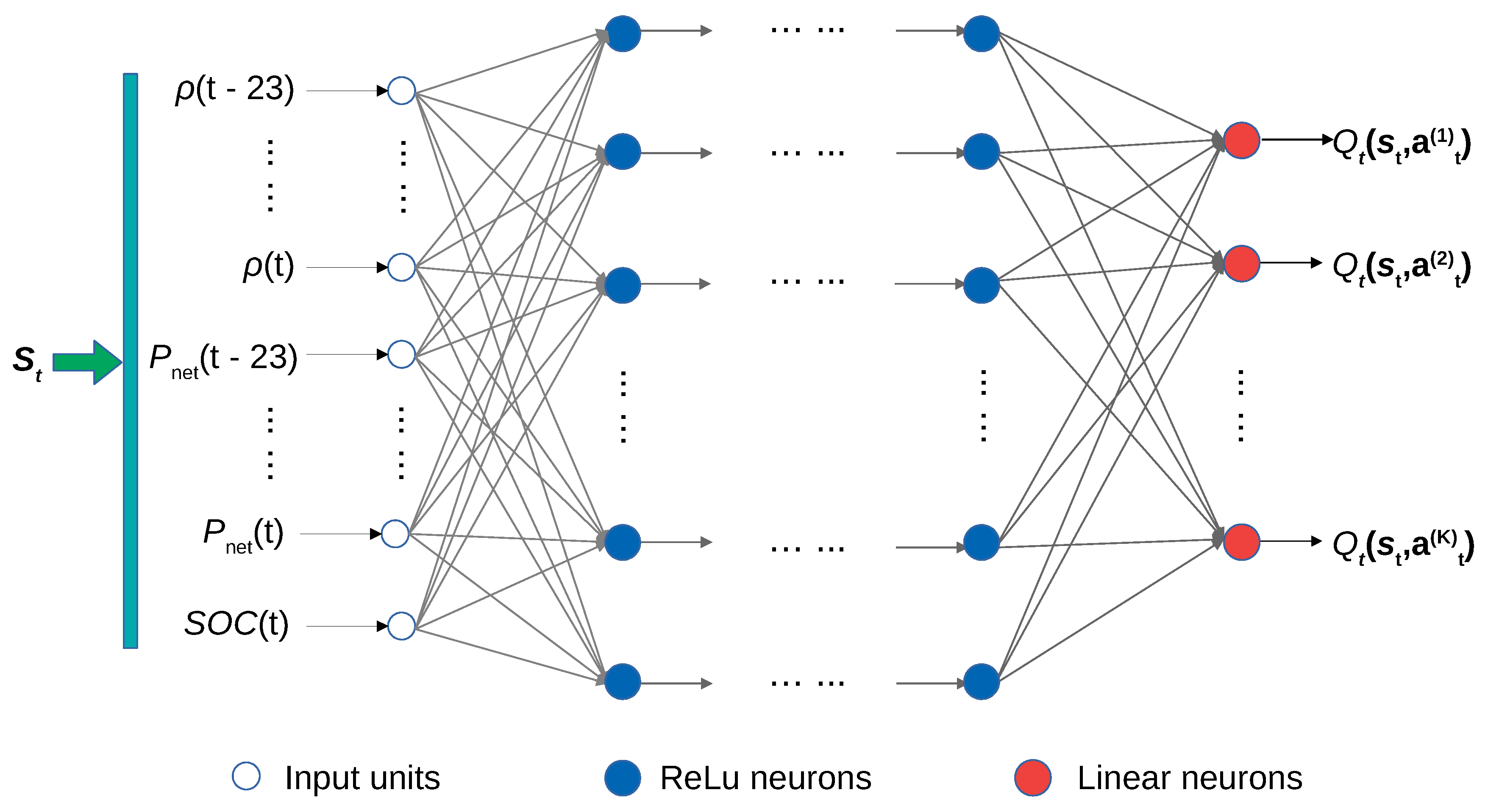
The designed Q-network is presented in Figure 1. The inputs of the Q-network are the MG state s at time step t, and the outputs are the approximate action-values $\tilde{Q}(s,a,\overrightarrow{\mathit{\theta }})$ with respect to the corresponding action a, where $\overrightarrow{\mathit{\theta }}$ represents the set of all connection weights of the neural network. In each hidden layer, every neuron takes all the outputs of the previous layer’s neurons as the inputs of itself. The neuron is formulated by a perceptron model

$${\varphi }_j^l\left(s\right)=\left\{\begin{array}{c}f\left({\sum }_{i=1}^{M_{l-1}}{\theta }_{ij}^l{\varphi }_i^{l-1}\left(s\right)+{\theta }_{0j}^l\right),\mathrm{if}l\ge 1\hfill \\ \hfill \\ f\left({\sum }_{i=1}^{M_{l-1}}{\theta }_{ij}^{l}s+{\theta }_{0j}^l\right),\mathrm{otherwise}\hfill \end{array}\right.$$

(30)

where $f(·)$ is a nonlinear activation function, ${\varphi }_j^l\left(s\right)$ is the output of the jth neuron in the hidden layer $l,l=1,2,\dots ,L$, ${\theta }_{ij}^l$ is the connection weight of the neuron i in the layer $l-1$ to the neuron j in the layer l, and $M_l$ is the number of the neurons in the layer l. To alleviate the gradient-vanish or gradient-explosion problem, the rectified linear unit (ReLU) is adopted as the activation function for each neuron as follows,

$$f\left(x\right)=x^{+}=\left\{\begin{array}{c}x,\mathrm{if}x>0,\hfill \\ 0,\mathrm{otherwise}.\hfill \end{array}\right.$$

(31)

In the output layer is a group of perceptrons with linear activation function, estimating the optimal action-value $Q^{{\pi }^{*}}(s,a^{\left(k\right)})$ for different actions $a^{\left(k\right)},k=1,2,\dots ,K$ given the high-level features extracted by the deep neural network,

$$Q^{{\pi }^{*}}(s,a^{\left(k\right)})=\sum _{i=1}^{M_L}{\theta }_{ik}^l{\varphi }_k^L\left(s\right)+{\theta }_{0k}^L.$$

(32)

By using the backpropagation algorithm, we can calculate the gradient ${▽}_{{\mathit{\theta }}_i}\tilde{Q}(s,a;\overrightarrow{{\mathit{\theta }}_i})$ of the Q-network in Equation (27), and thus train the Q-network.

5. Case Studies

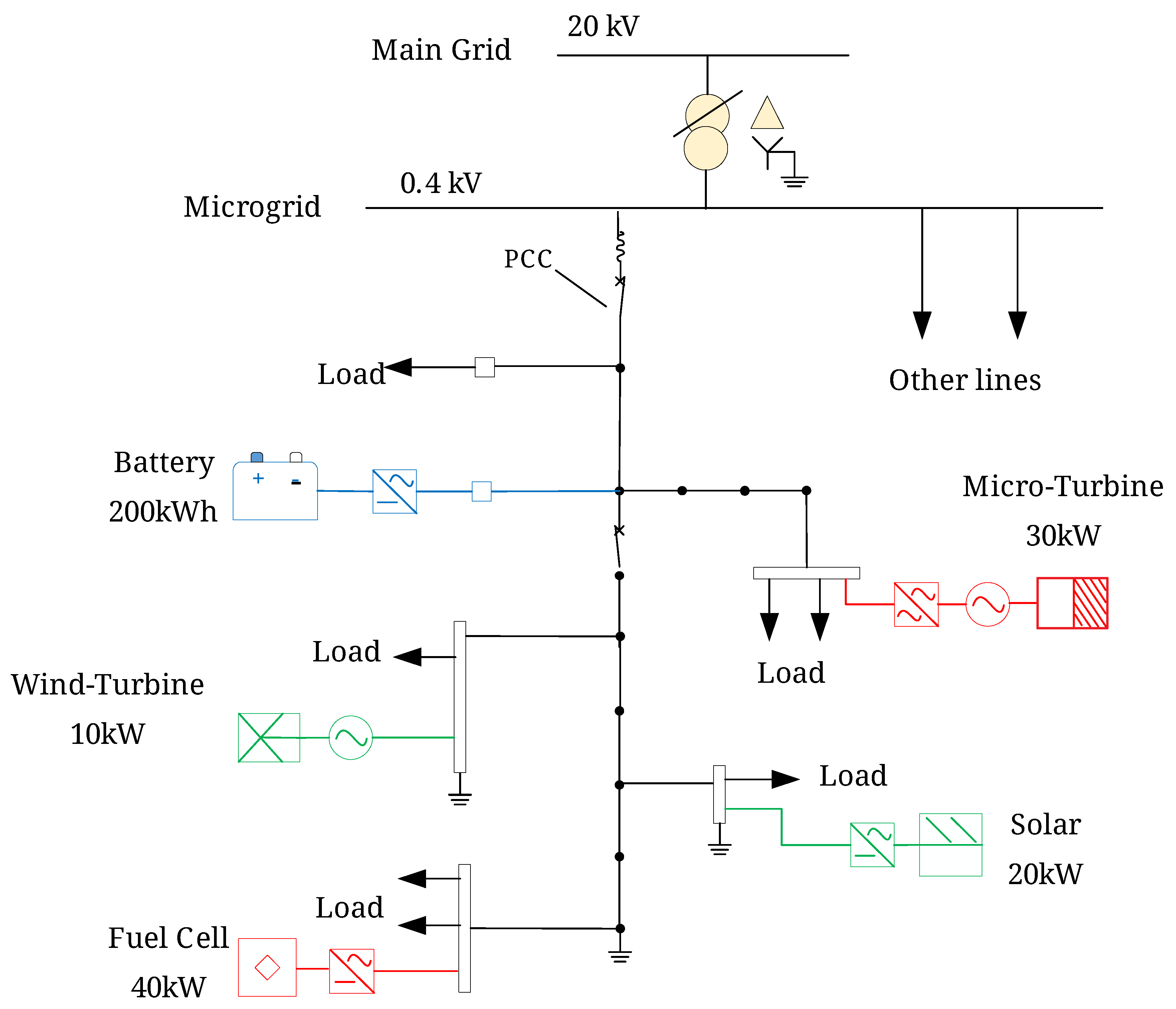
To validate the effectiveness of the proposed DRL approach, we perform simulation studies on the European benchmark low voltage MG system [30]. The structure of the benchmark MG system is shown in Figure 2. The MG consists of a Micro Turbine (MT), a Fuel Cell (FC), a solar photovoltaics (PVs) system, a wind turbine (WT) and a battery ESS and some local loads. The MT and the FC have a maximum output power of 30 kW and 40 kW, respectively. A quadratic cost function is used to model their generation cost. The corresponding coefficients of the cost function for the MG and the FC are shown in

Table 1. Technical constraints and operation parameters of the MG generators and the main grid.

MT	Maximum Power	Minimum Power	Coefficients of cost curve
			Quadratic term	Linear term	Constant term
	$P_{DG}^{1,max}=30$ kW	$P_{DG}^{1,min}=0$ kW	$a_1=0.01$	$a_2=7.16$	$a_3=4.615$
FC	Maximum Power	Minimum Power	Coefficients of cost curve
			Quadratic term	Linear term	Constant term
	$P_{DG}^{2,max}=40$ kW	$P_{DG}^{2,min}=0$ kW	$a_1=0.01$	$a_2=5.04$	$a_3=11.011$
ESS	Maximum SOC	Minimum SOC	Capacity	Maximum Power
				Charging	Discharging
	$SO{C}_{min}=1.0$	$SO{C}_{min}=0.15$	$E_b=200$ kWh	$P_b^{ch,max}=50$ kW	$P_b^{dis,max}=50$ kW
Grid	Maximum Power	Discount factor of selling prices		–	–
	$P_g^{max}=200$ kW	$\beta =0.1$		–	–

. The capacity of the ESS is 200 kWh, and its minimum and maximum SOC are 0.15 and 1.0, respectively. The charging and discharging efficiencies are 0.98. The charging/discharging power of the ESS is uniformly discretized to $k=101$ values in the interval [−50 kW, 50 kW]. The limit of exchanged power at PCC is 200 kW. The parameters of the ESS and the main grid are presented in Table 1. The maximal power production of the PVs and the WT is 20 kW and 10 kW, respectively. The time interval $\Delta t$ between two time steps is 1 h.

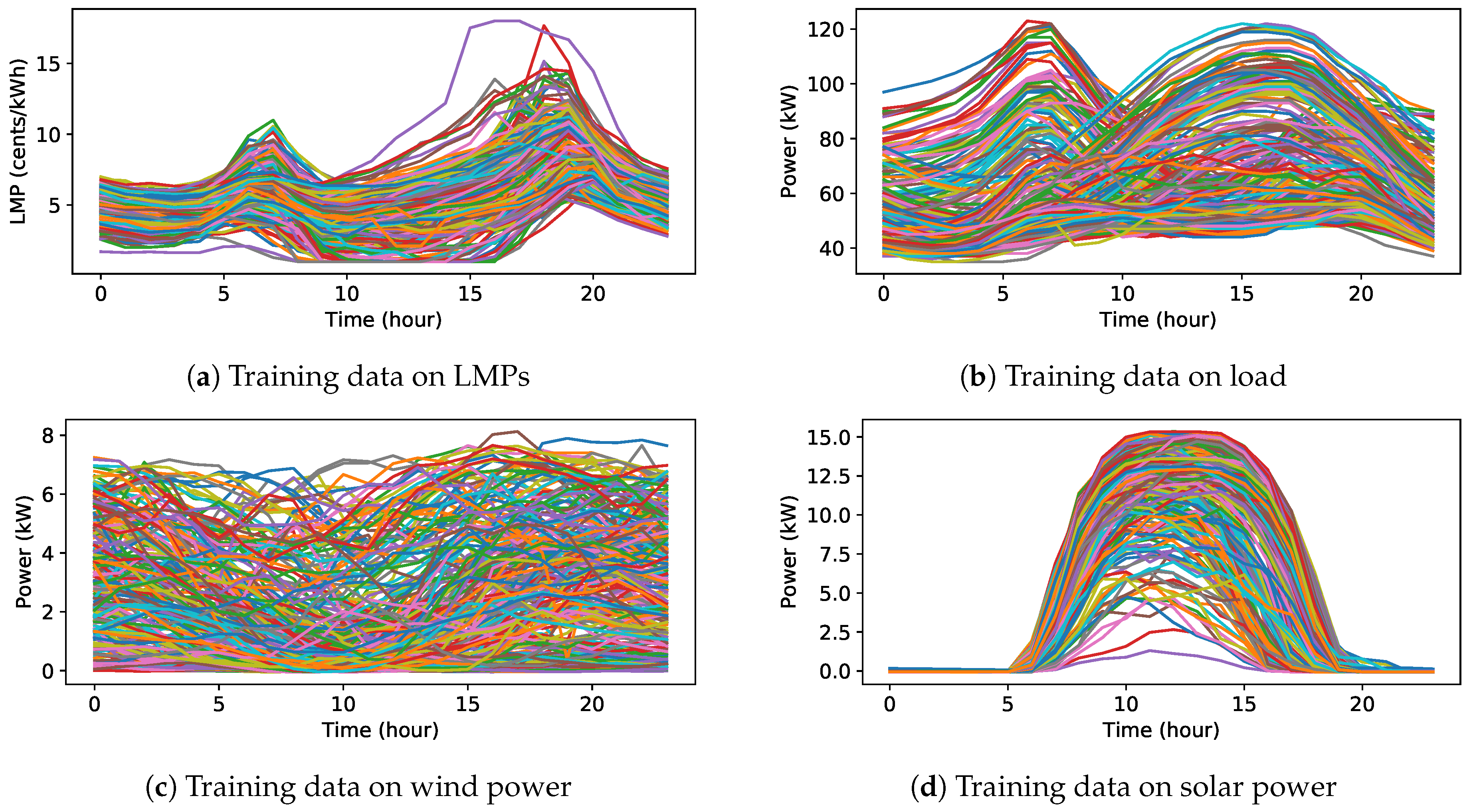
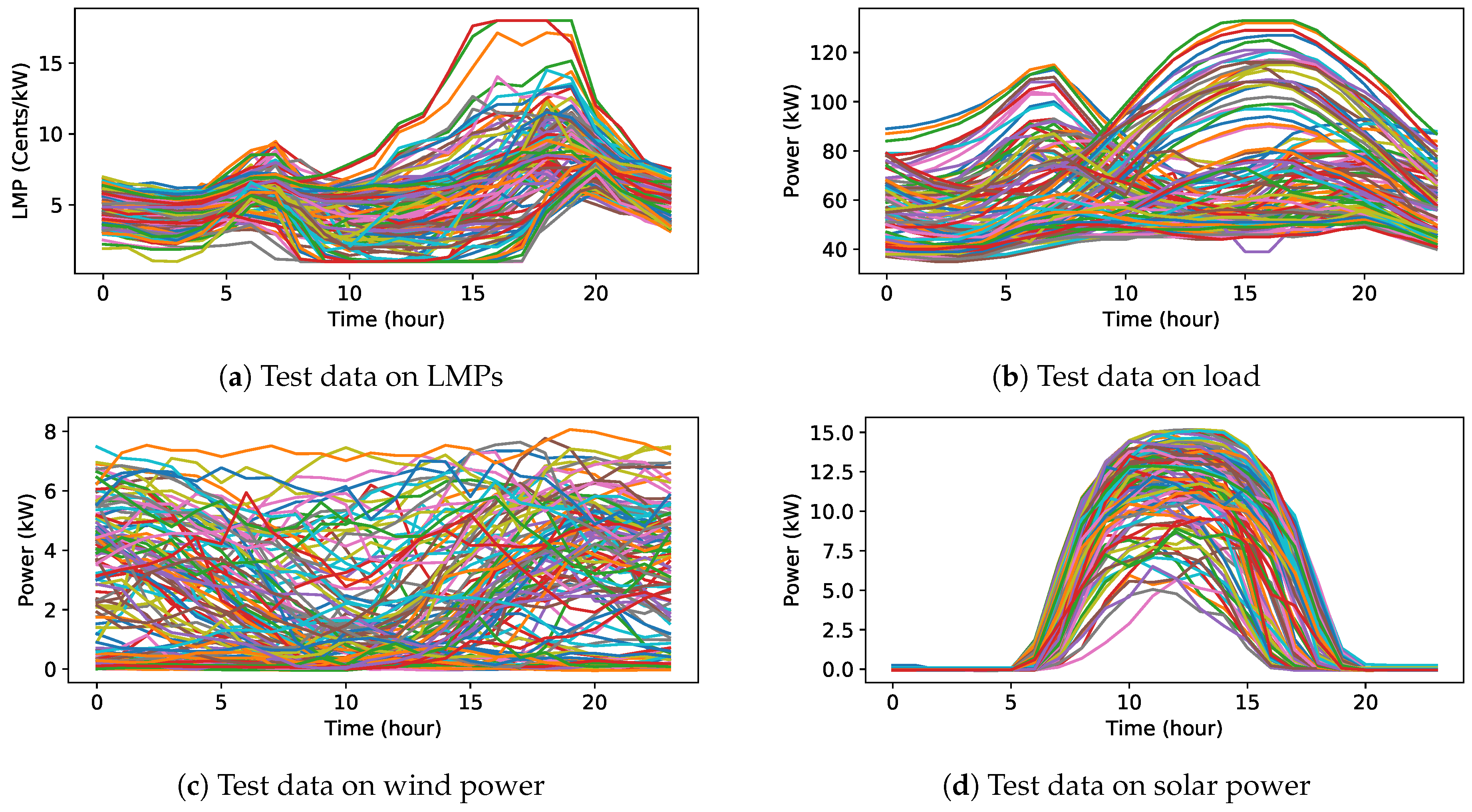
We evaluate the proposed DRL approach on two experiments. In the first experiment, the proposed approach is tested in a deterministic scenario. In this scenario, the WT generation, PVs production, load demand, and LMPs over a period of one day are known, but the SOC of the ESS is initialized with different values. This is to show that the proposed DRL method can learn to make effective schedules in a deterministic environment for any initial state of the ESS. In the second experiment, we apply real power system data on wind generation, PVs production, load demand and LMP from the CAISO [31] over a period of one-year to the proposed approach. We use the first 21 days in each month as the training set and the remaining days in each month as the test set. This is to demonstrate that the proposed DRL method is adaptive to stochastic scenarios and able to generalize well to situations that it has never seen.

In both experiments, the proposed DRL approach is implemented in Tensorflow 1.12, an open source deep learning platform. The simulations are carried out on a personal computer with 4 Intel (R) Cores (TM) i5-6300U CPU, 2.40 GHz and 8 GB RAM memory. The simulation environment is Python 3.6.8.

5.1. Experiment 1: Deterministic Scenario

In this experiment, the Q-network has 3 fully connected hidden layers. Each hidden layer has 200 ReLU neurons. The output layer is also a fully connected layer with 101 linear neurons. Overall, there are $110,000$ connection weights and 600 hidden neurons. All the weights are initiated to zero-mean Gaussian with a variance of 0.01. The capacity N of the replay memory $\mathcal{D}$ is set to be 5000, and the minibatch size of samples is 240 for each gradient descent step.

We run the DQN algorithm (Algorithm 1) 1000 episodes for training in this experiment. In the first 100 episodes, actions are chosen at total random to try to explore the state-action space as well as possible. Afterwards, the $ϵ$-greedy policy in Equation (26) is used to choose actions. From episode 101 to episode 900, the value of $ϵ$ gradually decreases from 1.0 to 0.1 to keep a balance between exploration and exploitation. Then, the value of $ϵ$ stays at 0.1 until the end of training.

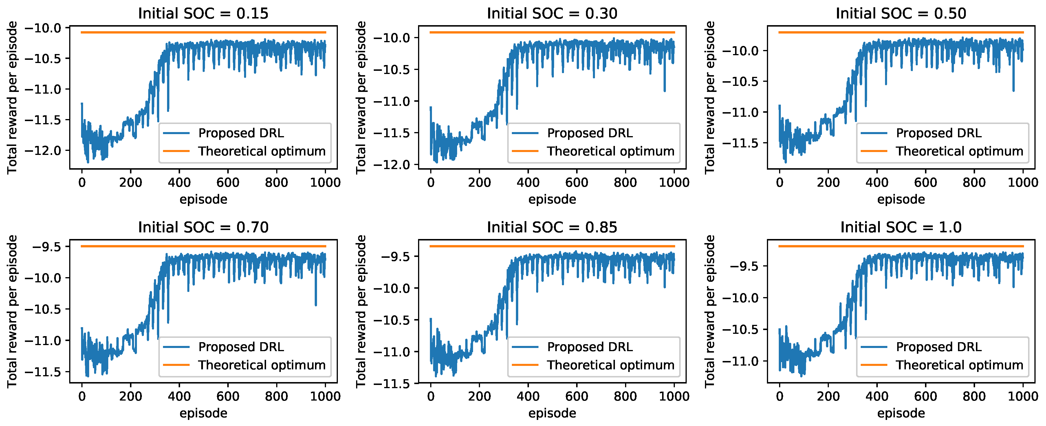
We evaluated the proposed approach periodically in the course of training by testing it without exploration, e.g., setting $ϵ=0$ and choosing actions greedily to maximize the action-value function. We compare the performance of the proposed approach with that of the theoretical optimum strategy. The theoretical optimum strategy formulates the problem as a mixed-integer nonlinear programming problem. Then, the problem is modeled by using the YALMIP toolbox [32] and solved via a built-in solver named “BMIBNB” to obtain the best generation schedules. Figure 3 shows the performance curves of the proposed approach with different initial values of the SOC of the ESS. As shown in the figure, the proposed approach succeeds in learning to increase the rewards on different initial SOC states of the ESS. After about 400 episodes, all the performance curves reach their highest values, and converge to a small area that is very close to the corresponding theoretical optimum, respectively.

Table 2. Comparison of the operating costs obtained by the proposed DRL and the theoretical optimum.

Initial SOC	0.15	0.2	0.25	0.3	0.35	0.4	0.45	0.5	0.55
DQL	$102.85	$102.40	$101.72	$101.49	$100.49	$100.11	$100.36	$99.66	$98.75
Optimum	$100.77	$100.23	$99.70	$99.17	$98.63	$98.10	$97.57	$97.03	$96.52
Initial SOC	0.6	0.65	0.7	0.75	0.8	0.85	0.9	0.95	1.0
DQL	$97.98	$97.28	$96.92	$97.20	$96.59	$95.50	$94.95	$94.20	$93.63
Optimum	$96.00	$95.49	$94.97	$94.46	$93.94	$93.43	$92.91	$92.40	$91.89

compares the rewards obtained by the proposed DRL approach and the theoretical optimum strategy in details. On average, the performance gap between the proposed DRL approach and the theoretical optimum is $2.16, only accounting for 2.2% of the total cost.

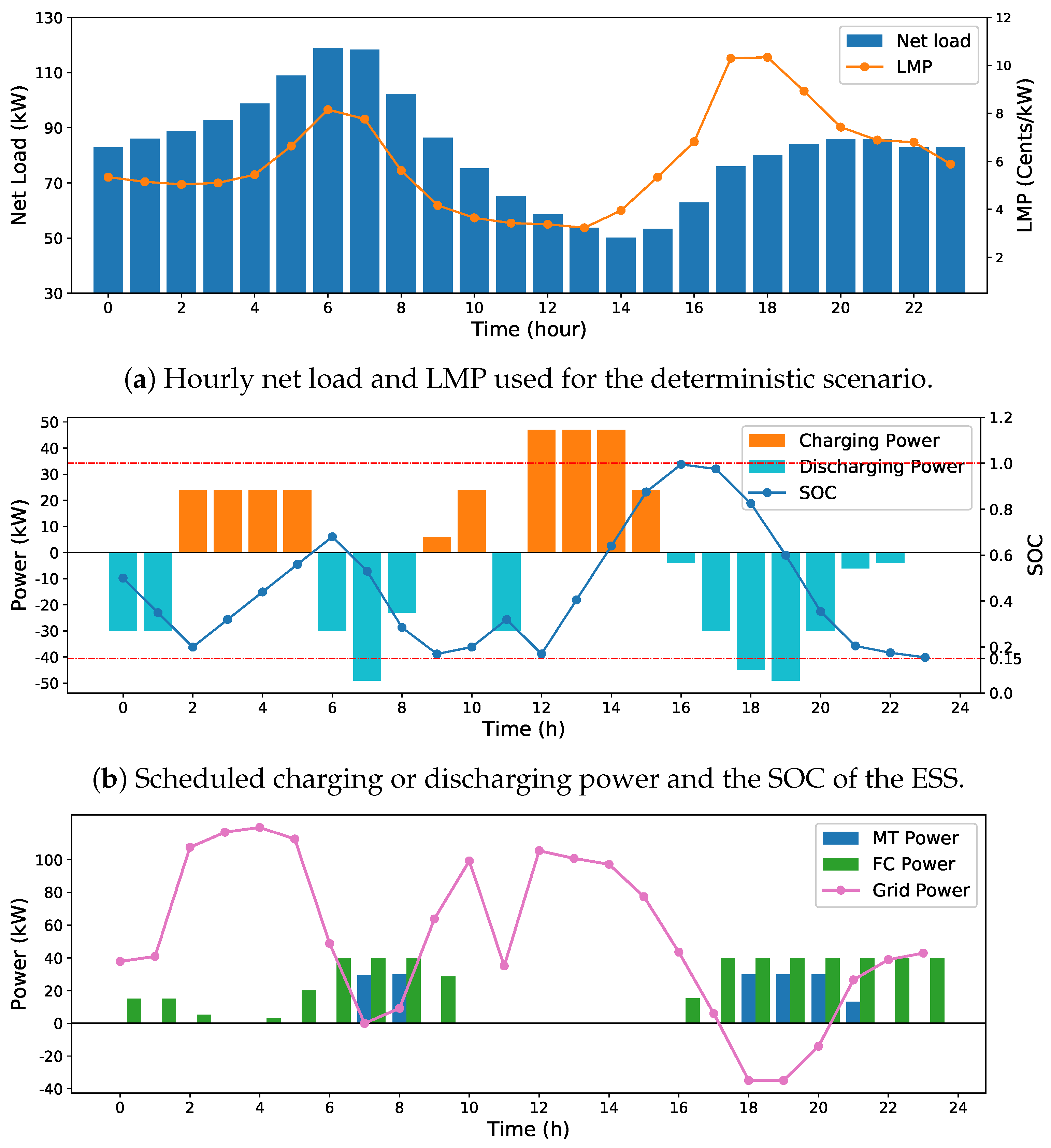
Figure 4a shows the hourly LMPs and net load over a period of one day. Figure 4b,c presents the scheduling results obtained by the DRL approach. The initial SOC of the ESS is 0.5. As it can be seen in Figure 4b, the ESS is charged during low LMP periods, from hour 2 to 6 and hour 9 to 15. Correspondingly, the SOC level increases at the same time. During high LMP periods, from hour 6 to 8 and hour 16 to 22, the ESS is discharged to help supply the local demand or sell the electricity to the main grid. This pattern coincides with the curve of power exchanged with the main grid as presented in Figure 4c. When the LMPs are relatively low, the MG purchases electricity from the main grid to supply the local demand and charge the ESS. In addition, the power outputs of the MT or the FC are reduced if the LMPs are lower than their generating costs. When the LMPs are high, however, the MG imports less electricity. The FC and the MT are scheduled to generate power because they are less costly. These simulation results demonstrate that the proposed DRL approach can learn a cost-effective scheduling strategy on different initial conditions of the ESS.

5.2. Experiment 2: Stochastic Scenario

In this experiment, we consider the MG in a more realistic setting where the load demand, RES production, and LMP are stochastic. The proposed DRL approach is evaluated by using real power system data in 2016 from the CAISO. We use the first 21 days in each month as the training set and the remaining days in 2016 as the test set. In total, there are 252 days of hourly data in the training set and 114 days of hourly data in the test set, respectively. The used data in the experiment are presented in Figure 5 and Figure 6. The Q-network consists of 3 fully connected hidden layers. Each hidden layer has 500 ReLU neurons. The output layer is a fully connected layer with 101 linear neurons. Overall, there are 575,000 connection weights and 1500 hidden neurons. All the weights are initialized to zero-mean Gaussian with a variance of 0.01. The capacity N of the replay memory $\mathcal{D}$ is set to be 20,000, and the minibatch size of samples is 240 for each gradient descent step. We run the DQN algorithm (Algorithm 1) 15,000 episodes for training. In the first 1000 episodes, actions are chosen at total random to try to explore the state-action space. Then, the $ϵ$-greedy policy is used to choose actions with a decaying $ϵ$. From episode 1001 to episode 9000, the value of $ϵ$ gradually decreases from 1.0 to 0.1 to keep a balance between exploration and exploitation. After that, the value of $ϵ$ stays at 0.1 until the end of the training.

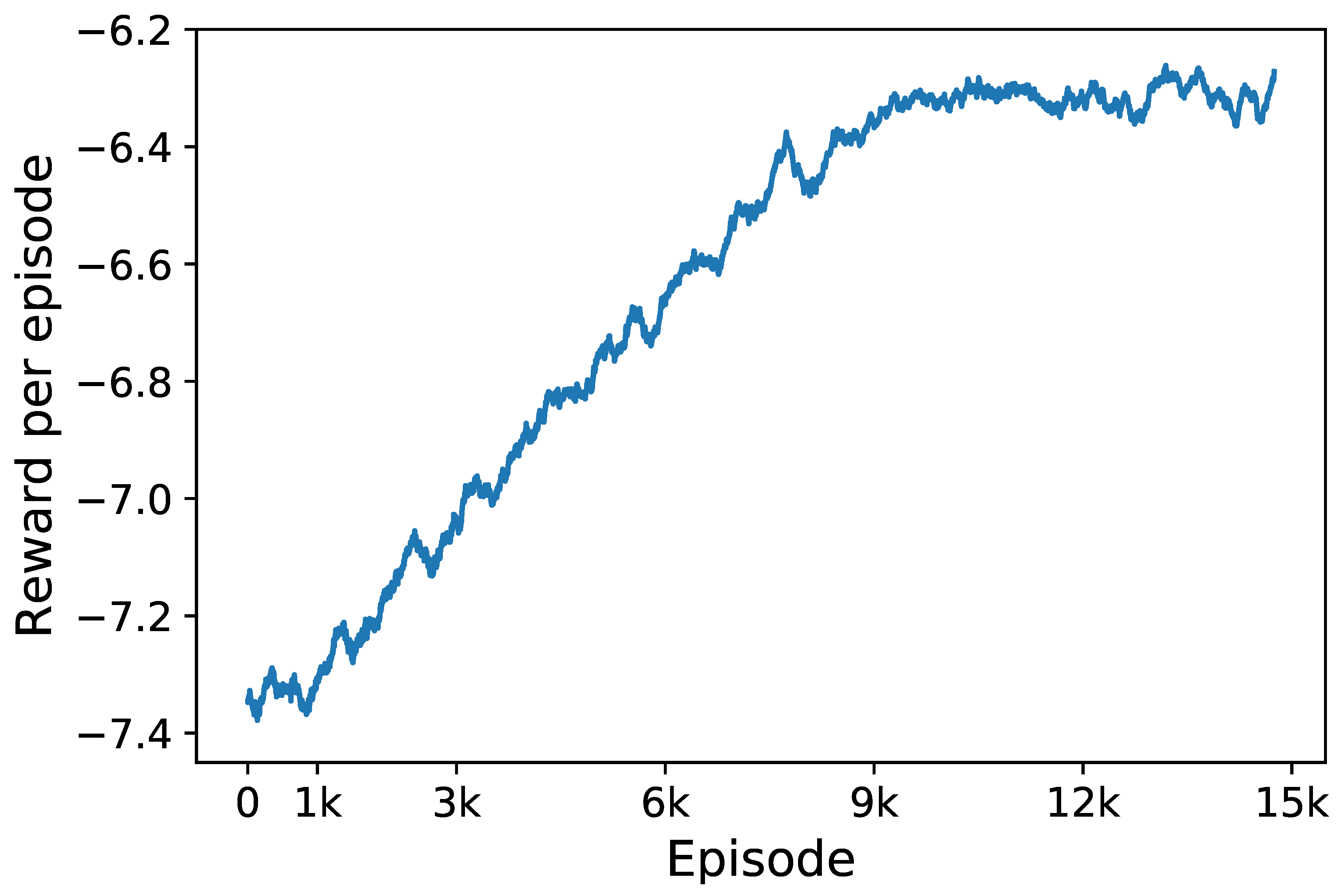
During the training process, we calculate the total rewards ${\sum }_{t=1}^T{r}_t$ at each episode to monitor the learning performance of the proposed approach. Figure 7 presents the learning curve of the proposed approach. As shown in the figure, for the first 1000 episodes when the agent selects actions at total random, the rewards vary in the range from −7.4 to −7.3. From episode 1000 to 9000, the rewards gradually increase from −7.35 to −6.3. After 9000 episodes, the cumulative rewards converge to a small region around −6.3. This result demonstrates that the proposed approach succeeds in learning an effective and stable policy under the stochastic environment.

To evaluate the performance of the proposed approach in the test set, several benchmark solutions are applied for comparison. The benchmark solutions include (1) theoretical optimum; (2) standard Q-learning (SQL); (3) fitted Q-iteration (FQI); and (4) uncontrolled strategy. For the theoretical optimum solution, we assume that the LMPs and net load of the MG are known in advance, and the problem is modeled as a mixed-integer nonlinear programming. The build-in solver “BMIBNB” in YALMIP toolbox [32] is employed to solve the model. Please note that the theoretical optimum solution provides the minimal daily operating cost of the MG, but it can never be reached in practice due to the existence of uncertainty. For the SQL solution, a neural network with one hidden layer is used to approximate the optimal action-value function. The hidden layer consists of 1000 ReLU neurons. The standard Q-learning algorithm is employed to train the neural network and the greedy policy is used to select actions while making real-time scheduling decisions. Through trial and error, we set the maximum training episode to be 5000 for the best performance. For the FQI solution, a linear approximator is used to approximate the action-value function. The batch size for training the approximator is set to be 15,000 for comparison. Similarly, the generation schedules are determined based on the greedy policy that selects actions maximizing the approximate action-value function. For the uncontrolled strategy, the MG supplies its local demand all by purchasing electricity from the main grid no matter what the LMP is. The uncontrolled strategy serves as a baseline for the performance evaluation in the test set.

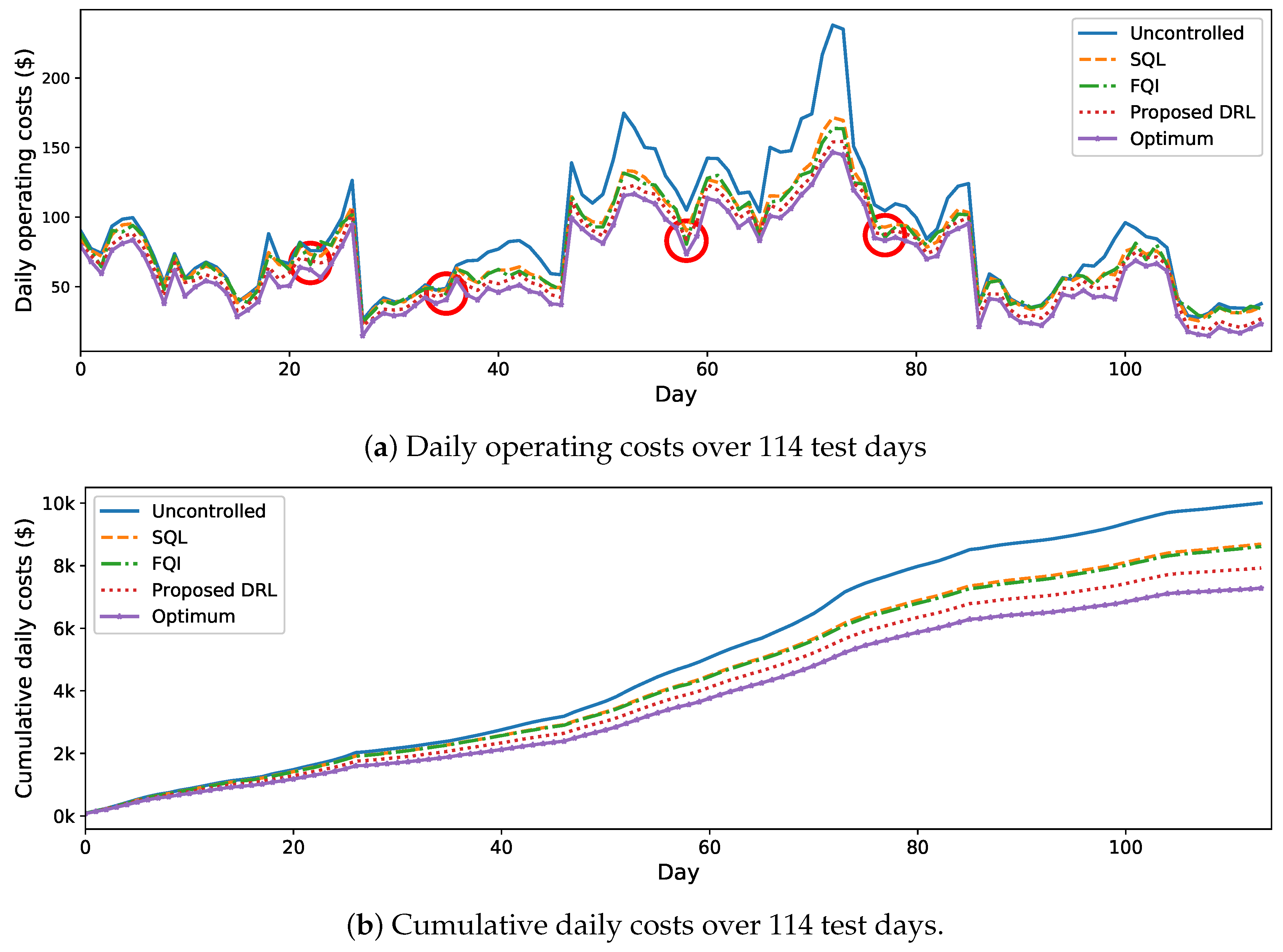
The daily operating costs of the MG and the corresponding cumulative daily costs on the test days by using the proposed and benchmark solutions are presented in Figure 8. As it can be seen in Figure 8a, the proposed approach obtained lower daily operating costs on most of the test days than the benchmarks. Although there are bad cases (marked by red circles) on several test days where the proposed approach does not obtain as good results as the other benchmarks, the overall performance of the proposed approach is better. As shown in Figure 8b, in terms of the cumulative daily costs, the proposed DRL approach outperforms the other two RL solutions and obtains a lower total operating cost over all test days. Compared with the uncontrolled strategy (blue dotted line), the proposed DRL approach (red dotted line) reduces the operating cost by 20.75%, but the SQL (orange dash line) and FQI (green dash-dotted line) solutions only reduce the operating cost by 13.12% and 13.92%, respectively. Furthermore, the performance of the proposed approach is close to the theoretical optimum. The cost reduction by the proposed approach is only 6.45% less than the one resulted from the theoretical optimum strategy (purple star). These results demonstrate the effectiveness of the proposed DRL approach for real-time energy management of a MG with uncertainty.

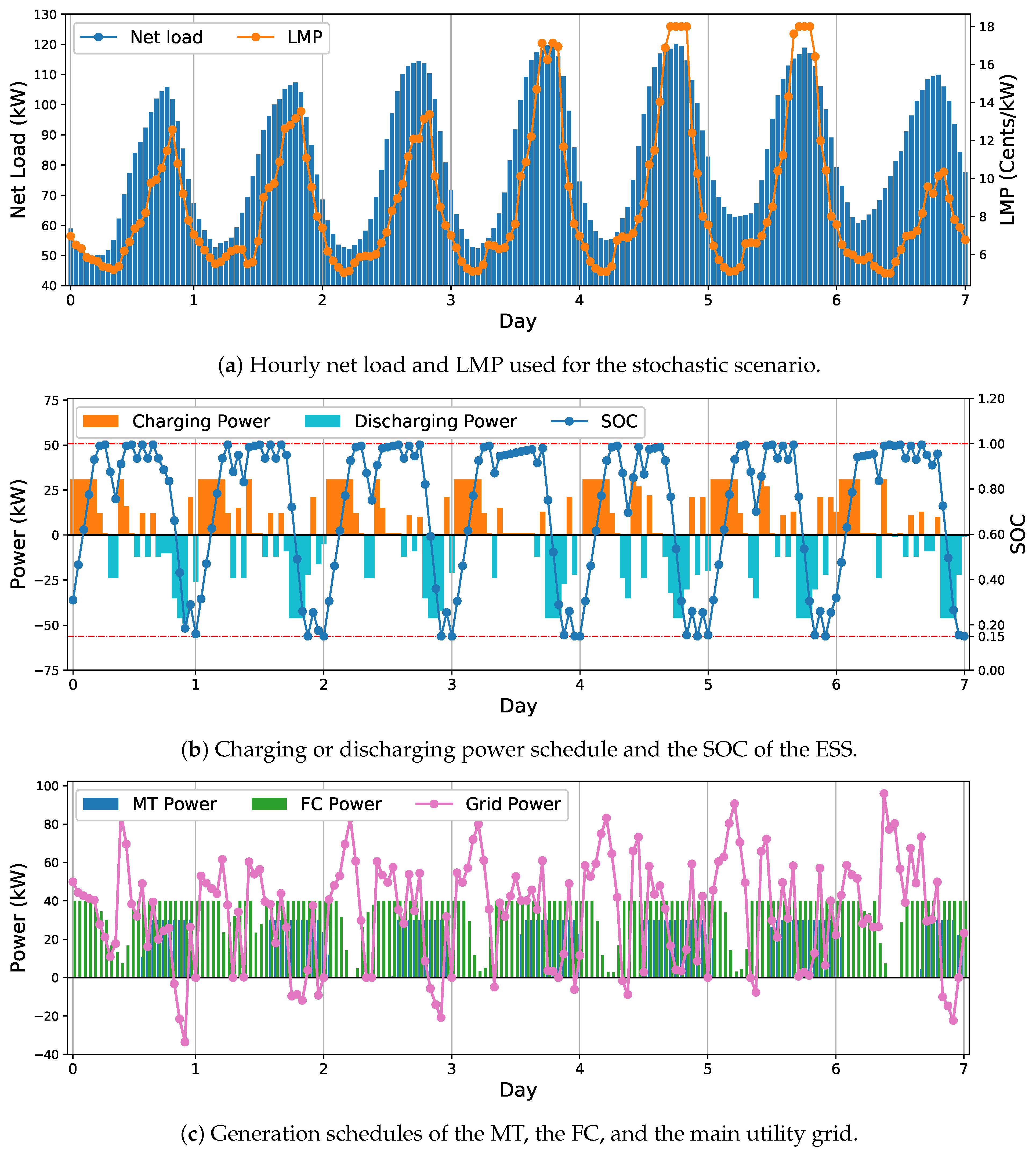
To further investigate the performance of the proposed approach, the yielded generation schedules over 7 consecutive days in the test results are presented in Figure 9. In Figure 9a, the hourly LMPs and net load over the 7 days are illustrated. The charging/discharging power schedule and the SOC of the ESS are presented in Figure 9b. As it can be observed, the ESS is charged when the LMPs and net load are at peak, and discharged when they are off peak. This means that the proposed approach can effectively manage the charging or discharging of the ESS. By taking advantage of its buffer effect, the low-budget electricity is stored at off-peak hours, and then discharged at peak hours to supply the local demand or sold to the main grid. Moreover, the SOC of the ESS at the end of each day is equivalent or close to its minimum admissible value, i.e., 0.15. This means that the proposed approach can sufficiently use the energy of the ESS by the end of the scheduling over a day to minimize the daily operating cost. For the utility grid, as shown in Figure 9c, the MG purchases less electricity from the main grid at peak hours to save cost or sell extra electricity to it to earn revenue. This is because that superfluous power is purchased at low LMP hours and stored in the ESS. A similar pattern can be observed from the schedules of the MT and FC in this figure. The MT or the FC generates electricity when the LMPs are higher than the corresponding generation cost, and reduce the generation when the LMPs are lower. The simulation results demonstrate that the proposed approach can adaptively adjust its actions to the trends of the LMP and net load, and make cost-effective schedules for operating the MG under uncertain environments.

5.3. Analysis: Effect of Hyper-Parameters

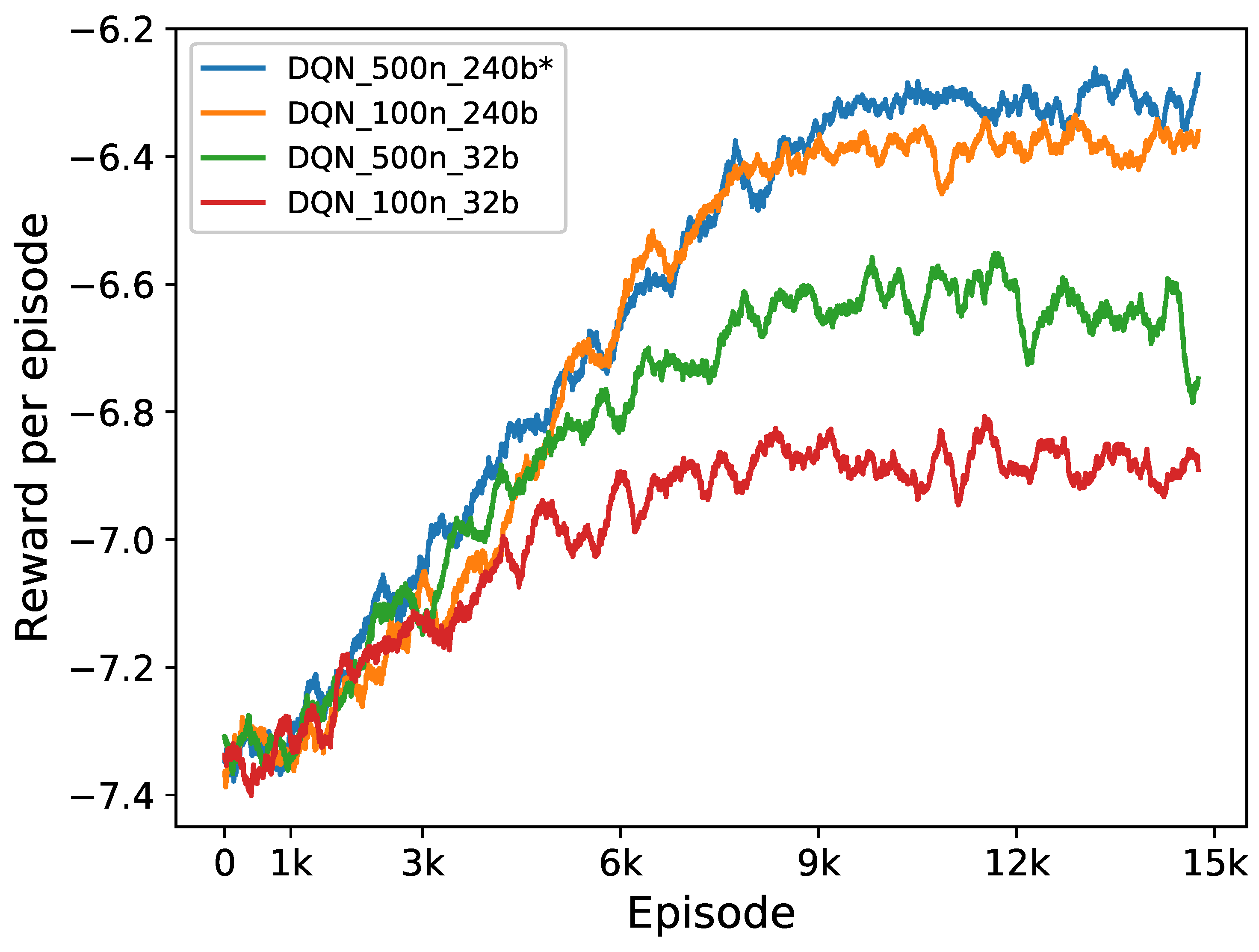
To demonstrate how the hyper-parameters affect the performance of the proposed DRL approach, we train the DRL approach using different hyper-parameters and then test it in the stochastic scenario. Specifically, we apply three sets of different hyper-parameters to the DRL approach. (1) In the first set of hyper-parameters, the number of neurons in each hidden layer of the Q-network is reduced from 500 to 100, and the other hyper-parameters remain unchanged. We refer the DRL approach using this set of hyper-parameters to as DQN-100n-240b, where “100n” denotes 100 neurons in each hidden layer, and “240b” denotes the batch size for training the Q-network is 240; (2) In the second set of hyper-parameters, the number of neurons in each hidden layer of the Q-network is still 500, but the batch size for training the Q-network is reduced from 240 to 32, and the other hyper-parameters remain unchanged. We refer the DRL using this set of hyper-parameters to as DQN-500n-32b; (3) In the third set of hyper-parameters, the number of neurons in each hidden layer of the Q-network is changed from 500 to 100, and the batch size for training the Q-network is also changed from 240 to 32. We refer the DRL using this set of hyper-parameters to as DQN-100n-32b.

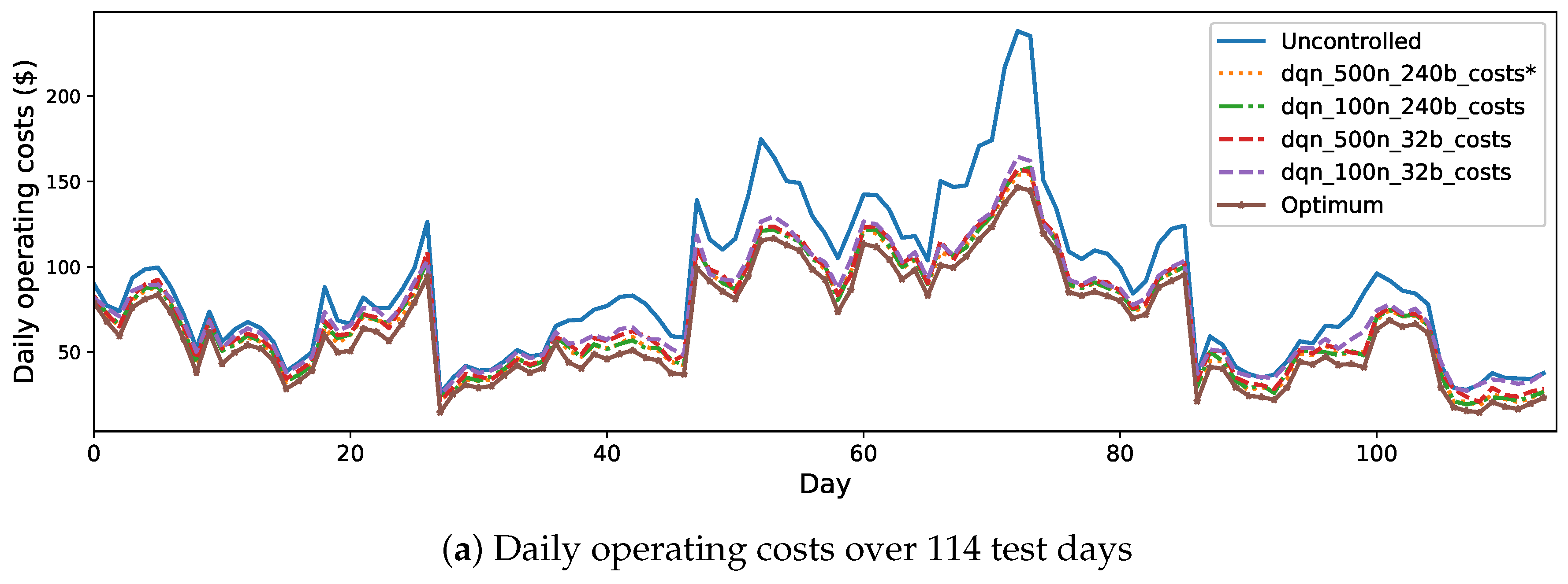
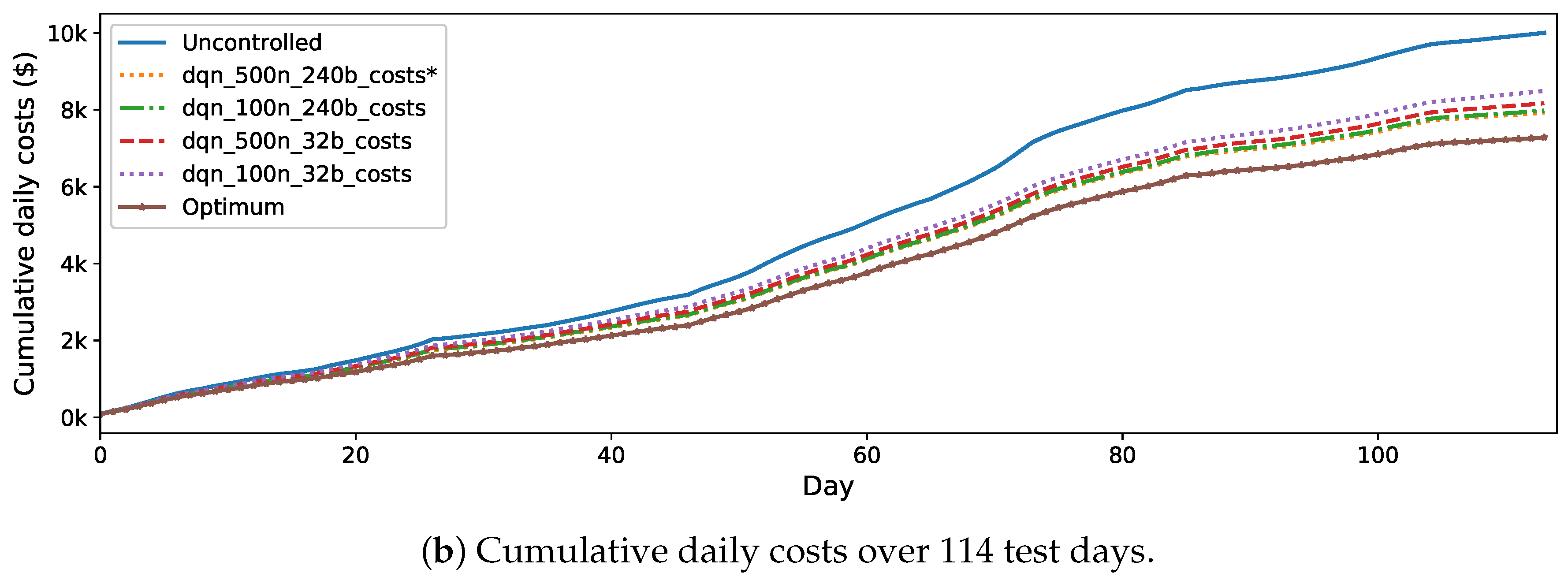
Figure 10 shows the learning curves of the proposed DRL approach and the DRL with the three different sets of hyper-parameters mentioned above. Figure 11 shows the daily operating costs and the corresponding cumulative daily costs on the test set. In both Figure 10 and, the proposed DRL approach is referred to as DQN-500n-240b and marked by “∗”. As shown in these figures, using less hidden neurons in the Q-network or/and less batch size for training, the performance of the DRL approach degrades, in both the training process and the test results. Comparatively, reducing the batch size from 240 to 32 has a worse influence on the performance than reducing the number of hidden neurons of the Q-network from 500 to 100. This could be because that when we reduce the batch size, the number of samples used at each iteration for training the Q-network becomes less. Therefore, we may run the risk of not taking full advantage of the samples in the replay buffer and resulting in an underestimated Q-network.

6. Conclusions

This paper has presented a learning-based energy management approach for real-time scheduling of a MG. The uncertainty of the load demand, renewable energy, and electricity price are considered in the proposed approach. Specifically, the MG real-time scheduling problem is formulated as an MDP model. The objective is to find an optimal scheduling strategy to minimize the daily operating cost of the MG. A DRL approach that does not require an explicit model of the uncertainty is developed to solve the MDP. In the proposed approach, the DQN algorithm and a carefully designed deep feedforward neural network are used to approximate the action-value function. The proposed approach takes the state of MG as the inputs, and outputs directly the real-time generation schedules. The performance of the DRL approach has been evaluated using real power-grid data from CAISO. Simulation results showed that the proposed DRL approach could outperform the traditional RL approaches on the considered problem and predict the trend of the uncertainty without an explicit model. Analysis of the scheduling results on the test dataset demonstrated that the proposed approach could adaptively adjust its actions to the trends of the LMP and net load, and make cost-effective schedules for operating the MG under uncertain environments.

References

- Energy.Gov. About the Grid Modernization Initiative. Available online: https://www.energy.gov/grid-modernization-initiative (accessed on 10 January 2019).
- Farhangi, H. The path of the smart grid. IEEE Power Energy Mag. 2010, 8, 18–28. [Google Scholar] [CrossRef]
- Fang, X.; Misra, S.; Xue, G.; Yang, D. Smart Grid—The New and Improved Power Grid: A Survey. IEEE Commun. Surv. Tutor. 2012, 14, 944–980. [Google Scholar] [CrossRef]
- Galli, S.; Scaglione, A.; Wang, Z. For the Grid and Through the Grid: The Role of Power Line Communications in the Smart Grid. Proc. IEEE 2011, 99, 998–1027. [Google Scholar] [CrossRef]
- Lasseter, R.H. Microgrids. In Proceedings of the 2002 IEEE Power Engineering Society Winter Meeting Conference Proceedings, New York, NY, USA, 27–31 January 2002; pp. 305–308. [Google Scholar]
- Kaur, J.K.A.; Basak, P. A review on microgrid central controller. Renew. Sustain. Energy Rev. 2016, 55, 338–345. [Google Scholar] [CrossRef]
- Zhao, B.; Xue, M.; Zhang, X.; Wang, C.; Zhao, J. An MAS based energy management system for a stand-alone microgrid at high altitude. Appl. Energy 2015, 143, 251–261. [Google Scholar] [CrossRef] [Green Version]
- Bacha, S.; Picault, D.; Burger, B.; Etxeberria-Otadui, I.; Martins, J. Photovoltaics in Microgrids: An Overview of Grid Integration and Energy Management Aspects. IEEE Ind. Electron. Mag. 2015, 9, 33–46. [Google Scholar] [CrossRef]
- Zhou, H.; Bhattacharya, T.; Tran, D.; Siew, T.S.T.; Khambadkone, A.M. Composite Energy Storage System Involving Battery and Ultracapacitor With Dynamic Energy Management in Microgrid Applications. IEEE Trans. Power Electron. 2011, 26, 923–930. [Google Scholar] [CrossRef]
- Xu, L.; Chen, D. Control and Operation of a DC Microgrid With Variable Generation and Energy Storage. IEEE Trans. Power Deliv. 2011, 26, 2513–2522. [Google Scholar] [CrossRef]
- Patterson, M.; Macia, N.F.; Kannan, A.M. Hybrid Microgrid Model Based on Solar Photovoltaic Battery Fuel Cell System for Intermittent Load Applications. IEEE Trans. Energy Conv. 2015, 30, 359–366. [Google Scholar] [CrossRef]
- Thirugnanam, K.; Kerk, S.K.; Yuen, C.; Liu, N.; Zhang, M. Energy Management for Renewable Microgrid in Reducing Diesel Generators Usage With Multiple Types of Battery. IEEE Trans. Ind. Electron. 2018, 65, 6772–6786. [Google Scholar] [CrossRef]
- Lawder, M.T.; Suthar, B.; Northrop, P.W.; De, S.; Hoff, C.M.; Leitermann, O.; Crow, M.L.; Santhanagopalan, S.; Subramanian, V.R. Battery Energy Storage System (BESS) and Battery Management System (BMS) for Grid-Scale Applications. Proc. IEEE 2014, 102, 1014–1030. [Google Scholar] [CrossRef]
- Petrollese, M.; Valverde, L.; Cocco, D.; Cau, G.; Guerra, J. Real-time integration of optimal generation scheduling with MPC for the energy management of a renewable hydrogen-based microgrid. Appl. Energy 2016, 166, 96–106. [Google Scholar] [CrossRef]
- Craparo, E.; Karatas, M.; Singham, D.I. A robust optimization approach to hybrid microgrid operation using ensemble weather forecasts. Appl. Energy 2017, 201, 135–147. [Google Scholar] [CrossRef]
- Li, Z.; Zang, C.; Zeng, P.; Yu, H. Combined Two-Stage Stochastic Programming and Receding Horizon Control Strategy for Microgrid Energy Management Considering Uncertainty. Energies 2016, 9, 499. [Google Scholar] [CrossRef]
- Morstyn, T.; Hredzak, B.; Aguilera, R.P.; Agelidis, V.G. Model Predictive Control for Distributed Microgrid Battery Energy Storage Systems. IEEE Trans. Control. Syst. Technol. 2018, 26, 1107–1114. [Google Scholar] [CrossRef]
- Mbuwir, B.; Ruelens, F.; Spiessens, F.; Deconinck, G. Battery Energy Management in a Microgrid Using Batch Reinforcement Learning. Energies 2017, 10, 1846. [Google Scholar] [CrossRef]
- Kim, S.; Lim, H. Reinforcement Learning Based Energy Management Algorithm for Smart Energy Buildings. Energies 2018, 11, 2010. [Google Scholar] [CrossRef]
- Venayagamoorthy, G.K.; Sharma, R.K.; Gautam, P.K.; Ahmadi, A. Dynamic Energy Management System for a Smart Microgrid. IEEE Trans. Neural Netw. Learn. Syst. 2016, 8, 1643–1656. [Google Scholar] [CrossRef]
- Foruzan, E.; Soh, L.; Asgarpoor, S. Reinforcement Learning Approach for Optimal Distributed Energy Management in a Microgrid. IEEE Trans. Power Syst. 2018, 33, 5749–5758. [Google Scholar] [CrossRef]
- Mnih, V.; Kavukcuoglu, K.; Silver, D.; Rusu, A.A.; Veness, J.; Bellemare, M.G.; Graves, A.; Riedmiller, M.; Fidjeland, A.K.; Ostrovski, G.; et al. Human-level control through deep reinforcement learning. Nature 2015, 518, 529–533. [Google Scholar] [CrossRef]
- Silver, D.; Huang, A.; Maddison, C.J.; Guez, A.; Sifre, L.; Driessche, G.V.D.; Schrittwieser, J.; Antonoglou, I.; Panneershelvam, V.; Lanctot, M.; et al. Mastering the game of go with deep neural networks and tree search. Nature 2016, 529, 484–489. [Google Scholar] [CrossRef] [PubMed]
- François-Lavet, V.; Taralla, D.; Ernst, D.; Fonteneau, R. Deep reinforcement learning solutions for energy microgrids management. In Proceedings of the 13th European Workshop on Reinforcement Learning (EWRL 2016), Barcelona, Spain, 3–4 December 2016. [Google Scholar]
- Zeng, P.; Li, H.; He, H.; Li, S. Dynamic Energy Management of a Microgrid using Approximate Dynamic Programming and Deep Recurrent Neural Network Learning. IEEE Trans. Smart Grid 2018, in press. [Google Scholar] [CrossRef]
- Gibilisco, P.; Ieva, G.; Marcone, F.; Porro, G.; Tuglie, E.D. Day-ahead operation planning for microgrids embedding Battery Energy Storage Systems. A case study on the PrInCE Lab microgrid. In Proceedings of the 2018 AEIT International Annual Conference, Bari, Italy, 3–5 October 2018; pp. 1–6. [Google Scholar]
- Zhang, Y.; Zhang, T.; Wang, R.; Liu, Y.; Guo, B. Optimal operation of a smart residential microgrid based on model predictive control by considering uncertainties and storage impacts. Sol. Energy 2015, 122, 1052–1065. [Google Scholar] [CrossRef]
- Cagnano, A.; Bugliari, A.C.; Tuglie, E.D. A cooperative control for the reserve management of isolated microgrids. Appl. Energy 2018, 218, 256–265. [Google Scholar] [CrossRef]
- Wang, M.Q.; Gooi, H.B. Spinning reserve estimation in microgrids. IEEE Trans. Power Syst. 2011, 26, 1164–1174. [Google Scholar] [CrossRef]
- Papathanassiou, N.H.S.; Strunz, K. A benchmark low voltage microgrid network. In Proceedings of the CIGRE Symposium: Power Systems with Dispersed Generation, Athens, Greece, 13–16 April 2005; pp. 13–16. [Google Scholar]
- California ISO Open Access Same-Time Information System (OASIS). Available online: http://oasis.caiso.com/mrioasis/logon.do (accessed on 18 January 2019).
- Löfberg, J. YALMIP: A Toolbox for Modeling and Optimization in MATLAB. In Proceedings of the CACSD Conference, Taipei, Taiwan, 2–4 September 2004. [Google Scholar]
Figure 1.
Architecture of the designed Q-network. The inputs of the Q-network are the MG state at time step t, and the outputs are the approximate action-values with respect to the corresponding action . The hidden layers are fully connected multi-layer perceptrons with nonlinear activation function using ReLU.
Figure 2.
Architecture of the European benchmark low voltage MG system. The MG consists of a 30 kW MT, a 30 kW FC, a 20 kW solar PVs system, a 10 kW WT and a capacity of 200 kWh ESS, and loads. The maximum power limit of the MG at PCC is 200 kW.
Figure 3.
Learning curves of the proposed DRL approach for the deterministic scenario. The proposed DRL approach learned a stable policy after 400 episodes of training. The learned policy performs well on different initial conditions of the ESS, achieving high rewards that are very close to the theoretical optimum.
Figure 4.
MG schedules yielded by the proposed DRL approach with an initial SOC of 0.5.
Figure 5.
Training data used in the experiment 2. There are 252 days of hourly data in total.
Figure 6.
Test data used in the experiment 2. There are 114 days of hourly data in total.
Figure 7.
Learning curve with respect to the rewards obtained by proposed DRL approach.
Figure 8.
Daily operating costs and the corresponding cumulative daily costs over 114 test days obtained by the proposed approach and the benchmark ones.
Figure 9.
MG schedules resulted from the proposed DRL approach over 7 consecutive days in the test.
Figure 10.
Learning curves obtained by proposed DRL approach using different hyper-parameters.
Figure 11.
Daily operating costs and the corresponding cumulative daily costs over 114 test days obtained by the proposed approach using different hyper-parameters.