Energy Retrofitting Effects on the Energy Flexibility of Dwellings

Abstract

Electrification of the built environment is foreseen as a main driver for energy transition for more effective, electric renewable capacity firming. Direct and on-time use of electricity is the best way to integrate them, but the current energy demand of residential building stock is often mainly fuel-based. Switching from fuel to electric-driven heating systems could play a key role. Yet, it implies modifications in the building stock due to the change in the temperature of the supplied heat by new heat pumps compared to existing boilers and in power demand to the electricity meter. Conventional energy retrofitting scenarios are usually evaluated in terms of cost-effective energy saving, while the effects on the electrification and flexibility are neglected. In this paper, the improvement of the building envelope and the installations of electric-driven space heating and domestic hot water production systems is analyzed for 419 dwellings. The dwellings database was built by means of a survey among the students attending the Faculty of Architecture at Sapienza University of Rome. A set of key performance indicators were selected for energy and environmental performance. The changes in the energy flexibility led to the viable participation of all the dwellings to a demand response programme.

1. Introduction

Stagnation in energy efficiency improvements and up and down trends of carbon emissions call for ambitious targets. This is why EU sets energy efficiency at least 32.5% by 2030 [1]. Buildings are responsible for 41.7% of energy consumption [2]. Therefore, larger renovation rates, renewable heating, and related reduced pollutants [3] are actions enhanced by automation and smart controls in [4]. At present, the increase of open data availability and its inclusion in countries policies for renewable energy assessment [5], and to improve the energy performance of the building stock and data collecting of operational phase [6].

On the side of renewable energy, the European Commission set that the contribution of renewables in 2030 will cover 32% of final energy consumptions. Today, the major part of the energy system is based on fossil fuels. By mid-century, this will change radically with the large-scale electrification of the energy system driven by the deployment of renewables and fully developed alternative fuel options [7]. Regarding the electric sector, this ambitious goal implies that more than half of the European electricity demand will be met by renewables. Large RES integration and control strategies are crucial for actual decarbonization at the national [8] as well as urban scale [9]. It entails the deep testing and calibration of multi-energy flows modelling [10] to manage stochastic behavior of renewables. Together with this modelling part, actual involvement of consumers and producers is done by Smart Grid approach [11] and Demand Response (DR) Program [12].

DR aims at adjusting consumers’ demand to the energy flow or market price thanks to Demand Side Management (DSM) by means of incentive paid to them [13]. Therefore, buildings connected to the grid can be players by offering peak shaving or balancing services, and their value is weighted on the amount of flexible power for each single user. It implies in building such a mechanism, the crucial role played by probabilistic modelling is beyond the design of the load profile for buildings [14] and beyond the incentive schemes for the market [15]. Dwellings have a small flexible power when considered alone, while a group of them offers the chance to design several pathways of participation to the market, from the local installation of storage [16] to tariff definition [17], from their aggregation as robust and optimized equivalent load [18] up to the neighborhood scale [19], and the sum of their equipment as well [20].

When heating systems are electric-driven, a great potential of flexibility occurs and is enhanced by accounting for building thermal inertia [21] or installation of further storage means. The share of electric-driven heating and cooling on the total electricity and whole energy demand is, therefore, linked to the climatic conditions of building location, its characteristics, and the occupants’ behavior [22]. As a matter of fact, the intended use of the building is where electric DHW production is installed and number of occupants are the main parameters affecting the final load value [23]. Moreover, those parameters affect the shiftable loads as well and can be generalized to all the electric appliances and devices used in dwellings [24].

With the aim to assess the potential of flexibility in dwellings, the temporal changes in the residential sector and the trends of energy efficiency policies is a key player [25]. In [26], determinants and trends of energy consumption in EU dwellings is analyzed accounting for impact and effectiveness of energy efficiency policies already implemented. A gap in the analysis is the effect of retrofitting strategies on the current and future flexibility potential, especially when the fuel switching is foreseen and, subsequently, a massive electrification is promoted.

The same gap is identified in the recent literature for Key Performance Indicators (KPI) elaboration. They were generally built to check viability of refurbishment considering economic output such as Wang et al. [27] on a life cycle base or in [28] where net present value, the payback period, and energy savings are taken as the main performance indicators of the retrofitting plan. Wu et al. [29] extended the life cycle analysis to GHG emissions. while Penna et al. [30] checked the thermal comfort ensured by the new building scenarios. Asadi et al. [31] provided an optimization process for environmental and economic performances and Guardigli et al. [32] assessed the economic sustainability of various project alternatives with net present value and global cost, but including social aspects as well. Therefore, energy saving and economic trade-off are largely used in literature [33], especially if the building stock owner is a Public Administration [34] or Social Housing corporate [35]. Only deep renovations seem to be the place for further research questions. However, they are intended to provide more detailed economic outcomes such as in [36], where Niemelä et al. checked cost-optimal retrofit measures in typical Finnish buildings or in [37], where Ortiz et al. designed cost-optimal scenarios for retrofitting residential buildings in Barcelona on global cost evaluation for building lifespan. Assessing the effects of energy retrofitting on flexibility is still missing and is investigated by the authors of the current paper by means of dedicated KPIs.

Four indicators are built: (i) the energy consumption; (ii) renewable energy use; (iii) local carbon emissions; and (iv) flexible loads amount. In detail, local emissions were considered instead of global emissions since there is a clear correlation between those latter ones and the energy consumption due to the calculation methods, while their allocation is not specified [38].

The presence of conventional KPIs, i.e., the first three ones linked to a fourth, the new one, is useful to see the eventual correlation or dependence on each other. Indeed, the flexible loads amount and the observation of its link with the other indicators is the novel contribution of this study. That metric is neglected for dwellings, being the gap to be filled by this study. To summarize, the present study analyzes the effects of different energy retrofitting solutions on the flexibility potential of dwellings. A sample of 419 dwellings in Italy is built thanks to a survey among the students of the Faculty of Architecture at Sapienza University of Rome. A questionnaire designed for non-energy experts is used to collect the data. Then, simulation scenarios provide the outcome of the new energy demand, its new proportion among fuel and electricity based, and the updated share between the aforementioned different flexible loads.

2. Materials and Methods

In this paper, the data collection to investigate the energy consumptions in residential buildings was undertaken by means of a questionnaire survey. Data collection by means of the survey is related to:

(i)

building characteristics (building location, surfaces, orientation, building envelope U-value, air exchange rate, occupancy profile, shadings);

(ii)

building services system (heating system, cooling system, domestic hot water (DHW) plant, solar collectors, PV array);

(iii)

appliances and devices (kitchen, refrigeration, washing, cleaning and ironing, lighting, audio/video, personal care, other equipment).

The questionnaire was built in the Excel environment based on Visual Basic for Applications. Real-time simulation of energy consumptions came from entered inputs. The in-house code adopted in previous studies [39,40,41] was validated by means of TRNSYS and EnergyPlus results comparison. The Heat Balance Method (HBM) was the base of the model implemented with a conduction finite difference (CondFD) solution algorithm [42]. Italian adoption of EU regulation was used for the calculation of heating, cooling, and DHW production efficiencies [43,44] for an expeditious assessment of the input data of questionnaire. Solar energy plants and their thermal and electrical outputs were also studied with technical norms in force [45]. Energy consumption of appliances and devices installed in the dwellings was based on their energy label [46,47,48,49,50,51]. Referring to lighting, further information was collected on the installed lamps, occupancy profile, and their location in the dwelling.

The simulation results were checked by comparison with energy bill values entered by the users. Further data sources were the Terna (Italian TSO) report [52] and ISTAT (National Statistics Institute) survey on residential energy consumption [53]. Given that, a first subdivision of loads in flexible and rigid ones was made. Five categories were identified:

(i)

Storable loads: charging and/or stopping load to create back-up for continuation;

(ii)

Shiftable loads: impossible instant interruption but shift allowed over the time;

(iii)

Curtailable loads: possible instant interruption and shift;

(iv)

Non-curtailable loads: instant power not to be interrupted or shifted;

(v)

Self-generation: on-site power production acting on user-grid exchanges.

The main flexible loads in dwellings are “storable loads,” i.e., heating, cooling, domestic hot water when equipped with battery or water tank and “shiftable loads,” i.e., laundry, dishwasher, tumble dryer, vacuum cleaner, stove. The loads were identified by means of gathering surveys filled in for 419 dwellings from students of Faculty of Architecture at Sapienza University of Rome.

The yearly PEC primary energy consumptions equation in kWh/y reads as:

$$PEC= {\displaystyle \sum }_i{\displaystyle \sum }_j{Q}_{i,j}\cdot f_{ren,j}+ {\displaystyle \sum }_i{\displaystyle \sum }_j{Q}_{i,j}\cdot f_{nren,j},$$

(1)

where:

• Q_i,j is the energy demand for i use such as electricity, heating, cooling, or domestic hot water associated to the used supply j in kWh/y;
• f_j is the primary energy conversion factor depending on ren renewable or nren fossil supply.

The yearly emission E in kg/y reads as:

$$E= {\displaystyle \sum }_i{\displaystyle \sum }_j{Q}_{i,j}·f_{CO2, j},$$

(2)

where:

• Q_i,j is the energy demand for i use such as electricity, heating, cooling, or domestic hot water associated with the used supply j in kWh/y;
• f_j is the emission factor associated to the used fuel j in kg/kWh.

The considered KPIs were calculated on the base of number of occupants, building surface, and in accordance with the Italian building energy certification system [54]. As already mentioned, some of the typical indicators were not present due to the high correlation. However, for this reason it was easy to calculate its value by rearranging some of the other ones [55].

2.1. Building Envelope Retrofitting Measures

Energy retrofitting of the building envelope has positive effects on the dwelling energy performance leading to a reduction of energy demand both in the winter heating season and in the summer cooling one. Conventional solutions are often the cost-effective ones even if crucial indicators such as levelized cost of energy [56] are not applied to them due to their large spread.

Considering the status quo, five alternative scenarios of building envelope energy retrofitting were simulated: (i) the insulation of vertical opaque walls, (ii) floors, (iii) ceilings, and (iv) the replacement of windows; first these interventions were considered individually and, then, (v) all together, as reported in

Table 1. Energy retrofitting measures for the building envelope.

#	Building Component	Retrofitting Measure
#1	Vertical opaque walls	Insulation up to the values of transmittance shown in Table 4 for the period “after 2015”
#2	Roof covering
#3	Lower floor
#4	Windows
#5	Global upgrading of the envelope	#1 + #2 + #3 + #4

. In all the cases it was assumed that, following the intervention, the values of the transmittance of the retrofitted building component were equal to those indicated later in Table 4 for the “after 2015” period. This parameter is essential for energy evaluation, while it does not provide information about other kinds of performances such as acoustics [57].

A limitation of generalized extension and size of the retrofitting measures is due to the fact that several building typologies were surveyed and in some cases, such as an apartment, not all the surfaces can be retrofitted without involving the next apartment or the roof is actually not present if the apartment is located at ground floor. It entails a new share of available interventions as below:

• insulation of vertical opaque walls, sample consisting of 403 dwellings, i.e., 96.2% of the total;
• insulation of the roof covering, 174 homes, i.e., 41.5%;
• floor insulation, 134 homes, i.e., 34.1%;
• replacement of windows, 391 homes, i.e., 93.3%;
• redevelopment of the entire building envelope, 418 homes, i.e., 99.8%.

2.2. Heating, Cooling, and DHW Systems Upgrading

The energy upgrading of technological systems produces positive effects on the energy performance of the dwelling, leading to an increase in the average seasonal yields of the systems. They are dynamically computed according to UNI/TS 11300/2 [43] for heating systems production and their regulation efficiencies. While, for a heat pump and its A+++ version, the Coefficient Of Performance (COP) is calculated in compliance with [46]. Considering the status quo, five alternative scenarios for improving the efficiency of the heating, DHW, and cooling systems were simulated, as reported in

Table 2. Interventions of technological systems upgrading.

#	System	Existing System	Upgrading Intervention
#6	Heating	Traditional boiler	-  Substitution with condensing boiler -  Installation of temperature control devices for single room
		Heat pump	-  Substitution with heat pump A+++ class -  Installation of temperature control devices for single room
#7	Heating—HP	Traditional boiler or heat pump	-  Substitution with heat pump A+++ class -  Installation of temperature control devices for single room
#8	DHW	Traditional boiler	-  Substitution with condensing boiler
		Electric water heater	-  Substitution with heat pump water heater
#9	DHW—HP	Traditional boiler or electric water heater	-  Substitution with heat pump water heater
#10	Cooling	Air conditioner	-  Substitution with air conditioner A+++ class

. Three measures (#6, #7, #8) are the replacement of existing equipment by a more efficient one whereas two measures (#9, #10) involve the heat pump technology installation for heating and for the DHW preparation, with electrification of these services if they were gas-fired.

A first assessment was done accounting for the separated interventions, although in many of the examined dwellings, space heating and DHW rely on the same heat generator. Indeed, a limitation of the system upgrading is done by the presence of the already most efficient one or the absence of the one to be upgraded, such as the case of dwellings not equipped with cooling systems. In detail, among the total dwellings option #6 is applicable to 409 houses, i.e., 97.6%; option #7 to 414 houses, i.e., 98.8%; option #8 to 380 houses, i.e., 90.7%; option #9 to 411 homes, i.e., 98.1% and, finally, option #10 only to 204 homes, 48.7%. This latter one is actually the case of the dwellings equipped with cooling systems, therefore, suitable for upgrading.

2.3. Combined Building Envelope Retrofitting and System Upgrading

Finally, the effects of a combination of the building envelope retrofitting and of the system upgrading were simulated. Specifically, the energy retrofitting of the whole envelope was considered, together with the new technological systems, as reported in

Table 3. Combination of building envelope retrofitting and system upgrading.

#	Intervention	Description
#11	Overall envelope + heating system	#5 + #6
#12	Overall envelope + heating system HP	#5 + #7
#13	Overall envelope + DHW HP	#5 + #9
#14	Overall envelope + heating + DHW	#5 + #6 + #8
#15	Overall envelope + heating HP + DHW HP	#5 + #7 + #9

. Five combined scenarios were built. Considering the most frequent system layouts of the surveyed dwellings, scenarios #11 and #12 can be considered representative of a typical intervention carried out on a dwelling with centralized heating system. DHW production by means of a micro-heat pump is scenario #13 representing when there is no opportunity to upgrade the space heating system. On the contrary, scenarios #14 and #15 can be considered representative of comprehensive intervention carried out on a dwelling with an independent heating system.

3. Results and Discussion

3.1. Description of Dwellings and Energy Consumption Analysis

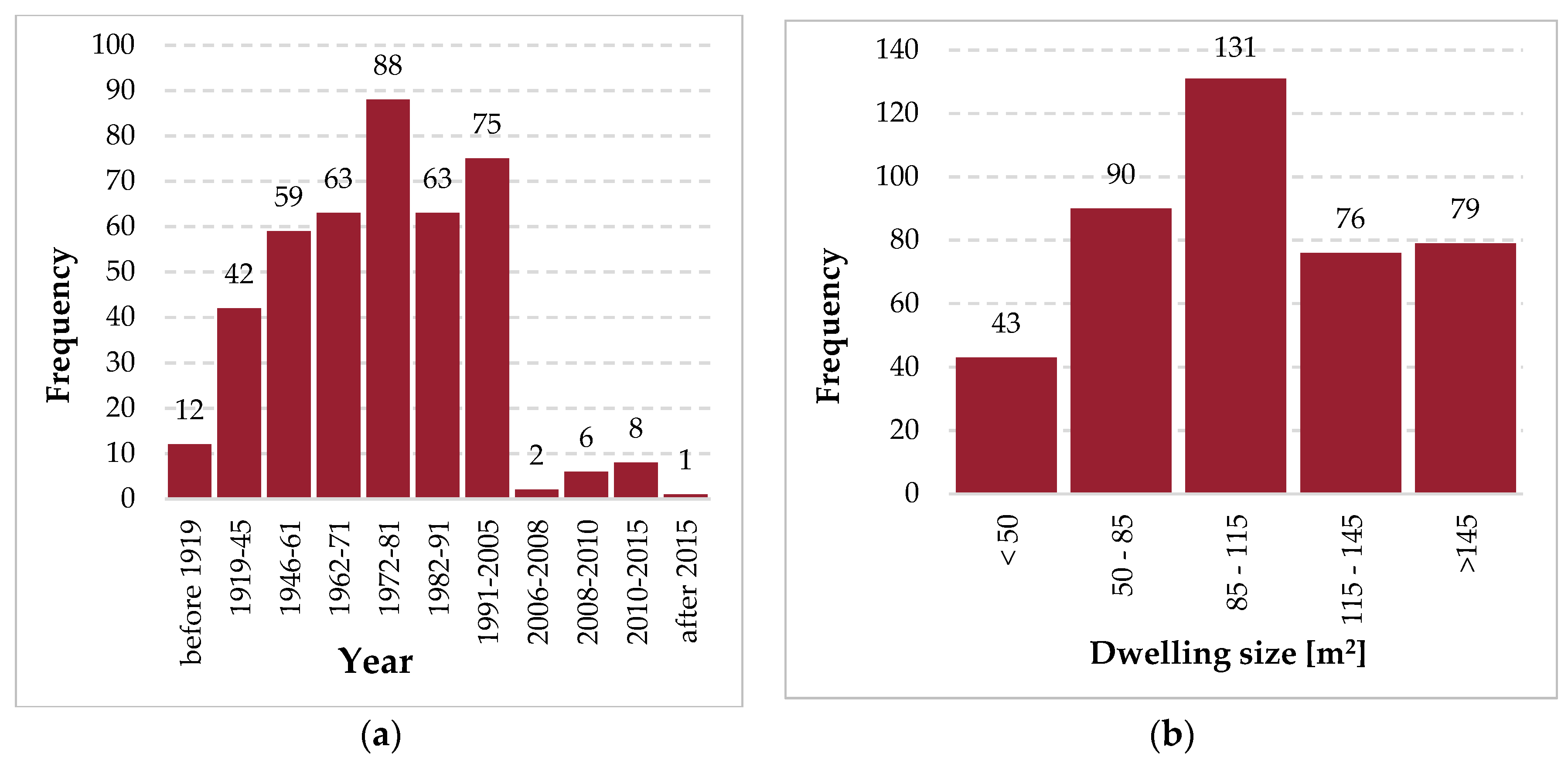
This section shows the analysis regarding frequency of the building main features. Figure 1a depicts the subdivision of the buildings according to the construction year, following the official classification used in the Italian population censuses [58]. A further division compared to the decades is done to account for law modifications in the field of building energy performance (years 2005, 2008, 2010, 2015). The data show that a wide part of the sample buildings belongs to before 1976, exactly the year of the first Italian law about energy saving.

Moreover, Figure 1b shows the building frequency related to their size according to their five different dimensional classes specifically: small <50 m²; small-medium 50–85 m²; medium 85–115 m²; medium-large 115–145 m²; large >145 m². The average size of the apartments is equal to 112.4 m² and the most common class is the medium one. These different sizes are connected to the family number of components the dwelling was designed for. It has to be pointed out that a great part of the considered dwellings occupy only one floor, i.e., 360 equal to 86.5% while, among the remaining ones 37, i.e., 8.9%, occupy two floors and 19, i.e., 4.6%, three floors.

The data acquisition procedure does not include the introduction of the characteristics of the walls by the user, but there is the indication concerning the construction year and any refurbishment carried out.

Table 4. Transmittance values depending on the construction year and the climate zone.

	Climate Zone	Construction Year
		Before 1919	1919–1945	1946–1961	1962–1971	1972–1981	1982–1991	1991–2005	2006–2008	2008–2010	2010–2015	After 2015
Walls	A	1.30	1.20	1.20	1.20	1.10	1.00	0.90	0.86	0.69	0.62	0.62
	B	1.30	1.20	1.20	1.20	1.07	1.00	0.87	0.67	0.53	0.48	0.48
	C	1.30	1.20	1.20	1.20	1.03	0.98	0.83	0.56	0.44	0.40	0.40
	D	1.30	1.20	1.20	1.20	1.00	1.00	0.80	0.50	0.40	0.36	0.36
	E	1.23	1.13	1.13	1.13	0.94	0.94	0.76	0.47	0.38	0.34	0.34
	F	1.19	1.10	1.10	1.10	0.92	0.92	0.73	0.46	0.37	0.33	0.33
Roofs	A	1.30	1.30	1.30	1.30	1.20	1.07	0.95	0.55	0.42	0.38	0.33
	B	1.30	1.30	1.30	1.30	1.17	1.01	0.90	0.55	0.42	0.38	0.33
	C	1.30	1.30	1.30	1.30	1.12	0.96	0.85	0.55	0.42	0.38	0.33
	D	1.30	1.30	1.30	1.30	1.10	0.90	0.80	0.46	0.35	0.32	0.28
	E	1.22	1.22	1.22	1.22	1.03	0.84	0.75	0.43	0.33	0.30	0.26
	F	1.18	1.18	1.18	1.18	1.00	0.82	0.73	0.42	0.32	0.29	0.25
Floors	A	1.10	1.20	1.20	1.20	1.10	1.08	1.08	0.83	0.74	0.65	0.65
	B	1.10	1.20	1.20	1.20	1.03	0.92	0.92	0.63	0.56	0.49	0.49
	C	1.10	1.20	1.20	1.20	0.96	0.80	0.80	0.54	0.48	0.42	0.42
	D	1.10	1.20	1.20	1.20	0.90	0.60	0.60	0.46	0.41	0.36	0.36
	E	1.01	1.10	1.10	1.10	0.83	0.55	0.55	0.42	0.38	0.33	0.33
	F	0.98	1.07	1.07	1.07	0.80	0.53	0.53	0.41	0.36	0.32	0.32
Windows	A	5.20	5.10	5.00	5.00	5.00	5.00	5.00	5.00	5.00	4.60	4.03
	B	5.20	5.10	5.00	5.00	5.00	5.00	4.33	3.88	3.50	3.00	2.63
	C	5.20	5.10	5.00	5.00	4.86	4.86	3.81	3.36	3.03	2.60	2.28
	D	5.20	5.10	5.00	5.00	5.00	5.00	3.00	3.10	2.80	2.40	2.10
	E	4.77	4.68	4.58	4.58	4.58	4.58	2.75	2.84	2.57	2.20	1.93
	F	4.33	4.25	4.17	4.17	4.17	4.17	2.50	2.58	2.33	2.00	1.75

shows the transmittance values of the buildings, depending on the construction year and according to the climate zone.

Reading the table, it is noteworthy that the current legislation provides a subdivision of the Italian territory into six climatic zones, according to the number of Degree Days (Zone A: DD ≤ 600; Zone B: 600 < DD ≤ 900; Zone C: 900 < DD ≤ 1400; Zone D: 1400 < DD ≤ 2100; Zone E: 2100 < DD ≤ 3000; Zone F: DD > 3000).

Table 5. Retrofitted building components.

Construction Year of the Building	Retrofitted Building Component
	Walls	Roofs	Floors	Windows
before 1919	0 (0%)	0 (0%)	0 (0%)	5 (41.7%)
1919–1945	2 (4.8%)	2 (4.8%)	3 (7.1%)	29 (69%)
1946–1961	6 (10.2%)	8 (13.6%)	1 (1.7%)	46 (78%)
1962–1971	8 (12.7%)	7 (11.1%)	3 (4.8%)	29 (46%)
1972–1981	13 (14.8%)	13 (14.8%)	5 (5.7%)	44 (50%)
1982–1991	6 (9.5%)	7 (11.1%)	4 (6.3%)	27 (42.9%)
1991–2005	16 (21.3%)	14 (18.7%)	9 (12%)	13 (17.3%)
2006–2008	0 (0%)	0 (0%)	0 (0%)	0 (0%)
2008–2010	2 (33.3%)	1 (16.7%)	0 (0%)	2 (33.3%)
2010–2015	4 (50%)	4 (50%)	3 (37.5%)	2 (25%)
after 2015	0 (0%)	0 (0%)	0 (0%)	0 (0%)
TOTAL	57 (13.6%)	56 (13.4%)	28 (6.7%)	197 (47%)

points out the number of dwellings that have undergone renovations, divided according to year of construction and type of intervention. The most frequent refurbishment intervention is the replacement of windows, carried out in 197 dwellings (47.0% of the total) [59]. Air leakage entailing heat losses and acoustic discomfort are the main reasons of such intervention [60]. For the new installed building components, a transmittance value was set equal to the most common of the same period of installation.

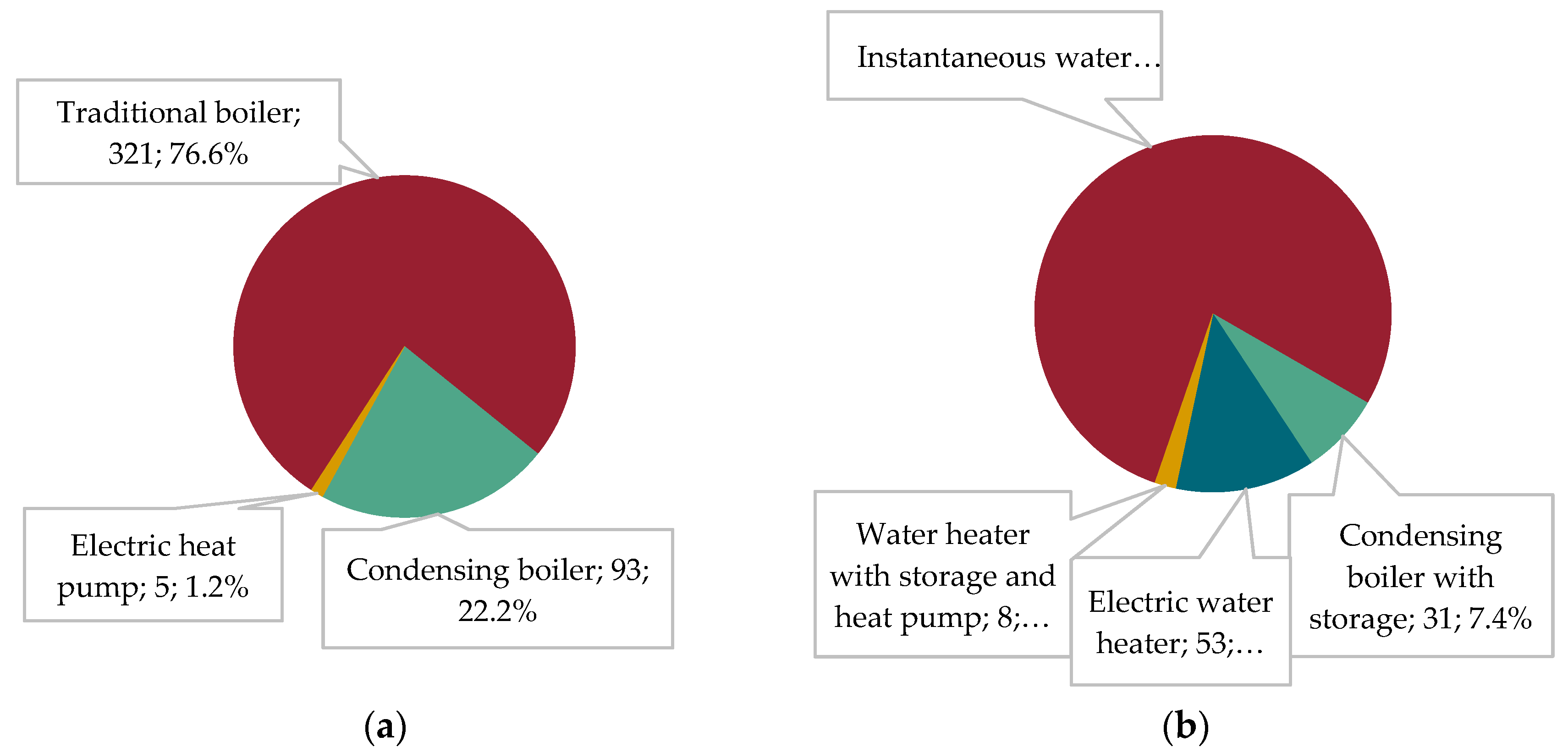
Regarding the HVAC systems, the analyzed dwellings are all equipped with a heating system and a DHW production system. Most of heating systems are autonomous (73.3%); gas is the most used energy vector in heating systems (98.8%) and in DHW preparation (85.4%). The majority of gas-fed systems provide both heating and DHW as shown in Figure 2.

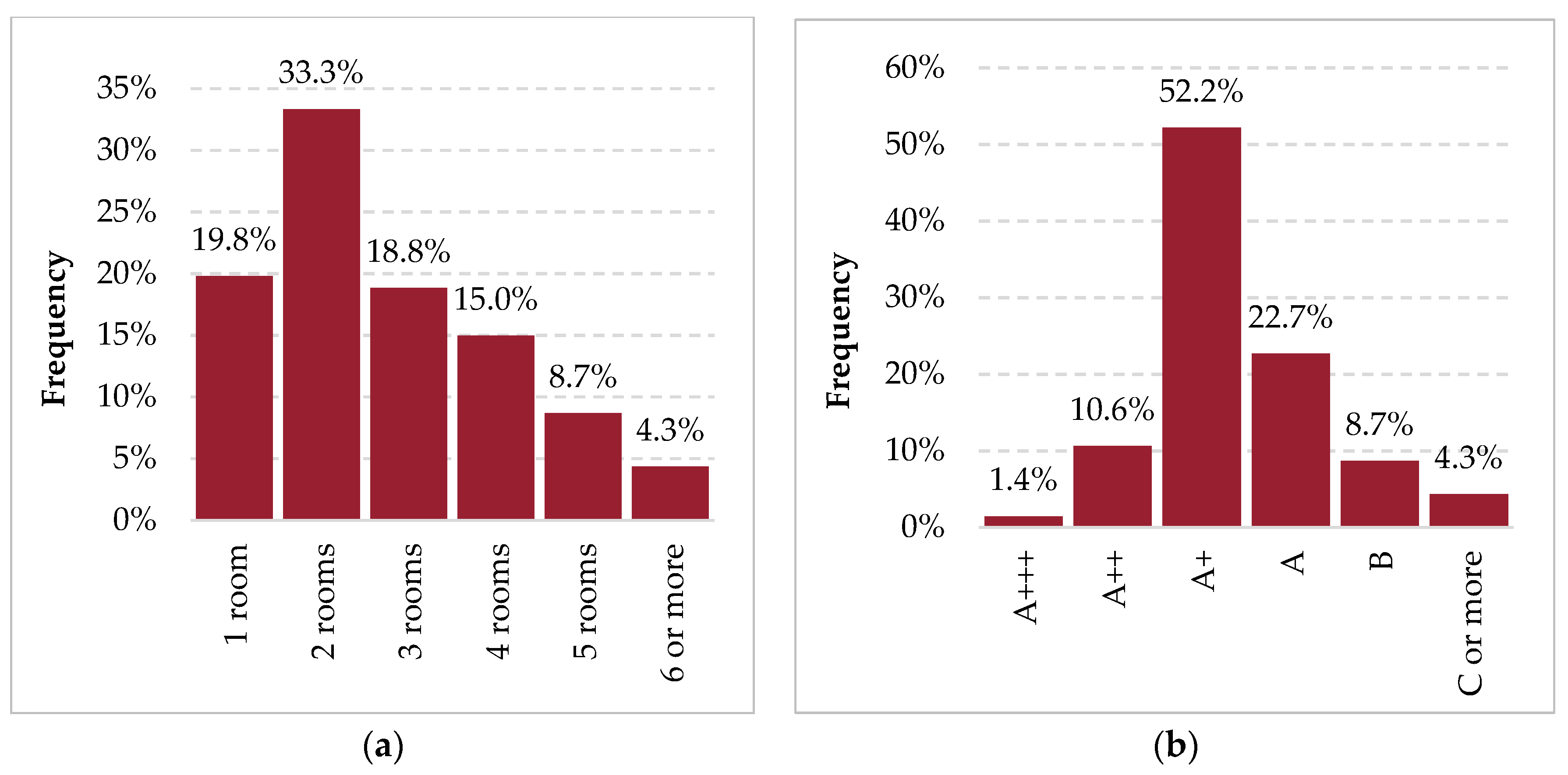
Cooling systems are installed only in 207 dwellings (49.4%). They serve only a few rooms, as depicted by Figure 3a and they show high energy label due to their very recent installation, as Figure 3b reports.

In order to validate the simulations’ outcomes from collected surveys, a comparison with energy bills was made. As a result of this comparison, a lower correlation between real and simulated gas consumption (R² = 0.7764) compared to the electricity one (R² = 0.8977) can be seen. The lower correlation relating to the use of gas depends on the greater uncertainty of occupants’ profiles in dwellings and high incidence of this service on energy consumption.

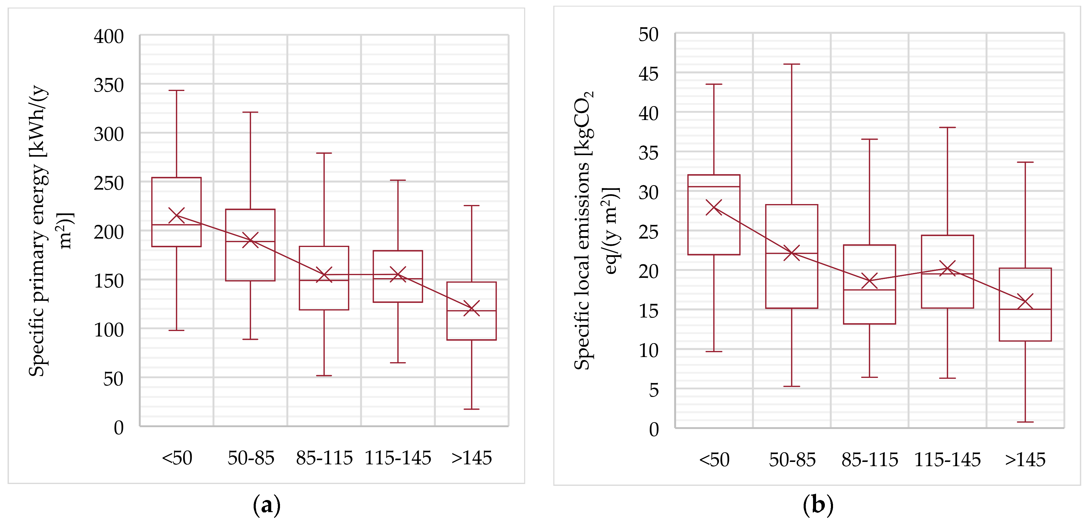
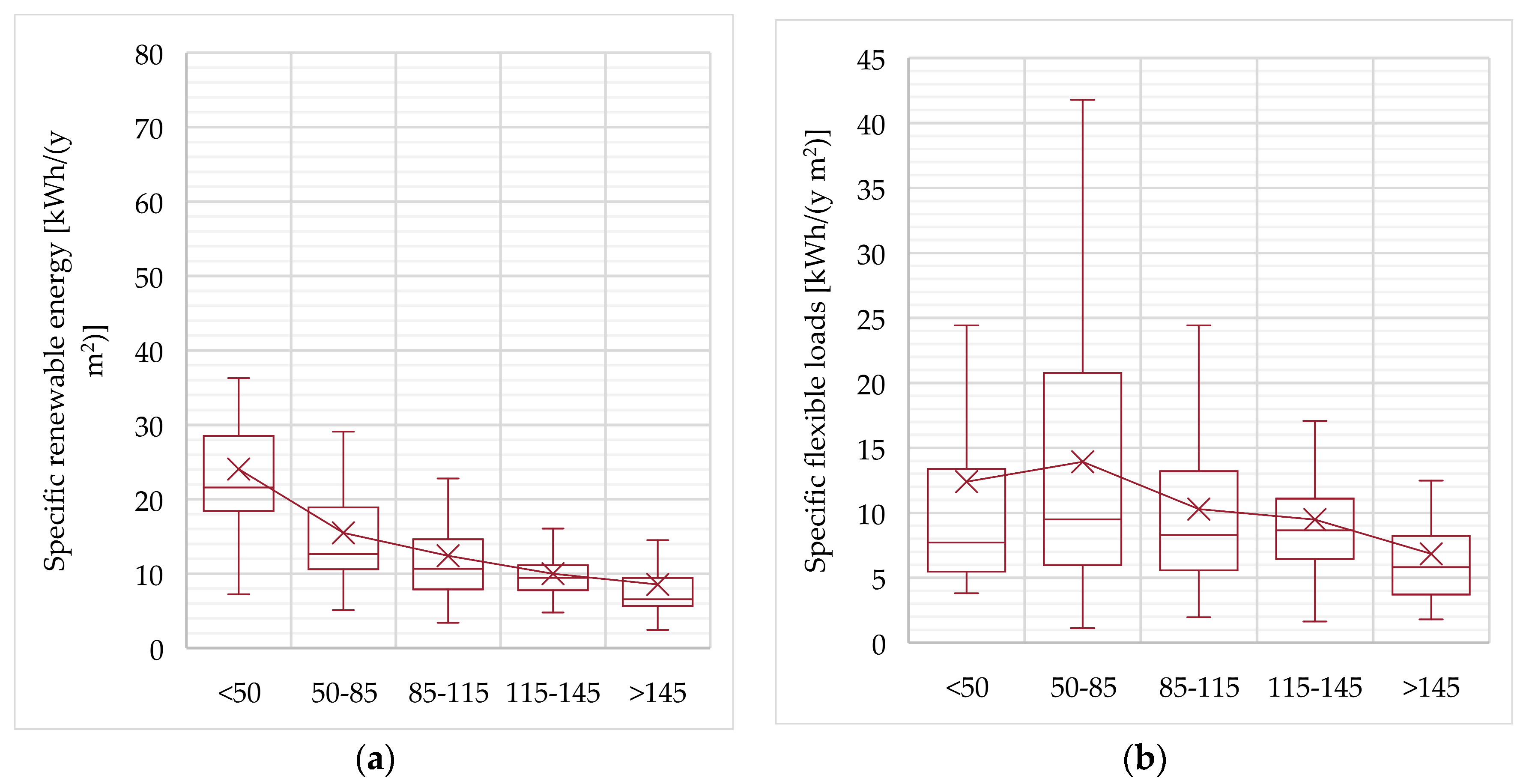
The charts of Figure 4 and Figure 5 show a calculation per unit of surface of the selected indicators: (i) primary energy consumption, (ii) local emissions, (iii) use of renewable energy, and (iv) flexible loads per class of sizes.

At apartment size increases, the average value of primary energy consumption per unit of area decreases, from 215.0 kWh/m²y (small dwelling) to 120.6 kWh/m²y (large dwelling). Even the local emissions, in terms of equivalent CO₂, show a decreasing trend from 27.9 kg/m²y (small dwelling) to 16.1 kg/m²y (large dwelling). This is due to the lower ratio between surface and volume in the largest dwelling as well as lower specific occupancy rate. Regarding the medium-large dwellings, a slight variation due to the higher incidence of gas consumption for heating on the overall energy one is found. The larger houses with greater frequency are isolated. They have larger dispersing surfaces and, subsequently, heat losses [61].

Similarly, in Figure 5a, renewable energy consumption per unit of area decreases as the size of the apartment increases, from 24.1 kWh/m²y (small dwelling) to 8.5 kWh/m²y (large dwelling).

The consideration of another parameter is remarkable: the electrification degree. It is the ratio between the electricity consumption and the total primary energy one. It is on average 36.3% for the considered building stock. Next, the consumption of renewable energy is on average equal to 9.0%, depending largely on the renewable share of the power grid where they buy electricity from.

Even for flexible loads per unit of area, a decreasing trend is observed at increasing the dwelling surface, although not continuous, from 12.4 kWh/m²y (small dwelling) to 6.9 kWh/m²y (large dwelling). This is due the fact that different occupancy profiles occur since the small ones have higher rate of occupants’ absence compared to the large one. In absolute terms, average flexible electric loads of the analyzed dwellings [54] are equal to 1043 kWh/y and they are largely shiftable loads (667 kWh/y) related to the use of washing machines, dishwashers, and dryers. Storable loads have a lower average magnitude (376 kWh/y), due to the low diffusion of electric heating and DHW systems and as a consequence of the low presence of cooling systems.

3.2. Building Envelope Retrofitting Measures

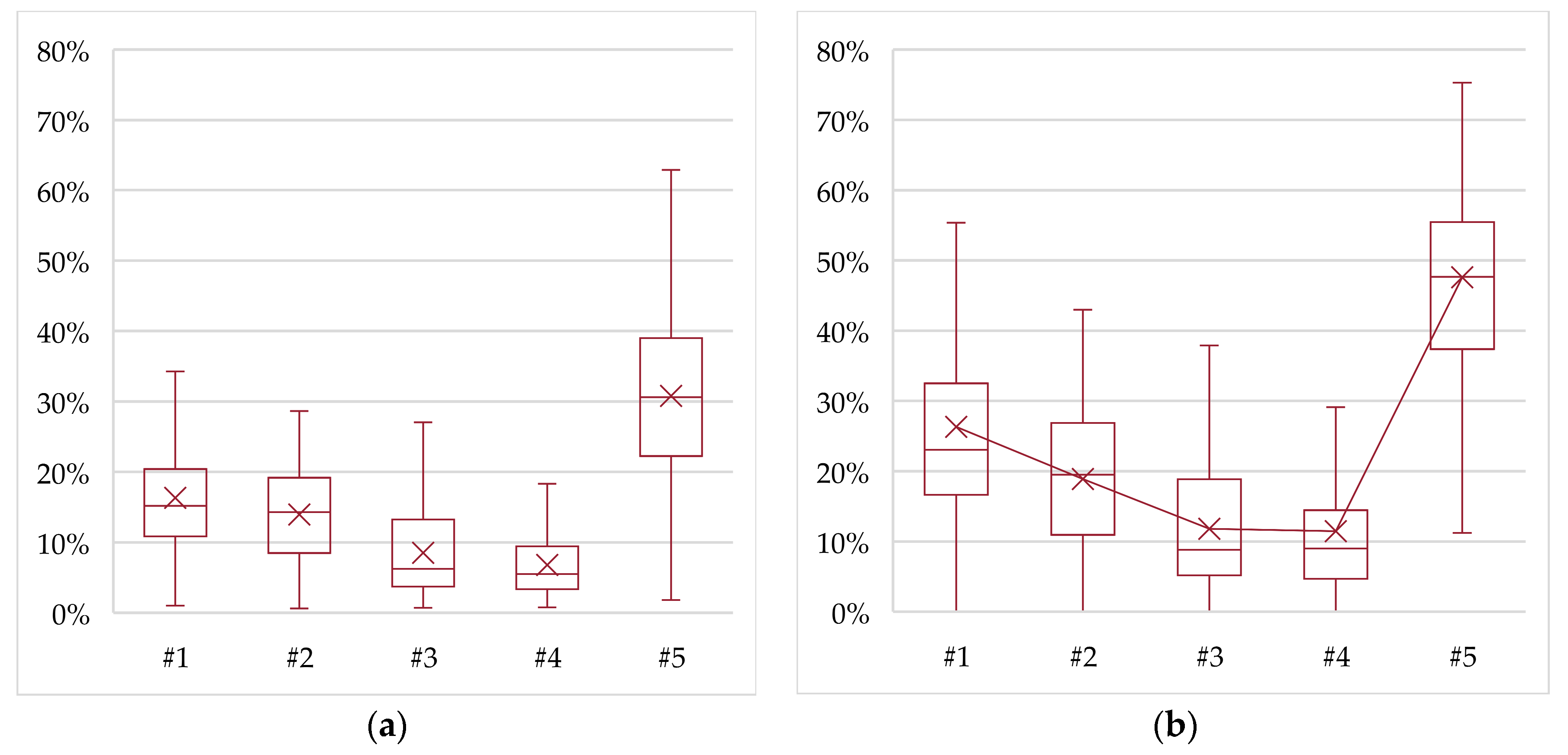
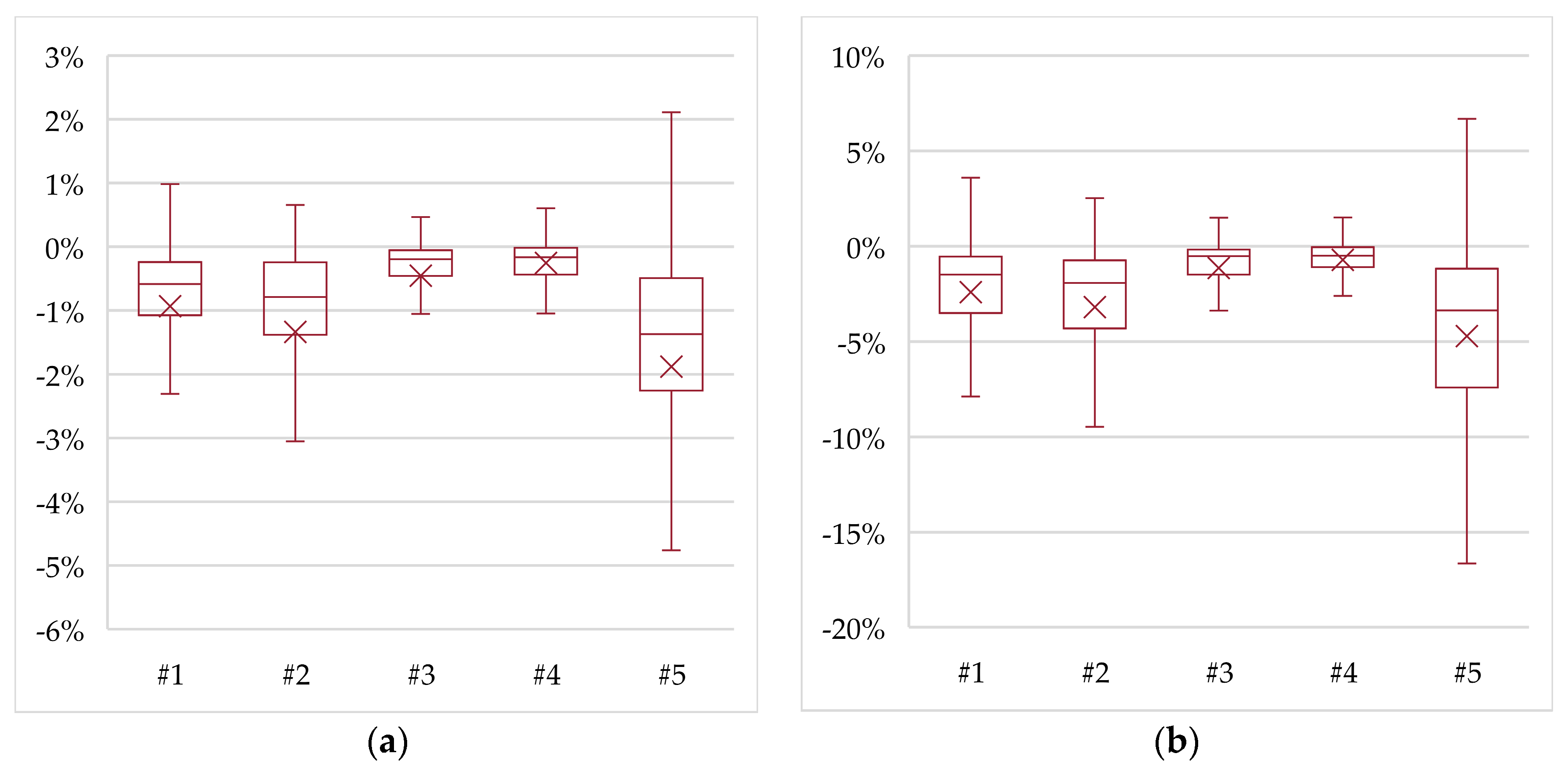
In all the retrofitting cases a reduction in heating and cooling consumption occurs. Its magnitude is linked to the relevance of the retrofitted building component on the energy consumption of the examined house, depending on the single case’s geometric and thermo-physical parameters. Figure 6 shows the primary energy savings and the reduction of local emissions compared to the current situation. Evaluating the single interventions, the largest primary energy savings are linked to the interventions of isolation on the vertical opaque walls, on average equal to 16.3%, while, the smallest savings derive from the window ones, about 6.8%. This is due to the fact that, in many dwellings, the windows have been recently replaced. The intervention of insulation on ceilings and floors allows on average savings of 14.0% and 8.5%, respectively. However, the retrofitting of the whole building envelope can lead to a primary energy saving of about 30.8%. The trend of savings in local emissions is qualitatively similar to the primary energy one, although amplified: for vertical opaque walls a saving of 26.3% is achievable; for ceilings, 18.9%; for floors, 11.8%, and for fixtures, 11.5%. It leads to on average 47.6% in the case of the whole retrofitted building envelope. The reason for this amplification lies in the fact that, as seen, most of the heating systems are gas-fired and require local combustion to generate heat.

Figure 7 shows the variations in the use of renewable energy and the number of flexible loads at each retrofitted building component.

The considered insulation interventions lead to a reduction in heating and cooling consumption, i.e., storable loads.

Moreover, the small variations are connected to the reduction of the electric consumption of the components of the heating system such as circulation pumps and fans, and to the reduction of cooling consumption, in the houses, if present.

Considering the whole building insulation intervention, the reduction of renewable energy use is less than 2% and the reduction of flexible loads is less than 5%.

Indeed, in the current plant configuration of Italian houses, a redevelopment intervention of the building envelope weakly affects the flexibility potential of the house. Yet, it entails valuable energy savings and reductions in local polluting emissions. In absolute terms, in the case of the whole building envelope retrofitting, flexible loads vary from 1043 to 1002 kWh/y.

3.3. Heating, Cooling, and DHW Systems Upgrading

In all the upgrading cases, a reduction in heating and cooling consumption occurs. Its magnitude is related to the relevance of the redeveloped element on the energy consumption of the analyzed dwelling, depending on the single case geometric and thermo-physical parameters.

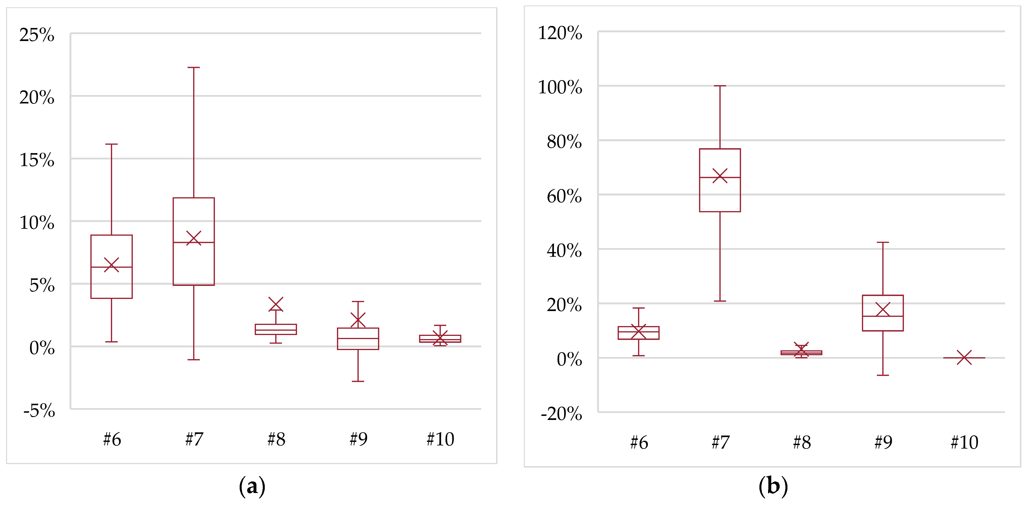
Figure 8 shows the primary energy savings and the reduction of local emissions compared to the current situation. The largest savings in primary energy are observed for interventions on the heating system’s heat generator, due to the high incidence of heating consumption on overall consumption [54]. For the upgrade option #6 the savings are on average equal to 6.5%, while for upgrade option #7 they are on average equal to 8.6%. Almost negligible savings, i.e., <1.5%, in all the other upgrading options occur.

Referring to the local emissions, the achievable reduction due to the installation of a heat pump as a heat generator and as the DHW production system are huge since they are 66.9% and 17.8%, respectively.

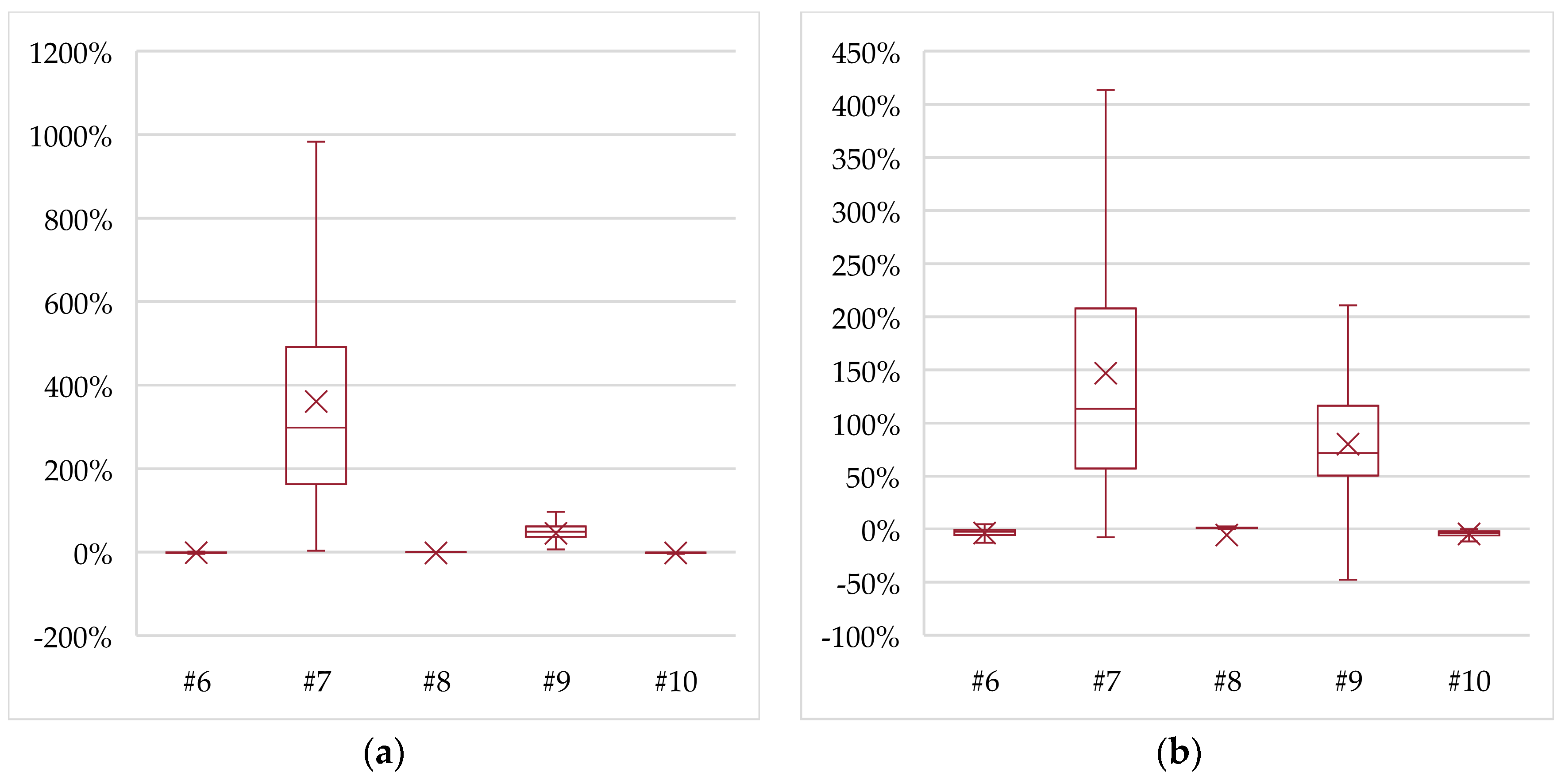
Figure 9 shows the variations in the renewable energy use and the number of flexible loads at each system upgrade. Similar to the previous KPIs, the changes in those two thanks to the installation of heat pump are very significant (#7, #9). For the system upgrading #7, the increase in renewable energy use is on average 360% while, for the system upgrading #9, the variation is 45.4%. It is remarkable that for the other system upgrading the changes are very small: −1.2%, −2.1%, and −1.7% for #6, #8, and #10, respectively. The same behavior can be found for the changes in flexible loads. Indeed, system upgrading #7 and #9 imply their significant increases, about 147.0% and 80.1%, respectively. Then, small decreases occur for system upgrading #6, #8, and #10, i.e., −3.8%, −5.7%, and −4.8%. In absolute terms, the flexible loads in the system upgrading #7 reach 2111 kWh/y, whereas in #9, they reach 1443 kWh/y.

The results of the simulations carried out confirm the usefulness of the heat pumps to increase the flexibility of the loads [62,63], as a basic element of a system that must necessarily include storage systems [64,65,66]. Anyway, the location of the storage system inside the dwellings remains to be explored. As a matter of fact, the DHW storage system is generally small [23] and easy to install inside the dwelling. Nevertheless, the storage system required for space heating is much larger, depending on the climate zone, the characteristics of the house, and the behavior of the occupants [67] together with needed preservation of architectural appearance when the building is considered historic or even listed [68].

3.4. Combined Building Envelope Retrofitting and System Upgrading

Finally, given the small changes observed in the previous section, the intervention to upgrade the cooling system was excluded.

Figure 10 shows the primary energy savings and the reduction of local emissions compared to the current situation. In terms of primary energy savings, the five combined scenarios are substantially equivalent, with savings ranging between 32.6%, in the case of #11, and 35.7%, in the case of #14.

Referring to local emissions, the achievable reductions are larger than 50% for all the combined scenarios, being able to reach 84.9% in the case of scenario #15, i.e., with complete electrification of space heating and DHW production.

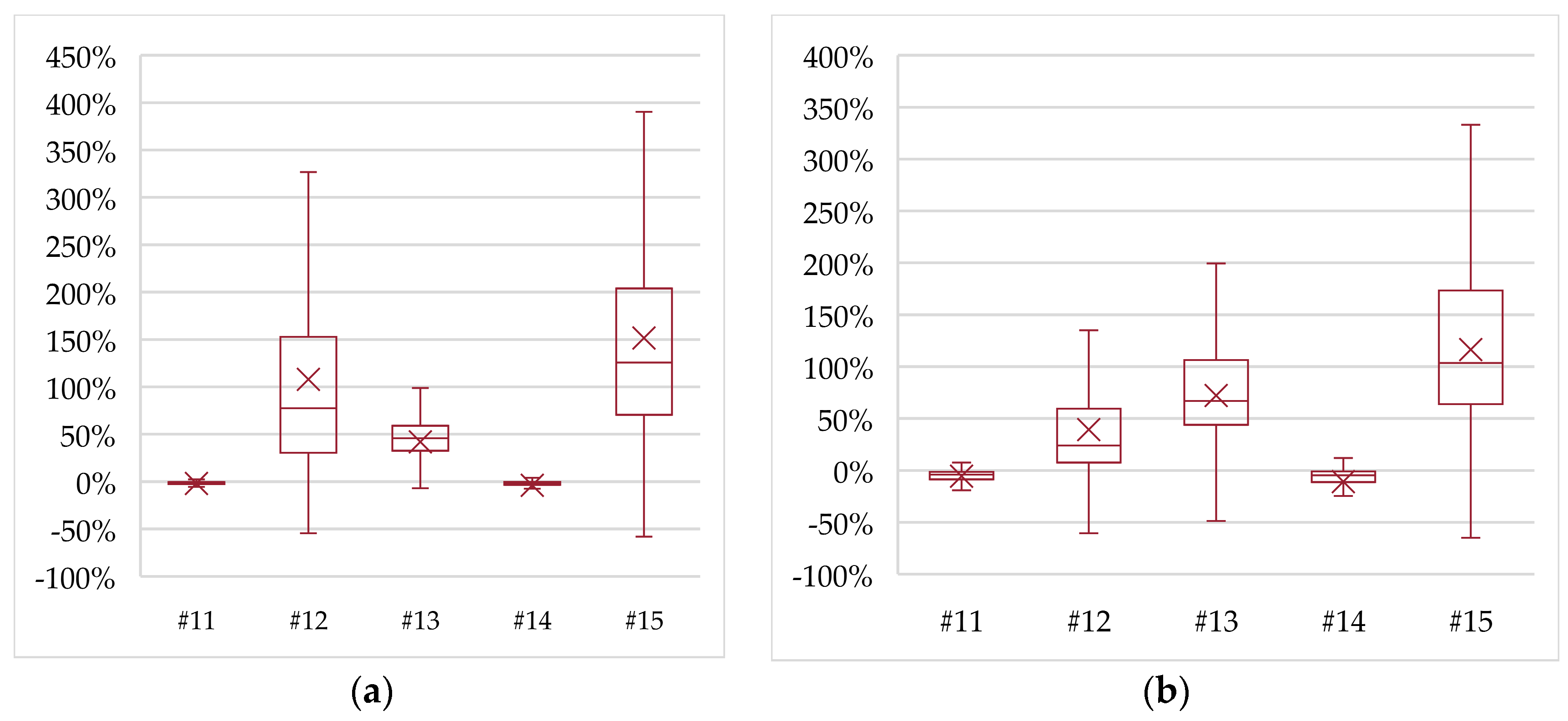
Figure 11 shows the variations in the renewable energy use and the number of flexible loads at each combined retrofitting and system upgrading. As the outcome of system upgrading scenarios, the introduction of the heat pump as a heat generator significantly increase the renewable energy use, reaching on average values greater than 150% as in the case #15. Even in terms of flexible electric loads, a strong increase in the flexibility potential occurs, reaching 116.4% in the case of #15.

In absolute terms, the value of flexible loads in scenarios #12, #13, and #15 reaches 1.329, 1.399, and 1.725 kWh/y, respectively.

These results are numerically lower than those found for scenario #7 where there was the installation of the single heat pump for space heating purposes. However, in this case, the lower increase in flexibility potential matches with positive values of all the other KPIs, i.e., primary energy savings, local emission reduction, and renewable energy use. Furthermore, the reduction of the heating demand has as a further positive aspect, an easier insertion of the storage system within the dwelling due to its new smaller required size [67].

3.5. Effects of the Proposed Measures

The changes deriving from the implementation of renovation measures are summarized in

Table 6. Summary of interventions and related changes.

		Resulted Savings		Resulted Changes
#	Intervention	Primary Energy Consumption	Local Emissions	Renewable Energy Use	Flexible Loads
#1	Vertical opaque walls	16.3%	26.3%	−0.9%	−2.4%
#2	Roof covering	14.0%	18.9%	−1.3%	−3.2%
#3	Lower floor	8.5%	11.8%	−0.5%	−1.1%
#4	Windows	6.8%	11.5%	−0.3%	−0.7%
#5	Global upgrading of the envelope	30.8%	47.6%	−1.9%	−4.7%
#6	Heating	6.5%	9.7%	−1.2%	−3.8%
#7	Heating—HP	8.6%	66.9%	360.8%	147.0%
#8	DHW	3.4%	3.2%	−2.1%	−5.7%
#9	DHW—HP	2.1%	17.8%	45.4%	80.1%
#10	Cooling	0.7%	0.1%	−1.7%	−4.8%
#11	Overall envelope + heating system	32.6%	50.3%	−2.1%	−5.5%
#12	Overall envelope + heating system HP	33.2%	67.4%	107.9%	39.4%
#13	Overall envelope + DHW HP	32.8%	64.8%	41.9%	72.2%
#14	Overall envelope + heating + DHW	35.7%	53.1%	−3.9%	−10.8%
#15	Overall envelope + heating HP + DHW HP	35.5%	84.9%	151.6%	116.4%

reporting the values computed of the four KPIs.

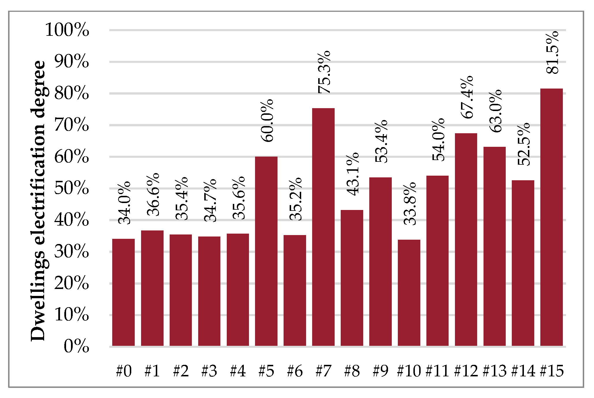
Figure 12 depicts the electrification degree resulting from the 15 proposed interventions and combinations of them. In the status quo, the average electrification degree, i.e., the ratio between electrical loads and total ones, is 34%. Conversely, the highest value is reached in all the interventions apart from #10 which is 33.8% since the electric loads are reduced making the cooling supply more efficient. Interventions #5, #11, and #14 increase the mentioned parameter thanks the high reduction of heating consumption while interventions #7, #9, #12, #13, and #15 achieved the highest values switching the heating from fossil-based to electric-driven.

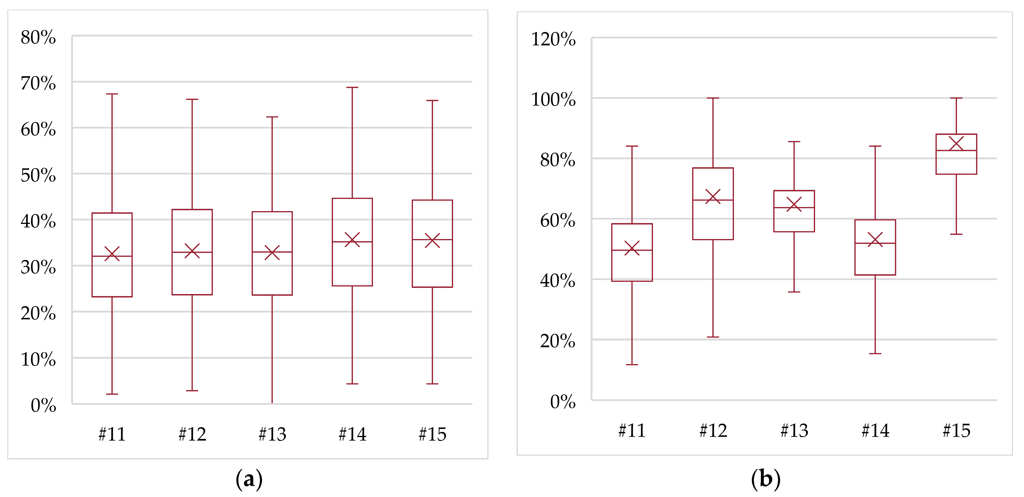
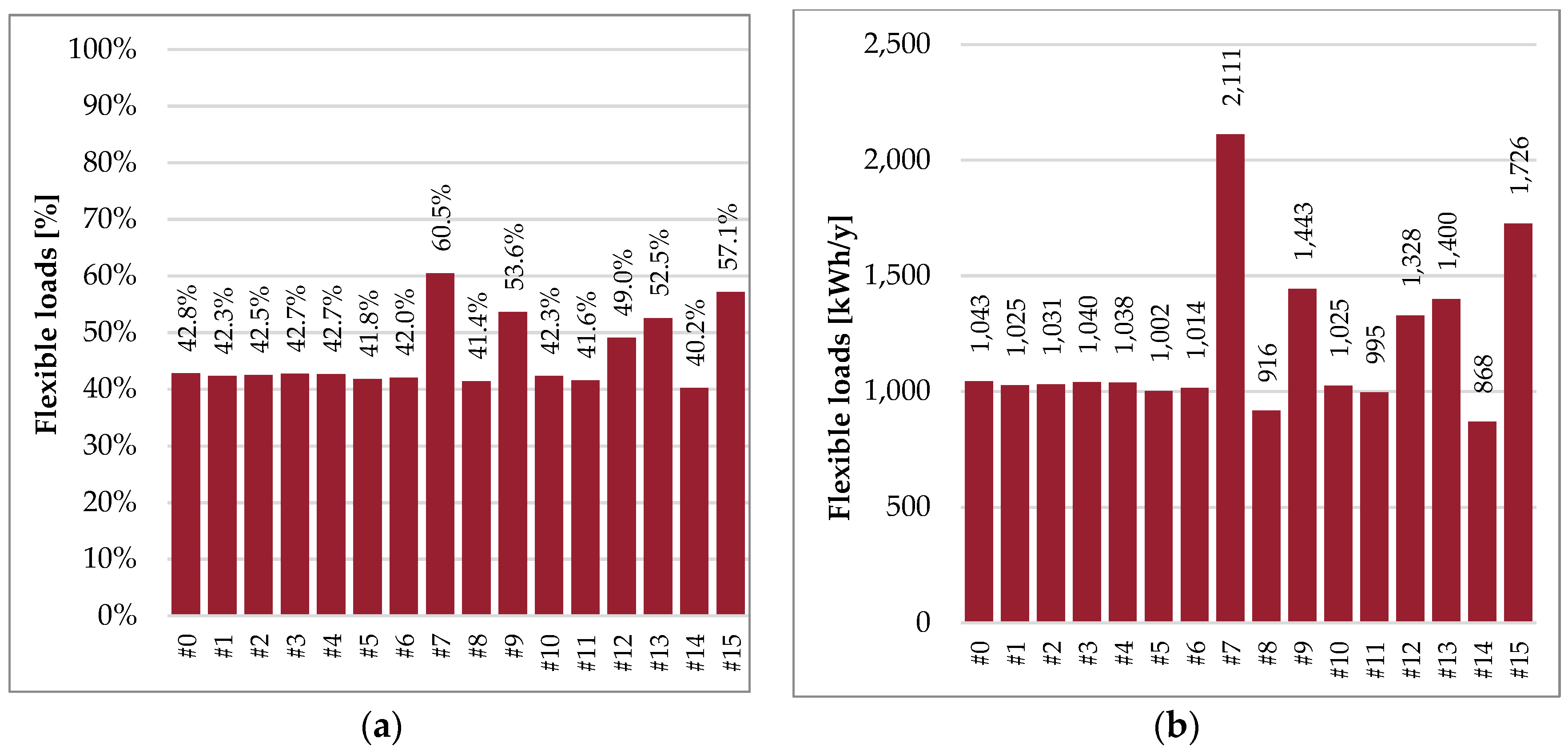
Figure 13a shows the flexible loads in percentage value in part while, in absolute values in Figure 13b. Strong changes are found only for the electrification of the heating systems by means of heat pumps for heating and/or for DHW. Those interventions are #7, #9, #12, #13, and #15.

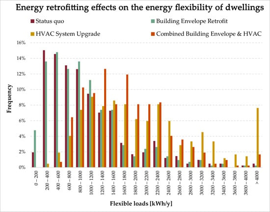
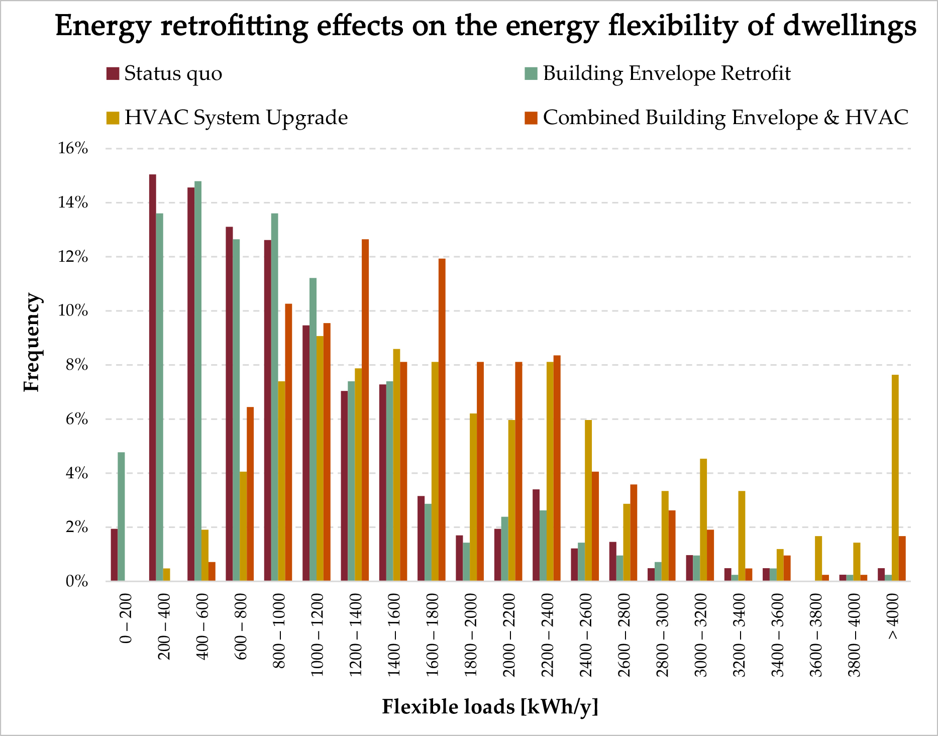
Finally Figure 14a depicts how the frequency of flexible loads is before the intervention #0, and in Figure 14b after the comprehensive renovation #15. In the latter, 40% of dwellings show flexible loads lower than 1400 kWh/y. If the value 1800 kWh/y is considered, 60% of the analyzed residential building stock is under it. Only 32.2% of dwellings have more than 2000 kWh/y flexible loads.

4. Conclusions

The European community has outlined its objectives in the field of environmental sustainability, indicating ambitious targets for reducing energy consumption, reducing emissions, and increasing the use of renewable energy sources. In this context, the study of energy retrofitting of existing buildings is of fundamental importance, as the building sector is responsible for more than 40% of total consumption. These interventions must be inserted in a new energy scenario, in which greater electrification of consumption and greater flexibility of demand will allow a wider integration of renewable energies. In this study, referring to the Italian situation, energy retrofitting interventions for the residential sector were analyzed, using a set of four Key Performance Indicators, i.e., primary energy consumption, renewable energy use, local polluting emissions, and flexible electrical loads. The interventions here analyzed are on the building envelope, on systems upgrading and, finally, a combination of them.

Considering the current situation, it was observed that:

• the Italian residential sector is not endowed with enough electrification; gas is the most widely used energy vector for space heating (98.8%) and DHW production (85.4%);
• only 49.4% of the dwellings surveyed are equipped with cooling systems;
• as the size of the apartment increases, primary energy consumption per unit area decreases; a similar trend is seen in the renewable energy use and local polluting emissions;
• for flexible loads per unit area, an overall decreasing trend occurs but with the exception of small-medium dwellings (50–85 m²).
• As for the energy retrofitting interventions on the building envelope, it was observed that:
• all interventions involve a reduction in energy consumption and a reduction in polluting emissions;
• all the considered interventions involve a reduction in renewable energy use and a decrease in flexible loads.

With regard to the system upgrading, a clear difference was observed between gas-fed systems for space heating and DHW and electrified services by means of heat pump installation. In this case, a considerable increase in flexible loads and the renewable energy use occur with a strong reduction in local emissions due the increase of the power grid supply.

The results of the simulations carried out to evaluate the effects of a combined building envelope and system improvement are as summarized below:

• all combined interventions imply a reduction of primary energy consumption;
• a correlated reduction of local polluting emissions is found for gas-fed condensing boiler installation, while there are higher values of reduced local emissions in the case of electrification of space heating and DHW by means of heat pumps;
• all combined interventions entail a larger renewable energy use and a larger flexibility if heat pumps are to be installed;
• a total of 50% of the renovated dwellings in the #15 scenario show a flexibility between 1200 and 2400 kWh/y entailing the possibility to use it as a reference value for preliminary calculation of aggregated users.

It is noteworthy how the results of this study can offer a further KPI to evaluate the best retrofitting intervention, from an economic perspective, accounting for new electricity business models in the era of prosumers where flexibility is becoming the new performance of the built environment.

References

- European Commission. A Clean Planet for All—A European Strategic Long-Term Vision for a Prosperous, Modern, Competitive and Climate Neutral Economy; European Commission: Brussels, Belgium, 2018. [Google Scholar]
- Eurostat Database—Eurostat. Available online: https://ec.europa.eu/eurostat/data/database (accessed on 4 April 2019).
- Piras, G.; Pini, F.; Garcia, D.A. Correlations of PM10 concentrations in urban areas with vehicle fleet development, rain precipitation and diesel fuel sales. Atmospheric Pollut. Res. 2019, 10, 1165–1179. [Google Scholar] [CrossRef]
- Aste, N.; Manfren, M.; Marenzi, G. Building Automation and Control Systems and performance optimization: A framework for analysis. Renew. Sustain. Energy Rev. 2017, 75, 313–330. [Google Scholar] [CrossRef]
- Nezhad, M.M.; Groppi, D.; Rosa, F.; Piras, G.; Cumo, F.; Garcia, D.A. Nearshore wave energy converters comparison and Mediterranean small island grid integration. Sustain. Energy Technol. Assess. 2018, 30, 68–76. [Google Scholar]
- Tronchin, L.; Manfren, M.; Nastasi, B. Energy analytics for supporting built environment decarbonisation. Energy Procedia 2019, 157, 1486–1493. [Google Scholar] [CrossRef]
- Nastasi, B. “Hydrogen Policy, Market and R&D Projects” in Solar Hydrogen Production; Calise, F., D’Accadia, M.D., Santarelli, M., Lanzini, A., Ferrero, D., Eds.; Elsevier: Amsterdam, The Netherlands, 2019; ISBN 9780128148532. [Google Scholar]
- Zappa, W.; Junginger, M.; van den Broek, M. Is a 100% renewable European power system feasible by 2050? Appl. Energy 2019, 233–234, 1027–1050. [Google Scholar] [CrossRef]
- De Santoli, L.; Mancini, F.; Garcia, D.A. A GIS-based model to assess electric energy consumptions and usable renewable energy potential in Lazio region at municipality scale. Sustain. Cities Soc. 2019, 46, 101413. [Google Scholar] [CrossRef]
- Adhikari, R.; Aste, N.; Manfren, M.; Adhikari, R. Multi-commodity network flow models for dynamic energy management—Smart Grid applications. Energy Procedia 2012, 14, 1374–1379. [Google Scholar] [CrossRef]
- Hossain, M.; Madlool, N.; Rahim, N.; Selvaraj, J.; Pandey, A.; Khan, A.F. Role of smart grid in renewable energy: An overview. Renew. Sustain. Energy Rev. 2016, 60, 1168–1184. [Google Scholar] [CrossRef]
- Rahmani-Andebili, M. Modeling nonlinear incentive-based and price-based demand response programs and implementing on real power markets. Electr. Power Syst. Res. 2016, 132, 115–124. [Google Scholar] [CrossRef]
- Aghajani, G.; Shayanfar, H.; Shayeghi, H. Demand side management in a smart micro-grid in the presence of renewable generation and demand response. Energy 2017, 126, 622–637. [Google Scholar] [CrossRef]
- Tronchin, L.; Manfren, M.; James, P.A. Linking design and operation performance analysis through model calibration: Parametric assessment on a Passive House building. Energy 2018, 165, 26–40. [Google Scholar] [CrossRef] [Green Version]
- De Santoli, L.; Garcia, D.A.; Groppi, D.; Bellia, L.; Palella, B.I.; Riccio, G.; Cuccurullo, G.; Ambrosio, F.R.D.; Stabile, L.; Dell’Isola, M.; et al. A General Approach for Retrofit of Existing Buildings Towards NZEB: The Windows Retrofit Effects on Indoor Air Quality and the Use of Low Temperature District Heating. In Proceedings of the 2018 IEEE International Conference on Environment and Electrical Engineering and 2018 IEEE Industrial and Commercial Power Systems Europe (EEEIC/I&CPS Europe), Palermo, Italy, 12–15 June 2018; pp. 1–6. [Google Scholar]
- Castellani, B.; Morini, E.; Nastasi, B.; Nicolini, A.; Rossi, F. Small-Scale Compressed Air Energy Storage Application for Renewable Energy Integration in a Listed Building. Energies 2018, 11, 1921. [Google Scholar] [CrossRef]
- Bartusch, C.; Wallin, F.; Odlare, M.; Vassileva, I.; Wester, L. Introducing a demand-based electricity distribution tariff in the residential sector: Demand response and customer perception. Energy Policy 2011, 39, 5008–5025. [Google Scholar] [CrossRef]
- Wang, J.; Li, P.; Fang, K.; Zhou, Y. Robust Optimization for Household Load Scheduling with Uncertain Parameters. Appl. Sci. 2018, 8, 575. [Google Scholar] [CrossRef]
- Koch, A.; Girard, S.; McKoen, K. Towards a neighbourhood scale for low- or zero-carbon building projects. Build. Res. Inf. 2012, 40, 527–537. [Google Scholar] [CrossRef]
- Corbin, C.D.; Henze, G.P. Predictive control of residential HVAC and its impact on the grid. Part II: simulation studies of residential HVAC as a supply following resource. J. Build. Perform. Simul. 2017, 10, 365–377. [Google Scholar] [CrossRef]
- Li, W.; Yang, L.; Ji, Y.; Xu, P. Estimating demand response potential under coupled thermal inertia of building and air-conditioning system. Energy Build. 2019, 182, 19–29. [Google Scholar] [CrossRef]
- Foteinaki, K.; Li, R.; Heller, A.; Rode, C. Heating system energy flexibility of low-energy residential buildings. Energy Build. 2018, 180, 95–108. [Google Scholar] [CrossRef]
- Balint, A.; Kazmi, H. Determinants of energy flexibility in residential hot water systems. Energy Build. 2019, 286–296. [Google Scholar] [CrossRef]
- Issi, F.; Kaplan, O. The Determination of Load Profiles and Power Consumptions of Home Appliances. Energies 2018, 11, 607. [Google Scholar] [CrossRef]
- Ruzzenenti, F.; Bertoldi, P. Energy Conservation Policies in the Light of the Energetics of Evolution; Springer Science and Business Media LLC: Berlin/Heidelberg, Germany, 2017; Volume 493, pp. 147–167. [Google Scholar]
- Tzeiranaki, S.T.; Bertoldi, P.; Diluiso, F.; Castellazzi, L.; Economidou, M.; Labanca, N.; Serrenho, T.R.; Zangheri, P. Analysis of the EU Residential Energy Consumption: Trends and Determinants. Energies 2019, 12, 1065. [Google Scholar] [CrossRef]
- Wang, B.; Xia, X.; Zhang, J. A multi-objective optimization model for the life-cycle cost analysis and retrofitting planning of buildings. Energy Build. 2014, 77, 227–235. [Google Scholar] [CrossRef] [Green Version]
- Fan, Y.; Xia, X. A multi-objective optimization model for energy-efficiency building envelope retrofitting plan with rooftop PV system installation and maintenance. Appl. Energy 2017, 189, 327–335. [Google Scholar] [CrossRef] [Green Version]
- Wu, R.; Mavromatidis, G.; Orehounig, K.; Carmeliet, J. Multiobjective optimisation of energy systems and building envelope retrofit in a residential community. Appl. Energy 2017, 190, 634–649. [Google Scholar] [CrossRef]
- Penna, P.; Prada, A.; Cappelletti, F.; Gasparella, A. Multi-objectives optimization of Energy Efficiency Measures in existing buildings. Energy Build. 2015, 95, 57–69. [Google Scholar] [CrossRef]
- Asadi, E.; Da Silva, M.G.; Antunes, C.H.; Dias, L.; Da Silva, M.C.G. Multi-objective optimization for building retrofit strategies: A model and an application. Energy Build. 2012, 44, 81–87. [Google Scholar] [CrossRef]
- Guardigli, L.; Bragadin, M.A.; Della Fornace, F.; Mazzoli, C.; Prati, D. Energy retrofit alternatives and cost-optimal analysis for large public housing stocks. Energy Build. 2018, 166, 48–59. [Google Scholar] [CrossRef]
- Dall’O’, G.; Galante, A.; Pasetti, G. A methodology for evaluating the potential energy savings of retrofitting residential building stocks. Sustain. Cities Soc. 2012, 4, 12–21. [Google Scholar] [CrossRef]
- De Santoli, L.; Mancini, F.; Nastasi, B.; Ridolfi, S. Energy retrofitting of dwellings from the 40’s in Borgata Trullo-Rome. Energy Procedia 2017, 133, 281–289. [Google Scholar] [CrossRef]
- Mancini, F.; Salvo, S.; Piacentini, V. Issues of Energy Retrofitting of a Modern Public Housing Estates: The ‘Giorgio Morandi’ Complex at Tor Sapienza, Rome, 1975–1979. Energy Procedia 2016, 101, 1111–1118. [Google Scholar] [CrossRef]
- Niemelä, T.; Kosonen, R.; Jokisalo, J. Energy performance and environmental impact analysis of cost-optimal renovation solutions of large panel apartment buildings in Finland. Sustain. Cities Soc. 2017, 32, 9–30. [Google Scholar] [CrossRef] [Green Version]
- Ortiz, J.I.; Casas, A.F.; Salom, J.; Soriano, N.G.; Casas, P.F.I.; Ferrà, J.A.O. Cost-effective analysis for selecting energy efficiency measures for refurbishment of residential buildings in Catalonia. Energy Build. 2016, 128, 442–457. [Google Scholar] [CrossRef] [Green Version]
- Valančius, K.; Vilutienė, T.; Rogoža, A. Analysis of the payback of primary energy and CO2 emissions in relation to the increase of thermal resistance of a building. Energy Build. 2018, 179, 39–48. [Google Scholar] [CrossRef]
- Mancini, F.; Cecconi, M.; De Sanctis, F.; Beltotto, A. Energy Retrofit of a Historic Building Using Simplified Dynamic Energy Modeling. Energy Procedia 2016, 101, 1119–1126. [Google Scholar] [CrossRef]
- De Santoli, L.; Mancini, F.; Clemente, C.; Lucci, S. Energy and technological refurbishment of the School of Architecture Valle Giulia, Rome. Energy Procedia 2017, 133, 382–391. [Google Scholar] [CrossRef]
- Mancini, F.; Clemente, C.; Carbonara, E.; Fraioli, S. Energy and environmental retrofitting of the university building of Orthopaedic and Traumatological Clinic within Sapienza Città Universitaria. Energy Procedia 2017, 126, 195–202. [Google Scholar] [CrossRef]
- ASHRAE. Handbook—Fundamentals (SI Edition); ASHRAE: Atlanta, GA, USA, 2017; ISBN 6785392187. [Google Scholar]
- UNI Ente Italiano di Normazione Italian technical standard UNI/TS 11300-2:2019—Evaluation of Primary Energy Need and of System Efficiencies for Space Heating, Domestic Hot Water Production, Ventilation and Lighting for Non-Residential Buildings. Available online: http://store.uni.com/catalogo/index.php/uni-ts-11300-2-2019.html?josso_back_to=http://store.uni.com/josso-security-check.php&josso_cmd=login_optional&josso_partnerapp_host=store.uni.com (accessed on 18 May 2019).
- UNI Ente Italiano di Normazione Italian technical standard UNI/TS 11300-3:2010—Evaluation of Primary Energy and System Efficiencies for Space Cooling. Available online: http://store.uni.com/catalogo/index.php/uni-ts-11300-3-2010.html (accessed on 18 May 2019).
- UNI Ente Italiano di Normazione Italian technical standard UNI/TS 11300-4:2012—Renewable Energy and Other Generation Systems for Space Heating and Domestic Hot Water Production. Available online: http://store.uni.com/catalogo/index.php/uni-ts-11300-4-2012.html (accessed on 18 May 2019).
- European Commission. COMMISSION DELEGATED REGULATION (EU) No 626/2011; European Commission: Brussels, Belgium, 2011. [Google Scholar]
- European Commission. COMMISSION DELEGATED REGULATION (EU) No 1060/2010; European Commission: Brussels, Belgium, 2010. [Google Scholar]
- European Commission. COMMISSION DELEGATED REGULATION (EU) No 1061/2010; European Commission: Brussels, Belgium, 2010. [Google Scholar]
- European Commission. COMMISSION DELEGATED REGULATION (EU) No 392/2012; European Commission: Brussels, Belgium, 1998. [Google Scholar]
- European Commission. COMMISSION DELEGATED REGULATION (EU) No 1059/2010; European Commission: Brussels, Belgium, 2010. [Google Scholar]
- European Commission. COMMISSION DELEGATED REGULATION (EU) No 1062/2010; European Commission: Brussels, Belgium, 2010. [Google Scholar]
- Terna. Consumi Energia Elettrica per Settore Merceologico. Available online: http://www.terna.it/default/Home/SISTEMA_ELETTRICO/statistiche/consumi_settore_merceologico.aspx (accessed on 4 April 2019).
- ISTAT. I Consumi Energetici Delle Famiglie; ISTAT: Rome, Italy, 2014.
- Mancini, F.; Basso, G.L.; De Santoli, L. Energy Use in Residential Buildings: Characterisation for Identifying Flexible Loads by Means of a Questionnaire Survey. Energies 2019, 12, 2055. [Google Scholar] [CrossRef]
- Kylili, A.; Fokaides, P.A.; Jimenez, P.A.L. Key Performance Indicators (KPIs) approach in buildings renovation for the sustainability of the built environment: A review. Renew. Sustain. Energy Rev. 2016, 56, 906–915. [Google Scholar] [CrossRef]
- Zupone, G.L.; Amelio, M.; Barbarelli, S.; Florio, G.; Scornaienchi, N.M.; Cutrupi, A. Levelized Cost of Energy: A First Evaluation for a Self Balancing Kinetic Turbine. Energy Procedia 2015, 75, 283–293. [Google Scholar] [CrossRef] [Green Version]
- Tronchin, L. On the acoustic efficiency of road barriers: The Reflection Index. Int. J. Mech. 2013, 7, 318–326. [Google Scholar]
- ISTAT. Edifici Residenziali. Available online: http://dati-censimentopopolazione.istat.it/Index.aspx?DataSetCode=DICA_EDIFICIRES (accessed on 4 April 2019).
- Piras, G.; Pennacchia, E.; Barbanera, F.; Cinquepalmi, F. The use of local materials for low-energy service buildings in touristic island: The case study of Favignana island. In Proceedings of the 2017 IEEE International Conference on Environment and Electrical Engineering and 2017 IEEE Industrial and Commercial Power Systems Europe (EEEIC/I&CPS Europe), Milan, Italy, 6–9 June 2017; pp. 1–4. [Google Scholar]
- Tronchin, L.; Coli, V.L. Further Investigations in the Emulation of Nonlinear Systems with Volterra Series. J. Audio Eng. Soc. 2015, 63, 671–683. [Google Scholar] [CrossRef]
- Garcia, D.A.; Cumo, F.; Pennacchia, E.; Pennucci, V.S.; Piras, G.; De Notti, V.; Roversi, R.; Brebbia, C.A. Assessment of a urban sustainability and life quality index for elderly. Int. J. Sustain. Dev. Plan. 2017, 12, 908–921. [Google Scholar] [CrossRef]
- Hewitt, N.J. Heat pumps and energy storage—The challenges of implementation. Appl. Energy 2012, 89, 37–44. [Google Scholar] [CrossRef]
- Chen, Y.; Xu, P.; Gu, J.; Schmidt, F.; Li, W. Measures to improve energy demand flexibility in buildings for demand response (DR): A review. Energy Build. 2018, 177, 125–139. [Google Scholar] [CrossRef]
- Moreno, P.; Castell, A.; Solé, C.; Zsembinszki, G.; Cabeza, L.F. PCM thermal energy storage tanks in heat pump system for space cooling. Energy Build. 2014, 82, 399–405. [Google Scholar] [CrossRef]
- Floss, A.; Hofmann, S. Optimized integration of storage tanks in heat pump systems and adapted control strategies. Energy Build. 2015, 100, 10–15. [Google Scholar] [CrossRef]
- Hesaraki, A.; Holmberg, S.; Haghighat, F. Seasonal thermal energy storage with heat pumps and low temperatures in building projects—A comparative review. Renew. Sustain. Energy Rev. 2015, 43, 1199–1213. [Google Scholar] [CrossRef]
- Alimohammadisagvand, B.; Jokisalo, J.; Kilpeläinen, S.; Ali, M.; Sirén, K. Cost-optimal thermal energy storage system for a residential building with heat pump heating and demand response control. Appl. Energy 2016, 174, 275–287. [Google Scholar] [CrossRef]
- Garcia, D.A.; Di Matteo, U.; Cumo, F. Selecting Eco-Friendly Thermal Systems for the “Vittoriale Degli Italiani” Historic Museum Building. Sustainbility 2015, 7, 12615–12633. [Google Scholar] [CrossRef]
Figure 1.
Dwellings’ subdivision: (a) construction year; (b) size.
Figure 2.
Types of heating systems: (a) space heating; (b) DHW.
Figure 3.
Cooling systems: (a) dwellings and number of air-conditioned rooms; (b) energy label.
Figure 4.
Key performance indicators: (a) specific primary energy; (b) specific local emissions.
Figure 5.
Key performance indicators: (a) specific renewable energy; (b) specific flexible loads.
Figure 6.
Resulted savings of (a) primary energy consumption; (b) local emissions.
Figure 7.
Resulted changes in (a) renewable energy use; (b) flexible loads.
Figure 8.
Figure 9.
Figure 10.
Figure 11.
Figure 12.
Dwellings’ electrification degrees.
Figure 13.
Flexible loads after renovation interventions. (a) Percentage values; (b) absolute values.
Figure 14.
Flexible loads distribution. (a) Status quo #0; (b) after comprehensive intervention #15.