A Novel Condition Monitoring Method of Wind Turbines Based on Long Short-Term Memory Neural Network

1
Brunel Innovation Centre, Brunel University, London UB8 3PH, UK
2
TWI Ltd., Granta Park, Great Abington, Cambridge CB21 6AL, UK
*
Authors to whom correspondence should be addressed.
Energies 2019, 12(18), 3411; https://doi.org/10.3390/en12183411
Submission received: 11 August 2019
/
Revised: 31 August 2019
/
Accepted: 2 September 2019
/
Published: 4 September 2019
Abstract
:Effective intelligent condition monitoring, as an effective technique to enhance the reliability of wind turbines and implement cost-effective maintenance, has been the object of extensive research and development to improve defect detection from supervisory control and data acquisition (SCADA) data, relying on perspective signal processing and statistical algorithms. The development of sophisticated machine learning now allows improvements in defect detection from historic data. This paper proposes a novel condition monitoring method for wind turbines based on Long Short-Term Memory (LSTM) algorithms. LSTM algorithms have the capability of capturing long-term dependencies hidden within a sequence of measurements, which can be exploited to increase the prediction accuracy. LSTM algorithms are therefore suitable for application in many diverse fields. The residual signal obtained by comparing the predicted values from a prediction model and the actual measurements from SCADA data can be used for condition monitoring. The effectiveness of the proposed method is validated in the case study. The proposed method can increase the economic benefits and reliability of wind farms.
1. Introduction
Wind turbines have witnessed a rapid growth in rating over the last 40 years [1]. However, they are usually required to operate in harsh environments, particularly offshore [2,3]. According to previous research results, gearboxes of wind turbines contribute more than 20% of failures and account for around 12 days of lost operation per annum per turbine on average [4]. Installing a reliable and cost-effective condition monitoring system is an effective way to improve the reliability of the wind turbine [5,6,7].
In the wind industry, vibration, lubricant inspection, and temperature analyses have been developed for the condition monitoring of the turbine gearboxes [8]. Spectral analysis based on vibration signals is one of the most effective methods to detect anomalies in the gearbox and bearing [9,10]. However, spectral analysis based on vibration signals requires very detailed information about the bearing structural parameters [11]. Vibration signal analysis also needs very high-performance processors that increase the system cost [12]. Oil debris data analysis provides another method to monitor gearbox condition. Different sizes, types, and numbers of wear particles indicate different degrees of wear or damage in the gearbox. However, these above-mentioned methods require acceleration transducers and oil debris sensors leading to a high cost for implementing condition monitoring. Condition monitoring systems based on existing SCADA data are more cost-effective solutions [13].
Data-driven methods based on the temperature signal is also effective in the monitoring of the gearbox. The main merit of a data-driven approach is that this method needs no prior knowledge of the process. Data-driven models are obtained directly from the data measured during experimental measurement or from operational system. In terms of mechanistic model, it requires a thorough understanding of the system’s mechanism [14], which leads to condition monitoring systems complicated, and a specific development for each design. In a wind turbine SCADA system, temperature data usually accounts for more than 30% of the total data. Adopting data-driven solutions is therefore a good method to reduce the cost of the system, and it is desirable to design effective data-driven condition monitoring based on the temperature signal [4,15]. In previous research, artificial intelligence (AI) methods, such as artificial neural networks (ANNs) [16], have been utilized for renewable energy systems because AI methods can accommodate the random and non-stationary properties of the nonlinear models [17,18]. Generally, AI based on machine learning methods can be classified into two subsystems, namely conventional machine learning models and deep learning models. With the development of deep learning technology, the deep neural network (DNN) has obtained great results for renewable energy systems [19,20]. Deep learning is a branch of machine learning which fundamentally aims to use a multilayer neural network to learn the relationship between the input and output in a nonlinear model by mapping the data from the original space to the feature space [21,22]. Compared with traditional ANN methods, DNN can handle more complicated models and is more accurate [23]. It has also been demonstrated that DNN has better performance than conventional machine learning methods [24]. In summary, considered as an advanced machine learning method, DNN has presented great potential for condition monitoring of wind turbines.
The deep neural network generally consists of many layers that contains layers of recurrent neural network (RNN). While RNNs are a class of DNN, which is applied in the geared toward pattern recognition for sequential datasets. However, classical RNNs suffer from the issue of long-range dependencies, which limits their applications in industrial fields. The LSTM algorithm has good performance at capturing long-term dependencies within a sequence. It is therefore suitable for many industrial applications [25]. The LSTM algorithm’s performance has been proved in dealing with time series data [26], thanks to its excellent handling of the long-term dependency issue [27]. The LSTM neural networks have been increasingly applied to machinery condition monitoring in recent years. Lei et al. [28] proposed a novel LSTM-based method for wind turbine fault diagnosis on raw time-series signals, such as displacement, acceleration, wind speed and rotor speed. The paper describes the wind turbine fault diagnosis as a classification problem and provides an end-to-end strategy based on LSTM using raw time-series as input. X. Shi et al. [29] developed LSTM based models for predicting time series of wind power, aiming to carry out more accurate forecasting in advance and reduce the uncertainty of wind power integration and improve the competitiveness of wind power in power auction markets. To mitigate the uncertainty of wind energy access to the grid, Wang et al. [30] presented a wind turbine-grid interaction prediction model based on LSTM to predict the actual output sequence of the wind farms, such as the active power, phase current and phase voltage. Yang et al. [31] proposed a data-driven method based on LSTM RNN to detect the fault and classify the corresponding fault types in rotating machinery. The measurement signals from four sensors (one torque sensor, one force sensor, two acceleration sensors) are utilized to detect the fault in the study. Majority of the study for machinery condition monitoring can be addressed as classification problems and need the data samples in faulty conditions to train the model, which is not always available in real applications.
In a wind turbine, the temperature of components varies in time in a correlation with the health of the component, air temperature, and the amount of power generation. Hence, temperature-based condition monitoring can be treated as a type of nonlinear model with random and non-stationary properties. In data-driven condition monitoring methods, establishing the prediction model is the key stage. Hence, it is necessary to adopt a suitable algorithm to develop the prediction model. In this paper, a novel condition monitoring method for wind turbines based on LSTM is proposed. It is worth noting that reducing the number of input variables to the prediction model not only determines the prediction model efficiency, but also decreases the cost of the condition monitoring system, because less input data means less calculation load for the processor. The Mahalanobis distance (MD) method is a minimum-redundancy, maximum-relevance feature approach that can be used to reduce the number of input variables to the prediction model [32].
The novelty of this paper lies in the following:
- (1)
- A LSTM based model is developed to predict the gearbox oil or bearing temperature, and then carry out fault detection using the error between predicted component temperature and actual measurement. The model only needs the SCADA data of wind turbines, which is easy to access, and no additional sensors or measurement systems are required.
- (2)
- The model is developed only with measurement signals under normal working condition and does not need the signals from faulty conditions, which is usually difficult to obtain in real applications.
- (3)
- MD method is applied to reduce the input variable number of the prediction model, which improves real time performance of the condition monitoring system.
The rest of this paper is structured as follows. The principle of the MD is presented in Section 2. In Section 3, the condition monitoring of the wind turbine method based on LTSM is illustrated. A case study using SCADA data is then performed and the results are shown and discussed in Section 4. Section 5 contains conclusions and suggestions for further research.
2. Mahalanobis Distance
Reducing the number of input variables to the prediction model not only determines its efficiency, but also decreases the cost of the condition monitoring system. The data collected from wind turbines is usually transmitted to an analysis centre by a wireless or optical fibre networks, because most wind farms are located in remote locations, especially offshore. It is clear that fewer input variables for condition monitoring decreases the communication load. MD is a minimum-redundancy maximum-relevance feature approach that is adopted in this paper to reduce the number of input variables to the prediction model considering correlations between power output, wind speed and air temperature. MD measures the distance between a point and a distribution considering the effect of different units used for the measurement [33]. MD methods thus have the ability to detect correlations between variables in a process or a system. The MD method provides a value for the univariate distance containing the main features of multivariate data. This advantage of the MD method is ideal for reducing the number of input variables to the prediction model. Consequently, an MD method has been selected to help obtain the features from the input group data, which can be used as input data to the condition monitoring model. For the ith observation vectors Xi = (x1i, x2i, ..., xni) and Yi = (y1i, y2i, ..., yni), MD value is given by
where n is the number of parameters x1, x2, ·, xn to be analysed (e.g., wind speed, power output and air temperature), C is the covariance matrix of Xi and Yi,, and Yi is regarded as the reference vector with an average value of observation vectors Xi in a period of time t.
The input variables selection significantly determines the data-driven condition monitoring model accuracy. In order to obtain the optimal input variables, four relationships are considered in this paper, including wind speed with power output, wind speed with air temperature, power output with air temperature, and a combined relationship between wind speed, power output, and air temperature. The definition of these data will be detailed in the subsequent section.
3. Long Short-Term Memory Algorithm
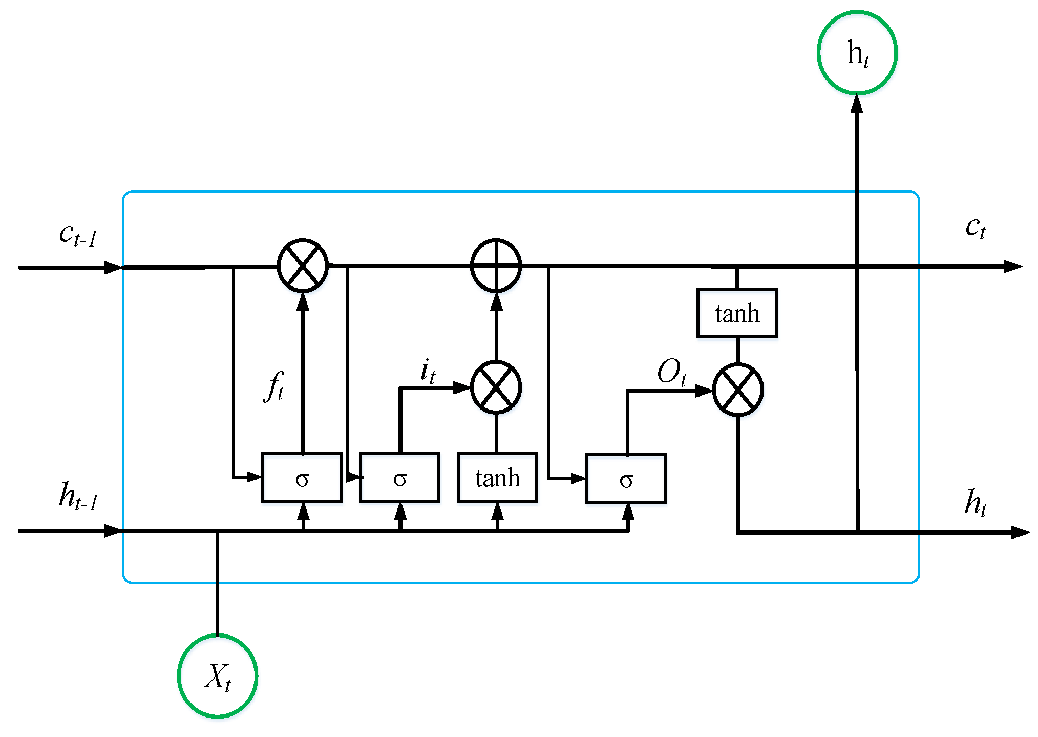
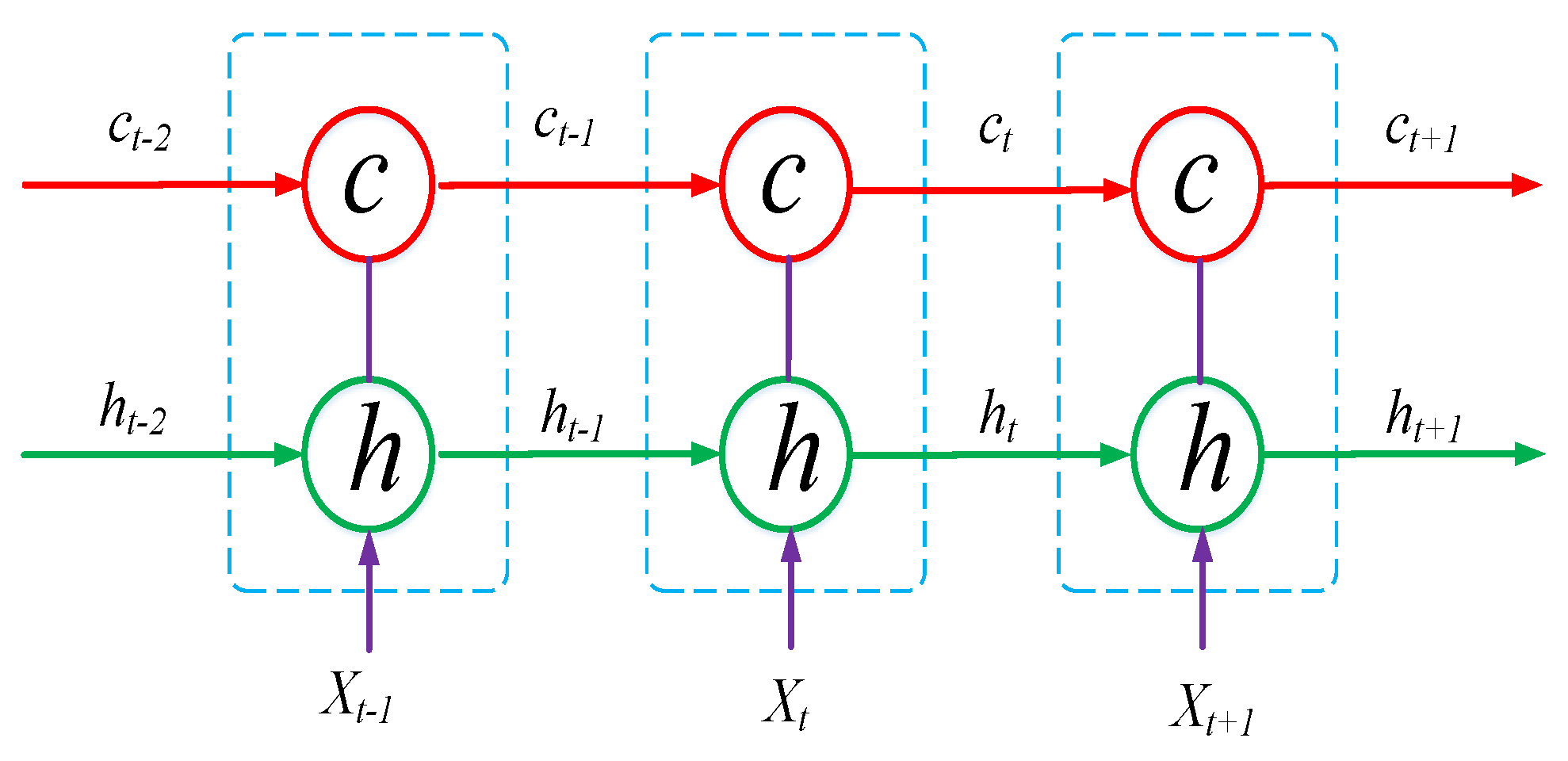
As artificial intelligence technology has developed the adoption of DNN has significantly increased. LSTM is a DNN algorithm, which can be effective for any type of time series data [34]. LSTM is an artificial RNN architecture applied in the field of deep learning. Unlike classical feedforward neural networks, LSTM has feedback connections. Hence, LSTM has good performance in capturing long-term dependencies within a sequence, and is suitable for algorithms in condition monitoring [35], because the sensor data collected from wind turbines is time series data within a sequence. The architecture of the LSTM algorithm is shown in Figure 1 and Figure 2. This algorithm is able to describe nonlinear dynamic systems by mapping input sequences to output sequences. A classical architecture is usually composed of a cell and three gates; the cell is the memory part of the LSTM unit; gates are used to control the flow of information inside the LSTM unit, including an input gate, an output gate and a forget gate.
Actually, the LSTM algorithm is a special instance of an RNN that is more suitable for processing long-term dependency problems. The LSTM algorithm has a cell state that is used to store long-term information in the hidden layer. The current-time input vector is the input data to the LSTM model at time t; is the last time output vector; and represents the last time cell state. In Figure 1, and represent the forget gate and the input gate, which are used to control the cell state of the model. Essentially, forget gates and input gates are designed to restrict the information flow. σ is sigmoid function. The forget gate controls the last cell state information transmitted to the current cell state . This procedure is described in Equation (2),
where is the activate function that achieves the sigmoid nonlinear function, is the forget gate weight matrix, represents the bias vector of the forget gate, and is the combination vector of the last time output vector and the current time input vector .
The input gate controls the current input information transmitted to the current cell state , represented by Equation (3).
where is the weight matrix of the input gate, is the bias vector of the input gate. To obtain the state of the current input, , can be calculated as
where and are the weight matrix and the bias vector respectively, is the hyperbolic tangent function.
The current cell state can then be obtained from Equation (5) which considers both the forget gate and the input gate.
where * describes element-wise multiplication between vectors.
The information flowing from the current cell state is controlled by the output gate to the current output, described by
where is the weight matrix, is the bias vector.
Finally, the output gate and the current cell state determine the output of LSTM model shown in Equation (7)
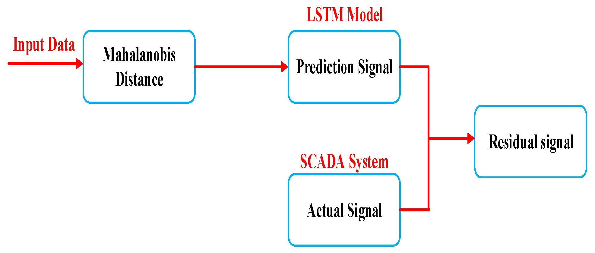
The framework of the proposed condition monitoring method is illustrated in Figure 3. The input data is first processed by the MD method, which reduces the input data quantity to the prediction model, and significantly decreases the required training time and prediction time of the model. Actual data acquired from the turbine SCADA system is then compared to the prediction data obtained from trained LSTM for the corresponding input data. Finally, the residual signal is used to diagnose the occurrence of faults.
4. Case Study
Most modern wind farms are equipped with the SCADA systems that connect each wind turbine and the meteorological station at the site, to a remote central server. In this paper, the SCADA data was collected from a commercial wind farm over a 12-month period and consists of 121 parameters. In order to decrease the number of operational data collected from operating wind turbines, wind turbine SCADA data, sampled at the seconds, is usually recorded at 5 min interval. It means that there is a five-minute interval between two sampling data. The wind turbine studied was 2.5 MW with a doubly-fed induction generator (DFIG) in located site in SE China.
4.1. Parameter Selection for LSTM
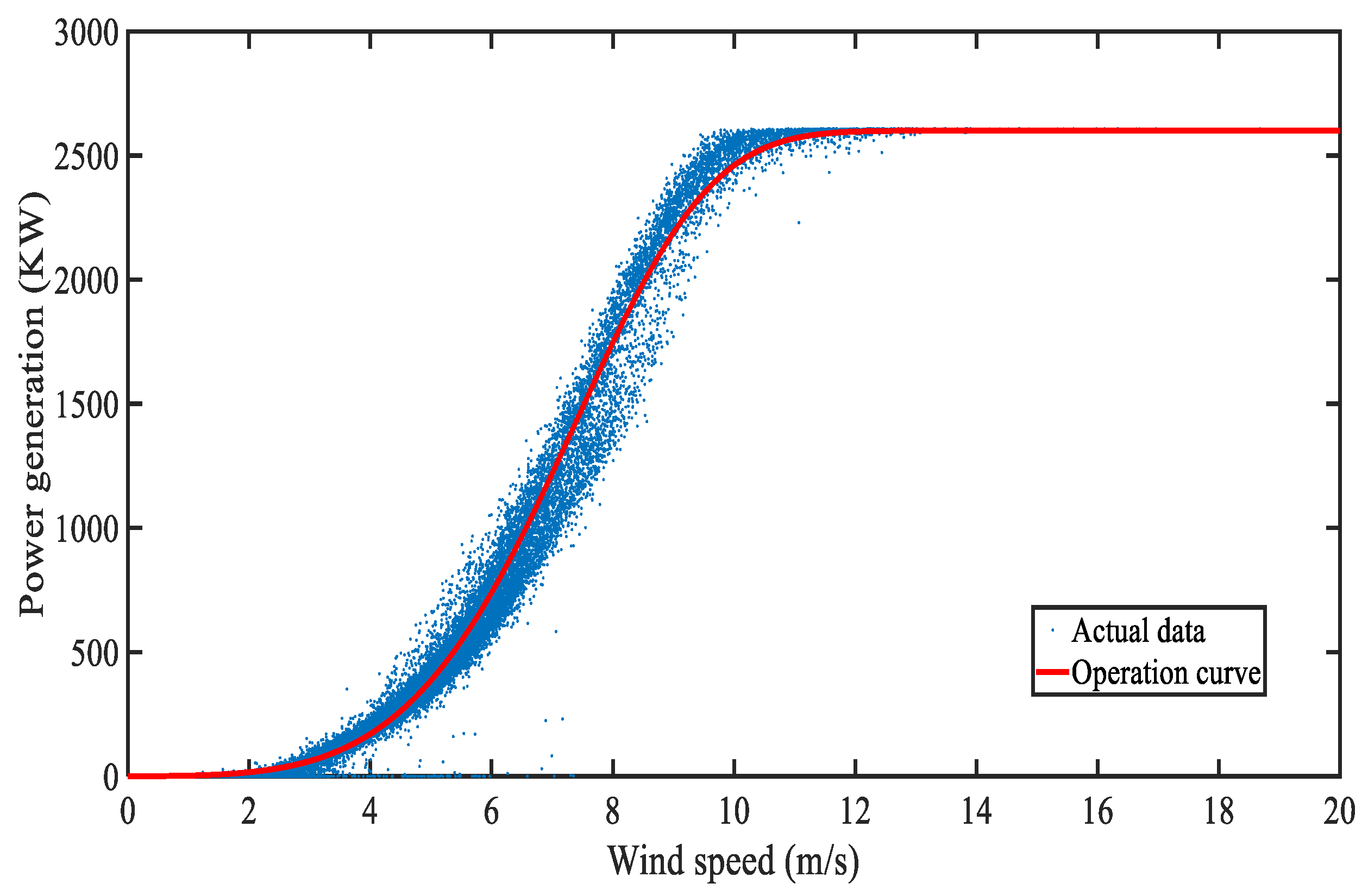
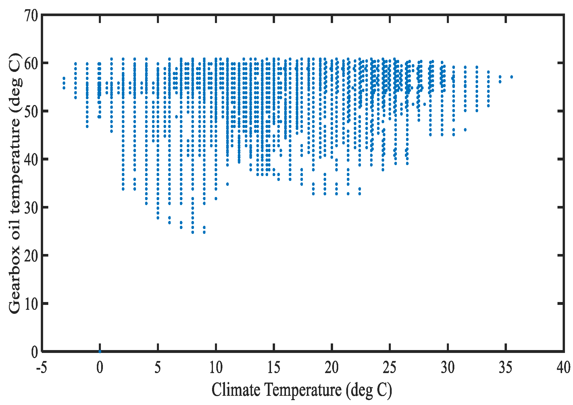
Figure 4 describes a power curve from the wind turbine. It can be seen that power output changes with the cube of the wind speed below the rated wind speed of 10 m/s. When the wind speed is below the cut-in of 3 m/s, the torque from the rotor is insufficient to generate any power. When the wind speed is higher than the cut-out speed of 20 m/s, the turbine is shut down to protect it. When the wind speed is above the rated speed but below the cut-out speed, the power output of the turbine is restricted to the rated power. It is worth noting that the accuracy of the condition monitoring prediction model is not only determined by the parameters of the model, but also by the selection of input variables. For example, one critical factor that affects the heat dissipation of the gearbox is air temperature. The relationship between the gearbox oil temperature of the wind turbine and the air ambient temperature is described in Figure 5. When the air temperature is high heat dissipation by the gearbox is worse than at low temperatures. So, it is clear that the temperature of the gearbox can change over a wide range during winter months and over a smaller range in the summer. In both the power curve and the relationship between the gearbox oil temperature and air temperature, it can be seen that the temperature-based condition monitoring model is non-linear. Hence, LSTM algorithm is very suitable for this application.
In this paper, the MD method is adopted to reduce the number of input variables. However, optimal input variables to be processed should be selected. To demonstrate the impact of parameter selection, a comparative analysis is provided. Four relationships are considered, including wind speed with power output, wind speed with air temperature, power output with air temperature, and a combination of wind speed, power output, and air temperature.
The prediction models are developed to provide the gearbox oil temperature in the wind turbine. The root mean square error (RMSE) value is a widely used parameter to measure how well the models explain the actual data. Details of the prediction model accuracy considering different input variables are provided in Table 1. The RMSE of the prediction models considering the combined 3-input scenario (power generation of the wind turbine, air temperature, and wind speed) is smaller than that of the 2-input scenarios (wind speed with power output, wind speed with air temperature, and power output with air temperature), reaching 0.061 for the 3-input case. The above results indicate that the data-driven prediction model trained with 3-input variables is more accurate than the models trained with 2-input variables. Hence, the data-driven prediction models developed in following case studies are based on 3-input variables.
4.2. CASE 1: Condition Monitoring Based on the Gearbox Oil Temperature
In order to validate the effectiveness of the proposed method for detecting faults in the gearbox, the actual SCADA data collected from a commercial turbine with a gearbox fault has been compared with the corresponding model output predicted by the reference wind turbine models (the reference wind turbines have no faults). The MD value combinations of wind speed, power generation, and air temperature are used as the input to the prediction model. Study case 1 applies the proposed method to predict gearbox oil temperature for gearbox condition monitoring. The actual temperature signal of gearbox oil obtained from the SCADA system is compared to the LSTM model prediction output, and subsequently used to detect the gearbox fault. The data of wind speed, power generation, and air temperature from the healthy wind turbine is first processed by the MD method, and then corresponding MD values are used as the training dataset to obtain the parameters of LSTM prediction model.
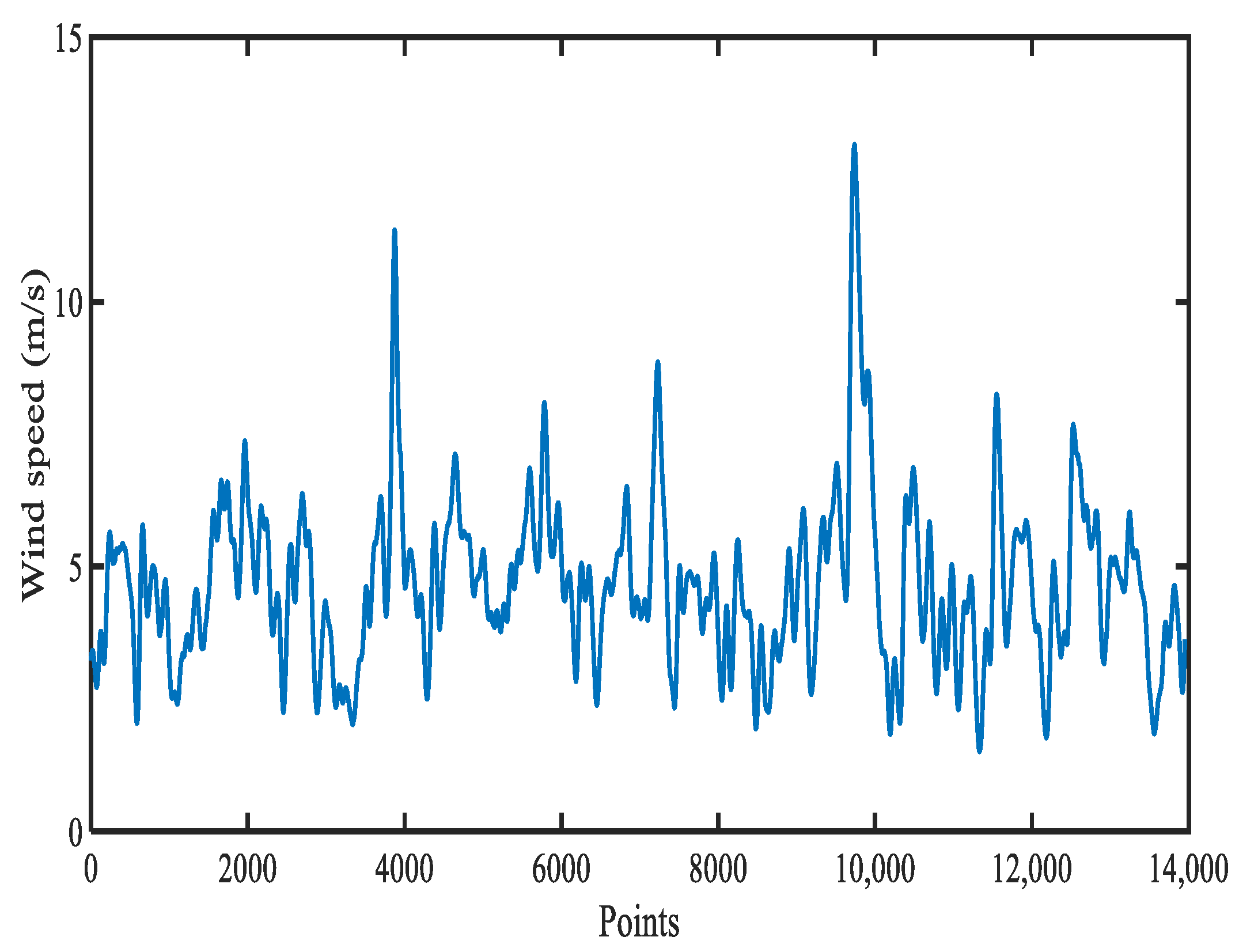
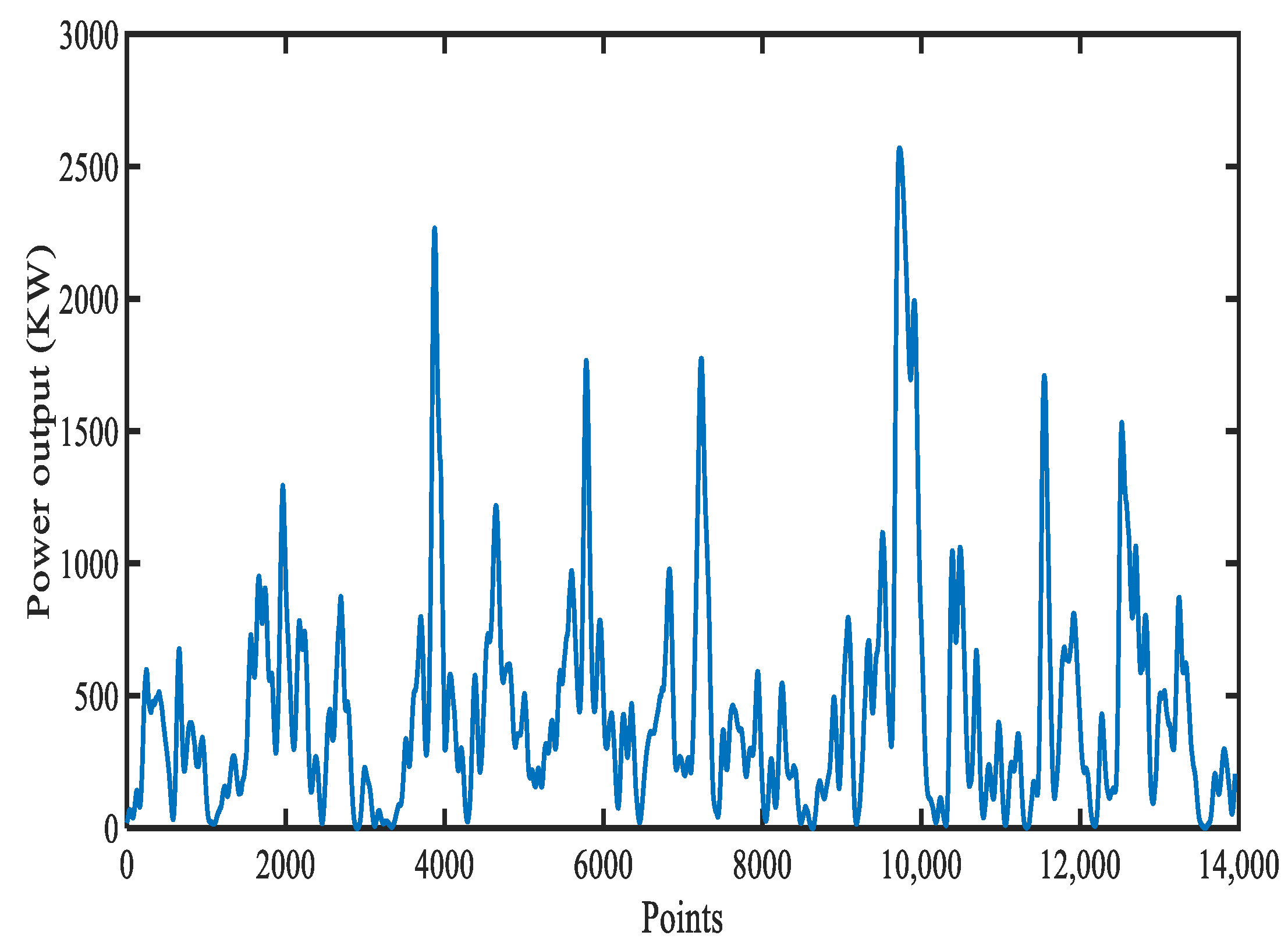
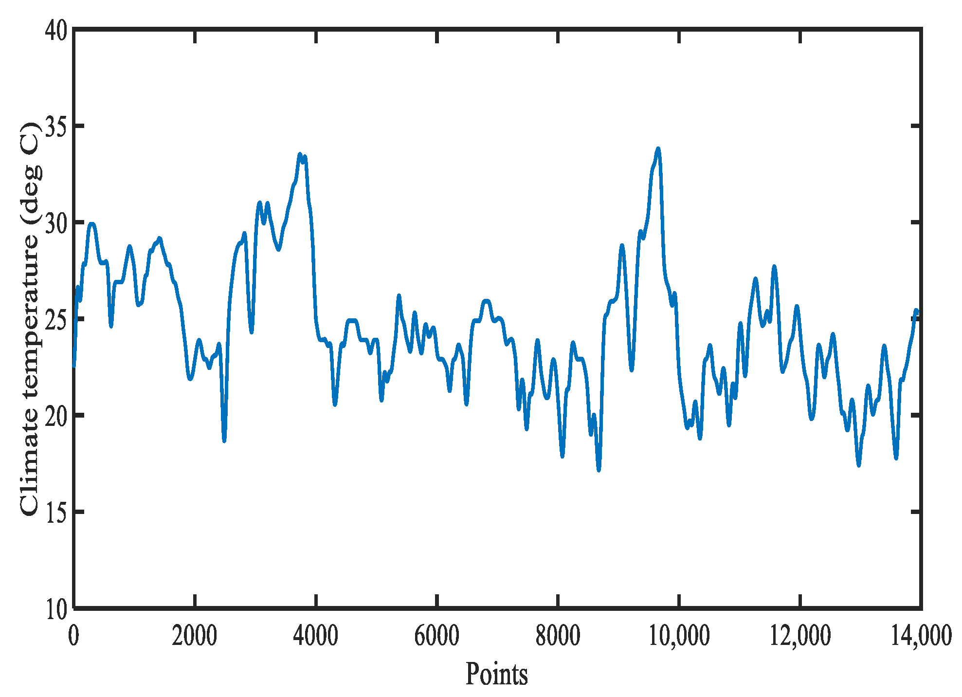
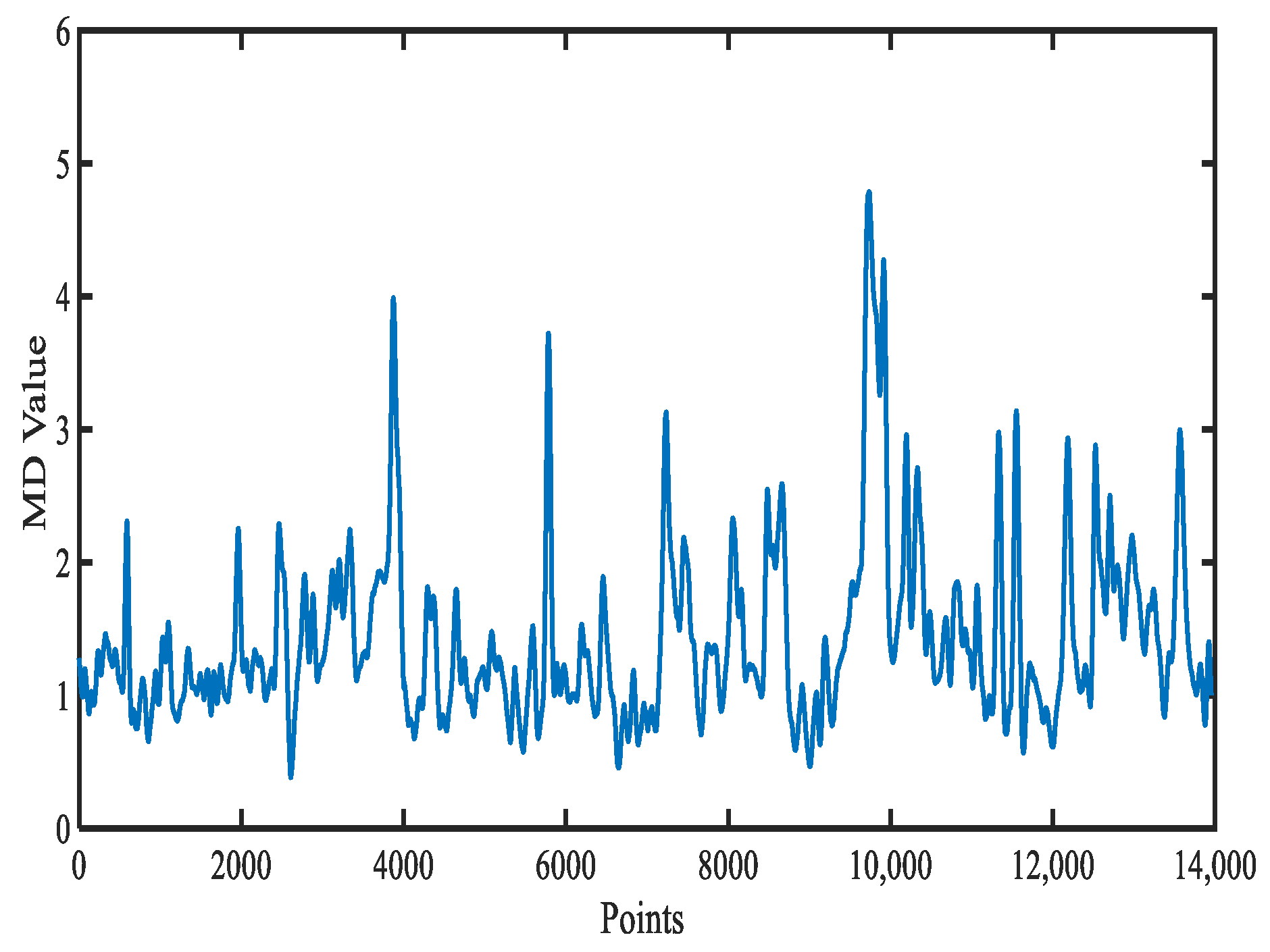
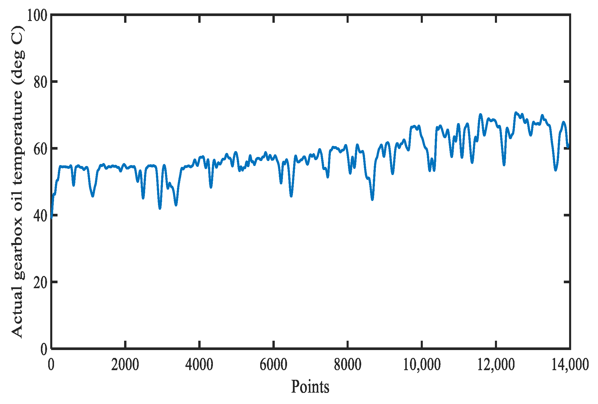
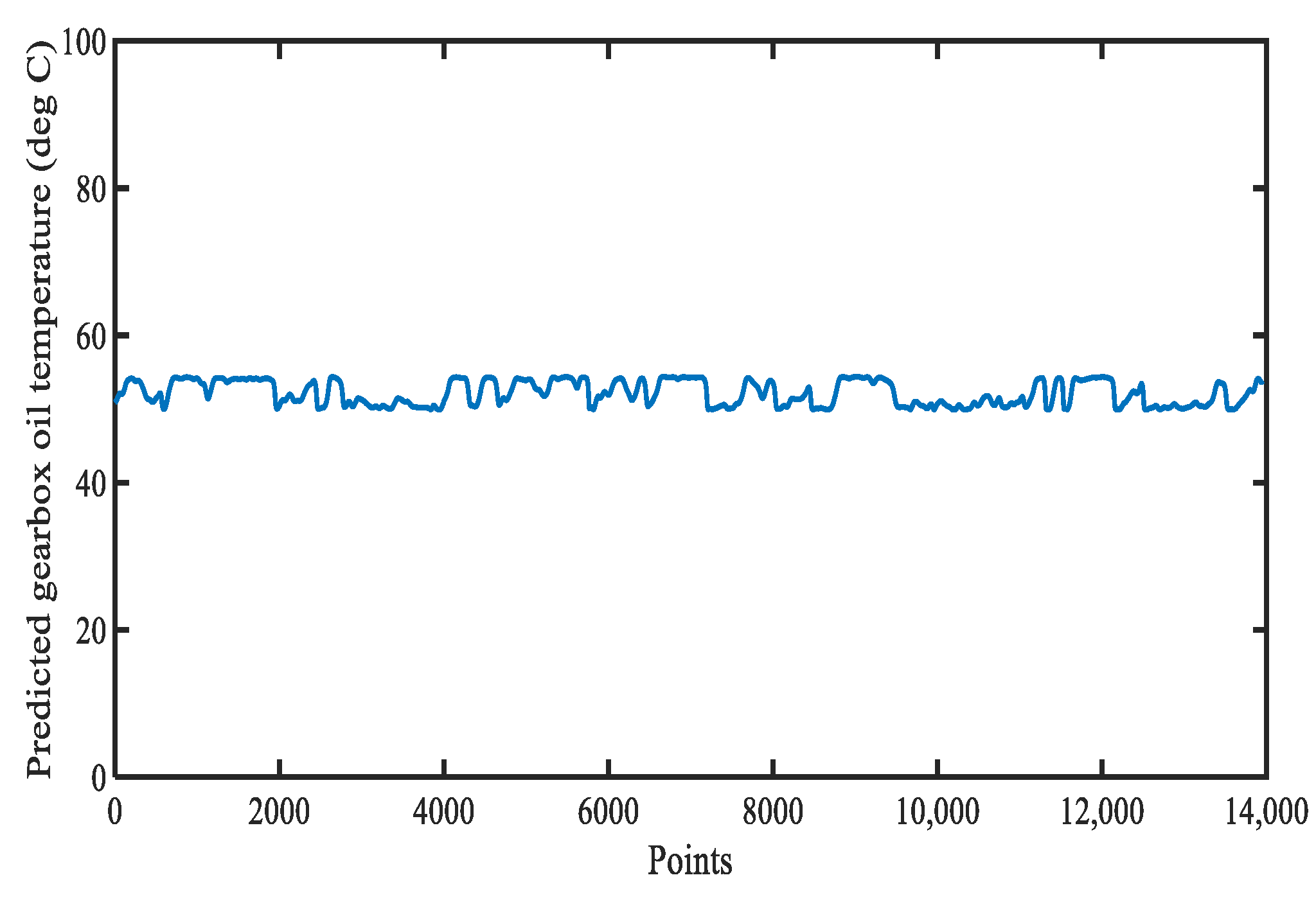
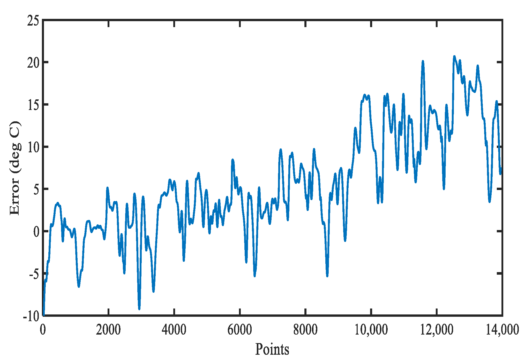
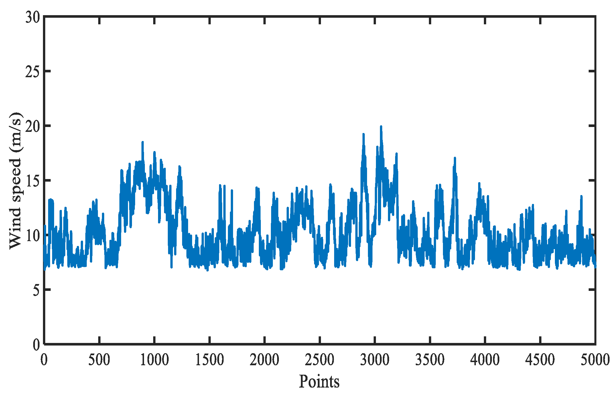
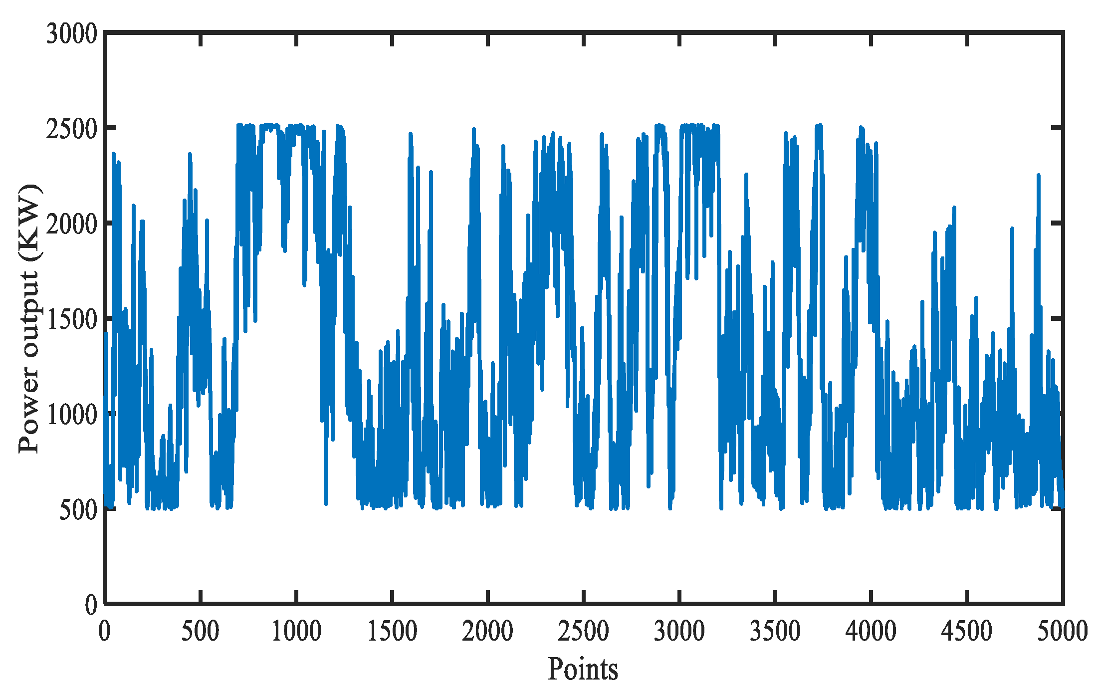
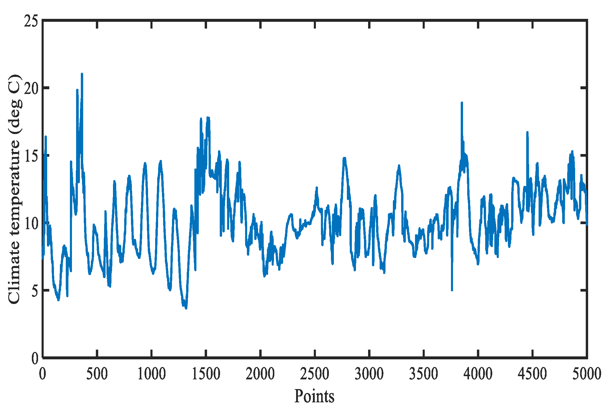
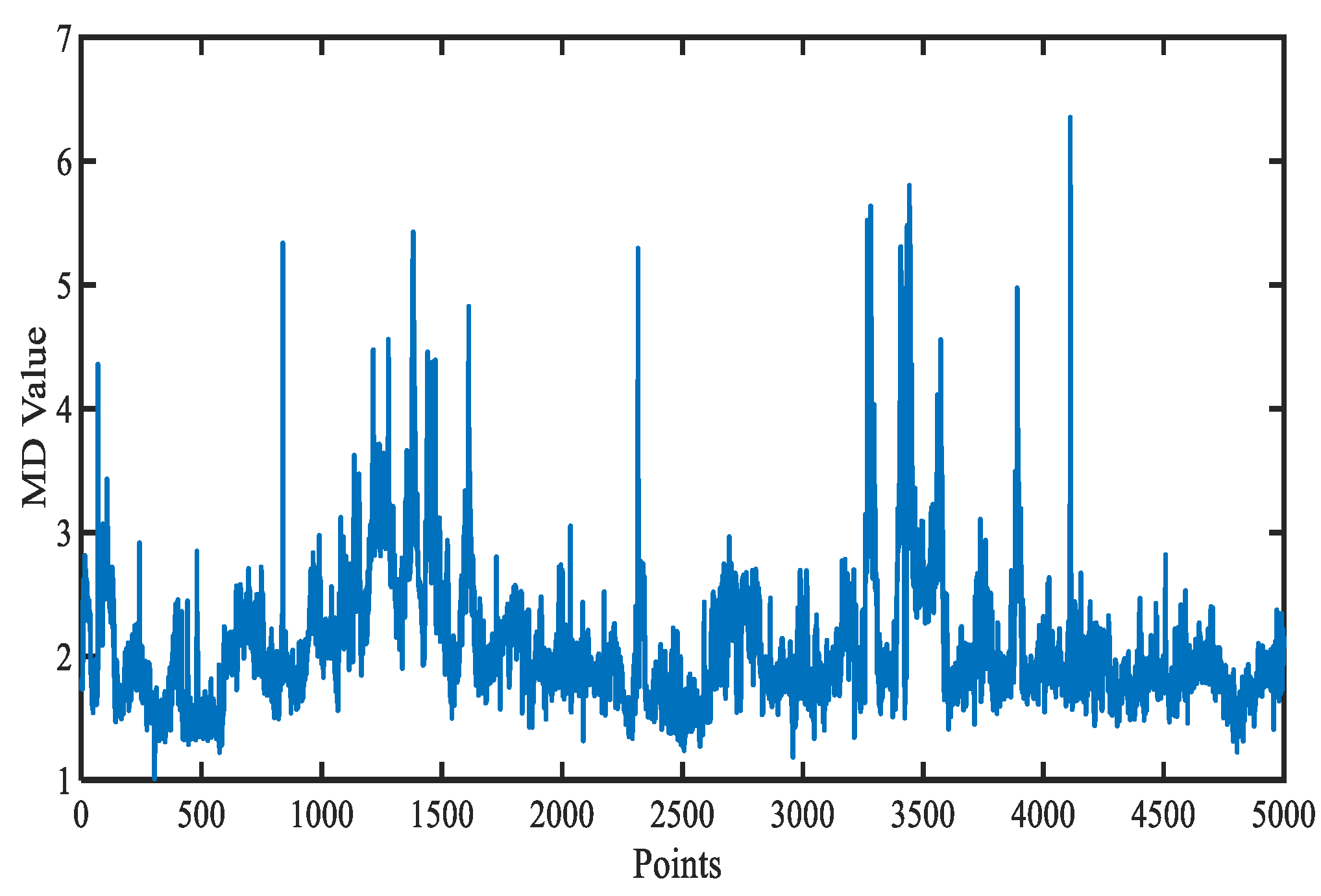
In this case study, Figure 6 shows the wind speed collected from the wind farm. The corresponding wind turbine power output and actual air temperature are given in Figure 7 and Figure 8, respectively. Figure 9 shows the MD value combinations of wind speed, power generation, and air temperature, which are the inputs to the prediction model. Figure 10 illustrates the actual gearbox oil temperature from the SCADA system in the turbine with a gearbox fault. Figure 11 shows the LSTM prediction model output gearbox oil temperature. Figure 12 describes the residual signal of the gearbox oil temperature. The residual signals are calculated from the difference between the prediction model output gearbox oil temperature and the actual temperature of the gearbox oil. It can be observed that the error between the actual gearbox oil temperature from the SCADA system and that from the LSTM prediction model has a small increasing trend and a sudden increase at sampling point 9700, indicating the appearance of an abnormal behaviour in the gearbox. The faults occurring in the gearbox can be investigated in the SCADA data. The alarm logs show that abnormal of gearbox occurred at sampling point 9700, which is consistent with the predicted result based on the LSTM model.
4.3. CASE 2: Condition Monitoring Based on the Generator Bearing Temperature
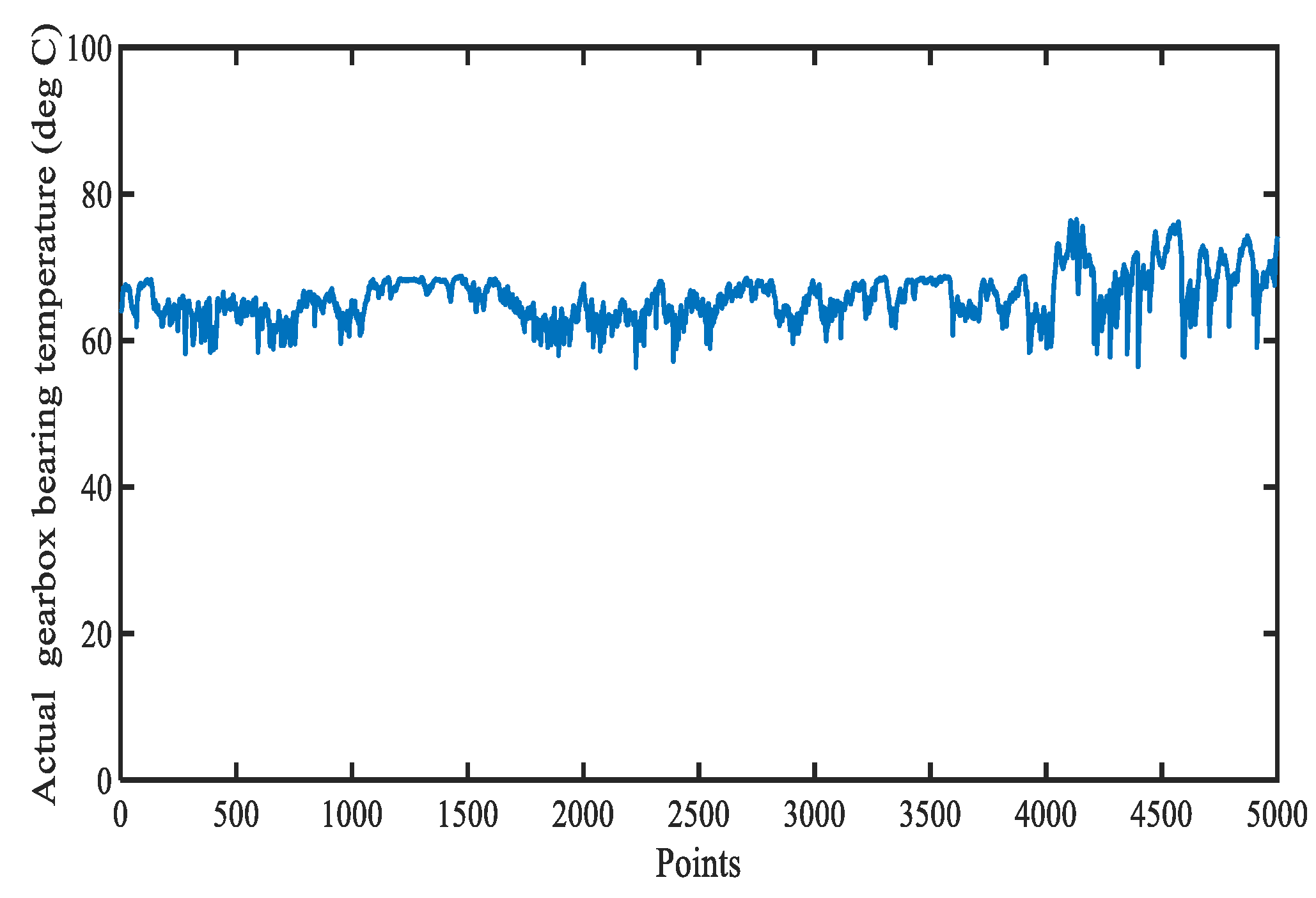
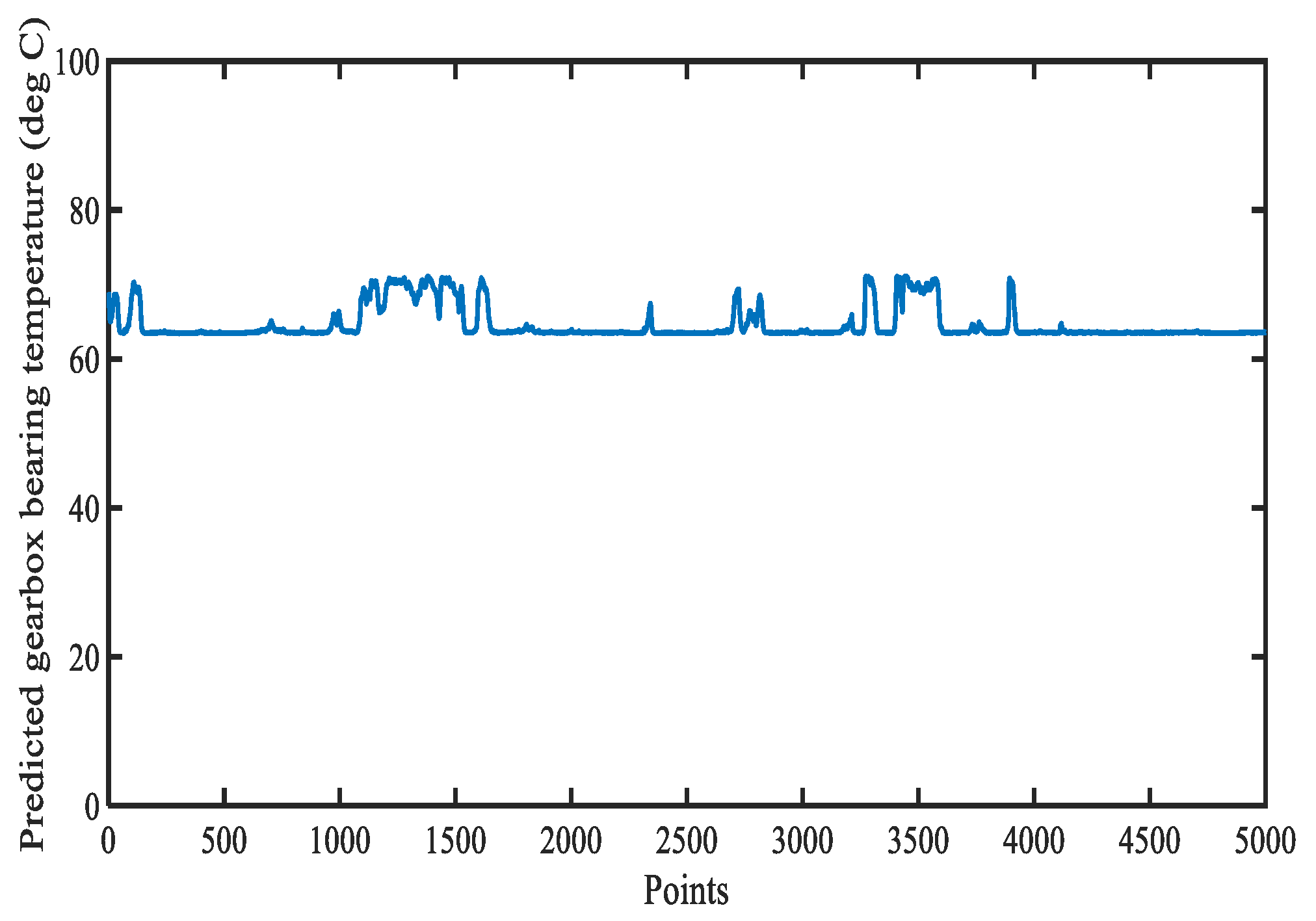
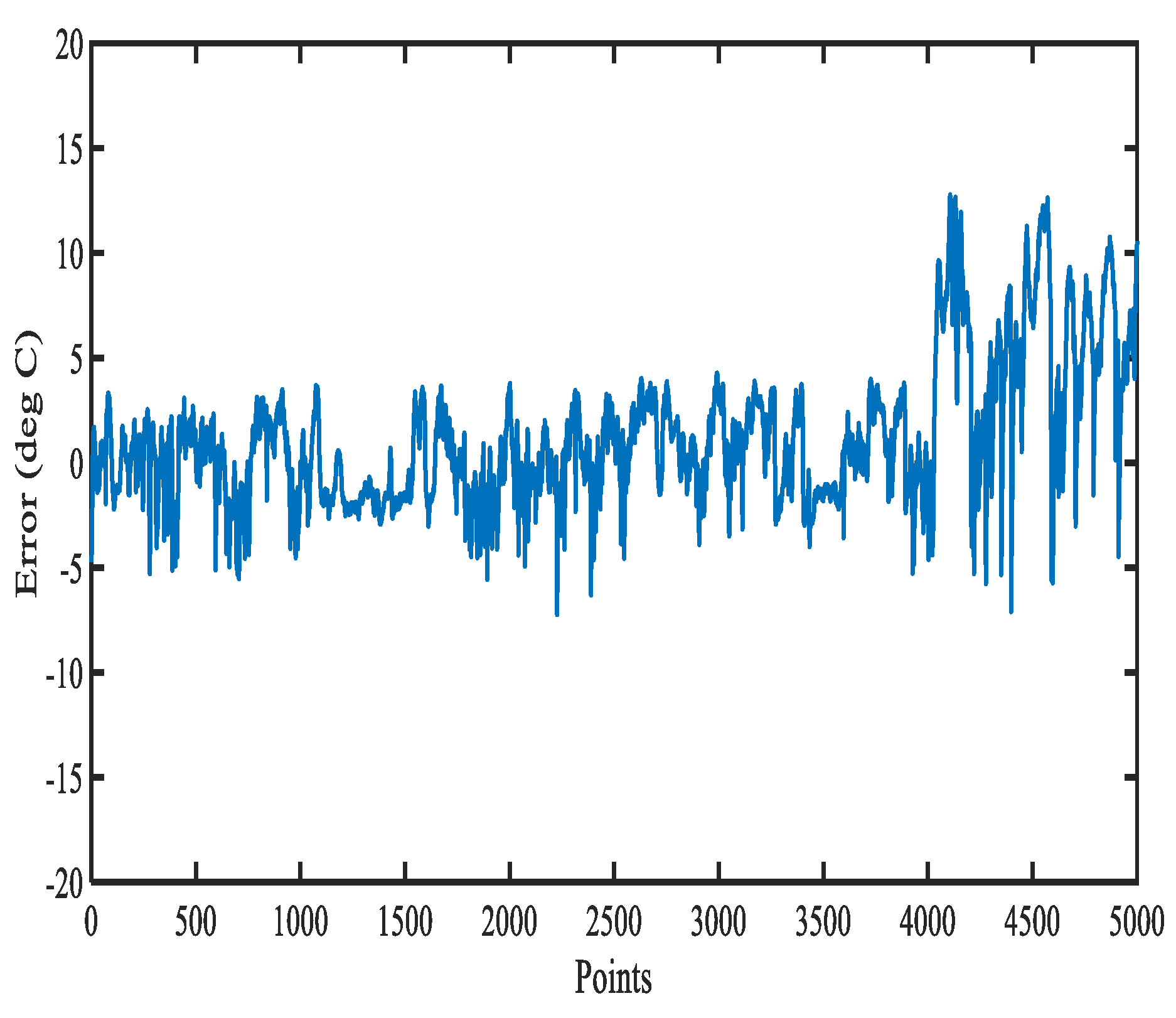
To further validate the proposed method, condition monitoring based on the gearbox bearing temperature is adopted. Figure 13 shows the wind speed measured at the wind farm, and corresponding wind turbine power output and actual air temperature are given in Figure 14 and Figure 15, respectively. In Figure 16, the MD values combination of wind speed, power generation, and air temperature are shown. Figure 17 illustrates the actual gearbox bearing temperature from the SCADA system in the wind turbine with a gearbox bearing fault. Figure 18 shows the LSTM prediction model output gearbox bearing temperature. Figure 19 describes the residual signal of the gearbox bearing temperature. It is obvious that the error between the actual gearbox bearing temperature from the SCADA system and from the LSTM prediction model has a rapid increasing trend at sampling point 4000, which indicates a system abnormal occurred in the gearbox bearing.
The faults occurring in the gearbox bearing can be investigated in the SCADA data and from the alarm logs that record fault information. The alarm logs show that abnormal of a gearbox bearing appeared at sampling point 4000, which is consistent with the predicted result based on the LSTM model.
To validate the prediction performance of LSTM, backpropagation (BP) neural network was applied to both study cases as well. The BP based models can detect a system abnormal occurred in the gearbox bearing or gearbox at the same sampling point as LSTM models, which confirms the detection capability of LSTM models. So RMSE value is used to further compare the performance of LSTM based models to that of BP based models. Table 2 shows the RMSE values from both BP and LSTM models. It shows that the RMSE values from LSTM models are approximately 4% lower than that from BP models for both cases, which means that LSTM models have better performance for condition monitoring than BP based models.
5. Conclusions
In this paper, a novel condition monitoring model of the wind turbine based on Long Short-Term Memory has been presented. SCADA data collected from a commercial wind farm has been adopted to validate the performance of the proposed model. Two case studies have been carried out to illustrate the wind turbine condition monitoring by using gearbox oil temperature and gearbox bearing temperature. The data analysis results show that LSTM has better prediction performance than conventional back propagation neural network algorithms. The RMSE values for the LSTM models are reduced by about 4% compared to traditional back propagation neural network model in both case studies. Moreover, the number of input data values has been reduced to one third, by adopting the MD method. Hence, the proposed method is suitable to be applied in the condition monitoring system, which can reduce the cost of condition monitoring and increase monitoring accuracy.
Author Contributions
P.Q. and X.T. carried out most of the work presented here; J.K. and T.-H.G. revised the contents and reviewed the manuscript; and J.L.Y.L. contributed to the writing and summarizing proposed ideas of Section 3.
Funding
This research was funded by innovate UK grant number [86300-542369].
Conflicts of Interest
The authors declare no conflict of interest.
References
- Jiang, L.; Chi, Y.; Qin, H.; Pei, Z.; Li, Q.; Liu, M. Wind Energy in China. IEEE Power Energy Mag. 2011, 9, 36–46. [Google Scholar] [CrossRef]
- Qian, P.; Ma, X.; Zhang, D.; Wang, J. Data-Driven Condition Monitoring Approaches to Improving Power Output of Wind Turbines. IEEE Trans. Ind. Electron. 2019, 66, 6012–6020. [Google Scholar] [CrossRef]
- Pattison, D.; Garcia, M.S.; Xie, W.; Quail, F.; Revie, M.; Whitfield, R.I.; Irvine, I. Intelligent integrated maintenance for wind power generation. Wind Energy 2016, 19, 547–562. [Google Scholar] [CrossRef]
- Qian, P.; Ma, X.; Cross, P. Integrated data-driven model-based approach to condition monitoring of the wind turbine gearbox. IET Renew. Power Gener. 2017, 11, 1177–1185. [Google Scholar] [CrossRef]
- Qiu, Y.; Zhang, W.; Infield, D.; Feng, Y.; Sun, J. Applying thermophysics for wind turbine drivetrain fault diagnosis using SCADA data. IET Renew. Power Gener. 2016, 10, 661–668. [Google Scholar] [CrossRef] [Green Version]
- Zhang, D.; Qian, L.; Mao, B.; Huang, C.; Huang, B.; Si, Y. A Data-Driven Design for Fault Detection of Wind Turbines Using Random Forests and XGboost. IEEE Access 2018, 6, 21020–21031. [Google Scholar] [CrossRef]
- Vieira, R.J.D.A.; Sanz-Bobi, M.A. Failure Risk Indicators for a Maintenance Model Based on Observable Life of Industrial Components with an Application to Wind Turbines. IEEE Trans. Reliab. 2013, 62, 569–582. [Google Scholar] [CrossRef]
- Guo, P.; Fu, J.; Yang, X. Condition Monitoring and Fault Diagnosis of Wind Turbines Gearbox Bearing Temperature Based on Kolmogorov-Smirnov Test and Convolutional Neural Network Model. Energies 2018, 11, 2248. [Google Scholar] [CrossRef]
- Qiao, W.; Lu, D. A Survey on Wind Turbine Condition Monitoring and Fault Diagnosis—Part II: Signals and Signal Processing Methods. IEEE Trans. Ind. Electron. 2015, 62, 6546–6557. [Google Scholar] [CrossRef]
- Tian, X.; Gu, J.X.; Rehab, I.; Abdalla, G.M.; Gu, F.; Ball, A. A robust detector for rolling element bearing condition monitoring based on the modulation signal bispectrum and its performance evaluation against the Kurtogram. Mech. Syst. Signal Process. 2018, 100, 167–187. [Google Scholar] [CrossRef]
- Gong, X.; Qiao, W. Current-Based Mechanical Fault Detection for Direct-Drive Wind Turbines via Synchronous Sampling and Impulse Detection. IEEE Trans. Ind. Electron. 2015, 62, 1693–1702. [Google Scholar] [CrossRef]
- Qian, P.; Ma, X.; Zhang, D. Estimating Health Condition of the Wind Turbine Drivetrain System. Energies 2017, 10, 1583. [Google Scholar] [CrossRef]
- Tautz-Weinert, J.; Watson, S.J. Using SCADA data for wind turbine condition monitoring—A review. IET Renew. Power Gener. 2017, 11, 382–394. [Google Scholar] [CrossRef]
- Chen, Q.; Xu, G.; Liu, G.; Zhao, W.; Lin, Z.; Liu, L. Torque ripple reduction in five-phase interior permanent magnet motors by lowering interactional MMF. IEEE Trans. Ind. Electron. 2018, 65, 8520–8531. [Google Scholar] [CrossRef]
- Guo, P.; Bai, N. Wind Turbine Gearbox Condition Monitoring with AAKR and Moving Window Statistic Methods. Energies 2011, 4, 2077–2093. [Google Scholar] [CrossRef] [Green Version]
- Mahmoud, T.; Dong, Z.Y.; Ma, J. An advanced approach for optimal wind power generation prediction intervals by using self-adaptive evolutionary extreme learning machine. Renew. Energy 2018, 126, 254–269. [Google Scholar] [CrossRef]
- Jiang, Y.-G.; Wu, Z.; Tang, J.; Li, Z.; Xue, X.; Chang, S.-F. Modeling Multimodal Clues in a Hybrid Deep Learning Framework for Video Classification. IEEE Trans. Multimedia 2018, 20, 3137–3147. [Google Scholar] [CrossRef] [Green Version]
- Yang, S.; Li, W.; Wang, C. The intelligent fault diagnosis of wind turbine gearbox based on artificial neural network. In Proceedings of the 2008 International Conference on Condition Monitoring and Diagnosis, Beijing, China, 21–24 April 2008. [Google Scholar]
- Li, Y.; Wu, H.; Liu, H. Multi-step wind speed forecasting using EWT decomposition, LSTM principal computing, RELM subordinate computing and IEWT reconstruction. Energy Convers. Manag. 2018, 167, 203–219. [Google Scholar] [CrossRef]
- Elobaid, L.M.; Abdelsalam, A.K.; Zakzouk, E.E. Artificial neural network-based photovoltaic maximum power point tracking techniques: A survey. IET Renew. Power Gener. 2015, 9, 1043–1063. [Google Scholar] [CrossRef]
- Zhao, H.; Liu, H.; Hu, W.; Yan, X.; Hongshan, Z.; Huihai, L.; Wenjing, H.; Xihui, Y. Anomaly detection and fault analysis of wind turbine components based on deep learning network. Renew. Energy 2018, 127, 825–834. [Google Scholar] [CrossRef]
- Tang, J.; Deng, C.; Huang, G.-B.; Zhao, B. Compressed-Domain Ship Detection on Spaceborne Optical Image Using Deep Neural Network and Extreme Learning Machine. IEEE Trans. Geosci. Remote Sens. 2015, 53, 1174–1185. [Google Scholar] [CrossRef]
- Bedi, J.; Toshniwal, D. Empirical Mode Decomposition Based Deep Learning for Electricity Demand Forecasting. IEEE Access 2018, 6, 49144–49156. [Google Scholar] [CrossRef]
- Tang, J.; Deng, C.; Huang, G.B. Extreme Learning Machine for Multilayer Perceptron. IEEE Trans. Neural Netw. Learn. Syst. 2016, 27, 809–821. [Google Scholar] [CrossRef] [PubMed]
- Xu, C.; Shen, J.; Du, X.; Zhang, F. An Intrusion Detection System Using a Deep Neural Network with Gated Recurrent Units. IEEE Access 2018, 6, 48697–48707. [Google Scholar] [CrossRef]
- Zhang, Q.; Li, F.; Long, F.; Ling, Q. Vehicle Emission Forecasting Based on Wavelet Transform and Long Short-Term Memory Network. IEEE Access 2018, 6, 56984–56994. [Google Scholar] [CrossRef]
- Hu, Y.-L.; Chen, L. A nonlinear hybrid wind speed forecasting model using LSTM network, hysteretic ELM and Differential Evolution algorithm. Energy Convers. Manag. 2018, 173, 123–142. [Google Scholar] [CrossRef]
- Lei, J.; Liu, C.; Jiang, D. Fault diagnosis of wind turbine based on Long Short-term memory networks. Renew. Energy 2019, 133, 422–432. [Google Scholar] [CrossRef]
- Shi, X.; Lei, X.; Huang, Q.; Huang, S.; Ren, K.; Hu, Y. Hourly Day-Ahead Wind Power Prediction Using the Hybrid Model of Variational Model Decomposition and Long Short-Term Memory. Energies 2018, 11, 3227. [Google Scholar] [CrossRef]
- Wang, Y.; Xie, D.; Wang, X.; Zhang, Y. Prediction of Wind Turbine-Grid Interaction Based on a Principal Component Analysis-Long Short Term Memory Model. Energies 2018, 11, 3221. [Google Scholar] [CrossRef]
- Yang, R.; Huang, M.; Lu, Q.; Zhong, M. Rotating Machinery Fault Diagnosis Using Long-short-term Memory Recurrent Neural Network. IFAC-PapersOnLine 2018, 51, 228–232. [Google Scholar] [CrossRef]
- Gao, Y.; Wang, M.; Ji, R.; Wu, X.; Dai, Q. 3-D Object Retrieval With Hausdorff Distance Learning. IEEE Trans. Ind. Electron. 2014, 61, 2088–2098. [Google Scholar] [CrossRef]
- Zeng, M.; Zhang, L.; Tian, C.; Zhao, X.; Wu, Z. Person re-identification based on a novel mahalanobis distance feature dominated KISS metric learning. Electron. Lett. 2016, 52, 1223–1225. [Google Scholar] [CrossRef]
- Duan, Z.; Yang, Y.; Zhang, K.; Ni, Y.; Bajgain, S. Improved Deep Hybrid Networks for Urban Traffic Flow Prediction Using Trajectory Data. IEEE Access 2018, 6, 31820–31827. [Google Scholar] [CrossRef]
- López, E.; Valle, C.; Allende, H.; Gil, E.; Madsen, H. Wind Power Forecasting Based on Echo State Networks and Long Short-Term Memory. Energies 2018, 11, 526. [Google Scholar] [CrossRef]
Figure 1.
Diagram of a single layer Long Short-Term Memory cell.

Figure 2.
The temporal-logic framework of a single layer LSTM.

Figure 3.
The framework of the proposed condition monitoring method.

Figure 4.
Power curve of the wind turbine.

Figure 5.
Relationship between the gearbox oil temperature and air temperature.

Figure 6.
Actual wind speed of the wind turbine.

Figure 7.
Actual power generation of the wind turbine.

Figure 8.
Actual air temperature in the wind farm.

Figure 9.
MD value for prediction model input.

Figure 10.
Actual temperature of the gearbox oil obtained from the supervisory control and data acquisition data.
Figure 10.
Actual temperature of the gearbox oil obtained from the supervisory control and data acquisition data.

Figure 11.
Predicted temperature of the gearbox oil gained from the LSTM model.

Figure 12.
Residual temperature of the gearbox oil.

Figure 13.
Actual wind speed of the wind turbine.

Figure 14.
Actual power generation of the wind turbine.

Figure 15.
Actual air temperature in the wind farm.

Figure 16.
Mahalanobis distance value for prediction model input.

Figure 17.
Actual temperature of the gearbox bearing gained from the SCADA model.

Figure 18.
Predicted temperature of the gearbox bearing gained from the LSTM model.

Figure 19.
Residual temperature of the gearbox bearing.


Table 1.
The accuracy of the prediction models considering different input parameters. RMES: root mean square error.
Table 1.
The accuracy of the prediction models considering different input parameters. RMES: root mean square error.
| Input Variables | RMSE Value |
|---|---|
| wind speed, power output | 0.084 |
| wind speed, air temperature | 0.067 |
| power output, air temperature | 0.081 |
| wind speed, power output and air temperature | 0.061 |
Table 2.
Performance comparison of BP and LSTM.
| Case No. | RMSE | |
|---|---|---|
| BP | LSTM | |
| 1 | 0.7983 | 0.7529 |
| 2 | 0.5807 | 0.5400 |
© 2019 by the authors. Licensee MDPI, Basel, Switzerland. This article is an open access article distributed under the terms and conditions of the Creative Commons Attribution (CC BY) license (http://creativecommons.org/licenses/by/4.0/).
Share and Cite
MDPI and ACS Style
Qian, P.; Tian, X.; Kanfoud, J.; Lee, J.L.Y.; Gan, T.-H. A Novel Condition Monitoring Method of Wind Turbines Based on Long Short-Term Memory Neural Network. Energies 2019, 12, 3411. https://doi.org/10.3390/en12183411
AMA Style
Qian P, Tian X, Kanfoud J, Lee JLY, Gan T-H. A Novel Condition Monitoring Method of Wind Turbines Based on Long Short-Term Memory Neural Network. Energies. 2019; 12(18):3411. https://doi.org/10.3390/en12183411
Chicago/Turabian StyleQian, Peng, Xiange Tian, Jamil Kanfoud, Joash Lap Yan Lee, and Tat-Hean Gan. 2019. "A Novel Condition Monitoring Method of Wind Turbines Based on Long Short-Term Memory Neural Network" Energies 12, no. 18: 3411. https://doi.org/10.3390/en12183411
Note that from the first issue of 2016, this journal uses article numbers instead of page numbers. See further details here.