Simplified Method for Analyzing the Availability of Rooftop Photovoltaic Potential
by

Primož Mavsar
1, 
Klemen Sredenšek
2,
Bojan Štumberger
2,3,
Miralem Hadžiselimović
2,3 and
Sebastijan Seme
2,3,* 1
Regional Surveying and Mapping Authority Novo mesto, Ljubljanska cesta 26, 8000 Novo mesto, Slovenia
2
Faculty of Energy Technology, University of Maribor, Hočevarjev trg 1, 8270 Krško, Slovenia
3
Faculty of Electrical Engineering and Computer Science, University of Maribor, Koroška cesta 46, 2000 Maribor, Slovenia
*
Author to whom correspondence should be addressed.
Energies 2019, 12(22), 4233; https://doi.org/10.3390/en12224233
Submission received: 6 October 2019
/
Revised: 28 October 2019
/
Accepted: 2 November 2019
/
Published: 6 November 2019
(This article belongs to the Special Issue PV Systems: from Small- to Large-Scale)
Abstract
:This paper presents a new simplified method for analyzing the availability of photovoltaic potential on roofs. Photovoltaic systems on roofs are widespread as they represent a sustainable and safe investment and, therefore, a means of energy self-sufficiency. With the growth of photovoltaic systems, it is also crucial to correctly evaluate their global efficiency. Thus, this paper presents a comparison between known methods for estimating the photovoltaic potential (as physical, geographic and technical contributions) on a roof and proposes a new simplified method, that takes into account the economic potential of a building that already has installed a photovoltaic system. The measured values of generated electricity of the photovoltaic system were compared with calculated photovoltaic potential. In general, the annual physical, geographic, technical and economic potentials were 1273.7, 1253.8, 14.2 MWh, and 279.1 Wh, respectively. The analysis of all four potentials is essential for further understanding of the sustainable and safe investment in photovoltaic systems.
1. Introduction
Population growth and, consequently, per capita consumption are increasing worldwide in developed countries. The solution to this problem is to integrate renewable energy in urban areas [1,2,3,4,5]. Renewable energy integration is suitable for all economies in urban areas, whether developed, emerging or underdeveloped [6]. To successfully continue the integration of the photovoltaic (PV) systems into the grid and to improve current policies and directives, it is essential to correctly estimate rooftop PV potential [7,8,9,10,11,12,13,14,15,16]. In [17], the advantages and disadvantages of various methods for estimating rooftop suitability for PV installations are described. The analysis was carried out with the constant-value method, manual selection method and Geographic Information System (GIS)-based method [18], which are (according to [17]) the three most important methods for estimating rooftop suitability for PV installations. The rooftop PV potential can be hierarchically divided into four steps: physical, geographic, technical [19,20], and economic potential [21,22,23]. All four steps are graphically presented in Figure 1.
A similar estimation of PV potential was performed by Hong et al. [24]. The first steps were performed using Hillshade analysis, while in [25], a new economic potential was added, taking into account spatial and temporal diversity. In places where buildings are of higher dimensions, the installation of PV systems may not always be suitable due to the shading of surrounding objects. Therefore, in order to correctly evaluate the geographic potential, it is imperative to take into account the shading caused by the surrounding objects. Accordingly, several studies analyzed the geographic potential of building rooftops using various methods to determine the shadow effect [26,27,28,29,30]. Lukač et al. [31,32], using graphics processing units (GPU), and light detection and ranging (LiDAR) data, showed how the determination of shadows can drastically reduce the estimated PV potential. Rodriguez et al. [4] presented a new methodology approach for determining the PV potential at an urban and regional scale using a description of CityGML geometry. The proposed method determines the PV potential for each building separately using building-by-building analysis, irradiance simulation, and reduction factors for energy yield. Furthermore, PV potential greatly depends on terrain configuration and on the inclination and orientation of the PV systems. Seme et al. [33] compared energy production between differently inclined and oriented PV systems under outdoor conditions. The basis for determining the geographic potential in this paper is the use of LiDAR data that show a 3D representation of the terrain surface, with high accuracy for large geometrically simple roofs [34].
The European Union (EU) directive on renewable energy sources (2009/28/ES) in self-sufficient energy communities at the local and national levels gives producers and consumers a new way of trading electricity in the retail market. Thus, the producer can sell electricity to consumers without intermediaries. In the near future, each producer will have the opportunity to sell electricity directly to the electricity market. Therefore, it makes sense to introduce the economic potential that describes the economic aspect of eligibility of the PV system. The economic potential takes into account the technical generation of electricity, the hourly price of electricity on the market, the investment cost, and the installed power of the PV system. Maciejowska et al. [35], presents forecasts of the price spread between the intraday/balancing and day-ahead markets in the decision process. Therefore, economic potential shows that the economic and technical potential are not proportional, but it all depends on the price of electricity at a given moment. It is shown that the price of electricity has significantly higher meanings than the projected technical potential. The contribution of this research is the development of a combined procedure for determining photovoltaic potential on rooftops that are suitable for PV installation. Figure 2 shows the location of the Krško-Sevnica School Center, on which the estimation of the rooftop PV potential was performed.
2. Methods
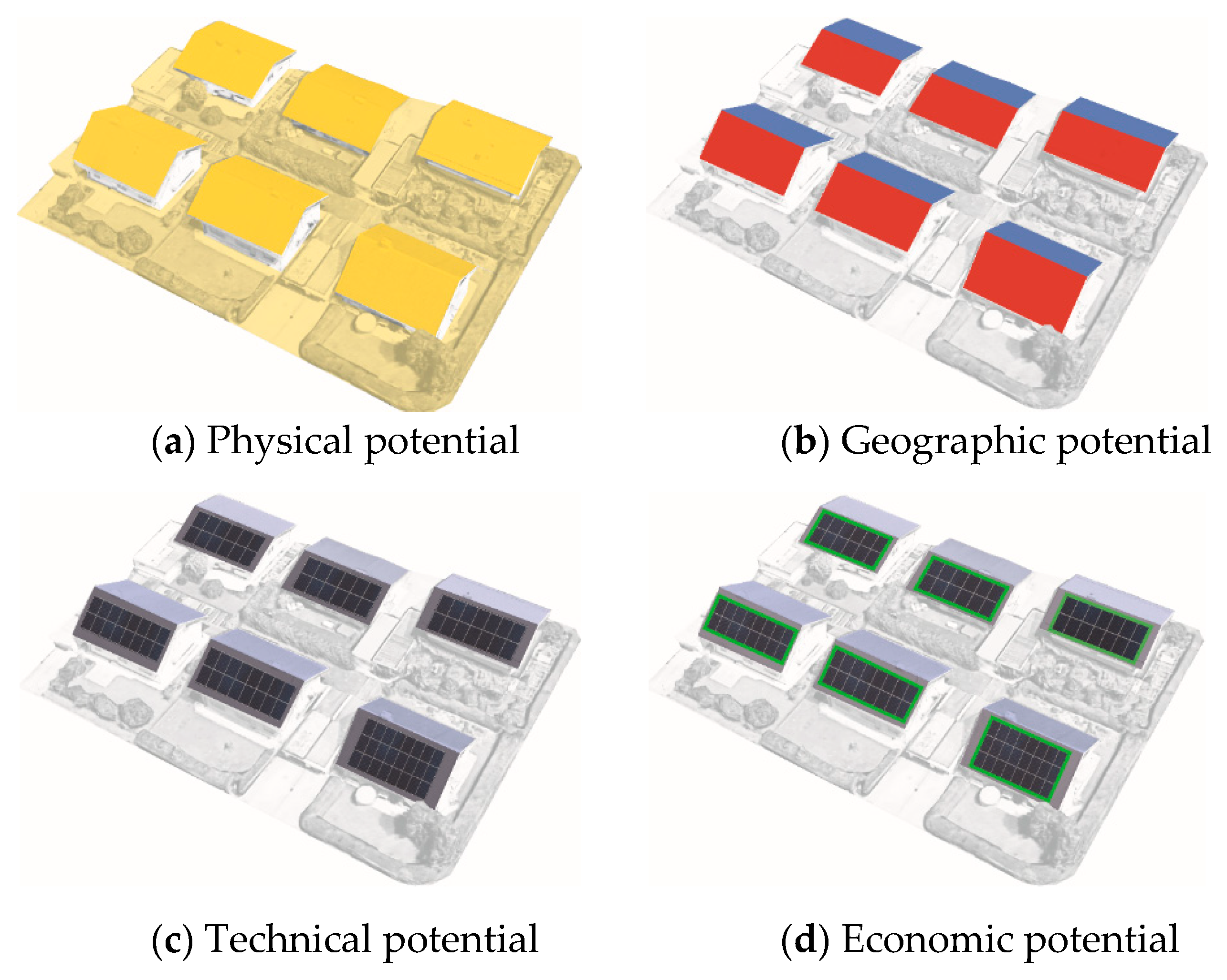
The methodology for estimating the rooftop PV potential is divided into four parts (see Figure 3): (a) calculation of the physical potential; (b) calculation of the geographic potential; (c) calculation of the technical potential; and (d) calculation of the economic potential.
2.1. Physical Potential
The physical potential PP (Wh) is basically the amount of energy that the total area receives over a certain period of time, and can be calculated by Equation (1):
where AT (m2) stands for total rooftop area of the selected location and Gh(t) (W/m2) stands for the global solar radiation on a horizontal surface and can be calculated by Equation (2):
where Gb(t) (W/m2) stands for the beam solar radiation and Gd(t) (W/m2) stands for the diffuse solar radiation on a horizontal surface. Solar radiation data for global and diffuse components are provided in a half-hourly intervals basis by the Slovenian Environment Agency [36].
2.2. Geographic Potential
The geographic potential GP (Wh), is basically the amount of energy that the available area receives over a certain period of time, and can be calculated by Equation (3):
where Aeff stands for effective rooftop area of the selected location, and Gt(t) (W/m2) stands for the total solar radiation on an inclined surface and can be calculated by Equation (4) [37]:
where i (°) stands for the incidence angle of the sun, α (°) stands for solar altitude angle, β (°) stands for inclination angle of the surface above the horizontal, and ρ stands for a surface albedo. To calculate the above-presented parameters, the following parameters must also be considered: declination angle δ (°), solar hour angle ω (°), zenith angle z (°), and solar azimuth angle γ.
Accurate prediction of the geographic potential must also consider the shadowing effect of terrain and surrounding objects, since shadow areas do not receive a direct component of the solar radiation. To determine the shadows of a specific area, the characteristics of individual elements in the area must be described (height, slope, dimensions) and projected into the environment, depending on the current position of the Sun. The determination of the area of shadows at a given moment was carried out from LiDAR data in the following steps: (1) calculation of the Sun’s coordinates at a given moment; (2) determination of cells on the beam path–line rasterization; and (3) determination of the shadow factor.
2.2.1. Calculation of the Sun’s Coordinates
Coordinates of the points in LiDAR data are given in a rectangular coordinate system. To determine the position of the Sun, the spherical coordinates of the Sun must be transformed into Cartesian coordinates. After the transformation, a topo-centric coordinate system is defined as an orthogonal reference system with the origin at the observed position on the surface of the Earth (see Figure 4). The coordinate axes are defined as follows:
- The X-axis is tangential to the Earth’s surface in the East-West direction and positive eastwards.
- The Y-axis is tangential in the North-South direction and positive southwards.
- The Z-axis lies along the Earth’s radius and is positive upwards.
The vector in the direction of the Sun can be calculated using spherical geometry (solar azimuth and zenith angles). When the Sun lies on the ZY-plane (vertical plane), the coordinates of the Sun can be written as Equation (5):
where s0 stands for solar vector, φ stands for the latitude, and δ stands for the declination angle. In general, the solar vector s in the rectangular coordinate system at any time is determined by Equation (6):
where r stands for rotational matrix around the axis in subscript and angle in brackets, γ (°) stands for the angle between Earth’s axis and the topo-centric coordinate system Z-axis, and ω (°) stands for the hour angles. The final equation of the solar vector s for every coordinate (x, y, z) is defined by Equation (7):
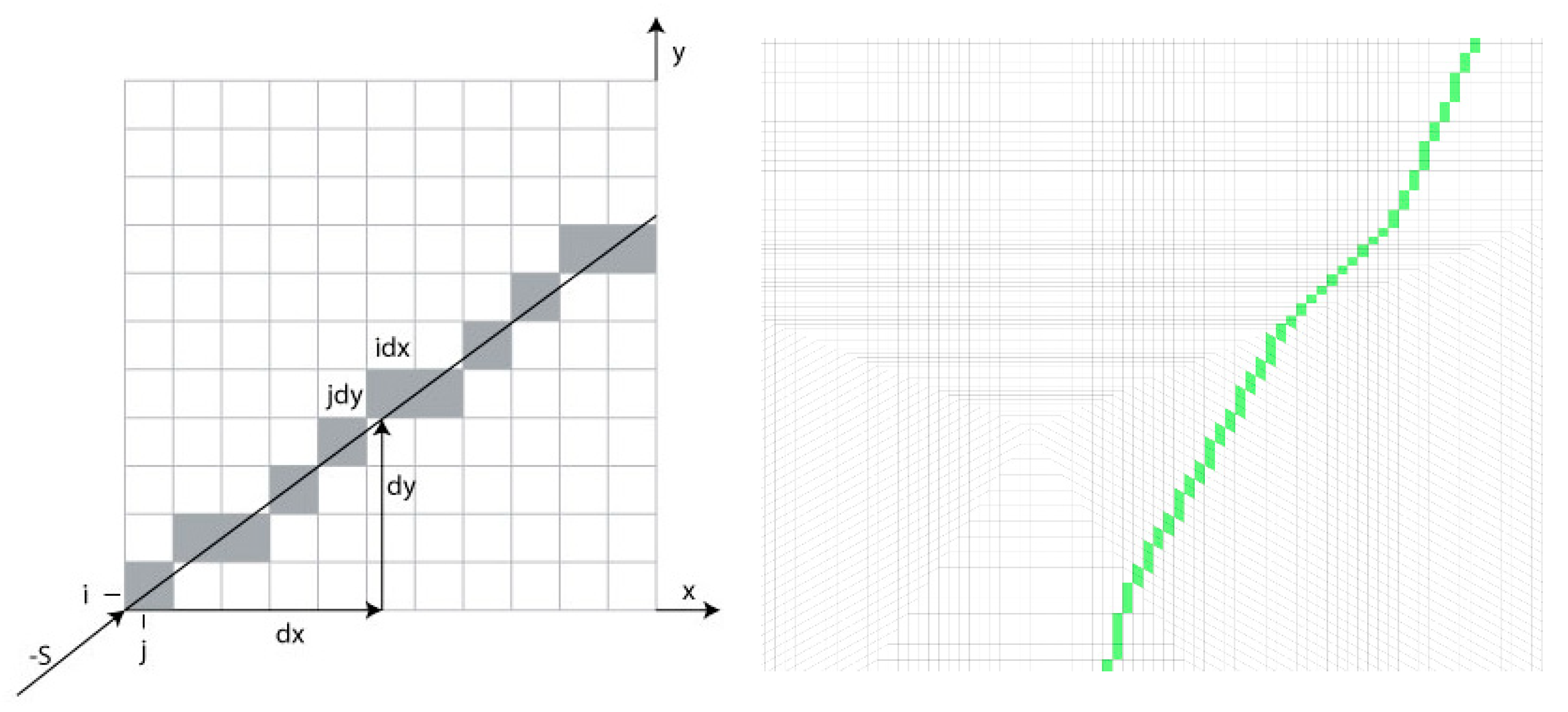
2.2.2. Determination of Cells on the Beam Path–Line Rasterization
2.2.3. Determination of Shadow Factor
The shadow factor can be determined on the basis of two known methods. The first approach (or vector method) presented in [38] determines the projection of individual cells on the plane Sp, which is perpendicular to the sun’s rays. The vector from the origin to any point Pi,j at column i, row j, can be calculated by Equation (8):
where li and lj stand for the cell sizes, and zi,j stands for the elevation of a cell at i, j. The plane, perpendicular to the Sun’s rays, is calculated as a combination of two cross products in Equation (9):
where s stands for solar vector and sxy0 stands for (XY) plane. The projection P′i,j of Pi,j is calculated by Equation (10):
The second approach (or geometrical method) presented in [38] determines whether the examined cell casts a shadow on the surrounding cells if the Sun’s rays are projected onto the model. The unit change of height μ for the solar vector s = [sx sy sz] is defined by Equation (11):
Using the change of height μ, when the solar vector s passes through the horizontal distance D between two given cells, a = [ax ay az] and b = [bx by bz], the height h can be determined by Equation (12):
The minimum height required to keep the cell out of the shade is hmin = ay − h. Otherwise, if the by < hmin, then cell b is shadowed by cell a [38]. The algorithm scans the entire model by the method described in Section 2.2.2. and determines for each cell a shadow factor sf, which is 0 for shaded cells and 1 for illuminated cells.
2.2.4. Determination of Geographic Potential Based on LiDAR Data
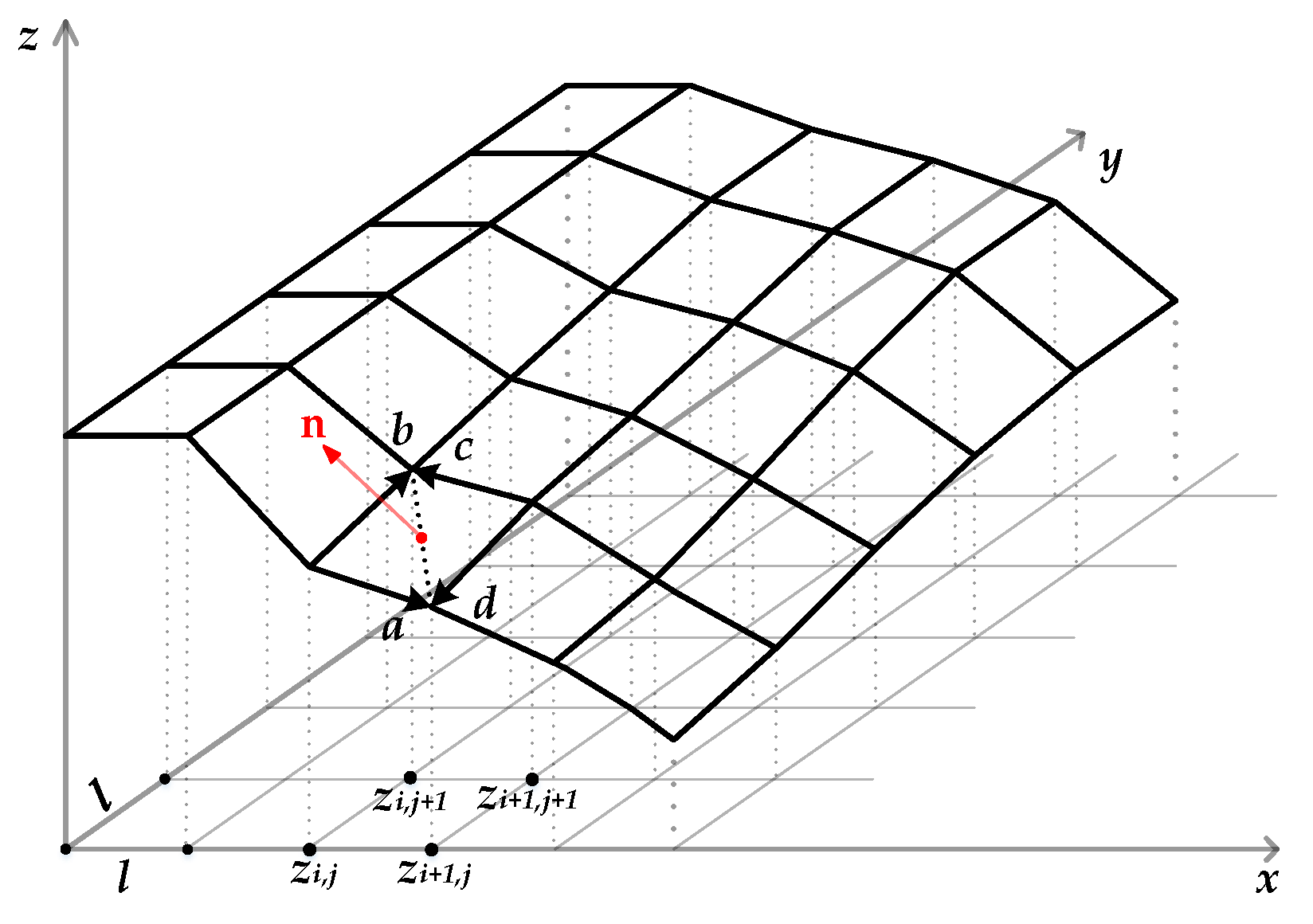
LiDAR data issued by the Slovenian Environment Agency [36] are in the ASCII format of cloud points located in the correct square network, where each point is defined by a coordinate in the 3-dimensional Cartesian coordinate system. To generate a surface model from LiDAR data, the plane enclosed by four data points zi,j, zi+1,j, zi,j+1, zi+1,j+1 must be determined, where zi,j is the elevation of points at row i, column j.
To calculate the geographic potential according to Equation (4), the algorithm must calculate the vector normal to the grid cell n, inclination β and azimuth angle γ of the cell. In a regular square grid of cell size l, the x, y, z components of the vectors along the side of the grid cell are defined by Equation (13) [36] and shown in Figure 6:
The vector normal to the surface is defined by half the sum of cross products of vectors along the sides of the grid cell in Equation (14):
By simplifying Equation (14), the components of the vector normal to the surface n can be written with the grid elevation points z and cell spacing l as Equation (15):
The inclination angle β and azimuth angle γ of the surface (cell) can be calculated from the component of the unit vector nu, as follows in Equations (16) and (17):
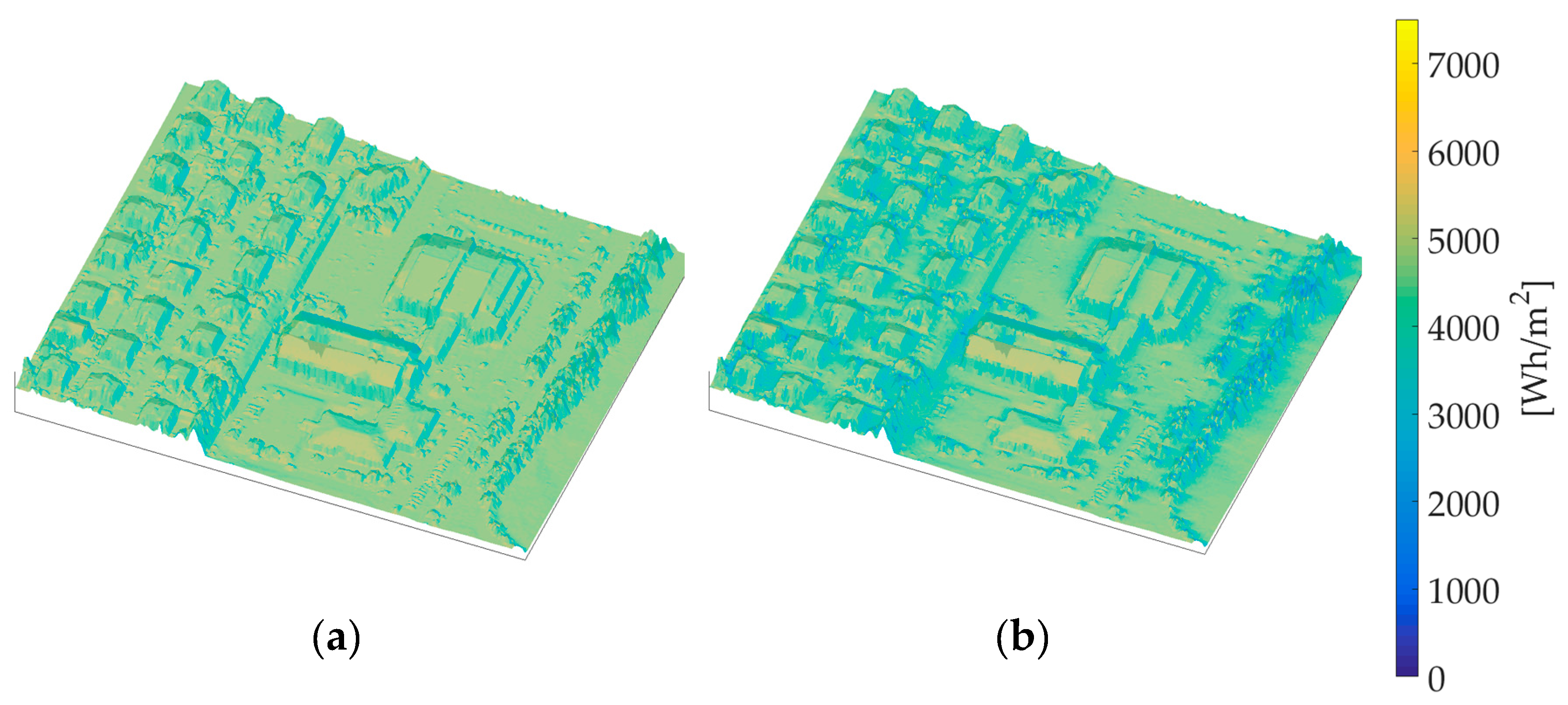
To determine the geographic potential that considers the shadowing effects of surroundings, the component of the solar radiation beam Gb(t) (described in Equation (4)) is multiplied by the shadow factor sf (described in Section 2.2.2), which determines whether or not the cells in the model are shaded. Therefore, the geographic potential can be calculated by Equation (18):
2.3. Technical Potential
The technical potential (TP) (Wh) presents the amount of energy that an available area with PV modules receives over a certain period of time, including the efficiency of the PV system. Technical potential can be calculated by Equation (19):
where ηPV stands for the efficiency of the PV module. To optimize the technical potential, the efficiency of the PV module can be calculated as a function of solar radiation G and temperature of the PV module T in three different ways, as shown in Equations (20)–(22) [39].
where G0 (1000 W/m2) and T0 (25 °C) stands for the solar radiation and temperature of the PV module under standard test conditions (STC). The parameters x1, x2, x3, x4, and x5 are determined by minimizing the root mean square error (RMSE) differences between measured and simulated values of the efficiency of the PV module.
2.4. Economic Potential
Economic potential EP (Wh) presents the amount of energy, taking into account technical potential, the price of electricity, the investment price, and the installed power of the PV system. The economic potential can be calculated by Equation (23):
where PRel stands for the price of electricity (€/Wh), PRPV stands for the price of the PV system (€/W), TP stands for technical potential (Wh), and PMPP stands for the installed power of the PV system. Other studies that also consider economic potential are extremely complicated and difficult to calculate, considering many different parameters that are often difficult to access, such as: building information (building characteristics, energy consumption, physical characteristics with spatial information), system size (maximum installation system size, eligible system size for policy implementation and 100% self-sufficiency), business model (self-consumption, power purchase agreement), etc. The new approach described in the paper offers a simplified model that still delivers accurate results and yet, makes it easier to calculate with easily accessible parameters such as: price of electricity, price of the PV system, installed power of the PV system and technical potential.
3. Results
In this section, the calculation of all potentials will be made on the rooftop of the Krško-Sevnica School Center (λ = 15°29′11″, φ = 45°56′42″), which is divided into 8 planes (see Figure 8). The required parameters for the calculation of different potentials are the total area of rooftop AT, the inclination angle β and the azimuth angle γ, which are described for each plane in Table 1.
3.1. Physical and Geographic Potential
The physical and geographic potentials were calculated for the period of one year, and Figure 9 shows the physical and geographic potentials (or hourly solar radiation on a horizontal surface) for an average day of the month. In Figure 9, the physical and geographic potentials for each month are presented in colored lines, according to the seasons, as (a) spring (green), (b) summer (orange), (c) autumn (yellow), and (d) winter (blue). First, the monthly values of physical and geographic potentials were the highest from 12 to 1 p.m., ranging from 185.5 to 826.6 kWh (for all months). Meanwhile, the monthly values of physical and geographic potentials were the lowest from 5 to 6 a.m., ranging from 6.552 to 73.584 kWh (from April to August). Second, in terms of seasons, physical and geographic potentials were the highest in July, May, September and February with monthly values of 417.9, 281.1, 220.9 and 104.9 MWh. The results from Figure 8 show that the deviation between physical and geographic potential is 1.56%, with annual physical potential of 1273.7 MWh and annual geographic potential of 1253.8 MWh. Figure 10 and Figure 11 show the geographic potential in graphical form for each month of the year, which also takes into account the shading effect. Figure 10 and Figure 11 shows which rooftops receive the highest amount of solar radiation and thus represent the optimal location for the installation of the PV system.
3.2. Technical Potential
The technical potential was calculated for the rooftop (Plane 1) for a period of one year (see Figure 8), on which a PV system with an installed power (PMPP) of 12.600 Wp is located. Measurement data was obtained from the owner of the PV system and included electrical quantities on the DC and AC sides of the inverter, air temperature, and solar radiation from a pyranometer mounted on the same inclination angle as the PV system modules [33]. To calculate the technical potential, the efficiency of the PV system was taken into account as a function of solar radiation G and temperature of the PV module T. The RMSE values of efficiency of the PV system (Table 2) show that the smallest RMSE is achieved by considering both solar radiation G and temperature of the PV module T in the calculation.
Therefore, Figure 12 presents the comparison between measured and modelled values of efficiency as a function of (a) solar radiation G, (b) temperature of PV module T, and (c) solar radiation G and temperature of PV module T. It can be seen that the efficiency of the PV system yields more accurate results if both solar radiation G and the temperature of PV module T are used in the calculation, as can be seen in Table 2. In Figure 13, the values of technical potential or generated electricity are presented for an average day of the month. First, the monthly values of technical potential were the highest from 12 to 1 p.m., ranging from 98.371 to 253.607 kWh (for all months). Meanwhile, the monthly values of technical potential were the lowest from 5 to 6 a.m., ranging from 0.0175 to 11.635 kWh (from April to August). Similar to the physical potential, the technical potential (in terms of seasons) was the highest in July, May, September and February with monthly values of 2197.8, 1511.1, 1280.5 and 588.3 kWh.
Figure 14 shows the comparison between technical potential and measurements of the PV system with an installed power of 12.6 kW. The results show that the deviation between measured values of generated electricity and technical potential is 3.45%, with annual measured generated electricity of 13.7 MWh and annual technical potential of 14.2 MWh.
3.3. Economic Potential
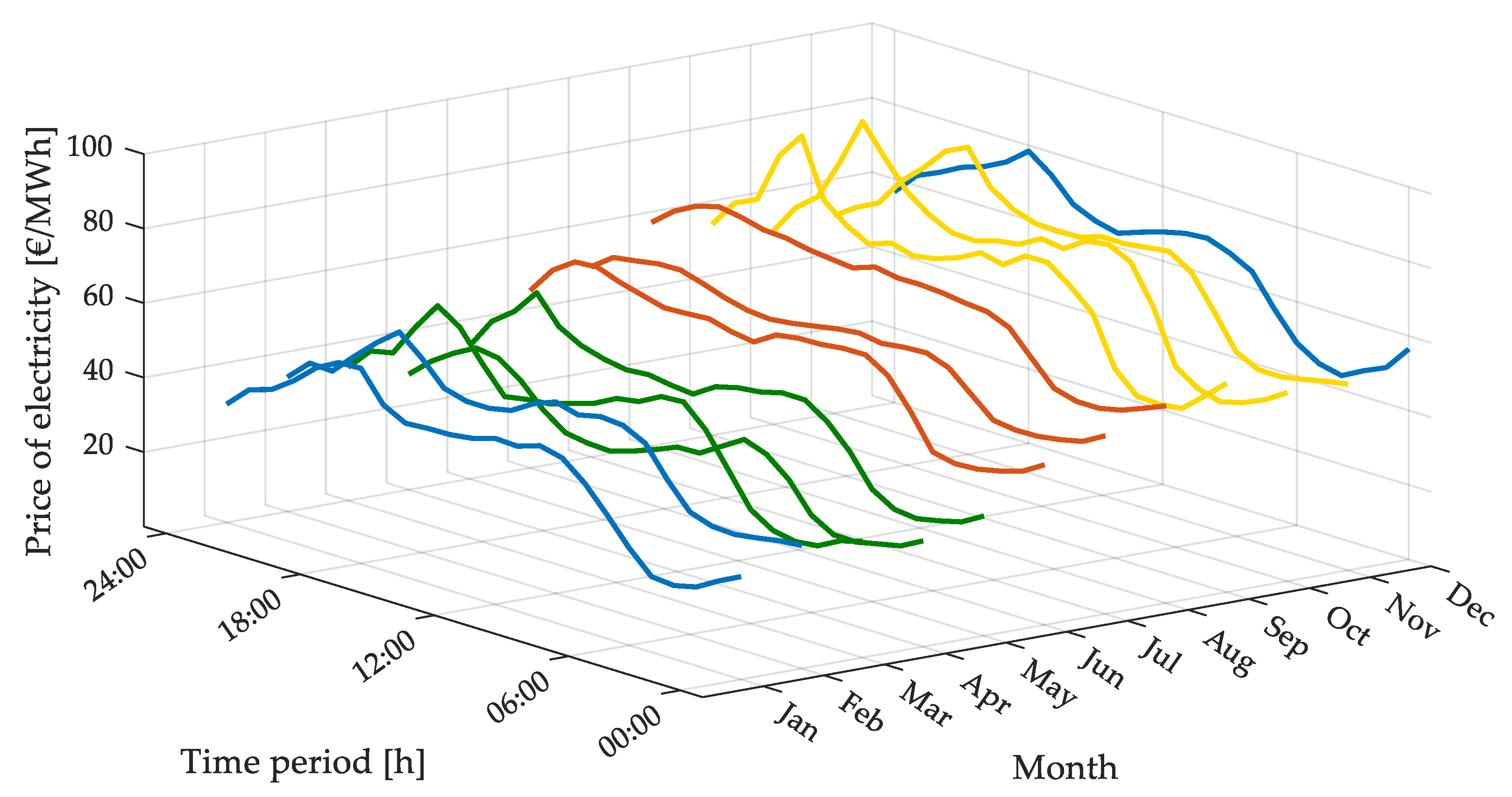
The economic potential was calculated based on the technical potential of the rooftop (Plane 1) and the variable price of electricity. Figure 15 presents the variable price of electricity throughout the day and year, showing that the price of electricity varies throughout every day of the year. Therefore, it is important to highlight in which part of the day electricity is the cheapest and most expensive. The lowest price for electricity is mainly at night (between midnight and 6 a.m.) and during working hours (between 11 a.m. and 4 p.m.), while the most expensive is in the morning (between 7 a.m. and 10 a.m.) and evening (between 5 p.m. and 10 p.m.). Furthermore, the price of electricity is the cheapest in January, February and April, while the most expensive is in September, October and November.
First, the monthly values of economic potential were the highest from 12 to 1 p.m., ranging from 1.22 to 8.41 Wh (for all months). However, in terms of seasons, the economic potential was slightly different from the technical potential, due to the impact of the price of electricity. In terms of physical, geographical and technical potential, the highest values first appeared in summer, spring, autumn and winter, while in economic potential, the highest values first appeared in summer (higher prices of electricity), autumn, spring and then winter. The economic potential was the highest in August, May, September and February with monthly values of 60.3, 29.87, 22.79 and 5.72 Wh.
The Slovenian electricity market is located at the intersection of three major European markets, the German-Austrian, Italian and Southeast European markets. There are several reasons for raising the average prices of base-load and peak energy in the market for the day ahead. Most important is the poor hydrology of the rivers and therefore, the relatively low production of electricity from hydropower plants. Economic growth and the growth of industrial production in EU countries also contributed to the rise in prices, which increased energy demand and is a consequence of the change in electricity prices shown in Figure 15. The price of the PV system PRPV was determined as the average value of all costs of the PV system in Slovenia (installation costs), which included: solar modules, installation, inverters, and documentation. Figure 16 shows the reflection of technical potential if specific economic parameters are taken into account. It can be seen that the most suitable months for the generation of electricity, regardless of the technical parameters, are the summer months. Indeed, during the summer months, the most substantial yield of solar radiation occurs, but this is also influenced by the medium-high cost of electricity.
3.4. Comparison of Physical, Geographic, Technical, and Economic Potentials
In this subsection, the comparison between physical, geographic, technical, and economic potentials is presented. Figure 16 shows the average monthly potentials of the rooftop in normalized values ranging from 0 to 1. As shown in Figure 9, Figure 13 and Figure 16, and especially in Figure 17, the monthly physical, geographic, and technical potentials had the increase of potential in spring and summer and decrease in fall and winter. It is evident that the most important role in determining the economic potential is played by the price of electricity, since in the summer and spring months the economic potential ranges between 0.7 and 1, and in the other months between 0 and 0.5. Overall, the annual physical, geographic, technical and economic potentials are 1273.7, 1253.8, 14.2 MWh and 279.1 Wh, respectively. As can be seen from Figure 17, the geographic and physical potentials are almost identical. In other studies, there is a major discrepancy between these two potentials. In our case, similarities occur because of the smaller surrounding objects and thus, the smaller influence of the shadow on the observed area. In other studies, [24], the difference between them is much larger, since the calculation is made on a much larger area, where the layout of the objects is much more diverse. The most important part of this study was the calculation of economic potential, as it will play a massive role in the near future.
4. Conclusions
This paper presents a simplified approach for estimating the rooftop solar potential. Apart from other studies presented in this paper, the estimation of rooftop solar potential is divided into the following four parts: (a) physical potential, (b) geographic potential, (c) technical potential, and (d) economic potential. In summary, based on the annual values of physical, geographic and technical potential, an analysis of the proportion by season was performed, which accounts for about 28%, 45%, 17% and 10% for spring, summer, fall and winter. The effects of different economic indicators and the dynamics of the stock market have a slightly different effect on the economic potential, since the share for the fall is approximately the same, while the share for the summer is 14% higher and 5% lower for the winter. The results presented in the paper show that the months from May to September are the most suitable months for Slovenia in terms of economic potential, which represents as much as 78% (3/4) of the annual economic potential, while the technical potential (and other potentials) have a more evenly distributed potential throughout the year. The message of this paper is that in the near future it will be necessary to take greater emphasis on the economic potential, than on the technical potential, when installing the PV systems, or in other words, less important will be the cumulative amount of annually produced electricity, and more significant will be the financial outflow. This may have a strategic impact on decision-making policies for the deployment of the PV systems in urban environments.
The new simplified approach differs from other studies by a simple but accurate calculation, since other studies are more complex and take into account more difficult-to-access information that is impossible to obtain for a larger urban area. The calculation takes into account the essential characteristics of the PV system and the dynamics of the electricity market, while other studies, in addition, place greater emphasis on the energy consumption by the consumer of the building on which the PV system is installed.
Author Contributions
For research articles with several authors, a short paragraph specifying their individual contributions must be provided. The following statements should be used “conceptualization, S.S. and P.M.; methodology, S.S.; software, P.M.; validation, K.S., S.S. and P.M.; formal analysis, S.S.; investigation, K.S.; resources, S.S.; data curation, P.M.; writing—original draft preparation, P.M.; writing—review and editing, K.S.; visualization, K.S.; supervision, B.Š. and M.H.; project administration, S.S.
Funding
This research received no external funding.
Conflicts of Interest
The authors declare no conflict of interest. The funders had no role in the design of the study; in the collection, analyses, or interpretation of data; in the writing of the manuscript, or in the decision to publish the results.
References
- Yuan, J.; Farnham, C.; Emura, K.; Lu, S. A method to estimate the potential of rooftop photovoltaic power generation for a region. Urban Clim. 2016, 17, 1–19. [Google Scholar] [CrossRef]
- Suomalainen, K.; Wang, V.; Sharp, B. Rooftop solar potential based on LiDAR data: Bottom-up assessment at neighbourhood level. Renew. Energy 2017, 111, 463–475. [Google Scholar] [CrossRef]
- Nadal, A.; Cadena, D.R.; Pons, O.; Cuerva, E.; Josa, A.; Rieradevall, J. Feasibility assessment of rooftop greenhouses in Latin America. The case study of a social neighborhood in Quito, Ecuador. Urban For. Urban Green. 2019, 44, 126389. [Google Scholar] [CrossRef]
- Rodríguez, L.R.; Duminil, E.; Ramos, J.S.; Eicker, U. Assessment of the photovoltaic potential at urban level based on 3D city models: A case study and new methodological approach. Sol. Energy 2017, 146, 264–275. [Google Scholar] [CrossRef]
- Bódis, K.; Kougias, I.; Jäger-Waldau, A.; Taylor, N.; Szabó, S. A high-resolution geospatial assessment of the rooftop solar photovoltaic potential in the European Union. Renew. Sustain. Energy Rev. 2019, 114, 10930. [Google Scholar] [CrossRef]
- Singh, R.; Asif, A.A.; Venayagamoorthy, G.K.; Lakhtakia, A.; Abdelhamid, M.; Alapatt, G.F.; Ladner, D.A. Emerging Role of Photovoltaics for Sustainably Powering Underdeveloped, Emerging, and Developed Economies. In Proceedings of the 2nd International Conference on Green Energy and Technology, Dhaka, Bangladesh, 5–6 September 2014; pp. 1–8. [Google Scholar]
- Buffat, R.; Grassi, S.; Raubal, M. A scalable method for estimating rooftop solar irradiation potential over large regions. Appl. Energy 2018, 216, 389–401. [Google Scholar] [CrossRef]
- Khan, J.; Arsalan, M.H. Estimation of rooftop solar photovoltaic potential using geo-spatial techniques: A perspective from planned neighborhood of Karachi–Pakistan. Renew. Energy 2016, 90, 188–203. [Google Scholar] [CrossRef]
- Assouline, D.; Mohajeri, N.; Scartezzini, J.L. Quantifying rooftop photovoltaic solar energy potential: A machine learning approach. Sol. Energy 2017, 141, 278–296. [Google Scholar] [CrossRef]
- Saha, M.; Eckelman, M.J. Growing fresh fruits and vegetables in an urban landscape: A geospatial assessment of ground level and rooftop urban agriculture potential in Boston, USA. Landsc. Urban Plan. 2017, 165, 130–141. [Google Scholar] [CrossRef]
- Ko, L.; Wang, J.C.; Chen, C.Y.; Tsai, H.Y. Evaluation of the development potential of rooftop solar photovoltaic in Taiwan. Renew. Energy 2015, 76, 582–595. [Google Scholar] [CrossRef]
- Byrne, J.; Taminiau, J.; Kurdgelashvili, L.; Kim, K.N. A review of the solar city concept and methods to assess rooftop solar electric potential, with an illustrative application to the city of Seoul. Renew. Sustain. Energy Rev. 2015, 41, 830–844. [Google Scholar] [CrossRef]
- Takebayashi, H.; Ishii, E.; Moriyama, M.; Sakaki, A.; Nakajima, S.; Ueda, H.H. Study to examine the potential for solar energy utilization based on the relationship between urban morphology and solar radiation gain on building rooftops and wall surfaces. Sol. Energy 2015, 119, 362–369. [Google Scholar] [CrossRef]
- Peng, J.; Lu, L. Investigation on the development potential of rooftop PV system in Hong Kong and its environmental benefits. Renew. Sustain. Energy Rev. 2013, 27, 149–162. [Google Scholar] [CrossRef]
- Song, X.; Huang, Y.; Zhao, C.; Liu, Y.; Lu, Y.; Chang, Y.; Yang, J. An Approach for Estimating Solar Photovoltaic Potential Based on Rooftop Retrieval from Remote Sensing Images. Energies 2018, 11, 3172. [Google Scholar] [CrossRef]
- Odeh, S. Thermal Performance of Dwellings with Rooftop PV Panels and PV/Thermal Collectors. Energies 2018, 11, 1879. [Google Scholar] [CrossRef]
- Melius, J.; Margolis, R.; Ong, S. Estimating Rooftop Suitability for PV: A Review of Methods, Patents, and Validation Techniques; Technical Report NREL/TP-6A20-60593; National Renewable Energy Lab.: Golden, CO, USA, 2013. [Google Scholar]
- Palmer, D.; Koumpli, E.; Cole, I.; Gottschalg, R.; Betts, T. A GIS-Based Method for Identification of Wide Area Rooftop Suitability for Minimum Size PV Systems Using LiDAR Data and Photogrammetry. Energies 2018, 11, 3506. [Google Scholar] [CrossRef]
- Assouline, D.; Mohajeri, N.; Scartezzini, J.L. Large-scale rooftop solar photovoltaic technical potential estimation using Random Forests. Appl. Energy 2018, 217, 189–211. [Google Scholar] [CrossRef]
- Kurdgelashvili, L.; Li, J.; Shih, C.H.; Attia, B. Estimating technical potential for rooftop photovoltaics in California, Arizona and New Jersey. Renew. Energy 2016, 95, 286–302. [Google Scholar] [CrossRef] [Green Version]
- Lee, M.; Hong, T.; Jeong, J.; Jeong, K. Development of a rooftop solar photovoltaic rating system considering the technical and economic suitability criteria at the building level. Energy 2018, 160, 213–224. [Google Scholar] [CrossRef]
- Miranda, R.F.C.; Szklo, A.; Schaeffer, R. Technical-economic potential of PV systems on Brazilian rooftops. Renew. Energy 2015, 75, 694–713. [Google Scholar] [CrossRef]
- Xin-gang, Z.; Yi-min, X. The economic performance of industrial and commercial rooftop photovoltaic in China. Energy 2019, 187, 115961. [Google Scholar] [CrossRef]
- Hong, T.; Lee, M.; Koo, C.; Jeong, K.; Kim, J. Development of a method for estimating the rooftop solar photovoltaic (PV) potential by analyzing the available rooftop area using Hillshade analysis. Appl. Energy 2017, 194, 320–332. [Google Scholar] [CrossRef]
- Lee, M.; Hong, T.; Jeong, K.; Kim, J. A bottom-up approach for estimating the economic potential of the rooftop solar photovoltaic system considering the spatial and temporal diversity. Appl. Energy 2018, 232, 640–656. [Google Scholar] [CrossRef]
- Deline, C. Partially shaded operation of a grid-tied PV system. In Proceedings of the 34th IEEE Photovoltaic Specialists Conference (PVSC), Philadelphia, PA, USA, 7–12 June 2009; pp. 1268–1273. [Google Scholar]
- Woyte, A.; Nijs, J.; Belmans, R. Partial shadowing of photovoltaic arrays with different system configurations: Literature review and field test results. Sol. Energy 2003, 74, 217–233. [Google Scholar] [CrossRef]
- García, M.; Maruri, J.M.; Marroyo, L.; Lorenzo, E.; Pérez, M. Partial shadowing, MPPT performance and inverter configurations: Observations at tracking PV plants. Prog. Photovolt. Res. Appl. 2008, 16, 529–536. [Google Scholar] [CrossRef]
- Ahmad, R.; Murtaza, A.F.; Sher, H.A.; Shami, U.T.; Olalekan, S. An analytical approach to study partial shading effects on PV array supported by literature. Renew. Sustain. Energy Rev. 2017, 74, 721–732. [Google Scholar] [CrossRef]
- Malathy, S.; Ramaprabha, R. Reconfiguration strategies to extract maximum power from photovoltaic array under partially shaded conditions. Renew. Sustain. Energy Rev. 2018, 81, 2922–2934. [Google Scholar] [CrossRef]
- Lukač, N.; Žalik, B. GPU-based roofs’ solar potential estimation using LiDAR data. Comput. Geosci. 2013, 52, 34–41. [Google Scholar] [CrossRef]
- Lukač, N.; Žlaus, D.; Seme, S.; Žalik, B.; Štumberger, G. Rating of roofs’ surfaces regarding their solar potential and suitability for PV systems, based on LiDAR data. Appl. Energy 2013, 102, 803–812. [Google Scholar] [CrossRef]
- Seme, S.; Požun, J.; Štumberger, B.; Hadžiselimović, M. Energy Production of Different Types and Orientations of Photovoltaic Systems Under Outdoor Conditions. J. Sol. Energy Eng. 2015, 137, 021021. [Google Scholar] [CrossRef]
- Jacques, D.A.; Gooding, J.; Giesekam, J.J.; Tomlin, A.S.; Crook, R. Methodology for the assessment of PV capacity over a city region using low-resolution LiDAR data and application to the City of Leeds (UK). Appl. Energy 2014, 124, 28–34. [Google Scholar] [CrossRef]
- Maciejowska, K.; Nitka, W.; Weron, T. Day-Ahead vs. Intraday—Forecasting the Price Spread to Maximize Economic Benefits. Energies 2019, 12, 631. [Google Scholar] [CrossRef]
- Slovenian Environmental Agency. Official Website. 2017. Available online: http://www.arso.gov.si/ (accessed on 10 September 2019).
- Liu, B.Y.H.; Jordan, R.C. Daily insolation on surfaces tilted towards the equator. ASHRAE J. 1961, 3, 53–59. [Google Scholar]
- Corripio, J.G. Vectorial algebra algorithms for calculating terrain parameters from DEMs and solar radiation modelling in mountainous terrain. Int. J. Geogr. Inf. Sci. 2003, 17, 1–23. [Google Scholar] [CrossRef]
- Durisch, W.; Bitnar, B.; Mayor, J.C.; Kiess, H.; Lam, K.; Close, J. Efficiency model for photovoltaic modules ad demonstration of its application to energy yield estimation. Sol. Energy Mater. Sol. Cells 2007, 91, 79–84. [Google Scholar] [CrossRef]
Figure 1.
Hierarchical distribution of physical, geographic, technical and economic potentials. PV = photovoltaic.
Figure 1.
Hierarchical distribution of physical, geographic, technical and economic potentials. PV = photovoltaic.

Figure 2.
Location of the photovoltaic system Krško-Sevnica School Center, Slovenia.

Figure 3.
Visualization of the method for analyzing the availability of rooftop PV potential: (a) Physical potential; (b) Geographic potential; (c) Technical potential; (d) Economic potential.
Figure 3.
Visualization of the method for analyzing the availability of rooftop PV potential: (a) Physical potential; (b) Geographic potential; (c) Technical potential; (d) Economic potential.

Figure 4.
Rotation of the topo-centric coordinate system XYZ at angle ω, from time t0 to time t1 [37].
Figure 4.
Rotation of the topo-centric coordinate system XYZ at angle ω, from time t0 to time t1 [37].

Figure 5.
Determination of cells on the beam path.

Figure 6.
Vector normal to the grid cell surface.

Figure 7.
Geographic potential without (a) or with (b) shadowing effects of surroundings.

Figure 8.
Visualization of the rooftop divided into 8 planes (colors in image present relative altitude).
Figure 8.
Visualization of the rooftop divided into 8 planes (colors in image present relative altitude).

Figure 9.
Results of the physical and geographic potential for the rooftops of the Krško-Sevnica School Center.
Figure 9.
Results of the physical and geographic potential for the rooftops of the Krško-Sevnica School Center.

Figure 10.
Visualization of the geographic potential for January, February, March, April, May and June.
Figure 10.
Visualization of the geographic potential for January, February, March, April, May and June.

Figure 11.
Visualization of the geographic potential for July, August, September, October, November and December.
Figure 11.
Visualization of the geographic potential for July, August, September, October, November and December.

Figure 12.
Comparison between measured and modelled values of efficiency as a function of (a) solar radiation G, (b) temperature of PV module T, and (c) solar radiation G and temperature of PV module T.
Figure 12.
Comparison between measured and modelled values of efficiency as a function of (a) solar radiation G, (b) temperature of PV module T, and (c) solar radiation G and temperature of PV module T.

Figure 13.
Results of the technical potential for the rooftops of the Krško-Sevnica School Center.

Figure 14.
Comparison between technical potential and measurements.

Figure 15.
Price of electricity for the average day of the month in 2018.

Figure 16.
Results of the economic potential for the rooftops of the Krško-Sevnica School Center.

Figure 17.
Results of the comparison between physical, geographic, technical and economic potentials for the rooftops of the Krško-Sevnica School Center.
Figure 17.
Results of the comparison between physical, geographic, technical and economic potentials for the rooftops of the Krško-Sevnica School Center.


Table 1.
Rooftop parameters.
| Parameters | Plane 1 | Plane 2 | Plane 3 | Plane 4 | Plane 5 | Plane 6 | Plane 7 | Plane 8 |
|---|---|---|---|---|---|---|---|---|
| AT [m2] | 224 | 91 | 215 | 80 | 177 | 58 | 51 | 112 |
| β [°] | 15 | 15 | 15 | 15 | 15 | 15 | 15 | 15 |
| γ [°] | 0 | 90 | −180 | −90 | 90 | −180 | 0 | −90 |
Table 2.
RMSE values of efficiency of the PV system.
| Equation | Parameters | ||||||
|---|---|---|---|---|---|---|---|
| x1 | x2 | x3 | x4 | x5 | RMSE | ||
| Equation (20) | η(G) | 0.0568 | −0.4678 | 0.2368 | −2.7297 | 4.1496 | 2.0727 |
| Equation (21) | η(T) | −0.0732 | −1.7987 | / | −0.0925 | 0.1063 | 3.0412 |
| Equation (22) | η(G,T) | 0.1235 | −0.4544 | 0.2420 | −0.0309 | −0.3854 | 2.0217 |
© 2019 by the authors. Licensee MDPI, Basel, Switzerland. This article is an open access article distributed under the terms and conditions of the Creative Commons Attribution (CC BY) license (http://creativecommons.org/licenses/by/4.0/).
Share and Cite
MDPI and ACS Style
Mavsar, P.; Sredenšek, K.; Štumberger, B.; Hadžiselimović, M.; Seme, S. Simplified Method for Analyzing the Availability of Rooftop Photovoltaic Potential. Energies 2019, 12, 4233. https://doi.org/10.3390/en12224233
AMA Style
Mavsar P, Sredenšek K, Štumberger B, Hadžiselimović M, Seme S. Simplified Method for Analyzing the Availability of Rooftop Photovoltaic Potential. Energies. 2019; 12(22):4233. https://doi.org/10.3390/en12224233
Chicago/Turabian StyleMavsar, Primož, Klemen Sredenšek, Bojan Štumberger, Miralem Hadžiselimović, and Sebastijan Seme. 2019. "Simplified Method for Analyzing the Availability of Rooftop Photovoltaic Potential" Energies 12, no. 22: 4233. https://doi.org/10.3390/en12224233
Note that from the first issue of 2016, this journal uses article numbers instead of page numbers. See further details here.