Functional Equations for Calculating the Properties of Low-GWP R1234ze(E) Refrigerant


Department of Environmental Engineering, AGH University of Science and Technology, 30-059 Krakow, Poland
*
Author to whom correspondence should be addressed.
Energies 2020, 13(12), 3052; https://doi.org/10.3390/en13123052
Submission received: 10 May 2020
/
Revised: 9 June 2020
/
Accepted: 10 June 2020
/
Published: 12 June 2020
(This article belongs to the Special Issue Refrigeration Systems and Applications 2020)
Abstract
:Legal requirements for the use of refrigerants increasingly restrict the use of high-global warming potential (GWP) refrigerants. As a result, there is a growing interest in natural refrigerants and in those belonging to the hydrofluoroolefins (HFO) class, which can be used on their own or in mixtures. One of them is the R1234ze(E) refrigerant, an alternative to the R134a refrigerant as well as being a component of numerous mixtures. The knowledge of thermodynamic and transport properties of refrigerants is required for the analysis and calculation of refrigeration cycles in refrigeration, air conditioning, or heating systems. The paper presents analytical equations for calculating the properties of the R1234ze(E) refrigerant in the state of saturation and in the subcooled liquid and superheated vapour regions that do not require numerical calculations and are characterised by small deviations. The Levenberg–Marquardt algorithm—one of the methods for non-linear least squares estimation—was used to develop them. A total of 26 equations were formulated. The formulated equations were statistically verified by determining absolute and relative deviations between the values obtained from CoolProp software and calculated values. The maximum relative deviation was not higher than 1% in any of them.
1. Introduction
The restrictions against the use of many refrigerants in the UE due to their high global warning potential (GWP) values have been in force since 1 January 2015 [1]. Gradually reducing the quantities of fluorinated greenhouse gases that can be placed on the market has been identified as an effective way to reduce the emissions of these substances in the long term. Regulation (EU) No 517/2014 of the European Parliament and the Council that came into place on 16 April 2014 regulates fluorinated greenhouse gases and repealing Regulation (EC) No 842/2006 sets out the quantity and phase down timetable of hydrofluorocarbons (HFC) based on tonnes of CO2 equivalent, taking 2015 as the reference year. These not only refer to high-GWP HFC refrigerants but also refer to mixtures containing these substances and other fluorinated greenhouse gases.
Legal requirements concerning high-GWP refrigerants have forced the industry to seek substitutes with the lowest GWP values. This is particularly important in the case of refrigerants that are frequently used in the refrigeration or heating industries such as R134a, R404A, R407C, R410A, and R507A. According to European Environment Agency data [2], the total supply of HFC refrigerants was 87,533 tonnes in the EU in 2017. Fifty percent of the total supply concerned R134a, while 21%, 15%, and 7% concerned R125, R32, and R143a, respectively. All of these refrigerants are used on their own or in the popular mixtures R404A, R407C, R410A, and R507A. The use of substitutes mainly depends on how they are used (drop-in, retrofit) and on their required properties such as flammability, toxicity, performance, efficiency, and working pressure. Therefore, these refrigerants cannot be directly substituted for a single universal refrigerant to be used in all applications. It appears that the majority of substitutes are highly flammable (e.g., R600a, R290, R1270), toxic (e.g., R717), have a high working pressure or sometimes have several of such properties at the same time.
One of the substitutes for high-GWP refrigerants currently in use is the R1234ze(E) refrigerant belonging to the hydrofluoroolefins (HFO) class, which is an alternative to the widely used high-GWP R134a refrigerant (GWP100 = 1300). Generally, this refrigerant is used for high- and medium-temperature refrigeration and air conditioning applications for both low- (several kW) and high-power (several dozen MW) units. The R1234ze(E) refrigerant has a very low GWP value (GWP100 = 1) but is also mildly flammable (A2L rating). The basic thermodynamic properties of the R1234ze(E) refrigerant are given in Table 1.
Many studies have performed theoretical analyses and experimental research on the use of the R1234ze(E) refrigerant. A comparative analysis of R1234yf and R1234ze(E) refrigerants as substitutes for the R134a refrigerant in small air conditioning units was presented in [5]. Drop-in tests revealed that in the case of R1234ze(E), a larger compressor is required to achieve a comparable performance to R134a. This is due to a higher pressure drop in the system. The use of R1234yf and R1234ze(E) refrigerants instead of the R134a refrigerant in the Organic Rankine Cycle (ORC) was presented in [6]. Theoretical analyses showed that the R1234ze(E) refrigerant requires 15.7–20.2% less pumping power and achieves a net cycle efficiency of up to 13.8% higher than that of R134a in the range of the analysed operating conditions. The same substitutes were examined in terms of the use of an internal heat exchanger in the study [7]. The R1234ze(E) refrigerant had a lower cooling capacity and energy consumption but a higher coefficient of performance (COP). In addition, the use of an internal heat exchanger in the cycle with R1234ze(E) increased the COP by 3% compared to the cycle with R1234ze(E) without an internal heat exchanger. The same authors [8] presented a theoretical analysis of the use of R1234yf, R1234ze(E), R513A, R445A, and R450A refrigerants as substitutes for the R134a refrigerant for three refrigeration systems (basic, basic with an internal heat exchanger, and cascade). The calculations showed similar behaviours for all substitutes, but the R450A refrigerant had the closest COP (COP = 3.83) to the R134a refrigerant (COP = 3.86). When flammability was excluded as a property that determines application, the R445A refrigerant had the best results (COP = 4.10). The COP for R1234ze(E) was slightly smaller (COP = 3.85) than that for R134a. Furthermore, the use of an internal heat exchanger improved performance of all analysed replacements. A model study on the replacement of the R134a refrigerant with the R1234ze(E) refrigerant in water cooling units was published in [9]. The effects of the ambient temperature and evaporation temperature on the capacity of a cooling unit were analysed. The results revealed similar energy efficiency values. The behaviour of R1234yf and R1234ze(E) refrigerants as drop-in substitutes in a low-power refrigeration system was analysed in [10]. The developed mathematical model of the refrigeration system revealed, in particular, that assuming the same evaporation and condensation temperatures, the system cooling capacity of the R1234yf and R1234ze(E) refrigerants is lower than that for the R134a refrigerant (by 6% and 27% respectively). COPs were found to be approx. 1% smaller for R1234yf and 2–5% for R1234ze(E). The authors concluded that R1234yf seems to be the right substitute for R134a, while R1234ze(E) can obtain better operating parameters if changes are made to the compressor. The effects of using an internal heat exchanger (IHX) in refrigeration systems after replacing the R134a refrigerant with R1234ze(E) and R450A refrigerants using the drop-in method were presented in [11]. IHX was shown to have a positive impact on the energy efficiency of all refrigerants tested. The increase in the COP of R1234ze(E) was the highest among all refrigerants tested. An extensive study of potential R134a substitutes was carried out in [12]. The R290, R600a, R152a, R1234yf, and R1234ze(E) refrigerants were examined. Replacing the R134a refrigerant with the R1234ze(E) refrigerant using the drop-in method led to noticeable reductions in the cooling capacity and energy consumption by 24.9% and 17.8%, respectively. As a result, the COP went down by approx. 8.6%. To obtain a cooling capacity comparable to the one obtained by the R134a refrigerant, the use of a compressor with a higher cylinder capacity is required. In a theoretical study, the R1234ze(E) refrigerant, as well as the R152a and R152a and R1234ze(E) mixtures, were analysed as substitutes for R134a in different ratios [13]. It was shown that R152a has a higher COP with an almost identical cooling capacity but a higher compression temperature and flammability. R1234ze(E) was shown to have a similar COP but a lower cooling capacity. In the view of the authors, the best drop-in substitute is the R152a/R1234ze(E) mixture in a 50:50 ratio. The COP was found to be 2% higher than the COP of R134a for a condensation temperature of 45 °C and 5% higher for a condensation temperature of 65 °C, but the cooling capacity was shown to be approx. 7% lower. In [14], a study on a window air conditioner, the R410A refrigerant was replaced with R32, the R32/R125 mixture, and with R600a, R290, R1234yf, R1234ze, and R134a. As far as the capacity was concerned, the best results were obtained with the R32 refrigerant (a 4% COP increase). The worst results were achieved by HFO refrigerants, i.e., R1234yf and R1234ze(E). A compressor with a higher cylinder capacity is required in order to obtain the same cooling capacity as R410A.
A detailed analysis of the properties of the R1234ze(E) refrigerant clearly indicated that it is a medium-pressure refrigerant, and it has been proposed as an alternative to R134a in new systems. It is not recommended as a drop-in or retrofit substitute for R134a due to the differences in its thermophysical properties [15].
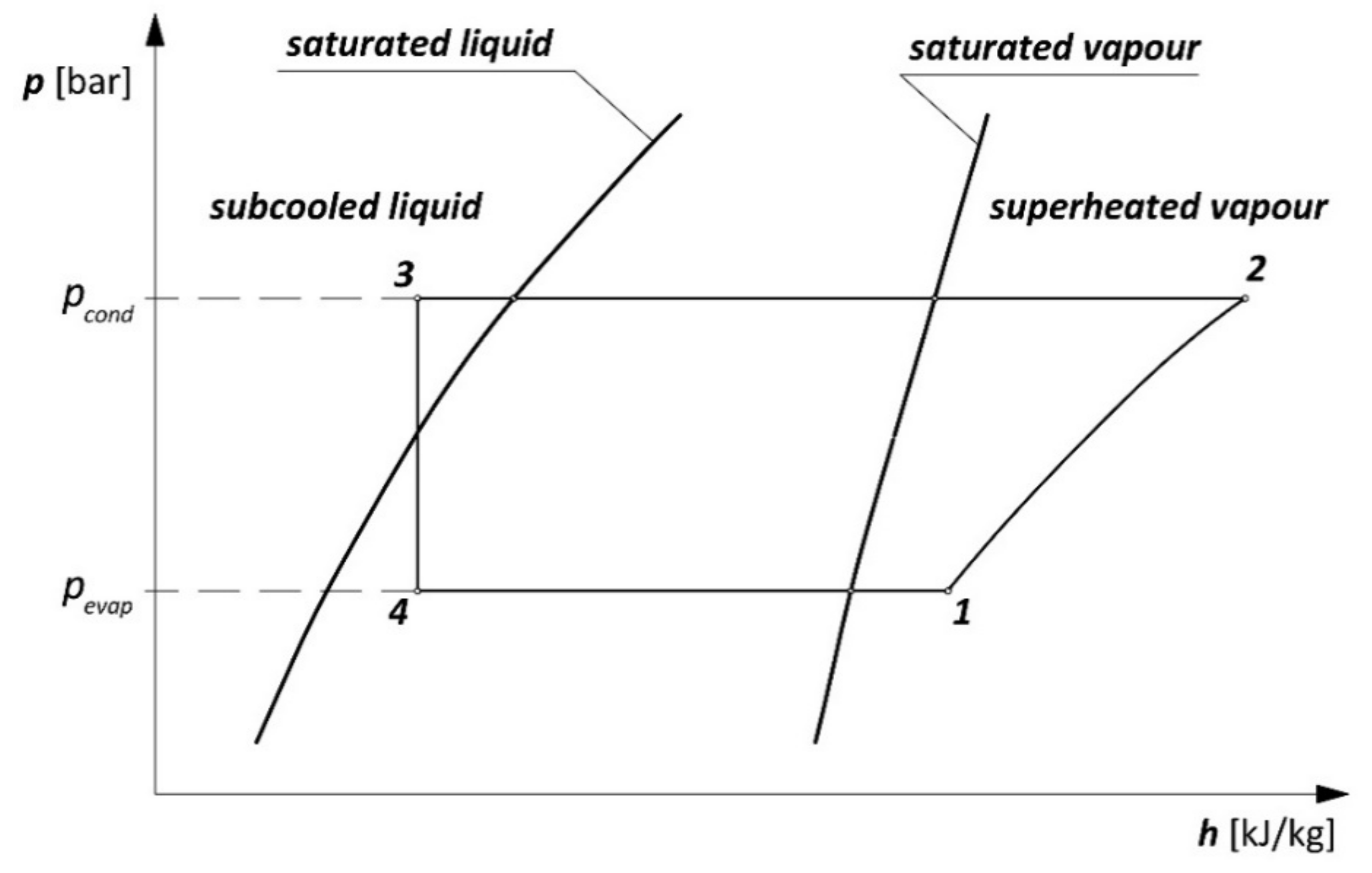
The R1234ze(E) refrigerant may be used not only as an alternative to R134a, but it can also be used as a component of mixtures substituting other refrigerants. It is a component of various refrigerants such as R444A, R444B, R445A, R447A, R448A, R450A, and R459B. The thermodynamic and thermokinetic properties of a refrigerant have to be known in order to carry out any analyses of its behaviour in a mixture, to determine the operating parameters of a refrigeration system, or to perform comparative analyses of the uses of different refrigerants. When it comes to analyses of refrigeration cycles (Figure 1), it is necessary to know the properties of a refrigerant in the subcooled liquid, saturated liquid, superheated vapour, and saturated vapour regions.
2. Modelling the Thermodynamic and Thermokinetic Properties of Refrigerants
Currently, computer databases containing detailed data on many liquids and mixtures are most often used to determine the properties of refrigerants. The most popular include REFPROP 10 [16] and CoolProp 6.3.0 [17]. These programmes and numerical calculations use various types of equations of state to describe relationships between individual properties, e.g., the ideal gas law, the Martin–Hou equation of state, the Redlich–Kwong equation of state, the Benedict–Webb–Rubin equation, and the Gibbs–Helmholtz equation, the last one being the most commonly used these days [18]. A detailed literature review of experimental data on thermophysical properties of low-GWP refrigerants that are necessary to formulate accurate equations of state was presented in [19].
For engineering calculations, equations describing refrigerant properties in a form that does not require numerical calculations are easier to use. Most of them, however, only refer to properties in the saturation state. In addition, their form is often complicated, while their scope is limited. Deviations from the source data are important when using such equations.
In [20], the Martin–Hou equation of state was applied to formulate equations that describe the thermodynamic properties of R407C and R410A refrigerants in the superheated vapour region. The equations are functions of the refrigerant-specific volume and temperature. F. de Monte [21] compared the calculation results obtained from the aforementioned equations with calculations obtained in the REFPROP programme. The calculation results of the thermodynamic properties of the R32, R125, and R134a refrigerants and their mixtures obtained from the General Cubic Equation of State with three Constant equations, the Soave modification of the Redlich–Kwong equation of state, and the Peng–Robinson equation of state are shown in [22,23]. G. Ding et al. [24] applied implicit curve fitting to determine equations describing the thermodynamic properties of the R22 and R407C refrigerants. The calculation formulas are valid not only for the subcooled liquid region but also for the wet and superheated vapour regions and in the state of saturation.
Equations that allow the specific volume, enthalpy, entropy, dynamic viscosity coefficient, and heat transfer coefficient of the R407C refrigerant to be calculated in the wet vapour and superheated vapour states are presented in [25]. To formulate equations, the authors used Artificial Neural Network (ANN) techniques. The same method was used in order to formulate equations describing the enthalpy and entropy of the wet vapour region and the enthalpy, entropy, and specific volume for superheated vapour for the R404A refrigerant [26]. To perform the formulated equations, the temperature and vapour quality of the refrigerant in the wet vapour state are required, while the temperature and pressure for the refrigerant are required in the superheated vapour state. To the determine the thermodynamic properties (enthalpy, entropy, specific volume) of the saturated liquid and saturated vapour of the R413A, R417A, R422A, R422D, and R423A refrigerants, the ANN method and the Adaptive Neuro-Fuzzy Inference System (ANFIS) were used [27]. The ANFIS model was proven to be more suitable for assessing the thermodynamic properties of refrigerants than the ANN model. Artificial neural networks were also applied to determine calculation formulas (enthalpy, entropy, specific volume of saturated liquid and saturated vapour) for natural refrigerants such as butane (R600), ethane (R170), methane (R50), and propane (R290) [28].
The properties of refrigerants (R12, R22, R134a, R209, R717 and R410a) using ANN were also presented in [29]. Equations used to determine the enthalpy, entropy, specific volume, specific heat, dynamic viscosity coefficient, heat transfer coefficient, and density of the R134a, R404a, R407C, and R410A refrigerants in the state of saturation are presented in [30,31]. The authors used different data mining techniques using WEKA software and presented a comparison of these modelling techniques. For example, the best approaches for entropy related to the liquid phase are the M5′Rules model for R134a, the multi-layer perception (MLP) model for R404a, the Pace regression (PR) model for R407C, and the MLP model for R410A. In contrast to equations presented in this paper, the limitation to the use of these equations is that knowledge of two properties of a refrigerant in the state of saturation—temperature and pressure—is required. In addition, the equations only apply to the saturation state.
Equations for fast calculations of the thermodynamic properties of refrigerants are presented in [32]. The authors present examples of equations that are used to calculate properties in the state of saturation based on having one different refrigerant property in the state of saturation and the temperature, specific enthalpy, entropy, and volume for pressure as well as on an additional property for superheated and wet vapours of R407C and R1234yf refrigerants. The authors developed explicit formulas based on implicit equations. The coefficients of the implicit equations were determined by curve-fitting methods (using implicit polynomial equations of order three).
This paper reveals analytical equations that can be used to determine the properties of the R1234ze(E) refrigerant for the state of saturation, subcooled liquid, and superheated vapour. Correlations for the calculations are a function of one variable for the state of saturation and two variables for the subcooled liquid and superheated vapour regions.
3. Correlations for Calculating the Thermodynamic and Thermokinetic Properties of the R1234ze(E) Refrigerant
To clearly determine the thermodynamic and thermokinetic properties of the refrigerant, knowledge of one independent variable (saturated liquid, saturated vapour) or two independent variables (superheated vapour, subcooled liquid, wet saturated vapour) is required.
The input and output data of the R1234ze(E) refrigerant required for analysis were obtained from the CoolProp 5.1.1 programme [17]. The sought-after thermodynamic and thermokinetic properties were described using 3, 4, 5, 6, 8, or 9 degree polynomials, whose coefficients were determined using STATISTICA 12 [33]. As in [34,35,36,37], the Levenberg–Marquardt algorithm—one of the methods used for non-linear least squares estimation—was used for this purpose. The Levenberg–Marquardt algorithm is used directly or indirectly in many technology fields, such as energy flow research [38], heat transfer [39,40], PV module parameters [41,42], and water flow [43].
The scope of individual equations and the amount of data analysed depending on the state of the refrigerant are given in Table 2.
3.1. Saturated Liquid Region
For the R1234ze(E) refrigerant in the saturated liquid state, equations describing the following basic thermodynamic and thermokinetic properties as a function of pressure were formulated: temperature T [K], specific enthalpy h′ [kJ/kg], specific entropy s′ [kJ/(kg·K)], specific heat cp′ [kJ/(kg·K)], density ρ′ [kg/m3], specific volume ν′ [m3/kg], heat transfer coefficient λ′ [W/(m·K)], dynamic viscosity coefficient µ′ [kg/(m·s)], Prandtl number Pr′ [-], and surface tension σ [N/m]. Using CoolProp 5.1.1, the values of corresponding saturated liquid properties were determined for pressure in the range of 0.5–30 bar changing by 0.05 bar. To make the calculations, a total of 591 pieces of data were used for each refrigerant property analysed. Equations for the R1234ze(E) refrigerant in the state of saturated liquid were as follows:
The polynomial coefficients determined for the individual properties of the refrigerant are given in Table 3 (temperature, specific enthalpy, specific entropy, specific heat), Table 4 (density, specific volume, heat transfer coefficient), and Table 5 (dynamic viscosity coefficient, Prandtl number, surface tension).
3.2. Saturated Vapour Region
For the R1234ze(E) refrigerant in the saturated vapour state, equations describing the following basic thermodynamic and thermokinetic properties as a function of pressure were formulated: temperature T [K] (Equation (1)), specific enthalpy h″ [kJ/kg], specific entropy s″ [kJ/(kg·K)], specific heat cp″ [kJ/(kg·K)], density ρ″ [kg/m3], specific volume ν″ [m3/kg], heat transfer coefficient λ″ [W/(m·K)], dynamic viscosity coefficient µ″ [kg/(m·s)], Prandtl number Pr″ [-], and surface tension σ [N/m] (Equation (10)). Using CoolProp 5.1.1, the values of the corresponding saturated liquid properties were determined for pressures in the range of 0.5–30 bar changing by 0.05 bar. To carry out the calculations, a total of 591 pieces of data were used for each refrigerant property analysed. The equations used for the R1234ze(E) refrigerant in the state of saturated vapour were as follows:
The polynomial coefficients determined for the individual properties of the refrigerant are given in Table 3 (temperature), Table 5 (surface tension), Table 6 (specific enthalpy, specific entropy, specific heat, density), and Table 7 (specific volume, heat transfer coefficient, dynamic viscosity coefficient, Prandtl number).
3.3. Superheated Vapour Region
For the R1234ze(E) refrigerant in the superheated vapour state, five equations describing the thermodynamic properties were formulated, as follows:
- h = f(p,t)—specific enthalpy as a function of the pressure and temperature (Equation (19));
- h = f(p,s)—specific enthalpy as a function of the pressure and specific entropy (Equation (20));
- s = f(p,t)—specific entropy as a function of the pressure and temperature (Equation (21));
- T = f(p,h)—temperature as a function of the pressure and specific enthalpy (Equation (22));
- ρ = f(p,h)—density as a function of the pressure and specific enthalpy (Equation (23)).
The correlations determined for calculations apply to pressures from 0.5 to 30 bar and temperatures from the saturated vapour temperature to 120 °C. Using CoolProp 5.1.1, the values of the corresponding specific enthalpy and entropy were read for pressures changing by 0.1 bar and temperatures changing by 1 °C. As a result, 18,186 pieces of data were used to formulate individual formulas for calculation purposes. In addition, the density equation was applied from 25 kg/m3 and up to the specific enthalpy of 470 kJ/kg. As a result, 9608 pieces of data were obtained. Forms of the equations for the R1234ze(E) refrigerant in the state of superheated vapour were as follows:
3.4. Subcooled Liquid Region
For the R1234ze(E) refrigerant in the subcooled liquid state, three equations describing thermodynamic properties were formulated, as follows:
- h = f(p,t)—specific enthalpy as a function of the pressure and temperature (Equation (24));
- s = f(p,t)—specific entropy as a function of the pressure and temperature (Equation (25));
- T = f(p,h)—temperature as a function of the pressure and specific enthalpy (Equation (26)).
Data used for the analysis were obtained by reading the values of the specific enthalpy and specific entropy for pressures from 0.5 to 30 bar changing by 0.1 bar and for temperatures from −80 °C to the saturated liquid temperature changing by 1 °C. A total of 41,901 pieces of data were used to formulate each equation. Forms of the equations for the R1234ze(E) refrigerant in the state of subcooled liquid were as follows:
The polynomial coefficients determined for the individual properties of the refrigerant in the subcooled liquid state are given in Table 10.
4. Statistical Verification of the Equations used to Calculate the Thermodynamic and Thermokinetic Properties of the R1234ze(E) Refrigerant
The formulated equations describing the properties of the R1234ze(E) refrigerant were statistically verified by determining the correlation and determination coefficients (Table 11) as well as the absolute and relative deviations between the values obtained from CoolProp 5.1.1 and calculated values (Table 12 and Table 13). Correlation coefficients, determination coefficients, and deviations were determined for a larger data set including saturated liquid and saturated vapour (2951 data points), superheated vapour (38,975 data points—18,921 for density), and subcooled liquid (83,340 data points).
The correlation and determination coefficients for all equations were close to 1. The lowest correlation coefficients values were obtained Equation 20 (h = f(p,s) for superheated vapour): 0.9995097223 and Equation 9 (Pr′ = f(p)): 0.9998688664.
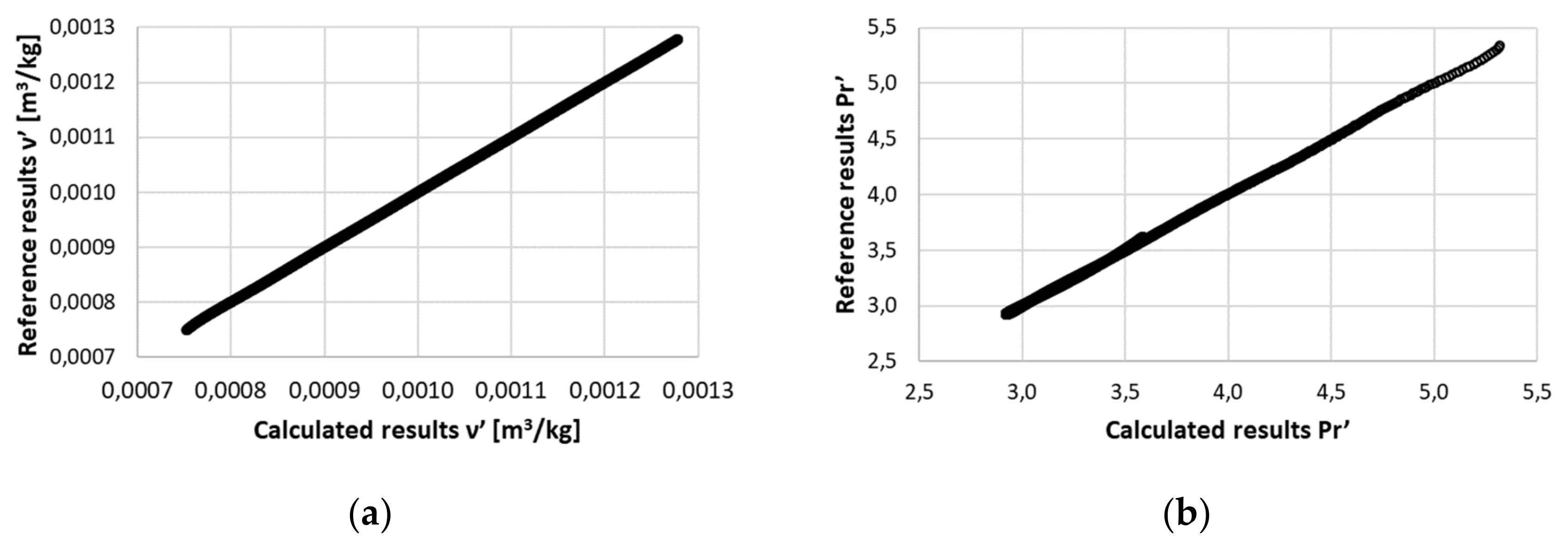
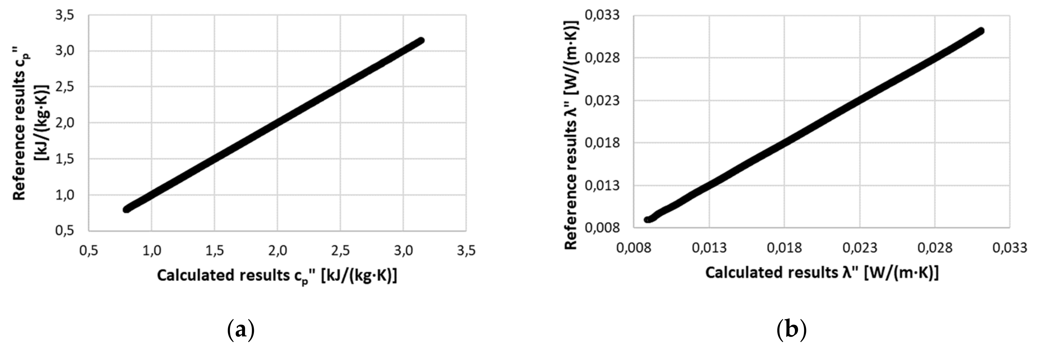
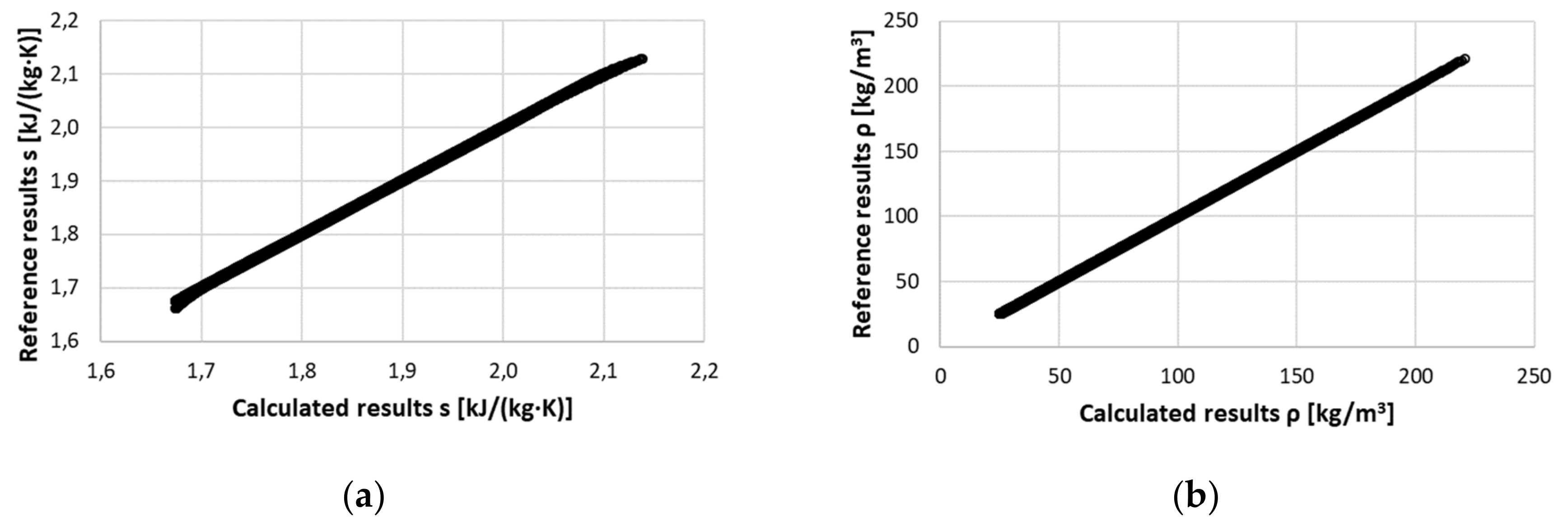
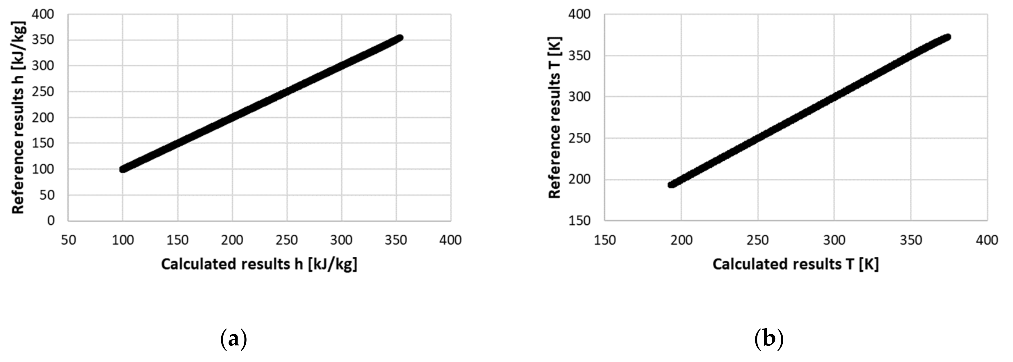
The maximum average relative deviation was 0.164% (Equation (9)). The average relative deviation only exceeded 0.1% in three equations (Equations (9), (16) and (20)). The maximum relative deviation did not exceed 1% in any of the 26 equations. The largest maximum relative deviation occurred in the equation describing the Prandtl number of saturated liquid and was equal to 0.974%. Comparisons of the reference and calculated results for the equations with the largest deviations are given in Figure 2, Figure 3, Figure 4 and Figure 5.
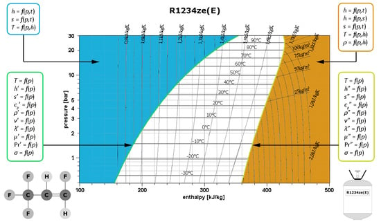
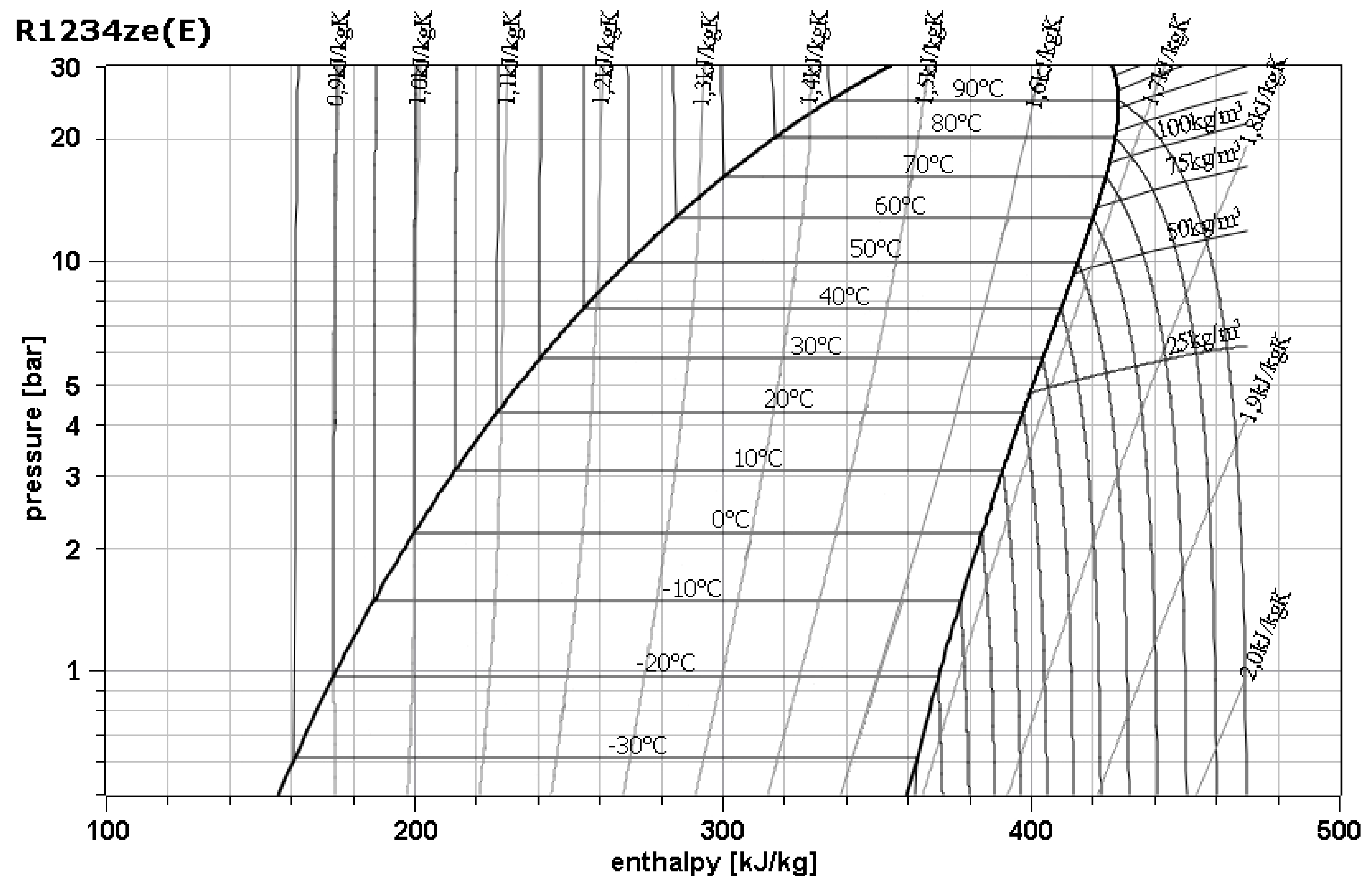
A pressure–enthalpy diagram developed using the equations that describe the thermodynamic properties of the refrigerant is given in Figure 6.
5. Discussion
Traditional methods for determining refrigerant parameters, based on state equations, require complex differential equations to be solved. Therefore, it is important to find new ways to determine the properties of refrigerants characterized by simplicity and speed of operation. The Levenberg–Marquardt non-linear estimation method was used to describe the parameters of the R1234ze(E) refrigerant. Grade 3–9 polynomials were developed to describe each property. The optimal degree of a polynomial depends on the statistical evaluation of the equations obtained. The quality of the created equations was evaluated by the standard criteria used for statistical results evaluation: the correlation coefficient, determination coefficient, and relative and absolute deviations. Statistical verification was carried out on much more data than the amount used to create equations. The results of the analysis shown in Table 11, Table 12 and Table 13 show that the results obtained for the R1234ze(E) refrigerant properties are very similar to the data obtained from the CoolProp program. Relative deviations do not exceed 1% for any relationship. Figure 2, Figure 3, Figure 4 and Figure 5 show the relationships between the calculated and given values of the properties of R1234ze(E) for equations with the largest deviations. The charts clearly show that the results are very similar to the CoolProp data.
A certain limitation on the use of equations is the scope of their validity given in Table 2. However, this range is sufficient for the simulation of refrigeration systems or the analysis of refrigeration equipment operations. The method used can be employed to develop equations for other refrigerants.
6. Conclusions
Thermodynamic analyses of refrigeration cycles require knowledge of refrigerant properties. Due to the limitations on the use of HFC refrigerants, HFO refrigerants are increasingly being used. The equations formulated in this paper make it possible to determine the properties of the R1234ze(E) refrigerant in the saturation, subcooled liquid, and superheated vapour states. The equations are given in an accessible form and the determined coefficients have low deviation values. For saturated liquid, the maximum relative deviation was found to slightly exceed 0.97% (equation describing the Prandtl number). For saturated vapour, the maximum relative deviation was found to apply to the equation describing the heat transfer coefficient (0.90%). For superheated vapour, the maximum relative deviation was found to refer to the equation describing density (0.87%). Finally, for subcooled liquid, the maximum relative deviation concerned the temperature (0.41%). The average relative deviations were considerably smaller, not exceeding 0.17% in any of the 26 equations. The main advantages of the equations created are the speed of calculation (no need for numerical calculations), the low deviation values, the scope of application (saturated liquid, saturated steam, superheated steam, supercooled liquid), and the fact that only one variable of the saturation state is required.
Author Contributions
Conceptualization, P.Ż. and M.B.; methodology, P.Ż. and M.B.; software, R.Ł.; validation, Z.K., R.Ł. and B.P.; formal analysis, P.Ż. and R.Ł.; investigation, M.B. and P.Ż.; resources, M.B.; data curation, R.Ł. and Z.K.; writing—original draft preparation, B.P.; writing—review and editing, M.B.; visualization, Z.K. and B.P.; supervision, P.Ż.; project administration, P.Ż.; funding acquisition, M.B. All authors have read and agreed to the published version of the manuscript.
Funding
This research received no external funding.
Conflicts of Interest
The authors declare no conflict of interest.
References
- Regulation (EU) No 517/2014 of the European Parliament and of the Council of 16 April 2014 on Fluorinated Greenhouse Gases and Repealing Regulation (EC) No 842/2006. OJ L 150, 20.5.2014; pp. 195–230. Available online: http://data.europa.eu/eli/reg/2014/517/oj (accessed on 2 December 2019).
- European Environment Agency. Fluorinated Greenhouse Gases 2018. Data Reported by Companies on the Production, Import, Export and Destruction of Fluorinated Greenhouse Gases in the European Union, 2007–2017; EEA Report No 21/2018; Publications Office of the European Union: Luxembourg, 2018. [Google Scholar]
- Lemmon, E.W.; Huber, M.L.; McLinden, M.O. REFPROP, NIST Standard Reference Database 23, v.9.1; National Institute of Standards: Gaithersburg, MD, USA, 2014. [Google Scholar]
- Myhre, G.; Shindell, D.; Bréon, F.-M.; Collins, W.; Fuglestvedt, J.; Huang, J.; Koch, D.; Lamarque, J.-F.; Lee, D.; Mendoza, B.; et al. Anthropogenic and Natural Radiative Forcing. In Climate Change 2013: The Physical Science Basis. Contribution of Working Group I to the Fifth Assessment Report of the Intergovernmental Panel on Climate Change; Stocker, T.F.D., Qin, G.-K., Plattner, M., Tignor, S.K., Allen, J., Boschung, A., Nauels, Y., Xia, V.B., Midgley, P.M., Eds.; Cambridge University Press: Cambridge, UK; New York, NY, USA, 2013. [Google Scholar]
- Sethi, A.; Becerra, E.V.; Motta, S.Y. Low GWP R134a replacements for small refrigeration (plug-in) applications. Int. J. Refrig. 2016, 66, 64–72. [Google Scholar] [CrossRef]
- Moles, F.; Navarro-Esbri, J.; Peris, B.; Mota-Babiloni, A.; Mateu-Royo, C. R1234yf and R1234ze as alternatives to R134a in Organic Rankine Cycles for low temperature heat sources. Energy Procedia 2017, 142, 1192–1198. [Google Scholar] [CrossRef]
- Devecioglu, A.G.; Oruc, V. Improvement on the energy performance of a refrigeration system adapting a plate-type heat exchanger and low-GWP refrigerants as alternatives to R134a. Energy 2018, 155, 105–116. [Google Scholar] [CrossRef]
- Devecioglu, A.G.; Oruc, V. A comparative energetic analysis for some low-GWP refrigerants as R134a replacements in various vapor compression refrigeration systems. Isı Bilimi Ve Tek. Tek. I Derg. J. Therm. Sci. Technol. 2018, 38, 51–61. [Google Scholar]
- Ben Jemaa, R.; Mansouri, R.; Boukholda, I.; Bellagi, A. Energy and exergy investigation of R1234ze as R134a replacement in vapor compression chillers. Int. J. Hydrog. Energy 2017, 42, 12877–12887. [Google Scholar] [CrossRef]
- Jankovic, Z.; Sieres Atienza, J.; Martinez Suarez, J.A. Thermodynamic and heat transfer analyses for R1234yf and R1234ze(E) as drop-in replacements for R134a in a small power refrigerating system. Appl. Therm. Eng. 2015, 80, 42–54. [Google Scholar] [CrossRef]
- Mota-Babiloni, A.; Navarro-Esbri, J.; Barragan-Cervera, A.; Moles, F.; Peris, B. Drop-in analysis of an internal heat exchanger in a vapour compression system using R1234ze(E) and R450A as alternatives for R134a. Energy 2015, 90, 1636–1644. [Google Scholar] [CrossRef] [Green Version]
- Sanchez, D.; Cabello, R.; Llopis, R.; Arauzo, I.; Catalan-Gil, J.; Torrella, E. Energy performance evaluation of R1234yf, R1234ze(E), R600a, R290 and R152a as low-GWP R134a alternatives. Int. J. Refrig. 2017, 74, 269–282. [Google Scholar] [CrossRef]
- Meng, Z.; Zhang, H.; Qiu, J.; Lei, M. Theoretical analysis of R1234ze(E), R152a, and R1234ze(E)/R152a mixtures as replacements of R134a in vapor compression system. Adv. Mech. Eng. 2016, 8, 1–10. [Google Scholar] [CrossRef] [Green Version]
- Bansal, P.; Shen, B. Analysis of environmentally friendly refrigerant options for window air conditioners. Sci. Technol. Built Environ. 2015, 21, 483–490. [Google Scholar] [CrossRef]
- Mota-Babiloni, A.; Navarro-Esbri, J.; Moles, F.; Barragan-Cervera, A.; Peris, B.; Verdu, G. A review of refrigerant R1234ze(E) recent investigations. Appl. Therm. Eng. 2016, 95, 211–222. [Google Scholar] [CrossRef]
- Lemmon, E.W.; Bell, I.H.; Huber, M.L.; McLinden, M.O. NIST Standard Reference Database 23: Reference Fluid Thermodynamic and Transport Properties-REFPROP, Version 10.0; Standard Reference Data Program; National Institute of Standards and Technology: Gaithersburg, MD, USA, 2018. [Google Scholar]
- Bell, I.H.; Wronski, J.; Quoilin, S.; Lemort, V. Pure and Pseudo-pure Fluid Thermophysical Property Evaluation and the Open-Source Thermophysical Property Library CoolProp. Ind. Eng. Chem. Res. 2014, 53, 2498–2508. [Google Scholar] [CrossRef] [PubMed] [Green Version]
- Butrymowicz, D.; Baj, P.; Śmierciew, K. Technika Chłodnicza; Wydawnictwo Naukowe PWN: Warszawa, Poland, 2014. [Google Scholar]
- Bobbo, S.; Di Nicola, G.; Zilio, C.; Brown, J.S.; Fedele, L. Low GWP halocarbon refrigerants: A review of thermophysical properties. Int. J. Refrig. 2018, 90, 181–201. [Google Scholar] [CrossRef]
- De Monte, F. Calculation of thermodynamic properties of R407C and R410A by the Martin-Hou equation of state—Part I: Theoretical development. Int. J. Refrig. 2002, 25, 306–313. [Google Scholar] [CrossRef]
- De Monte, F. Calculation of thermodynamic properties of R407C and R410A by the Martin-Hou equation of state—Part II: Technical interpretation. Int. J. Refrig. 2002, 25, 314–329. [Google Scholar] [CrossRef]
- Feroiu, V.; Geana, D. Volumetric and thermodynamic properties for pure refrigerants and refrigerant mixtures from cubic equations of state. Fluid Phase Equilibria 2003, 207, 283–300. [Google Scholar] [CrossRef]
- Feroiu, V.; Geana, D. Properties of pure refrigerants and refrigerant mixtures from cubic equations of state. Rev. Roum. De Chmie 2011, 56, 517–525. [Google Scholar]
- Ding, G.; Wu, Z.; Liu, J.; Inagaki, T.; Wang, K.; Fukaya, M. An implicit curve-fitting method for fast calculation of thermal properties of pure and mixed refrigerant. Int. J. Refrig. 2005, 28, 921–932. [Google Scholar] [CrossRef]
- Sozen, A.; Arcaklioglu, E.; Menlik, T.; Ozalp, M. Determination of thermodynamic properties of an alternative refrigerant (R407C) using artificial neural network. Expert Syst. Appl. 2009, 36, 4346–4356. [Google Scholar] [CrossRef]
- Sozen, A.; Arcaklioglu, E.; Menlik, T. Derivation of empirical equations for thermodynamic properties of a ozone safe refrigerant (R404a) using artificial neural network. Expert Syst. Appl. 2010, 37, 1158–1168. [Google Scholar] [CrossRef]
- Sencan, A.; Kose, I.I.; Selbas, R. Comparative analysis of neural network and neuro-fuzzy system for thermodynamic properties of refrigerants. Appl. Artif. Intell. 2012, 26, 662–672. [Google Scholar] [CrossRef]
- Yilmaz, H.; Sencan, A.; Selbas, R. An estimation of thermodynamic properties of hydrocarbon refrigerants. Int. J. Green Energy 2014, 11, 500–526. [Google Scholar] [CrossRef]
- Mora, R.J.E.; Perez, T.C.; Gonzalez, N.F.F.; Ocampo, D.J.D.D. Thermodynamic properties of refrigerants using artificial neural networks. Int. J. Refrig. 2014, 46, 9–16. [Google Scholar] [CrossRef]
- Kucuksille, E.U.; Selbas, R.; Sencan, A. Data mining techniques for thermophysical properties of refrigerants. Energy Convers. Manag. 2009, 50, 399–412. [Google Scholar] [CrossRef]
- Kucuksille, E.U.; Selbas, R.; Sencan, A. Prediction of thermodynamic properties of refrigerants using data mining. Energy Convers. Manag. 2011, 52, 836–848. [Google Scholar] [CrossRef]
- Sieres, J.; Varas, F.; Martinez-Suarez, J.A. A hybrid formulation for fast explicit calculation of thermodynamic properties of refrigerants. Int. J. Refrig. 2012, 35, 1021–1034. [Google Scholar] [CrossRef]
- StatSoft. STATISTICA (Data Analysis Software System), version 12. 2014. Available online: www.statsoft.pl (accessed on 1 October 2019).
- Życzkowski, P. Korelacje obliczeniowe parametrów termodynamicznych i termokinetycznych czynnika chłodniczego R1234yf. Cz. 1, Ciecz nasycona i para nasycona sucha. Chłodnictwo 2016, 3, 18–22. [Google Scholar] [CrossRef]
- Życzkowski, P. Korelacje obliczeniowe parametrów termodynamicznych i termokinetycznych czynnika chłodniczego R1234yf. Cz. 2, Obszar pary przegrzanej i cieczy przechłodzonej. Chłodnictwo 2016, 4, 22–25. [Google Scholar] [CrossRef]
- Nowak, B.; Życzkowski;Łuczak, R. Functional dependence of thermodynamic and thermokinetic parameters of refrigerants used in mine air refrigerators. Part 1, Refrigerant R407C. Arch. Min. Sci. 2017, 62, 55–72. [Google Scholar] [CrossRef] [Green Version]
- Nowak, B.; Życzkowski;Łuczak, R. Functional dependencies of thermodynamic and thermokinetic parameters of refrigerants used in mine air refrigerators. Pt. 2, Refrigerant R404A. Arch. Min. Sci. 2018, 63, 27–41. [Google Scholar] [CrossRef]
- Pires, R.; Mili, L.; Chagas, G. Robust complex-valued Levenberg-Marquardt algorithm as applied to power flow analysis. Electr. Power Energy Syst. 2019, 113, 383–392. [Google Scholar] [CrossRef]
- Cui, M.; Yang, K.; Xu, X.L.; Wang, S.D.; Gao, X.W. A modified Levenberg–Marquardt algorithm for simultaneous estimation of multi-parameters of boundary heat flux by solving transient nonlinear inverse heat conduction problems. Int. J. Heat Mass Transf. 2016, 97, 908–916. [Google Scholar] [CrossRef]
- Yang, K.; Jiang, G.H.; Peng, H.F.; Gao, X.W. A new modified Levenberg-Marquardt algorithm for identifying the temperature-dependent conductivity of solids based on the radial integration boundary element method. Int. J. Heat Mass Transf. 2019, 144, 118615. [Google Scholar] [CrossRef]
- Tossa, A.K.; Soro, Y.M.; Azoumah, Y.; Yamegueu, D. A new approach to estimate the performance and energy productivity of photovoltaic modules in real operating conditions. Sol. Energy 2014, 110, 543–560. [Google Scholar] [CrossRef]
- Blaifi, S.; Moulahoum, S.; Taghezouit, B.; Saim, A. An enhanced dynamic modeling of PV module using Levenberg-Marquardt algorithm. Renew. Energy 2019, 135, 745–760. [Google Scholar] [CrossRef]
- Koppel, T.; Vassiljev, A. Calibration of a model of an operational water distribution system containing pipes of different age. Adv. Eng. Softw. 2009, 40, 659–664. [Google Scholar] [CrossRef]
Figure 1.
Pressure–enthalpy diagram of a theoretical refrigeration cycle.

Figure 2.
Comparison of the reference results and calculated results for saturated liquid: (a) Specific volume; (b) Prandtl number.
Figure 2.
Comparison of the reference results and calculated results for saturated liquid: (a) Specific volume; (b) Prandtl number.

Figure 3.
Comparison of the reference results and calculated results for saturated vapour: (a) Specific heat; (b) Heat transfer coefficient.
Figure 3.
Comparison of the reference results and calculated results for saturated vapour: (a) Specific heat; (b) Heat transfer coefficient.

Figure 4.
Comparison of the reference results and calculated results for superheated vapour: (a) Specific entropy; (b) Density.
Figure 4.
Comparison of the reference results and calculated results for superheated vapour: (a) Specific entropy; (b) Density.

Figure 5.
Comparison of the reference results and calculated results for subcooled liquid: (a) Specific entropy; (b) Temperature.
Figure 5.
Comparison of the reference results and calculated results for subcooled liquid: (a) Specific entropy; (b) Temperature.

Figure 6.
Diagram of the thermodynamic properties of the R1234ze(E) refrigerant.


| Property | Value |
|---|---|
| Group | HFO |
| Chemical formula | trans-CF3CH = CHF |
| Molar mass, kg/kmol | 114 |
| Critical temperature, °C | 109.36 |
| Critical pressure, bar | 36.4 |
| Critical density, kg/m3 | 489.2 |
| Normal boiling point, °C | −19.3 |
| Triple point, °C | −104.53 |
| ODP (ozone depletion potential) | 0 |
| GWP20 (global warming potential) 20 years | 4 |
| GWP100 (global warming potential) 100 years | 1 |
| Atmospheric lifetime of individual components, days | 16.4 |
Table 2.
The scope of equations describing the properties of the R1234ze(E) refrigerant and the amount of data used for analysis.
Table 2.
The scope of equations describing the properties of the R1234ze(E) refrigerant and the amount of data used for analysis.
| State | Scope | Amount of Data |
|---|---|---|
| Saturated liquid | p: 0.5–30.0 bar | 591 |
| Saturated vapour | p: 0.5–30.0 bar | 591 |
| Superheated vapour | p: 0.5–30.0 bar; t: t″ − 120 °C | 18,186 1 |
| Subcooled liquid | p: 0.5–30.0 bar; t: −80 °C−t′ | 41,901 |
1 for ρ from 25 kg/m3 and up to 470 kJ/kg; 9608 pieces of data.
Table 3.
Coefficients of polynomials describing the temperature, specific enthalpy, specific entropy, and specific heat of the R1234ze(E) refrigerant in the saturated liquid state.
Table 3.
Coefficients of polynomials describing the temperature, specific enthalpy, specific entropy, and specific heat of the R1234ze(E) refrigerant in the saturated liquid state.
| Coef | Equation | |||
|---|---|---|---|---|
| T = f(p) (1) | h′ = f(p) (2) | s′ = f(p) (3) | cp′ = f(p) (4) | |
| a0 | 2.53879921713140 × 10² | 1.74968285360988 × 10² | 9.05279244602078 × 10⁻¹ | 1.24083270657197 |
| a1 | 2.28770347319237 × 101 | 2.93484680604720 × 101 | 1.15356542959209 × 10⁻¹ | 4.51902938229883 × 10⁻² |
| a2 | 2.45670755735841 | 3.00047504671966 | 7.24618471191152 × 10⁻³ | −5.63723496516354 × 10⁻³ |
| a3 | 3.14117394078267 × 10⁻¹ | 1.19253718641735 | 2.73012551482764 × 10⁻³ | 6.42959196900272 × 10⁻⁴ |
| a4 | −6.76941445013617 × 10⁻² | 6.99952705225739 × 10⁻¹ | 1.71764538194706 × 10⁻³ | −3.54112766926212 × 10⁻⁵ |
| a5 | 4.07277016474858 × 10⁻² | −1.51604024263818 | −3.86378154015459 × 10⁻³ | 5.37559165828602 × 10⁻⁷ |
| a6 | −5.95404205600932 × 10⁻³ | 9.67067796211943 × 10⁻¹ | 2.45968598111626 × 10⁻³ | 3.84386880084408 × 10⁻⁸ |
| a7 | - | −2.62092375289440 × 10⁻¹ | −6.67334247116959 × 10⁻⁴ | −1.88423766967265 × 10⁻⁹ |
| a8 | - | 2.66563442687942 × 10⁻² | 6.78181882644024 × 10⁻⁵ | 2.54741811878324 × 10⁻¹¹ |
Table 4.
Coefficients of polynomials describing the density, specific volume, and heat transfer coefficient of the R1234ze(E) refrigerant in the saturated liquid state.
Table 4.
Coefficients of polynomials describing the density, specific volume, and heat transfer coefficient of the R1234ze(E) refrigerant in the saturated liquid state.
| Coef | Equation | ||
|---|---|---|---|
| ρ′ = f(p) (5) | ν′ = f(p) (6) | λ′ = f(p) (7) | |
| a0 | 1.29396343579499 × 10³ | 7.29710663744474 × 10⁻⁴ | 9.03143423982640 × 10⁻² |
| a1 | −6.20669713392757 × 101 | 5.01608980784443 × 10⁻⁵ | −8.80066599536261 × 10⁻³ |
| a2 | −2.53752547194416 | −9.30886654653688 × 10⁻⁶ | −9.99542811098308 × 10⁻⁴ |
| a3 | −9.31562506661149 | 1.37045258345160 × 10⁻⁶ | 2.92095921761060 × 10⁻⁴ |
| a4 | −7.20333951838005 | −1.23148305617849 × 10⁻⁷ | 3.50549588319595 × 10⁻⁴ |
| a5 | 1.64294878085487 × 101 | 6.76679411090488 × 10⁻⁹ | −7.30082138730070 × 10⁻⁴ |
| a6 | −1.04093686983023 × 101 | −2.20602504790423 × 10⁻¹⁰ | 4.40360054711903 × 10⁻⁴ |
| a7 | 2.81591566729637 | 3.91341788788786 × 10⁻¹² | −1.14689158182047 × 10⁻⁴ |
| a8 | −2.86461830242391 × 10⁻¹ | −2.90062006624196 × 10⁻¹⁴ | 1.10956525980123 × 10⁻⁵ |
Table 5.
Coefficients of polynomials describing the dynamic viscosity coefficient, Prandtl number, and surface tension of the R1234ze(E) refrigerant in the saturated liquid state.
Table 5.
Coefficients of polynomials describing the dynamic viscosity coefficient, Prandtl number, and surface tension of the R1234ze(E) refrigerant in the saturated liquid state.
| Coef | Equation | ||
|---|---|---|---|
| µ′ = f(p) (8) | Pr′ = f(p) (9) | σ = f(p) (10) | |
| a0 | 3.30126989957222 × 10⁻⁴ | 4.67836170077957 | 1.59343062468816 × 10⁻² |
| a1 | −1.03228385472871 × 10⁻⁴ | −8.07941153808255 × 10⁻¹ | −4.27582523407763 × 10⁻³ |
| a2 | 1.09405636740428 × 10⁻⁵ | 1.78574619681131 × 10⁻¹ | 1.08824350295615 × 10⁻⁵ |
| a3 | −1.54688847220722 × 10⁻⁶ | −4.54256602128744 × 10⁻¹ | −2.88012392508621 × 10⁻⁵ |
| a4 | −2.44961988256085 × 10⁻⁷ | 1.75299143854024 × 10⁻¹ | 1.02007105181399 × 10⁻⁵ |
| a5 | 9.19517023370312 × 10⁻⁷ | 5.54715409594885 × 10⁻¹ | −3.46263550356762 × 10⁻⁵ |
| a6 | −6.03952237218337 × 10⁻⁷ | −6.97630428910946 × 10⁻¹ | 2.31347786949313 × 10⁻⁵ |
| a7 | 1.66816987767627 × 10⁻⁷ | 3.38689978995674 × 10⁻¹ | −6.30855999198157 × 10⁻⁶ |
| a8 | −1.71375788331681 × 10⁻⁸ | −7.62417081213265 × 10⁻² | 6.68652044821767 × 10⁻⁷ |
| a9 | - | 6.62560394142489 × 10⁻³ | - |
Table 6.
Coefficients of polynomials describing the specific enthalpy, specific entropy, specific heat, and density of the R1234ze(E) refrigerant in the saturated vapour state.
Table 6.
Coefficients of polynomials describing the specific enthalpy, specific entropy, specific heat, and density of the R1234ze(E) refrigerant in the saturated vapour state.
| Coef | Equation | |||
|---|---|---|---|---|
| h″ = f(p) (11) | s″ = f(p) (12) | cp″ = f(p) (13) | ρ″ = f(p) (14) | |
| a0 | 3.70657366815286 × 10² | 1.67622654205859 | 7.63398360227738 × 10⁻¹ | 2.27768588078390 × 10⁻¹ |
| a1 | 1.62926056610703 × 101 | −5.81493952118715 × 10⁻³ | 7.32627000545461 × 10⁻² | 5.54068367754339 |
| a2 | 2.46905883267318 | 6.61688503765656 × 10⁻³ | −1.06783110270413 × 10⁻² | −1.70610755621257 × 10⁻¹ |
| a3 | −1.13621954845305 | −2.94796323909036 × 10⁻³ | 1.22686997407115 × 10⁻³ | 3.58297189467255 × 10⁻² |
| a4 | −1.08070437166134 | −2.75644193419488 × 10⁻³ | −7.15472829720056 × 10⁻⁵ | −3.97722125575951 × 10⁻³ |
| a5 | 2.49195790709675 | 6.33081705594435 × 10⁻³ | 1.61584178260620 × 10⁻⁶ | 2.97586911550852 × 10⁻⁴ |
| a6 | −1.57431720780436 | −3.99095180784525 × 10⁻³ | 3.78799626428319 × 10⁻⁸ | −1.42888359942333 × 10⁻⁵ |
| a7 | 4.25121219497403 × 10⁻¹ | 1.07579556459832 × 10⁻³ | −2.62846106511664 × 10⁻⁹ | 4.26062135708768 × 10⁻⁷ |
| a8 | −4.32428413533420 × 10⁻² | −1.09130621835064 × 10⁻⁴ | 3.84463040954545 × 10⁻¹¹ | −7.16416594446346 × 10⁻⁹ |
| a9 | - | - | - | 5.23362423501008 × 10⁻¹¹ |
Table 7.
Coefficients of polynomials describing the specific volume, heat transfer coefficient, dynamic viscosity coefficient, and Prandtl number of the R1234ze(E) refrigerant in the saturated vapour state.
Table 7.
Coefficients of polynomials describing the specific volume, heat transfer coefficient, dynamic viscosity coefficient, and Prandtl number of the R1234ze(E) refrigerant in the saturated vapour state.
| Coef | Equation | |||
|---|---|---|---|---|
| ν″ = f(p) (15) | λ″ = f(p) (16) | µ″ = f(p) (17) | Pr″ = f(p) (18) | |
| a0 | 1.77433953172014 × 10⁻¹ | 1.00685420897056 × 10⁻² | 1.05062529128478 × 10⁻⁵ | 8.74440749215016 × 10⁻¹ |
| a1 | −1.66936428639188 × 10⁻¹ | 2.01521099378549 × 10⁻³ | 9.52821100098587 × 10⁻⁷ | −2.39936282800067 × 10⁻² |
| a2 | 7.75579038246079 × 10⁻² | 4.91117080105326 × 10⁻⁴ | −3.00951147568936 × 10⁻⁷ | 1.25205016486864 × 10⁻² |
| a3 | −2.41489018240415 × 10⁻² | −1.75824023764422 × 10⁻³ | 5.32152051905147 × 10⁻⁷ | −2.27389415072141 × 10⁻³ |
| a4 | 5.61391538794325 × 10⁻³ | 7.60350748872995 × 10⁻⁴ | 4.70502421614829 × 10⁻⁷ | 2.36745600186706 × 10⁻⁴ |
| a5 | −9.65998396886106 × 10⁻⁴ | 2.19935489007404 × 10⁻³ | −1.09002347169414 × 10⁻⁶ | −1.45822262459754 × 10⁻⁵ |
| a6 | 9.87363959178734 × 10⁻⁵ | −2.83720578521593 × 10⁻³ | 6.84901655972941 × 10⁻⁷ | 5.30654276070867 × 10⁻⁷ |
| a7 | −7.48240927743627 × 10⁻⁷ | 1.40136740639282 × 10⁻³ | −1.84631268281049 × 10⁻⁷ | −1.05453244596624 × 10⁻⁸ |
| a8 | −7.07631682979349 × 10⁻⁷ | −3.20515361896471 × 10⁻⁴ | 1.86385265681204 × 10⁻⁸ | 8.89411840080677 × 10⁻¹¹ |
| a9 | - | 2.83753380724076 × 10⁻⁵ | - | - |
Table 8.
Coefficients of polynomials describing the properties of the R1234ze(E) refrigerant in the superheated vapour state (h = f(p,t), h = f(p,s), s = f(p,t)).
Table 8.
Coefficients of polynomials describing the properties of the R1234ze(E) refrigerant in the superheated vapour state (h = f(p,t), h = f(p,s), s = f(p,t)).
| Coef | Equation | ||
|---|---|---|---|
| h = f(p,t) (19) | h = f(p,s) (20) | s = f(p,t) (21) | |
| a1 | −1.22538219116946 × 101 | 9.70737789929653 | 1.02201325065485 × 10³ |
| a2 | −1.19684176263820 × 10⁻¹ | 2.61874436156932 × 10⁻¹ | 2.11930425863317 |
| a3 | 2.56418987553419 × 10⁻² | 7.03198731354432 × 10⁻² | −2.25093762714879 × 10⁻¹ |
| a4 | 1.12370072751876 × 10⁻¹ | 2.04713651916276 × 10⁻¹ | −4.13156661967710 × 10⁻¹ |
| a5 | −7.84589730210466 × 10⁻² | - | −2.66667859197166 × 10⁻¹ |
| b1 | 1.07613121977651 × 101 | 2.14480351606632 × 10² | −7.38442317160207 |
| b2 | 1.27909162098184 × 10⁻¹ | 8.78348541751969 | −1.54691107365295 × 10⁻² |
| b3 | −2.17557771059542 × 10⁻² | 2.33196204712552 | 1.61160247230101 × 10⁻³ |
| b4 | −1.33475632720526 × 10⁻² | 6.31343053191083 | 4.11509116217012 × 10⁻³ |
| b5 | 1.30152145421200 × 10⁻² | - | 2.68867618687700 × 10⁻³ |
| c1 | 9.20939997738017 × 10² | 1.30915602277249 × 10² | 1.00415786839940 × 10⁴ |
| c2 | −1.70804798986579 × 101 | 6.23649470729840 | −1.12883262503797 × 10² |
| c3 | −9.36024775369566 | 1.07200578512649 | −2.83482394816380 × 101 |
| c4 | 6.34415745181292 × 10⁻¹ | −2.26086399298466 | −9.09256164033981 × 10⁻¹ |
| c5 | −1.25745577415437 | - | −1.13294272169830 |
Table 9.
Coefficients of polynomials describing the properties of the R1234ze(E) refrigerant in the superheated vapour state (T = f(p,h), ρ = f(p,h)).
Table 9.
Coefficients of polynomials describing the properties of the R1234ze(E) refrigerant in the superheated vapour state (T = f(p,h), ρ = f(p,h)).
| Coef | Equation | |
|---|---|---|
| T = f(p,h) (22) | ρ = f(p,h) (23) | |
| a1 | 1.80123820111647 × 101 | 2.81203869542640 × 101 |
| a2 | 8.24003323530265 × 10⁻² | 1.15184541343782 × 10⁻¹ |
| a3 | 2.51686613531001 × 10⁻² | 2.45938820598331 |
| a4 | - | 8.43110685237400 × 10⁻¹ |
| a5 | - | −2.05663545341847 × 10⁻³ |
| a6 | - | 1.15342507562934 |
| b1 | −9.57478728374795 | −2.27670387576552 × 101 |
| b2 | −4.92373151059871 × 10⁻² | 3.83041059824037 |
| b3 | 1.88344691904411 × 10⁻² | −4.86420752353526 |
| b4 | - | −1.09064973382657 × 101 |
| b5 | - | −1.20058186844573 × 10⁻¹ |
| b6 | - | −4.74405743126640 |
| c1 | −6.16759701982095 × 10³ | 2.65873399640243 × 10² |
| c2 | −8.19380014241848 × 101 | −2.22556557307299 × 101 |
| c3 | −1.11076735383728 × 101 | 2.57855441990927 × 101 |
| c4 | - | 6.47202322127270 × 101 |
| c5 | - | −1.99964641247140 |
| c6 | - | 2.66402045824145 × 101 |
Table 10.
Coefficients of polynomials describing the properties of the R1234ze(E) refrigerant in the subcooled liquid state (h = f(p,t), s = f(p,t), T = f(p,h)).
Table 10.
Coefficients of polynomials describing the properties of the R1234ze(E) refrigerant in the subcooled liquid state (h = f(p,t), s = f(p,t), T = f(p,h)).
| Coef | Equation | ||
|---|---|---|---|
| h = f(p,t) (24) | s = f(p,t) (25) | T = f(p,h) (26) | |
| a1 | −1.24632495027227 × 10² | 1.53492509731654 | −2.54401494933800 |
| a2 | −8.93767310439441 × 10⁻² | 1.14188030931082 × 10⁻² | 1.41981737305051 × 10⁻² |
| a3 | −5.13970645120413 × 10⁻³ | −2.27977637362198 × 10⁻³ | 4.17004268014005 × 10⁻³ |
| a4 | −7.81419045658094 × 10⁻⁴ | −9.09151613042750 × 10⁻⁴ | −4.57959473157251 × 10⁻³ |
| a5 | 4.22545925349730 × 10⁻⁴ | −4.02681309084223 × 10⁻⁴ | - |
| a6 | 3.59229939083742 × 10⁻⁴ | - | - |
| b1 | −8.14460833381591 × 10³ | −8.64303643796513 | 8.02627024648105 |
| b2 | −6.05289428492502 | −6.37870935254633 × 10⁻² | −4.09757320861048 × 10⁻² |
| b3 | −3.94885910243123 × 10⁻¹ | 1.30109052596914 × 10⁻² | −1.18576883918572 × 10⁻² |
| b4 | −7.25230146369704 × 10⁻² | 5.37778256355485 × 10⁻³ | 1.08815116545496 × 10⁻³ |
| b5 | 2.69851262120827 × 10⁻² | 4.62322186390055 × 10⁻³ | - |
| b6 | 1.40090835277157 × 10⁻² | - | - |
| c1 | 5.51597947695862 × 10⁵ | 1.05287623121195 × 10³ | −7.10087317464252 × 10³ |
| c2 | −3.62158965210490 × 10² | −2.75983526288628 × 101 | 8.50746165042646 × 101 |
| c3 | −5.21112983842346 × 101 | −1.25845749595145 × 101 | −2.84134460440402 |
| c4 | −1.64400591142357 × 101 | −3.66028024779350 | −6.47159328560425 × 10⁻¹ |
| c5 | −1.44044662909068 × 101 | −3.23703650445058 × 10⁻¹ | - |
| c6 | −4.26763585954523 | - | - |
Table 11.
Correlation and determination coefficients of the equations used to calculate the properties of the R1234ze(E) refrigerant.
Table 11.
Correlation and determination coefficients of the equations used to calculate the properties of the R1234ze(E) refrigerant.
| Equation | Region | Correlation Coefficient R | Determination Coefficient R2 | |
|---|---|---|---|---|
| T = f(p) | (1) | Saturated liquid, saturated vapour | 0,9999999955 | 0,9999999910 |
| h′ = f(p) | (2) | Saturated liquid | 0.9999999077 | 0.9999998155 |
| s′ = f(p) | (3) | Saturated liquid | 0.9999999361 | 0.9999998722 |
| cp′ = f(p) | (4) | Saturated liquid | 0.9999992806 | 0.9999985612 |
| ρ′ = f(p) | (5) | Saturated liquid | 0.9999986910 | 0.9999973820 |
| ν′ = f(p) | (6) | Saturated liquid | 0.9999976596 | 0.9999953191 |
| λ′ = f(p) | (7) | Saturated liquid | 0.9999991886 | 0.9999983771 |
| µ′ = f(p) | (8) | Saturated liquid | 0.9999999800 | 0.9999999600 |
| Pr′ = f(p) | (9) | Saturated liquid | 0.9998688664 | 0.9997377499 |
| σ = f(p) | (10) | Saturated liquid, saturated vapour | 0.9999999943 | 0.9999999886 |
| h″ = f(p) | (11) | Saturated vapour | 0.9999976439 | 0.9999952879 |
| s″ = f(p) | (12) | Saturated vapour | 0.9998810558 | 0.9997621258 |
| cp″ = f(p) | (13) | Saturated vapour | 0.9999988802 | 0.9999977605 |
| ρ″ = f(p) | (14) | Saturated vapour | 0.9999999996 | 0.9999999992 |
| ν″ = f(p) | (15) | Saturated vapour | 0.9999999996 | 0.9999999991 |
| λ″ = f(p) | (16) | Saturated vapour | 0.9999895746 | 0.9999791493 |
| µ″ = f(p) | (17) | Saturated vapour | 0.9999806274 | 0.9999612552 |
| Pr″ = f(p) | (18) | Saturated vapour | 0.9999988314 | 0.9999976628 |
| h = f(p,t) | (19) | Superheated vapour | 0.9999843304 | 0.9999686611 |
| h = f(p,s) | (20) | Superheated vapour | 0.9995097223 | 0.9990196850 |
| s = f(p,t) | (21) | Superheated vapour | 0.9999351748 | 0.9998703538 |
| T = f(p,h) | (22) | Superheated vapour | 0.9999471203 | 0.9998942434 |
| ρ = f(p,h) | (23) | Superheated vapour | 0.9999989879 | 0.9999979758 |
| h = f(p,t) | (24) | Subcooled liquid | 0.9999996924 | 0.9999993847 |
| s = f(p,t) | (25) | Subcooled liquid | 0.9999996140 | 0.9999992279 |
| T = f(p,h) | (26) | Subcooled liquid | 0.9999981133 | 0.9999962267 |
Table 12.
Absolute deviations between the values obtained from CoolProp 5.1.1 and the calculated values for the R1234ze(E) refrigerant.
Table 12.
Absolute deviations between the values obtained from CoolProp 5.1.1 and the calculated values for the R1234ze(E) refrigerant.
| Equation | Region | Absolute Deviation | ||
|---|---|---|---|---|
| T = f(p) | (1) | Saturated liquid, saturated vapour | average, K | 0.002499 |
| maximum, K | 0.015994 | |||
| h′ = f(p) | (2) | Saturated liquid | average, kJ/kg | 0.016781 |
| maximum, kJ/kg | 0.091438 | |||
| s′ = f(p) | (3) | Saturated liquid | average, kJ/(kg·K) | 0.000043 |
| maximum, kJ/(kg·K) | 0.000234 | |||
| cp′ = f(p) | (4) | Saturated liquid | average, kJ/(kg·K) | 0.000344 |
| maximum, kJ/(kg·K) | 0.002936 | |||
| ρ′ = f(p) | (5) | Saturated liquid | average, kg/m3 | 0.180720 |
| maximum, kg/m3 | 0.977343 | |||
| ν′ = f(p) | (6) | Saturated liquid | average, m3/kg | 1.99 × 10⁻⁷ |
| maximum, m3/kg | 3.00 × 10⁻⁶ | |||
| λ′ = f(p) | (7) | Saturated liquid | average, W/(m·K) | 1.01 × 10⁻⁵ |
| maximum, W/(m·K) | 6.89 × 10⁻⁵ | |||
| µ′ = f(p) | (8) | Saturated liquid | average, kg/(m·s) | 1.03 × 10⁻⁸ |
| maximum, kg/(m·s) | 5.70 × 10⁻⁸ | |||
| Pr′ = f(p) | (9) | Saturated liquid | average, - | 0.005346 |
| maximum, - | 0.035289 | |||
| σ = f(p) | (10) | Saturated liquid, saturated vapour | average, N/m | 3.49 × 10⁻⁷ |
| maximum, N/m | 1.70 × 10⁻⁶ | |||
| h″ = f(p) | (11) | Saturated vapour | average, kJ/kg | 0.027309 |
| maximum, kJ/kg | 0.144573 | |||
| s″ = f(p) | (12) | Saturated vapour | average, kJ/(kg·K) | 0.000069 |
| maximum, kJ/(kg·K) | 0.000368 | |||
| cp″ = f(p) | (13) | Saturated vapour | average, kJ/(kg·K) | 0.000643 |
| maximum, kJ/(kg·K) | 0.006157 | |||
| ρ″ = f(p) | (14) | Saturated vapour | average, kg/m3 | 0.001151 |
| maximum, kg/m3 | 0.017800 | |||
| ν″ = f(p) | (15) | Saturated vapour | average, m3/kg | 9.46 × 10⁻⁷ |
| maximum, m3/kg | 4.97 × 10⁻⁶ | |||
| λ″ = f(p) | (16) | Saturated vapour | average, W/(m·K) | 1.99 × 10⁻⁵ |
| maximum, W/(m·K) | 1.18 × 10⁻⁴ | |||
| µ″ = f(p) | (17) | Saturated vapour | average, kg/(m·s) | 1.23 × 10⁻⁸ |
| maximum, kg/(m·s) | 6.80 × 10⁻⁸ | |||
| Pr″ = f(p) | (18) | Saturated vapour | average, - | 0.000263 |
| maximum, - | 0.005100 | |||
| h = f(p,t) | (19) | Superheated vapour | average, kJ/kg | 0.094327 |
| maximum, kJ/kg | 1.561120 | |||
| h = f(p,s) | (20) | Superheated vapour | average, kJ/kg | 0.683322 |
| maximum, kJ/kg | 3.484118 | |||
| s = f(p,t) | (21) | Superheated vapour | average, kJ/(kg·K) | 0.000729 |
| maximum, kJ/(kg·K) | 0.013665 | |||
| T = f(p,h) | (22) | Superheated vapour | average, K | 0.237796 |
| maximum, K | 2.891388 | |||
| ρ = f(p,h) | (23) | Superheated vapour | average, kg/m3 | 0.047104 |
| maximum, kg/m3 | 0.437241 | |||
| h = f(p,t) | (24) | Subcooled liquid | average, kJ/kg | 0.028842 |
| maximum, kJ/kg | 1.109729 | |||
| s = f(p,t) | (25) | Subcooled liquid | average, kJ/(kg·K) | 0.000121 |
| maximum, kJ/(kg·K) | 0.004597 | |||
| T = f(p,h) | (26) | Subcooled liquid | average, K | 0.058954 |
| maximum, K | 1.540900 | |||
Table 13.
Relative deviations between the values obtained from CoolProp 5.1.1 and the calculated values for the R1234ze(E) refrigerant.
Table 13.
Relative deviations between the values obtained from CoolProp 5.1.1 and the calculated values for the R1234ze(E) refrigerant.
| Equation | Region | Absolute Deviation, % | ||
|---|---|---|---|---|
| T = f(p) | (1) | Saturated liquid, saturated vapour | average | 0.000762 |
| maximum | 0.006690 | |||
| h′ = f(p) | (2) | Saturated liquid | average | 0.005986 |
| maximum | 0.048023 | |||
| s′ = f(p) | (3) | Saturated liquid | average | 0.003384 |
| maximum | 0.023007 | |||
| cp′ = f(p) | (4) | Saturated liquid | average | 0.020681 |
| maximum | 0.233195 | |||
| ρ′ = f(p) | (5) | Saturated liquid | average | 0.018672 |
| maximum | 0.124958 | |||
| ν′ = f(p) | (6) | Saturated liquid | average | 0.021500 |
| maximum | 0.400597 | |||
| λ′ = f(p) | (7) | Saturated liquid | average | 0.016861 |
| maximum | 0.133656 | |||
| µ′ = f(p) | (8) | Saturated liquid | average | 0.009928 |
| maximum | 0.085166 | |||
| Pr′ = f(p) | (9) | Saturated liquid | average | 0.164049 |
| maximum | 0.973922 | |||
| σ = f(p) | (10) | Saturated liquid, saturated vapour | average | 0.018004 |
| maximum | 0.297914 | |||
| h″ = f(p) | (11) | Saturated vapour | average | 0.006575 |
| maximum | 0.034191 | |||
| s″ = f(p) | (12) | Saturated vapour | average | 0.004143 |
| maximum | 0.022158 | |||
| cp″ = f(p) | (13) | Saturated vapour | average | 0.050334 |
| maximum | 0.777996 | |||
| ρ″ = f(p) | (14) | Saturated vapour | average | 0.006875 |
| maximum | 0.605068 | |||
| ν″ = f(p) | (15) | Saturated vapour | average | 0.009808 |
| maximum | 0.109992 | |||
| λ″ = f(p) | (16) | Saturated vapour | average | 0.108580 |
| maximum | 0.897582 | |||
| µ″ = f(p) | (17) | Saturated vapour | average | 0.082363 |
| maximum | 0.548505 | |||
| Pr″ = f(p) | (18) | Saturated vapour | average | 0.026480 |
| maximum | 0.585967 | |||
| h = f(p,t) | (19) | Superheated vapour | average | 0.021344 |
| maximum | 0.417555 | |||
| h = f(p,s) | (20) | Superheated vapour | average | 0.155244 |
| maximum | 0.817447 | |||
| s = f(p,t) | (21) | Superheated vapour | average | 0.040509 |
| maximum | 0.822705 | |||
| T = f(p,h) | (22) | Superheated vapour | average | 0.065669 |
| maximum | 0.775753 | |||
| ρ = f(p,h) | (23) | Superheated vapour | average | 0.078893 |
| maximum | 0.867133 | |||
| h = f(p,t) | (24) | Subcooled liquid | average | 0.014884 |
| maximum | 0.312942 | |||
| s = f(p,t) | (25) | Subcooled liquid | average | 0.012436 |
| maximum | 0.312932 | |||
| T = f(p,h) | (26) | Subcooled liquid | average | 0.021539 |
| maximum | 0.413421 | |||
© 2020 by the authors. Licensee MDPI, Basel, Switzerland. This article is an open access article distributed under the terms and conditions of the Creative Commons Attribution (CC BY) license (http://creativecommons.org/licenses/by/4.0/).
Share and Cite
MDPI and ACS Style
Życzkowski, P.; Borowski, M.; Łuczak, R.; Kuczera, Z.; Ptaszyński, B. Functional Equations for Calculating the Properties of Low-GWP R1234ze(E) Refrigerant. Energies 2020, 13, 3052. https://doi.org/10.3390/en13123052
AMA Style
Życzkowski P, Borowski M, Łuczak R, Kuczera Z, Ptaszyński B. Functional Equations for Calculating the Properties of Low-GWP R1234ze(E) Refrigerant. Energies. 2020; 13(12):3052. https://doi.org/10.3390/en13123052
Chicago/Turabian StyleŻyczkowski, Piotr, Marek Borowski, Rafał Łuczak, Zbigniew Kuczera, and Bogusław Ptaszyński. 2020. "Functional Equations for Calculating the Properties of Low-GWP R1234ze(E) Refrigerant" Energies 13, no. 12: 3052. https://doi.org/10.3390/en13123052
Note that from the first issue of 2016, this journal uses article numbers instead of page numbers. See further details here.