A Technique for Frequency Converter-Fed Asynchronous Motor Vibration Monitoring and Fault Classification, Applying Continuous Wavelet Transform and Convolutional Neural Networks

Abstract

In this article, a type of diagnostic tool for an asynchronous motor powered from a frequency converter is proposed. An all-purpose, effective, and simple method for asynchronous motor monitoring is used. This method includes a single vibration measuring device fixed on the motor’s housing to detect faults such as worn-out or broken bearings, shaft misalignment, defective motor support, lost phase to the stator, and short circuit in one of the phase windings in the stator. The gathered vibration data are then standardized and continuous wavelet transform (CWT) is applied for feature extraction. Using morl wavelets, the algorithm is applied to all the datasets in the research and resulting scalograms are then fed to a complex deep convolutional neural network (CNN). Training and testing are done using separate datasets. The resulting model could successfully classify all the defects at an excellent rate and even separate mechanical faults from electrical ones. The best performing model achieved 97.53% accuracy.

1. Introduction

Nowadays, internet of things (IoT), industry 4.0, and other technologies maximize the performance and effectiveness of industry systems. One of the most important applications in industries is fault detection. Unsuccessful fault detection can cause drastic damage to some companies, and if not detected and fixed in time, a fault can lead to long stoppage of production lines. This is especially important for automated and autonomous production, where there are minimal or no personnel on site. This is because, in the case of electric machines, some of them can produce sound, excessive heat, abnormal vibrations, or even smoke as warning signs of possible incoming breakdown. An autonomous fault prediction/detection system has been pursued in many articles and research for a long time now, indicating the need for such a system, and especially as electric machines evolve, those systems need to evolve equally. But what makes a good, autonomous, effective, and cheap identification system from so many systems and models proposed?

In article [1], the authors talk about main motor faults and their possible detection and identification systems. All possible motor faults can be separated into two categories: mechanical and electrical. Mechanical faults include rotor misalignment, broken or worn out bearings, mounting problems, and load problems, while electrical faults are categorized into stator and rotor faults in the article. So the model must distinguish between electrical and mechanical faults. Further in the article [1], the authors talk about possible detection methods including some of the best methods such as wavelet transform and park vector analysis. But in the article, fast Fourier transform, or FFT in short, is emphasized as one of the best solutions in these cases, the same as in the research [2]. Although in the research [2], the authors use a very effective deep neural network–convolutional neural network (CNN), they acquire the data for training using motor power source spectral analysis with FFT applied. Then, the authors extract the features and apply CNN. The problem of FFT is it is not very applicable in the case of motors powered from frequency converters, which is the case for most motor applications nowadays. Since FFT can only be applied in static conditions, the authors have to acquire data for the model running the motor at different speeds. Because of that, the model possibly could not work at speeds which were skipped during measuring done by the authors. This can be solved by measuring at every speed possible, but the model and the experiment would be too complicated. Wavelet transform, on the other hand, seems like a more applicable and accurate solution, especially in dynamic conditions since it works in the time domain. Many publications actually use the wavelet transform for fault identification and feature extraction [3,4,5,6,7,8,9,10,11]. Ref. [3,4] uses a simple wavelet transform to identify lost phases in the stator and short-circuited winding in the stator. But the authors only use level 4 and 3 decomposition and make an educated guess on identification. This model lacks automation. Ref. [5] is similar in that the authors are using discrete wavelet transform (DWT) to detect the same faults. A more interesting approach is used in [6] as well as [7], where in [6], the authors propose a method to monitor interturn faults using both FFT and DWT, although it could overcomplicate the experiment, and in [7], the authors use the Simulink model to acquire the stator current signal to detect the same faults as in [6] and the signals were decomposed using wavelet analysis and their standard deviations were obtained to make a conclusion. In article [7], research of a more modern and popular combination is successfully analyzed—motor powered from a frequency converter and one of the most occurring faults-bearing conditions monitored. Similar situations are in articles [8,9,10]. In article [11], though, the authors propose a method to detect broken rotor bars, using spectral density and continuous wavelet transform. The authors calculate a complex Morlet wavelet which is based on a continuous wavelet transform (CWT) algorithm. The resulting scalograms are then used for feature extraction and evaluation. Unfortunately, most of these articles lack a form of automation in their experiments and basically rely on a person for final diagnostics of the motor condition. Especially in [11], where the authors propose great techniques for feature extraction, this model could be somewhat simplified if the scalograms were directly used for deep neural network for classification.

But what could automate the decision-making or so-called classification process? There are many algorithms associated with classification, the more advanced of them being neural networks. Neural networks are widely used for research and in industries to help adapt to and automate processes. There are many research articles adapting neural networks for fault diagnostics that also use wavelet transformation for feature extraction [12,13,14,15,16]. These articles show various capabilities of neural network implementation; for example, in [12] it is used to successfully identify faults in high-voltage transmission lines using Daubechies (db4) wavelet transform for feature extraction. Other publications identify various faults in machinery like gears, pistons, and even bearings as it is done in [13]. So it can be successfully used in machinery with wavelet transform as a feature extraction technique. But what about electric motors? As it was previously mentioned, it can be used to identify mechanical faults such as defective bearings. But what about electrical faults such as stator short circuits, broken rotor bars, lost phase, and others?

Article [17] uses vibrations to monitor an electric motor, but does not test electrical faults. The authors only identify faults of mechanical origin, like imbalances, loose motor mounting, and misalignment. In [18], the authors use current signals to identify stator faults such as interturn, line-to-ground, and line-to-line faults. Article [19] concludes that the authors can successfully identify broken rotor bar faults also using current signals from line to motor. More relevant research is done in article [20], which proves that it is possible to successfully identify some mechanical and one electrical fault, by measuring vibration signals. Ref. [21] takes a slightly different path by measuring torque signals; this could provide more accurate results, but torque meters are much more expensive and more difficult to install than other types of sensors, for example, vibration. This article also uses a simple but very effective multilayer perceptron, or MLP, for the training. MLP is very effective at classifying and predicting outputs. It is frequently applied in research, but its simplicity can lead to problems when encountering more difficult tasks or training where there is not a lot of data. A more interesting and relevant approach is described in [22], where the authors use an OpenCL framework to compute outputs for deep neural network. The authors use current signals with wavelet transform as feature extraction and also concentrate on computation times as one of their goals for the successful research. OpenCL is an alternative to CUDA which is used with NVidia cards for computing deep neural networks. The authors conclude that it is much faster to train deep networks on graphics processing units, or GPUs, than central processing units, or CPUs. Publications [23,24] are also very similar to previously analyzed articles. The authors use convolutional neural networks to detect broken bearings and use wavelet transform as a feature extraction algorithm. Although in [23], the authors add aluminum powder to the bearing, by doing this the model could not be used in real systems since the bearings were damaged deliberately and broken down in an unnatural way, possibly changing the current signals to not applicable ones. Ref. [25,26,27,28] are also quite similar, proving that it is possible to predict motor faults using neural networks and wavelet transform. In [29], the authors use vibration signals, normalize them, reshape from 1D to 2D data, and acquire grayscale pictures, which are then used for training. Ref. [30] is similar as it uses pictures for training. But the authors there use frequency occurrence image plots for the training with CNN. The successful results prove that this system is highly effective and novel at classifying between broken bearing, rotor, and stator of the motor, minimizing the costs of monitoring, detection, and classification by using only a computer and vibration sensor, which are quite cheap nowadays.

Thus, a cheap and effective model should use a vibration signal for analysis; this simplifies the data acquisition and allows monitoring all the motors at the same time, without complex power analyzers or oscilloscopes, which have to be installed by qualified personnel. For data simplification, it should be normalized or standardized and their features extracted using continuous wavelet transform. Then, CNN should be used for the training process and identification.

Almost no publications were found according to the specifications provided above, though there are some articles using similar models, but applying long short-term memory networks, or LSTMs, for classification [31]. There, the authors use a raw signal, reshape it to fit the LSTM inputs, and train on the raw signal. This should increase learning time drastically. However, the authors in [31] train with six classes including normal operation, bent rotor, broken rotor bar, rotor imbalance, faulty bearings, and voltage imbalance. In this research, a similar approach will be used but using more complex models to simplify and accelerate the training process, also increasing accuracy. This is a continuation of research [32], in pursuit of creating an all-around self-identifying and highly applicable electric motor monitoring model. While in [32], a brushless DC motor was used, it was decided to move to a more widely used motor in production—an asynchronous motor—and it was decided to change the model in order to simplify it.

The main contributions of this paper are as follows: much increased training speed, even at low specifications and without using a GPU device, a very effective feature extraction model using CWT and a model capable of identifying and separating mechanical faults from electrical ones, by only measuring the vibrations, and a resulting, successfully self-diagnosing motor. This model used in the experiment completely eliminates human observations (which is done still quite widely by experts) and errors from the monitoring.

2. Materials and Methods

2.1. The Experiment

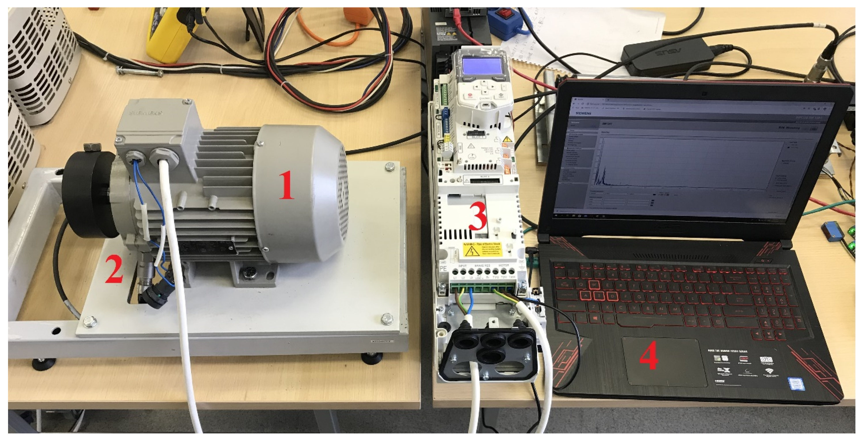
For this test, a test bench was designed. The motor drive part of the experiment is displayed in Figure 1.

In Figure 1, a Siemens asynchronous motor can be seen (marked as number 1), with vibration sensor installed into the bearing housing plate and marked as number 2. This motor was powered from an ABB frequency converter, marked as number 3, and a laptop for signal storage and processing, marked as number 4. The main motor parameters were: Siemens asynchronous motor, 1.1 kW power rating with 2.6 A current, connected as star, cosφ–0.81 and 1415/min revolutions at 50 Hz frequency; efficiency class–IE1–75%. 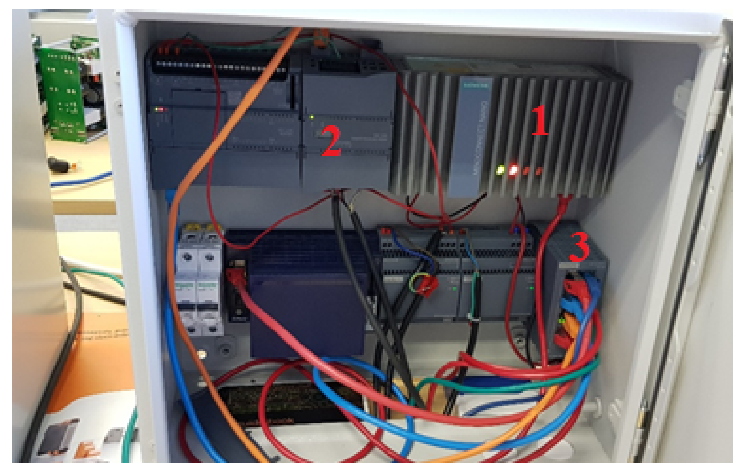The data acquisition part was the same as in [32] and is shown in Figure 2.

The main parameters of measurement and recording equipment that were more noticeable were that the Siemens vibration sensor used was a piezo-quartz recorder with integrated evaluation electronics and had a sensitivity of 100 mV/gn with operating range between 0.5 and 15,000 Hz. Vibration measurement was done at 46 kHz sampling rate, which was the maximum possible of the Siemens monitoring PLC. The communication was done using Profinet and recorded data was uploaded to the cloud by the Siemens measurement PLC using Siemens MindConnect Nano gateway, which was accessible by laptop to retrieve and process. More detailed specifications of the equipment can be found in

Table 1. Training results.

Training	Loss	Sparse Categorical Accuracy	Validation Loss	Validation Sparse Categorical Accuracy
1	0.0410	0.9847	0.3409	0.9067
2	0.0377	0.9887	0.1650	0.9447
3	0.0273	0.9913	0.0959	0.9753

and

Table 2. Summary of testing results for each class.

Condition	Accuracy (CNN)	Accuracy (PCA)
Normal	100%	96.40%
Defective support	98.37%	91.20%
Shaft misalignment	100%	99.20%
Worn-out bearing	97.96%	94.40%
Lost phase	100%	95.60%
Short circuit in winding	87.39%	72.80%

of article [32].

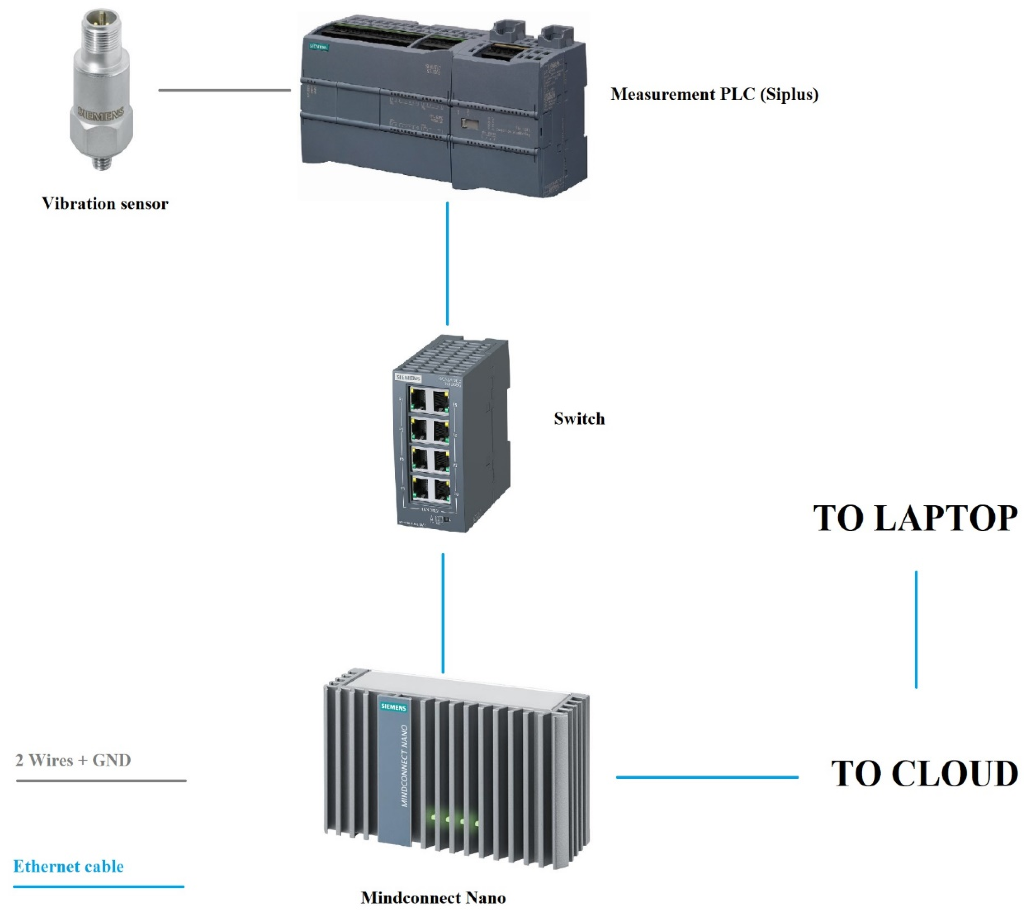
Siemens monitoring PLC, marked 2, and the “Mindsphere” gateway (MindConnect Nano), marked 1, in Figure 2. Everything was connected by Ethernet to a switch which is marked number 3 on the figure. Gateway was connected to the internet to upload the data in audio format, which was then obtained by PC and converted to excel CSV data format. The full layout of the data acquisition part of the experiment is given in Figure 3.

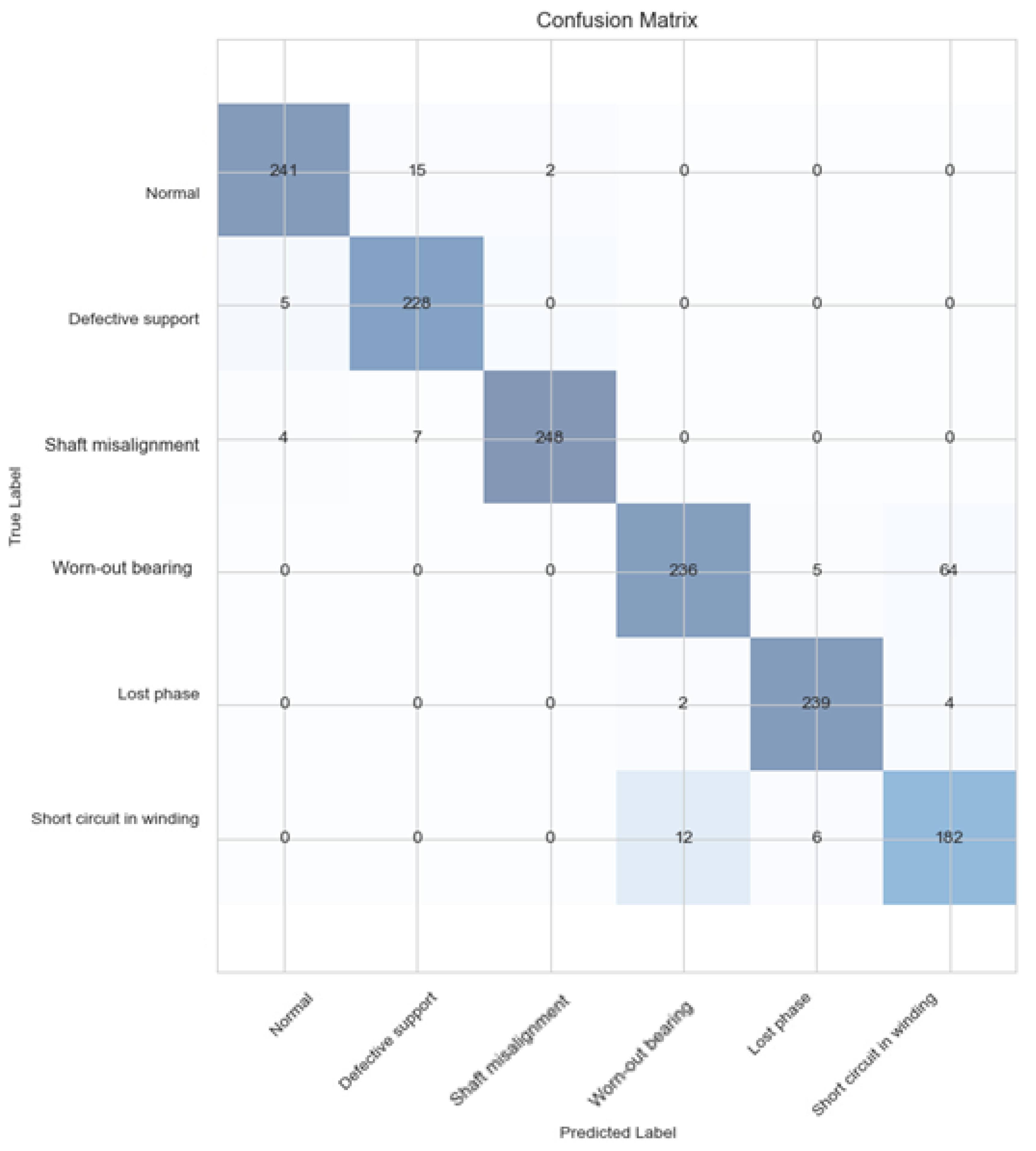
The experiment was done using six different cases of motor condition. This includes class 1 as healthy motor, class 2 as defective support, class 3 as rotor shaft misalignment, class 4 as worn-out bearing, class 5 as lost phase to motor, and class 6 as short circuit in winding. All of the classes were monitored in static conditions for 90 s, and all of the data were uploaded in audio format to the cloud. After downloading the data, they were converted to comma-separated values or CSV format consisting of more than 4,000,000 sample points for each of the class signals, totaling around 24,000,000 sample points between all of the classes. It should be emphasized that in the case of such data proportions as were used for this experiment, feature extraction is a must. This dataset was then used for the training of the classification model described below.

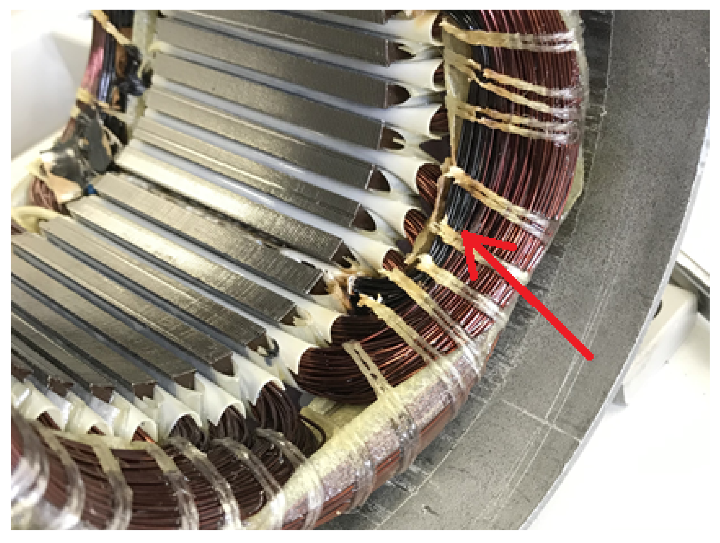
In the case of class 6, where winding was shorted, a resistance of phase 2 winding was reduced by 1 Ω. It was shorted and the resistances were measured using Hioki LCR meter. The resulting resistances were: phase 1–7.86 Ω, phase 2–6.88 Ω, and phase 3–7.87 Ω. The resulting damage of the short circuit is given in Figure 4.

A black burnt winding interturn can be seen in Figure 3 (highlighted in red), which was a result of inhibited short circuit fault. A switch was used to manually short the stator winding.

2.2. Data Acquisition and Standardization

The raw data acquired in the experiment were firstly consolidated into one dataset to prepare it for the standardization process. Then, it was standardized to simplify and improve the feature extraction and training processes. This was done to decrease model bias and speed up neural network convergence. If the training is done on CPU only, data standardization could make a huge difference in training effectiveness. The standardization was applied to the whole 24,000,000 sample point dataset. Standardization was done using mean and standard deviation, using Equations (1) and (2) from [34].

$$\sigma \left(X\right)=\sqrt{Var\left(X\right)}$$

(1)

$$Z=\frac{X-E\left[X\right]}{\sigma \left(X\right)}.$$

(2)

where $\sigma \left(X\right)$—standard deviation, $E\left[X\right]$—expected value (mean of the variable).

After the standardization was applied to the dataset, it was then split into six different datasets separated by the class. The resulting six datasets consisted of 500 different vibration measurement signals for each class. This resulted in a total of 3000 signal measurements used for the training. All of the 500 signals had the same length of 800 sample points. As it can be seen from the size of the dataset, not all the data were prepared for the experiment. This is because different datasets for training and testing are needed. The different data are used to truly test the trained model because if the same data were introduced for the testing as for the training, the model could easily classify the data, because it was the same data it learned from. On the other hand, if completely different data are introduced, the model reaction is tested with the new data. If it can successfully distinguish the classes from the new dataset, then the model is trained successfully and can be used in real scenarios.

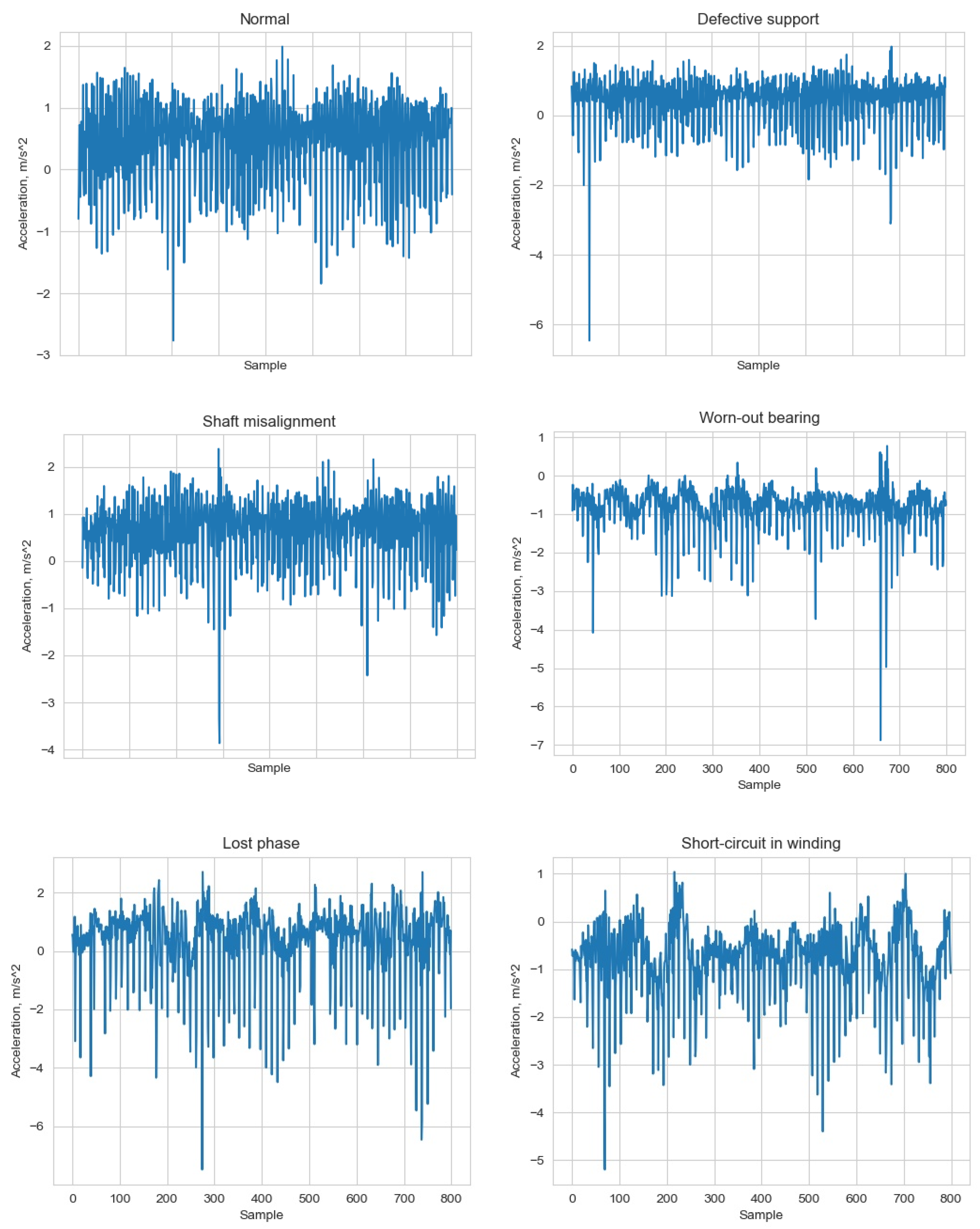
As mentioned above, since 3000 signals were used for all six classes, consisting of 800 measurement sample points each, a total of 2,400,000 sample points between all signals were used for the training, or 400,000 for each training class. This should be enough, because if the datasets are too large, then scalogram resolution must be increased, thus increasing model complexity and computer resources required. In case of low accuracy and high loss, during training, the number of measurement samples can be increased. For the training, 250 signals were used for each class, consisting of the same number of vibration sample points each as in the training dataset. This results in a total of 1,200,000 sample points used for the dataset or 200,000 from each of the classes. The resulting one signal sample of the training dataset for each class is given in Figure 5.

As it can be seen from the samples given in Figure 4, the features were quite distinctive, and each individual training class had different features and patterns exhibited in the examples. However, the model could still have a hard time training with that many features and big datasets could complicate the training process, increasing training time and error. Next, the continuous wavelet transform was applied to the dataset for the feature extraction. This will be explained and discussed in the next section of the article.

2.3. Feature Extraction

After obtaining and preparing the data by standardizing and division to training and testing samples, feature extraction can be done. This was achieved in two parts. The first part was continuous wavelet transform, where morl wavelets were applied, and the second part was where scalograms were acquired from the signals for training.

Complex morl wavelet transform was calculated using Equations (4)–(6) from [11] and window function, known as mother wavelet Ψ(t), was used to calculate each part of the time-domain signal individually. The mother wavelet satisfies (3) from [11]:

$${{\displaystyle \int }}_{-\infty }^{\infty }\Psi \left(t\right)dt=0.$$

(3)

The CWT is expressed by:

$$CWT\left(b,a\right)={\displaystyle \int }F\left(t\right){\Psi }_{b,a}^{*}\left(t\right)dt.$$

(4)

where ${\Psi }_{b,a}^{*}\left(t\right)$. is the conjugate to the mother wavelet function ${\Psi }_{b,a}\left(t\right)$.

The function f(t) is decomposed into a set of basic functions known as wavelets. These wavelets are generated from the mother wavelet by scaling and translation:

$${\Psi }_{b,a}\left(t\right)={\left|a\right|}^{-\frac{1}{2}}\Psi \left(\frac{t-b}{a}\right)$$

(5)

where a is the scale factor or window length and b is the translation factor; the factor ${\left|a\right|}^{-\frac{1}{2}}$ is for energy normalization across different scales.

If the wavelet function in (4) is complex, it is defined as a complex wavelet transformation and it is calculated in (6):

$${\Psi }_0\left(t\right)=\frac{1}{\sqrt{\pi f_b}}\exp \left(2i\pi f_{c}t\right)\exp \left(-\frac{t^2}{f_b}\right).$$

(6)

where $f_b$ is wavelet bandwidth, $f_c$ is wavelet center frequency.

The magnitude squared wavelet transforms of, in other words, scalograms were calculated from the resulting transformed signals using (6) from [35].

$$P_x^W\left(a,b\right)=\left|W_x\left(a,b\right)W_x^{*}\left(a,b\right)\right|.$$

(7)

If the wavelet transforms of two signals x and y are denoted with $W_x\left(a,b\right)$ and $W_y\left(a,b\right)$, the wavelet cross scalogram is defined as (7).

The wavelet transformation uses the mother wavelets to divide a 1D to ND time series or image into scaled components. In this connection, the transformation is based on the concepts of scaling and shifting. Scaling means enlarging or shrinking the signal in time by a factor called scaling factor and shifting means moving differently scaled wavelets from the beginning to the end of the signal. The scale factor corresponds to how much a signal is scaled in time and it is inversely proportional to frequency. This means that the higher the scale, the finer the scale discretion. So, to capture slow changes, the wavelets are stretched, and to capture abrupt changes in the signal, the wavelets are shrunk. The different wavelets in scales and time are shifted along the entire signal and multiplied by its sampling interval to obtain physical significances, resulting in coefficients that are a function of wavelet scales and shift parameters.

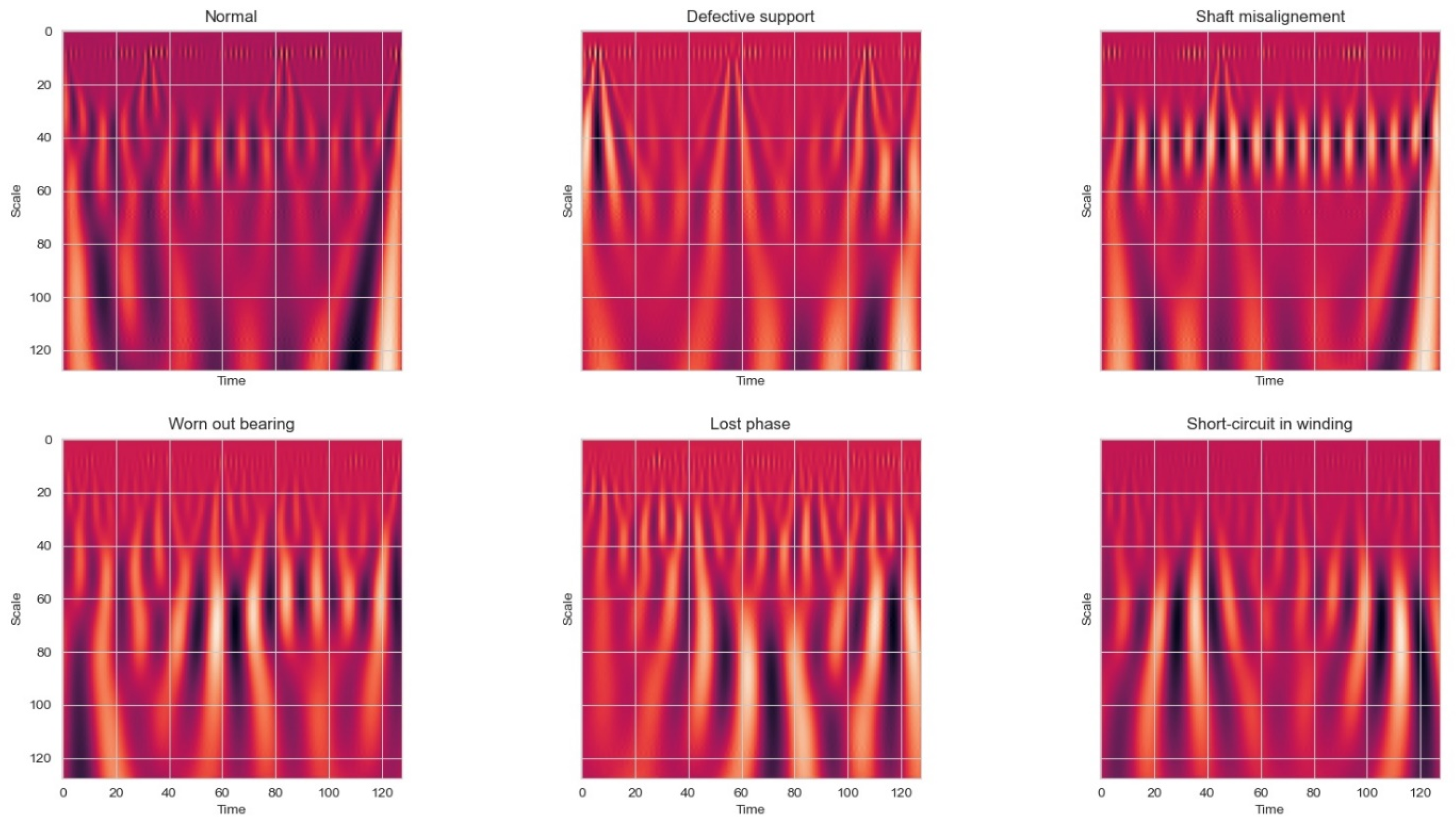
The resulting scalograms are given in Figure 6. The data represented in the figure are from one sample, featuring all of the classes. The same sample was used as for the data represented in Figure 5.

The scalograms in Figure 6 indicate where most of the energy (yellow-white parts in the figures) of the original signal was contained in time and frequency. Furthermore, it can be seen that the characteristics of the signal are now displayed in highly resolved detail. The abrupt changes are often the most important part of the data both perceptibly and in terms of the information that they provide as they are seen in the figures as yellow-white parts.

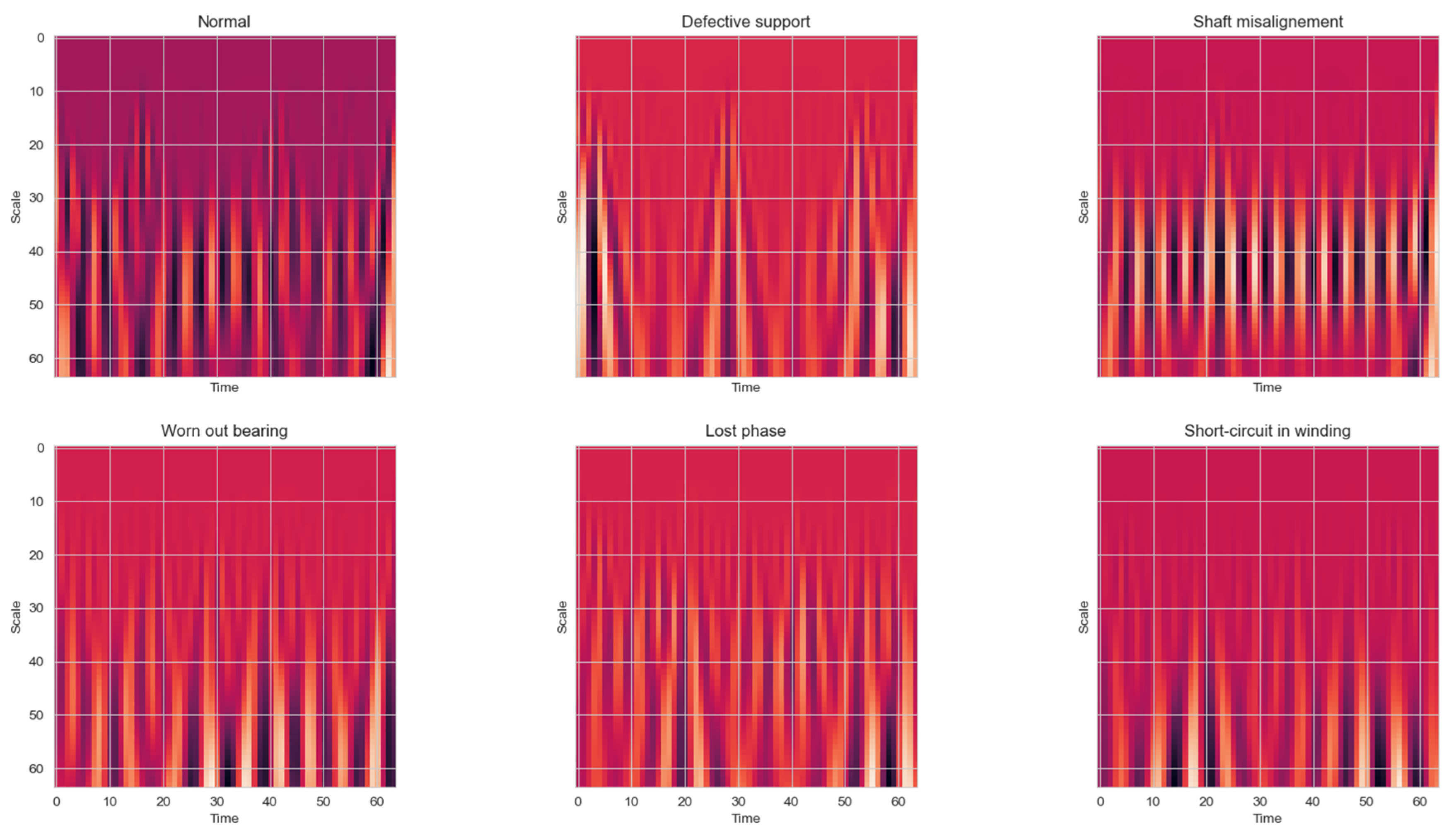
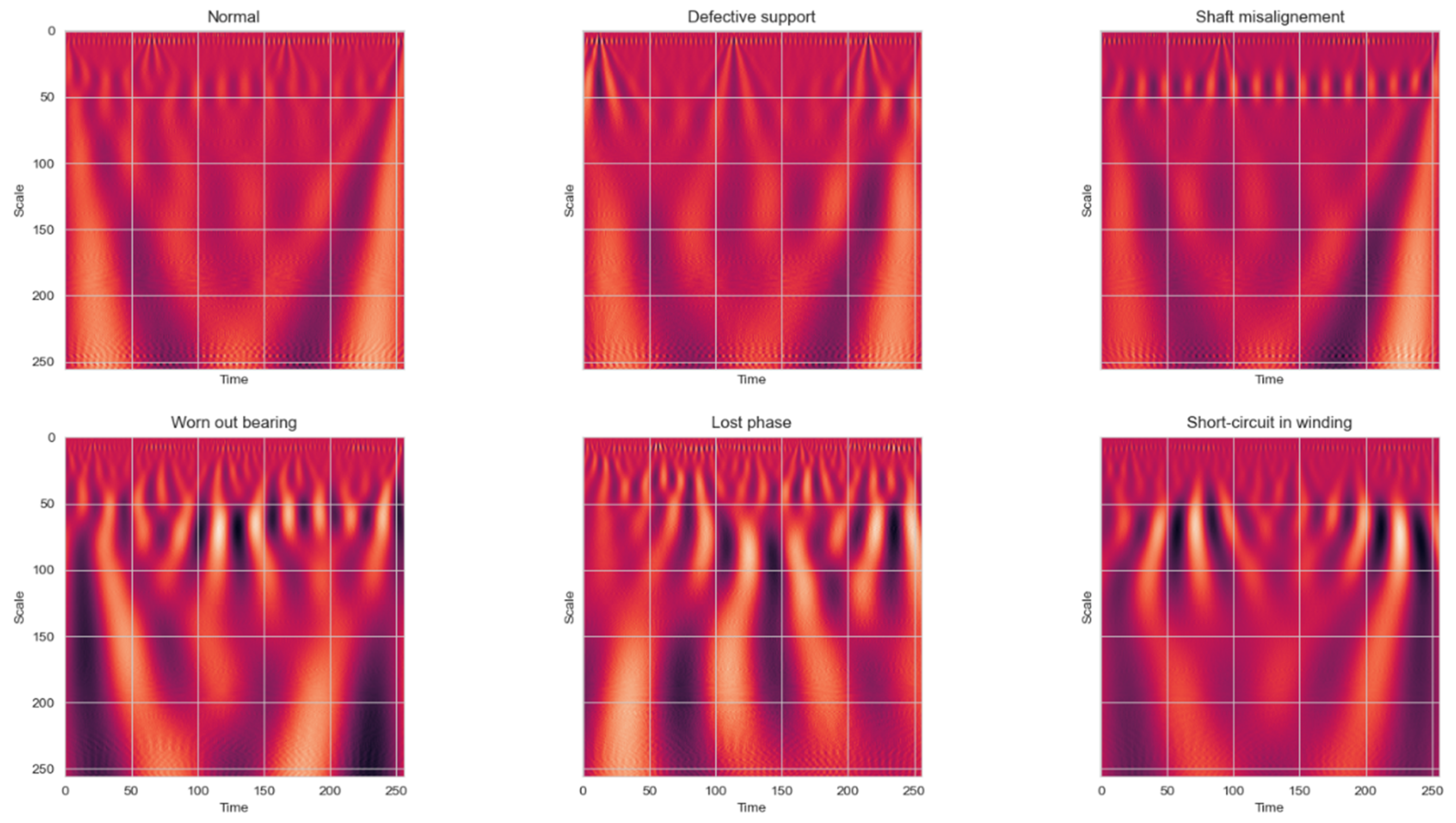
The scalograms were reshaped to fit the resolution (scale) of 128 × 128. The key here is to have as many visible features as possible by using as low a resolution as possible. This is to not overcomplicate the model and to not strain the computer resources. For example, a 64 × 64 scalogram sample is given in Figure 7 and 256 × 256 in Figure 8.

As it can be seen from Figure 7, the scalograms are quite pixelated and are zoomed in, but the training performance in terms of speed was much more increased. A smaller size of scales enables more focus of abrupt changes. As already mentioned, these sudden changes are often the most important characteristics. However, in this case, it can be seen that the zoomed-in scalograms provide less features, while giving more detail to existing ones. Unfortunately, some features do not fit into the graphs as in Figure 6, which can decrease the accuracy of the training.

Otherwise, a wide range of scales as seen in Figure 8 provide more information about slow changes, which can provide a better classification accuracy in case of slower processes recorded. This can be seen in the graphs as the signals are more zoomed out with less visible features in the first three graphs, where probably the vibration features are shorter in time and with lower amplitude. But for the bottom three classes displayed, more features can be seen. Thus, a more complex neural network should be used in that case.

Unfortunately, when dealing with 3000 samples of data measurements, the high-performance computer used could not allocate enough resources for the training and the scalogram calculation itself was increased considerably. So, by trial and error, it was decided to use 128 × 128 scalograms for the training, where most features are visible across all six classes, with the sample displayed in Figure 6.

2.4. Training and Testing Model

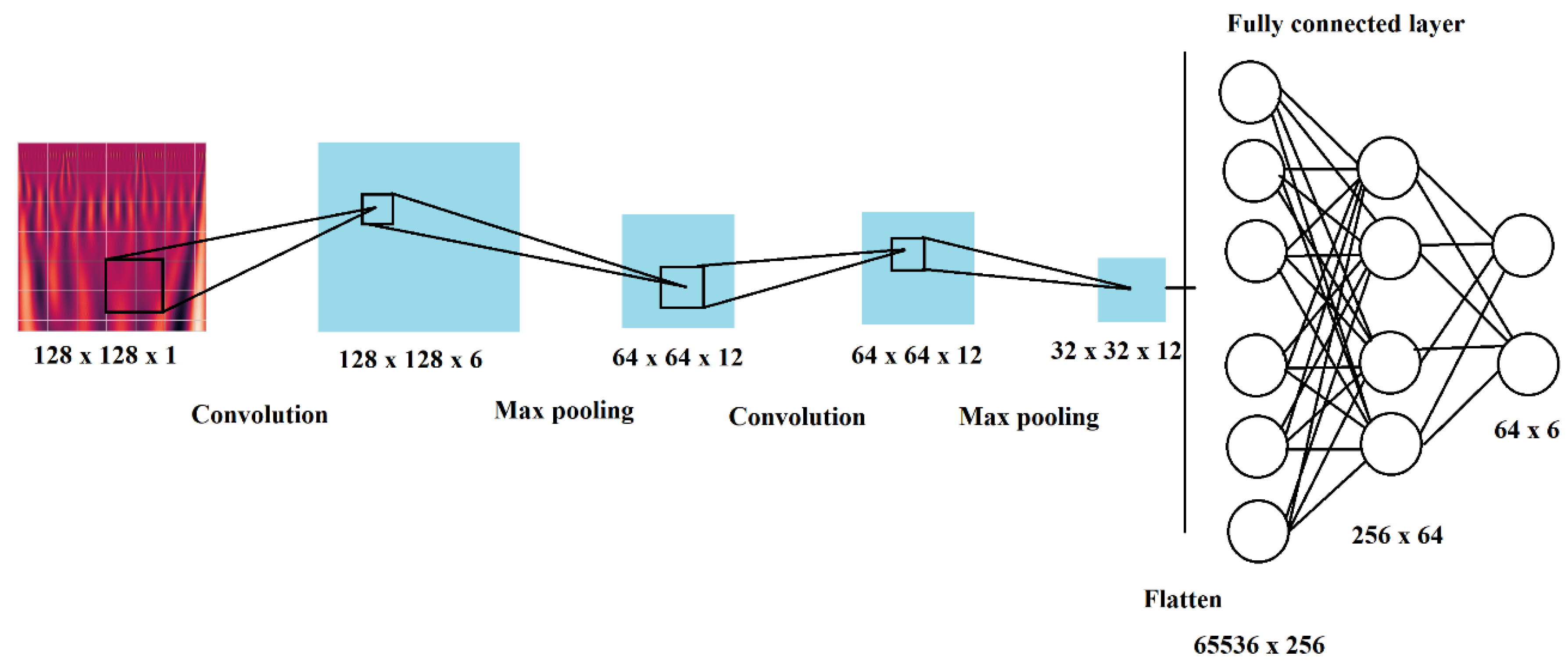
After data preparation, which included standardization and feature extraction using CWT and scalograms, the model could be trained. A CNN LeNet-5 architecture model similar to one in [36] was designed for the training itself. The training model diagram is given in Figure 9.

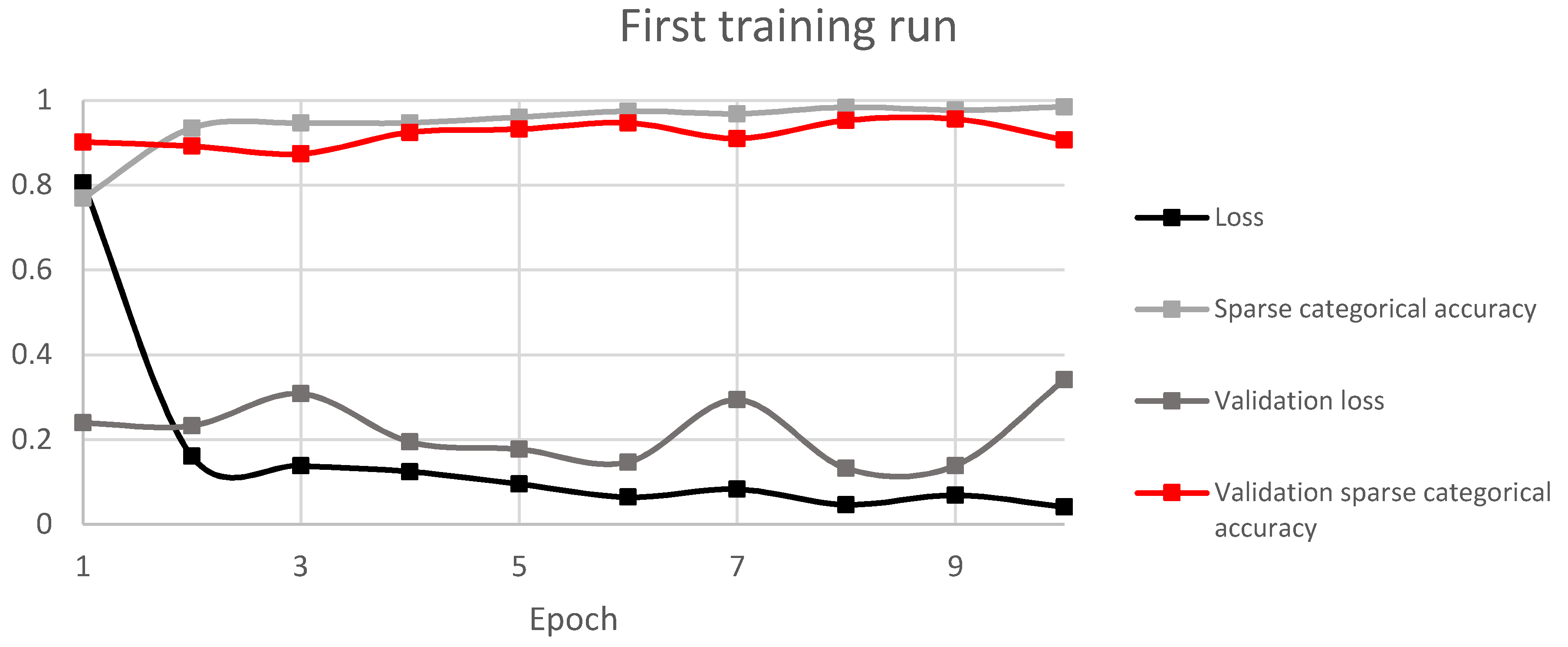
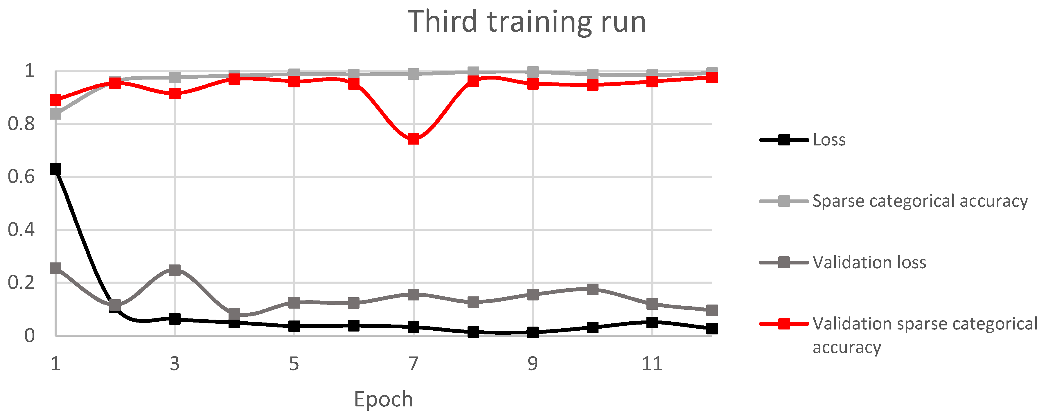
The training was conducted using the model visualized in Figure 8, using a Python TensorFlow plugin. The model consists of inputs as scalograms and four layers of feature maps which include two convolution with 5 × 5 kernel and two max pooling with 2 × 2 kernel layers. After flattening, the fully connected layer consists of two layers and one output–softmax layer. Rectified linear unit (ReLU) activation functions were used to accelerate convergence and increase the performance. The performance was measured using sparse categorical accuracy and loss–sparse categorical cross entropy. Sparse categorical accuracy checks to see if the maximal true value is equal to the index of the maximal predicted value. It is a bit different from categorical accuracy which checks to see if the index of the maximal true value is equal to the index of the maximal predicted value. Training was done in 10 epochs for the first run and 12 epochs for runs 2 and 3, with 20 batch size, which had to be lowered due to the big data size.

The training algorithm is described in Equations (8) through (13) and are described below, for each layer from [37,38]. The equation of convolution layer is represented in Equation (8):

$$a_{i,j}={\left\{f\left({\displaystyle \sum }_{m=0}^{F-1}{\displaystyle \sum }_{n=0}^{F-1}{w}_{m,n}{x}_{i+m,j+n}+b\right)\right\}}_{i=1,2,\dots ,I;j=1,2,\dots ,}$$

(8)

where

• $a_{i,j}$ is the output after convolution,
• b is the offset term from each of the convolutions,
• f() is the activation function,
• F is the size of the convolution kernel.

In this layer, a feature extraction process is conducted. The input matrix is convolved with the convolution kernel in this layer. The activation function expression for the layers is given in Equation (8). A ReLU activation function was used for all the training layers.

$$f\left(x\right)=\max \left(0,x\right)$$

(9)

The pooling layer is used to perform the feature selection process by reducing dimensions of the data and preserving the main characteristics for the data used in the training. One of the most popular methods, maximum pooling, was used for the training. As previously mentioned for maximum pooling, a 2 × 2 kernel was used, meaning that the input feature matrix is reduced by a factor of two in both dimensions. The equation for the pooling layer is given in Equation (9):

$$a_n^l=pool\left(a_n^{l-1}\right)$$

(10)

where

• pool() is the maximum pooling operation,
• $a_n^l$ is the output of the l layer,
• $a_n^{l-1}$ is the output of the formal layer,
• n corresponds to sample number.

After pooling and flattening the last layer of the CNN before the output is a fully connected layer. The output of this layer is given in Equation (10):

$$a_n^l=f\left(w^l·a_n^{l-1}+b^l\right)$$

(11)

where

• l is the output layer for the fully connected layer,
• $w^l$ is the convolutional kernel,
• $b^l$ is the offset term.

Lastly, the output layer, or in other words, the softmax layer, used in this training is given in Equation (11). Output layer number is defined by the number of classes for the classification problem that is being solved, which in this case is six.

$$a_n^L=o_n^v=softmax\left(w^L·a_n^{L-1}+L\right)$$

(12)

where $o_n^v$ is the probability of different classification categories obtained by softmax and it indicates the output probability of the n sample for v different classified categories, which is six. The error formula corresponding to n sample is given in Equation (12):

$$E_n=\frac{1}{2}{\displaystyle \sum }_{v=1}^V{\left|\left|t_n^v-o_n^v\right|\right|}_2^2$$

(13)

where $t_n^v$ is the expected output probability of n sample in v different class categories.

The best performing model was selected by validation sparse categorical accuracy. For that, a small sample was defined as validation data.

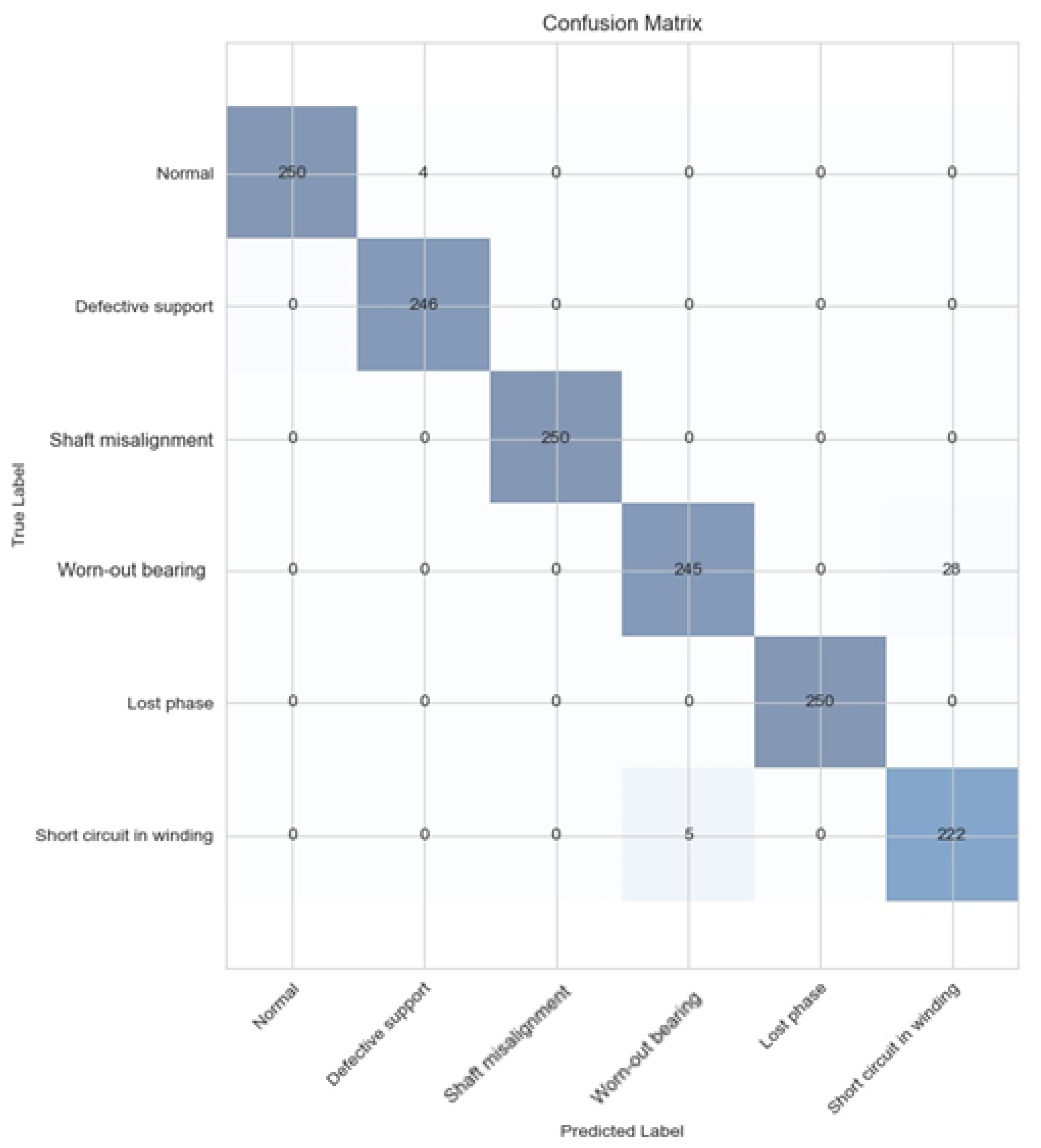
The testing was done with the model by introducing new, unseen test data and testing the classification capabilities. Then, a confusion matrix was plotted with the test results. Test results are described in Section 3.2. Confusion matrix acquisition after training is described more in detail in [32].

2.5. Comparison of Trained Model Performance

For testing if the model was accurate, a more common method was used. A principal component analysis (PCA) algorithm was selected, for its simplicity and accuracy combined with gradient boost decision tree algorithm for classification. For the previous model, 2D images created using CWT were used for the CNN classification model. Here, the most important coefficients per scale were fed to a classifier to acquire features with the highest variation. This time, instead of working with 128 × 128 images, a 128-feature map (1D) after PCA applied was used. Thus, a continuous wavelet transform was applied to the signals and the PCA was applied only to a single component in order to obtain the most significant coefficient per scale. After PCA, the classification was done using gradient boosting, a decision tree-based ensemble machine learning algorithm designed for speed and performance.

The typical PCA algorithm works in this way: calculations of the covariance matrix × of data points are done, then eigen vectors and corresponding eigen values are calculated, then the eigen vectors according to their eigen values are sorted in decreasing order; first, k eigen vectors are chosen and that will be the new k dimensions, and lastly, the original n dimensional data points are transformed into k dimensions.

The calculations for PCA were done using [39]. Firstly, the nonlinear mapping function was defined:

$$\begin{gathered} \Phi :x_d\to F \\ {x}_1,x_2, \dots ,x_m\to \Phi \left(x_1\right),\Phi \left(x_2\right),\dots \Phi \left(x_m\right). \end{gathered}$$

(14)

where

• $\left\{x_i\right\}$ is the input space,
• $\Phi$ is the nonlinear mapping function.

Conditions that data centralization met were defined:

$${\displaystyle \sum }_{\mu =1}^M\Phi \left(x_{\mu }\right)=0$$

(15)

Then, the covariance matrix in feature space F is expressed as:

$$C=\frac{1}{M}{\displaystyle \sum }_{\mu =1}^M\Phi \left(x_{\mu }\right)\Phi {\left(x_{\mu }\right)}^T$$

(16)

The solutions of equations for eigenvalues and eigenvectors are expressed as:

$$Cv=\lambda v$$

(17)

where conditions are satisfied; eigenvalue $\lambda \ge 0$ and $V\in F\left\{0\right\}$.

$$\left(\Phi \left(x_v\right)\times Cv\right)=\lambda (\Phi \left(x_v\right)\times v$$

(18)

Eigen vectors then can be expressed linearly:

$$v={\displaystyle \sum }_{i=1}^M{\alpha }_i\Phi \left(x_i\right)$$

(19)

then:

$$\frac{1}{M}{\displaystyle \sum }_{\mu =1}^M{\alpha }_{\mu }\left({\displaystyle \sum }_{\omega =1}^M(\Phi \left(x_v\right)\times \Phi \left(x_{\omega }\right)\times \Phi \left(x_{\omega }\right)\times \Phi \left(x_{\mu }\right))\right)=\lambda {\displaystyle \sum }_{\mu =1}^M\left(\Phi \left(x_v\right)\times \Phi \left(x_{\mu }\right)\right)$$

(20)

The matrix K of $M\times M$. dimensions can be defined:

$$K_{\mu v}=\left(\Phi \left(x_{\mu }\right)\Phi \left(x_v\right)\right).$$

(21)

and the equation can be simplified:

$$M\lambda K\alpha =K^2\alpha .$$

(22)

The relationship in (22) can be satisfied and the eigenvalue sum including the eigenvector can be calculated from Equation (22), with the projection of eigenvectors on the feature space given in (23).

$$M\lambda K\alpha =K\alpha .$$

(23)

$$\left(v^k\times \Phi x)\right)={\displaystyle \sum }_{i=1}^M{\left({\alpha }_i\right)}^k(\Phi \left(x_i\right),\Phi \left(x\right)).$$

(24)

Substitute for kernel function is defined as:

$$\left(v^k\times \Phi \left(x\right)\right)={\displaystyle \sum }_{i=1}^M{\left({\alpha }_i\right)}^{k}K\left(x_i,x\right).$$

(25)

if ${\lambda }_1\ge {\lambda }_2\dots \ge {\lambda }_M$. is the eigenvalue of the K matrix, and the principal element selection rule is:

$$\left({\displaystyle \sum }_{k=1}^p{\lambda }_k/{\displaystyle \sum }_{i=1}^M{\lambda }_i\right)>E$$

(26)

and if ${\sum }_{\mu =1}^M\Phi \left(x_{\mu }\right)\ne 0$ is adjusted to:

$$\Phi \left(x_{\mu }\right)\to \Phi \left(x_{\mu }\right)-\frac{1}{M}{\displaystyle \sum }_{v=1}^M\Phi \left(x_v\right),\left(\mu =1,\dots ,M\right)$$

(27)

The corresponding kernel matrix can be transformed to:

$$K_{\mu v}\to K_{\mu v}-\frac{1}{M}\left({\displaystyle \sum }_{\omega =1}^M{K}_{\mu \omega }+{\displaystyle \sum }_{\omega =1}^M{K}_{\mu v}\right)+\frac{1}{M^2}{\displaystyle \sum }_{\omega ,\tau =1}^M{K}_{\omega \tau }$$

(28)

Gradient boosting or XGBoost algorithms are some of the most advanced decision tree-based machine learning algorithms. The main idea of the gradient boosting algorithm is to fit the negative gradient of the loss function in repeated iterations after optimizing the empiril loss function, and then use the linear search method to generate the optimal weak learner. The algorithm implements the weak learner by optimizing the structured loss function, and the algorithm does not use the linear search method; it directly uses the first derivative and the second derivative of the loss function. The performance of the algorithm is improved by presorting, weighted quantile, sparse matrix identification, and cache recognition gradient boost. The equations used for gradient boost are given below [40]. Firstly, in Formula 13, model initialization to a constant value is done:

$$F_0\left(x\right)=\arg \hspace{0.17em}\min {\displaystyle \sum }_{i=1}^{n}L\left(y,\gamma \right).$$

(29)

Then, M base learners are generated iteratively:

$$F_{im}=-{\left[\frac{\partial L\left(y_i,F\left(x_i\right)\right)}{\partial F\left(x_i\right)}\right]}_{F\left(x\right)=F_{m-1}\left(x\right)},i=1,2,\dots ,n$$

(30)

Based on the base learner in (14), the optimal ${\gamma }_m$ can be calculated in (15):

$${\gamma }_m=\arg \min {\displaystyle \sum }L(y_i,F_{m-1}\left(x_i\right)+\gamma h_m\left(x_i\right))$$

(31)

Lastly, the model is updated:

$$F_m\left(x\right)=F_{m-1}\left(x\right)+{\gamma }_m{h}_m\left(x\right)$$

(32)

3. Results

3.1. Training

As it was previously mentioned, training was conducted using the Python TensorFlow application. Through trial and error, the best performing parameters (described above) were used for the training. The trial and error trainings were deemed unnecessary to display in the article. The best performing model was obtained with parameters described in the previous chapter. The training itself was conducted a few times to observe if results varied in big proportions. Three training runs were conducted with different accuracy results. The model training processes for all three training runs are given in Figure 10, Figure 11 and Figure 12.

All three training sessions yielded great results. The third training run had the best results of all three with validation sparse categorical accuracy of 97.53. The first two runs were not as accurate, which can be seen in the graphs, especially when looking at errors. The learning rate drop was not introduced, though, because of the high and quite flat third training process. The full training results for all three runs are given in Table 1.

3.2. Testing the Trained Model

After successful training, testing was done by using a different measurement sample, consisting of 1500 samples with 800 signals each as described in Section 2.2. The testing was done only with the best performing training model, which in this case was training 3. The resulting confusion matrix for the third run is shown in Figure 13.

Figure 13 shows how well the classification model can separate different conditions of the asynchronous motor. From the confusion matrix, a conclusion can be made that the actual classes representing six different stages of the motor correspond to trained outputs of the model, which can be seen in the diagonal pane, highlighted in blue, where predicted labels after the training correspond to actual true labels. The only difficulty for the model is distinguishing between worn-out bearing and short circuit in winding; this can be seen for signals that fall not into the highlighted diagonal pane, but can be seen in the matrix, where after training, the model falsely classified the signals not as their true values. In this case, 28 signals from 250 that were from worn-out bearing measurements were falsely assigned to short circuit in winding by the model. Also, four signals were classified as normal, when the support of the motor was loose. It is also worth mentioning that for runs 2 and 3, epoch number was changed from 10 to 12, to give more time for the training.

3.3. Model Comparison

The results of PCA analysis with gradient boost algorithm for classification are given in Figure 14. The testing and training were done with the same data as in the main training. Model comparison was done using the PCA application for coefficient extraction and gradient boost decision tree algorithm for classification as described in Section 2.5 in the methodology section.

As it can be seen from Figure 14, with the more standard model using PCA for the most important feature selection and gradient boost decision tree algorithm for classification itself, the model performed worse than the previous model, with around 6% higher loss in total. Using this model, none of the classes were accurately classified by 100% as in the previous model. The hardest class to accurately classify was short circuit in winding, the same as in the previous model, but now only half of the signals that were of this class were falsely predicted as other classes, most of which were the worn-out bearing class. It is worth mentioning that for this training and testing, only one run was needed, because unlike CNN, PCA and gradient boost always return the same result when conducting the training with the same parameters.

The full summary of testing results for each class individually with comparison to the PCA method is given in Table 2.

4. Conclusions and Discussions

For this article, an accurate and fast method for multiple fault identification for an asynchronous motor was proposed. This model was proven to be 97.53% accurate at classifying all the motor conditions to six different classes including bad bearings, loose mounting, rotor eccentricity, lost phase to motor, and short circuit in stator winding. The features were so detailed because of advanced vibration sensors and feature extraction methods used, that it could distinguish 1 Ω difference in stator winding from vibrations.

The model architecture used in the training was much more successful than other popular and modern methods such as PCA with gradient boost decision tree (XGBoost) algorithms for classification, achieving 6% more accuracy.

The training was very fast and effective, as it took only 2–3 min for full training on GPU with quite a large dataset and only around 5 min training on CPU, which for deep networks is substantial. This was increased considerably from the long short-term memory network used in a previous article [32]. All of this is because of thorough data preparation, including standardization, CWT, and scalogram graphs used before the CNN was applied.

This model can be further enhanced to include more classes, such as broken rotor bars, overheating, and so forth. This would lead to a fully self-diagnosing electric motor that can operate autonomously for long periods of time. The cost of this monitoring system would be substantially less than other conventional methods when utilizing only one vibration sensor to detect mechanical and electrical faults.

This is the first part of planned two-part research. For the next article, the authors will apply this modified model to a frequency converter powered asynchronous motor in dynamic conditions, in order to detect the faults at different speeds, thus fully utilizing the CWT potential.