Do Tense Geopolitical Factors Drive Crude Oil Prices?


1
School of Marxism, Hunan Institute of Technology, Hengyang 421001, China
2
Guangzhou Institute of International Finance, Guangzhou University, Guangzhou 510405, China
3
School of Economics and Commerce, South China University of Technology, Guangzhou 510006, China
4
Accounting and Financial Management, Portsmouth Business School, Portsmouth PO1 3DE, UK
*
Authors to whom correspondence should be addressed.
Energies 2020, 13(16), 4277; https://doi.org/10.3390/en13164277
Submission received: 17 July 2020
/
Revised: 15 August 2020
/
Accepted: 17 August 2020
/
Published: 18 August 2020
(This article belongs to the Special Issue Global Market for Crude Oil)
Abstract
:Geopolitical factors are considered a crucial factor that makes a difference in crude oil prices. Over the last three decades, many political events occurred frequently, causing short-term fluctuations in crude oil prices. This paper aims to examine the dynamic correlation and causal link between geopolitical factors and crude oil prices based on data from June 1987 to February 2020. By using a time-varying copula approach, it is shown that the correlation between geopolitical factors and crude oil prices is strong during periods of political tensions. The GPA (geopolitical acts) index, as the real factor, drives the rise in prices of crude oil. Moreover, the dynamic correlation between geopolitical factors and crude oil prices shows strong volatility over time during periods of political tensions. We also found unidirectional causality running from geopolitical factors to crude oil prices by using the Granger causality test.
1. Introduction
This paper examines the dynamic correlation and causality between geopolitical factors and crude oil prices in different political environments. Although there are many studies discussing the impact of extreme political acts on crude oil prices [1,2,3,4], we use the GPR (geopolitical risk) index and its sub-indices, GPT (geopolitical threats), and GPA (geopolitical acts), constructed by Caldara and Iacoviello [5], Brent and West Texas Intermediate (WTI) to study the dynamic correlation between geopolitical relations (tense and moderate) and crude oil prices (see Appendix A for an explanation of the nomenclatures). Additionally, this study further examines whether there is a causality between geopolitical factors and crude oil prices. To the best of our knowledge, this is the first time that the GPR index is used to examine causality between geopolitical factors and crude oil prices.
The background and importance of this study are that international crude oil prices are always closely related to extreme political events. With the global spread of the COVID-19 virus in 2020, demand for crude oil has been hit hard, and international crude oil prices have fallen off a cliff since March. Many studies proved that geopolitical factors have an important impact on crude oil prices, such as following Gulf War and the 9/11 attack. For instance, Zhang et al. [6] and Dey et al. [7] examined the impact of extreme political events on crude oil prices and suggested that people consider the impact of extreme political events when predicting oil prices. The fluctuations of international crude oil prices will seriously affect the real economy and hinder the stability of the financial system, and may even lead to systemic risks in global financial markets [8,9,10,11]. Therefore, our study focuses on the relationship between geopolitical factors and crude oil prices, which has important implications for some Arab economies and/or for the major oil-exporting countries.
Transmissions of geopolitical factors to the oil market are the result of the action of many channels. The following three important channels are used as examples to show how geopolitical factors affect crude oil prices. The first channel is that geopolitical risks have a positive impact on energy conversion, thereby decreasing crude oil prices. The main reasons for the decline in crude oil prices lie in fuel substitution [12,13]. The second channel is that conflict threats have a negative impact on investor sentiment [14], thereby affecting crude oil prices. A study shows that investor sentiment is highly correlated with the yield of crude oil prices [15]. Therefore, investor sentiment is an important channel for geopolitical factors to affect crude oil prices. The third channel is that conflict threats may have a serious impact on oil production and demand, which is ultimately reflected in crude oil prices [16,17,18]. For example, Salameh [1] pointed out in his research that extreme political events in the Iraqi region will reduce the speed and scale of oil extraction.
Since the study of Caldara and Iacoviello [5], many papers have used the geopolitical risk (GPR) index. This index developed by Caldara and Iacoviello is considered comprehensive because it includes terror attacks and other forms of geopolitical tensions [19,20]. They also constructed a series of the GRP sub-indices, two of which are a geopolitical threats (GPT) index and a geopolitical acts (GPA) index. Many empirical studies tested the effect of the GPR index and its sub-indices on financial markets. Empirical research by Aysan et al. [21] found that the GPR index has a certain predictive ability on returns and the volatility of Bitcoin, and confirmed that Bitcoin can become a hedging tool for GPR. Other than this, the impact of the GPR index on the stock market, international crude oil, government investment, and international trade is a part of a broad, ongoing controversy [19,22,23,24]. As a further study of the GPR index, Demiralay and Kilincarslan [25] pointed out that only geopolitical events, i.e., GPA, can hurt tourism, whereas GPT has no significant impact on tourism. Mei et al. [26] also found that GPA has a better prediction effect on the long-term volatility of oil futures compared with GPT.
Some existing studies explored varying the Granger causality of rising oil prices. However, this study divides the multivariate causal linkage of rising oil prices into the following two categories. The first category is the bidirectional causal linkage of oil price rising. Benhmad [27], for example, pointed out a major finding that oil price is the Granger cause of the dollar exchange rate. Similarly, the dollar exchange rate is also the Granger cause of the oil price for the long term. Empirical research by Zhong et al. [28] and Wolfe and Rosenman [29] showed the bidirectional causal relationship between oil and natural gas futures prices. The second category is the unidirectional causal linkage of rising oil prices. Lee and Chiu [30] confirmed that oil prices have a unidirectional causal relationship with real income and nuclear energy consumption. Similarly, a number of empirical studies supported the unidirectional causal link between oil prices and agricultural product prices [31], precious metals [32], renewable energy [33], monetary policy [34,35,36,37] and the Renminbi (RMB) exchange rate [38].
Our findings showed that the correlations between geopolitical factors and crude oil prices are greater when extreme political events happened. In addition, the dynamic correlation coefficient of GPA and crude oil prices is not always negative. The dynamic correlation between geopolitical factors and crude oil prices shows strong volatility during periods of political tension. Finally, the results revealed that there is unidirectional Granger causality running from geopolitical factors to crude oil prices in the full sample period.
The innovation of this study is that we tested the correlation between geopolitical risks and crude oil prices in extreme political environments. In addition, we also studied the correlation between the GPR sub-indices and crude oil prices. Finally, our results showed that there is a unidirectional causality running from geopolitical factors to crude oil prices.
The main contributions of this paper can be summarized as follows: First, this study utilizes a time-varying copula approach to examine the dynamic correlation between the GPR index and crude oil prices. The time-varying copula approach is better than the wavelet analysis method used by Su et al. [39] to capture the correlation in an extremely political environment (upper-lower tail correlation) [40,41], which can describe the relationship between the GPR index and crude oil prices in extreme geopolitical environments. Second, the unique results of this paper showed that only a rise in the GPA index can significantly increase crude oil prices, although GPR (or GPT) and crude oil prices generally move together in the same direction (co-movement exist). Further, there is a unidirectional causality running from geopolitical factors to crude oil prices.
The theoretical and practical implications of this paper can be summarized as follows: First, this paper enhances the understanding of international crude oil price fluctuations by examining the dynamic correlation between the GPR index and crude oil prices. In particular, this paper analyzes the impact of war or terrorist activities on crude oil prices and provides new evidence that geopolitical factors affect crude oil prices. Second, an interesting finding from our analysis is that actual extreme political events will drive crude oil prices. The findings of this paper are relevant to stakeholders as they provide stakeholders with effective measures to prevent crude oil price fluctuations.
2. Methods and Data
2.1. Time-Varying Copula
Our motivation for selecting the time-varying copula model is that the correlation between the geopolitical risk and the price of crude oil in extreme environments requires special attention. The reason is that in a relatively stable political situation, geopolitical risks will not significantly change the trend of international crude oil prices, but the upper and lower tails of the distribution of geopolitical risk index (referring to the period of extreme political events) are more and more closely related to the fluctuation of crude oil prices.
Economists mostly use the wavelet analysis method, a family of the GARCH (generalized autoregressive conditional heteroscedasticity) model, and a copula approach to capture the correlation between two variables. The wavelet approach has great advantages in dealing with non-stationary information and it can deal with frequency and time information. Thus, the wavelet approach is very common when dealing with the correlation of frequency information of non-stationary time series [41]. The DCC-GARCH (dynamic conditional correlational-generalized autoregressive conditional heteroscedasticity) model decomposes the covariance matrix into a conditional standard deviation and correlation matrix through orthogonal basis decomposition, thereby obtaining the dynamic correlation coefficients between time series [42]. This process needs to satisfy the conditional heteroscedasticity (ARCH effect) of variables. The correlation of an extremely political environment (upper–lower tail correlation) is particularly important when describing the dynamic correlation between the GPR index and crude oil prices. However, neither the wavelet analysis method nor the family of the GARCH model can capture the tail correlation of the GPR index and the crude oil price distribution. To solve these defects, we used the time-varying copula approach to measure the correlation between geopolitical factors and crude oil prices.
In this paper, we focus on the dynamic correlation between the GPR index and crude oil price ( and , respectively). According to Sklar’s theorem, the bivariate joint distribution for the GPR index and crude oil prices can be represented as a copula function after transforming marginal distributions into uniform distributions [43].
Therefore, the bivariate joint distribution of the GPR index and crude oil price can be expressed as:
where and , and is a copula function that describes the correlation between the GPR index and crude oil price.
The density function of the copula is . Thus, the bivariate joint probability density of the GPR index and crude oil price ( and ) is as follows:
where and are the marginal densities of the GPR index and crude oil price, respectively ( and ).
According to Sklar [43], an n-dimensional joint distribution can be decomposed into its n-univariate marginal distributions and an n-dimensional copula. Patton [44] showed that the upper–lower tail correlation of the GPR index and crude oil price is given for the copula as:
where .
The normal (Gaussian) copula used in this study and its correlation parameters are briefly presented below. The normal copula density is given by:
The normal copula shown in Formula (5) can measure the static correlation, but does not allow for time-varying correlation. Following Patton [44], for the Gaussian copulas we specify the linear correlation parameter as , in order to evolve in time according to an autoregressive (AR) moving average (MA) process, namely ARMA (1,q), as follows:
where is the modified logistic transformation, , and the correlation parameter is characterized by the constant , by the autoregressive term and by the average product over the last observations of the transformed variables, i.e., .
2.2. Marginal Distribution
The GPR index and crude oil price went smoothly after the first-order difference (stability test results can be provided upon request). Thus, this study adopted the widely used ARIMA (autoregressive integrated moving average) model. The model is an extension of the ARMA model. The model is transformed into a stationary series after -order difference, which becomes an model. The basic form of the ARIMA model can be written as:
where represents the GPR index (or crude oil price) after -order differential conversion and represents the random error of the moment. At the same time, is an independently distributed white noise series and obeys a normal distribution with a mean of zero and a variance of .
Given the GPR index (or crude oil price) , the model can be written as:
where represent a constant, represent the ARCH component and represent the GARCH component. The number of lags is selected according to the akaike information criteria (AIC).
2.3. Estimation
This study used the two-stage maximum likelihood (ML) method used by Patton [44] when estimating Copula parameters. The following briefly introduces this parameter estimation method. The log-likelihood function can be written as:
where and are the parameters of the marginal distribution of and , respectively, is the copula density parameter and is the joint density parameter.
The two-step inference for the margins procedure was adopted. First, the GPR index and the marginal distribution of crude oil prices are estimated as follows:
where .
Second, the correlation coefficient between the GPR index and crude oil price is obtained by estimating the copula function:
where and .
2.4. Variables and Data Source
This study sought to investigate the basic question raised earlier regarding the relationship between geopolitical risks and crude oil prices. For this purpose, the GPR measured by Caldara and Iacoviello [5] can be used as a proxy indicator of geopolitical risk. Monthly data for geopolitical risk index are available for download from the website https://www.matteoiacoviello.com/gpr.htm. There are two developed variants of the GPR indices, the GPT and GPA indexes, which we used in our study to investigate the relationship between geopolitical risk and crude oil prices. The GPT index is constructed by searching articles that include words in the groups directly mentioning risks, while the GPA index searches only for the groups directly mentioning adverse events. In addition, crude oil price can be explained by Brent and WTI spot prices based on most of the literature [45,46,47]. We obtained monthly crude oil price data through the US Energy Information Administration (http://www.eia.doe.gov). According to the availability of crude oil price data, the time dimension of the data selected in this study is from June 1987 to February 2020. Table 1 shows the descriptive statistical results of the variables involved in this study.
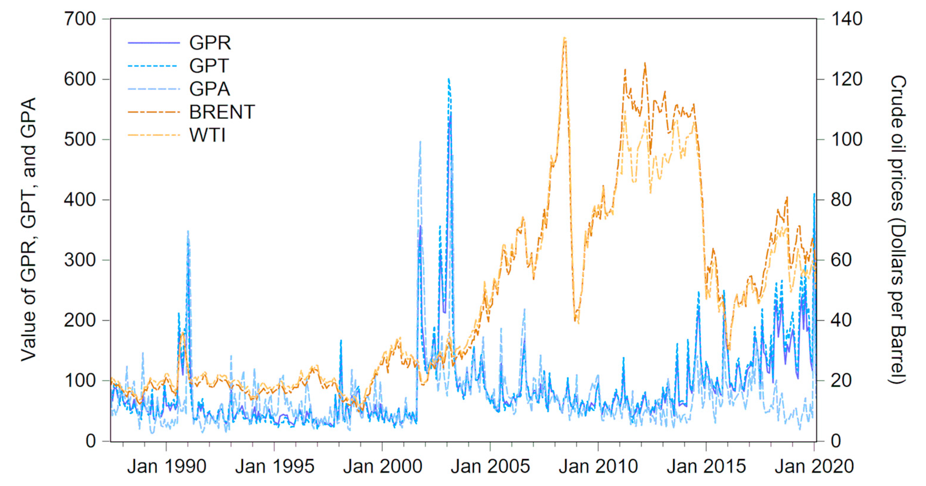
Table 1 reports the descriptive statistics of all variables. From all observations (overall panel), the average GPT value was 88.421, which is greater than the average GPA value of 72.689. This result shows that risk events are more directly mentioned in newspapers relative to adverse events. The kurtosis values of the three indices representing geopolitical risk are very large, indicating that their distribution is more peaked than the Gaussian distribution and shows non-normal characteristics. The statistical values of Brent and WTI are very similar, indicating that whether Brent or WTI represent the international crude oil price, there will be no significant difference in the empirical results. The tension panel presents descriptive statistics for the periods of geopolitical tension and the stabilization panel is for the periods of geopolitical stabilization. For detailed rules on the division of periods of geopolitical tension and stabilization, please refer to Section 4.1 of this paper. At the same time, we also plotted geopolitical risk indexes (GPR, GPT and GPA) and international crude oil prices (BRENT and WTI), as shown in Figure 1.
Since 2015, the correlations between geopolitical factors and international crude oil prices has been continuously strengthened. As shown in Figure 1, the GPR index (including GPT and GPA) and crude oil prices reached a peak at the same time around 1991. During this period, geopolitical factors and international crude oil prices presented similar historical trends. Subsequently, around the 9/11 event, the GPR index (including GPT and GPA) reached its highest values. However, crude oil prices experienced only small fluctuations during this period. Between 2007 and 2015, crude oil prices showed extreme volatility, especially at the end of 2008. Crude oil price dynamics during this period may have little relevance to adverse political events. After 2015, the frequency of adverse events became higher and higher, and crude oil prices also showed a trend similar to the GPR index. Therefore, we initially believe that the relationship between geopolitical factors and international crude oil prices has continued to strengthen since 2015.
3. Empirical Results
3.1. Marginal Distribution Model Results
The marginal models (Formulas (7)–(9)) are estimated by taking different combinations for the lags values, ranging between zero and four, and by selecting the most appropriate - specification with skewed t-distribution according to the AIC values (the best model is the one which minimizes the AIC value). The results of AIC show that the best model for fitting the marginal distribution is . Table 2 presents the parameter estimates for the marginal distribution models.
The results showed that most of the parameters of were statistically significant. This shows that the model is suitable for fitting the marginal distribution of the GPR, GPT, GPA, Brent and WTI series. In addition, the parameters and of the GARCH model were statistically significant for all series (the parameter that fits the marginal distribution of GPA was an exception), which shows that GPR, GPT, BRENT and WTI all have a volatility clustering effect. As was close to 1, this indicates that the shock was quite persistent to the GPR, GPT, GPA, Brent and WTI series [48,49]. We performed autocorrelation and partial autocorrelation tests on the standardized residuals obtained by fitting the marginal distribution of the GPR, GPT, GPA, BRENT and WTI series. The results showed that the model has basically eliminated the autocorrelation, partial autocorrelation and the conditional heteroscedastic effect of the GPR, GPT, GPA, Brent and WTI series (the results are available upon request from the authors). Through the use of the model to filter the data, a residual series with no sequence correlation and no heteroscedasticity was obtained. Finally, we used probability integral transformation to make these residual series obey the 0–1 distribution.
3.2. Dynamic Correlation between GPR and Crude Oil Prices
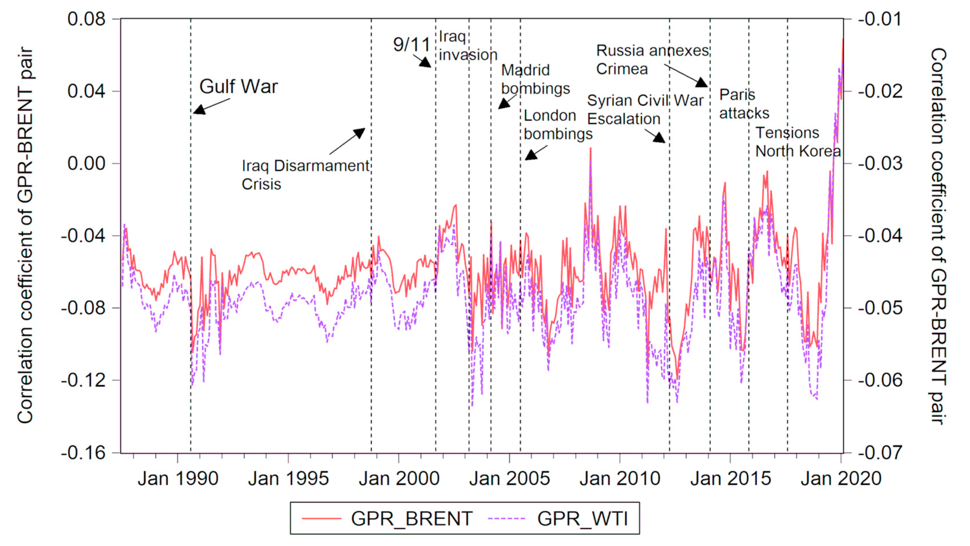
Based on the time-varying copula model, this study estimated the dynamic correlations between the full sample GPR index and crude oil prices from June 1987 to February 2020. Figure 2 presents the dynamic Kendall’s coefficients of the GPR-Brent pair and GPR-WTI pair. The dynamic Kendall’s tau coefficients were used to assess the strength of dynamic correlations between the GPR index and crude oil prices.
During periods of extreme political acts, the correlations between geopolitical factors and crude oil prices were greater than any other period. The dynamic Kendall’s coefficients of the GPR-Brent pair and GPR-WTI pair reflect changes in the correlations between geopolitical factors and international crude oil prices, including the correlation after the unexpected Gulf War in August 1990 and 9/11 events. The dynamic correlation coefficient of geopolitical risk and Brent or WTI fluctuated around −0.05. From the dynamic Kendall’s coefficients, this dynamic correlation does not impose any a priori opinion on whether geopolitical factors are driving crude oil prices upward. However, after the Gulf War (2 August 1990–28 February 1991), the dynamic Kendall’s coefficients of the GPR-Brent pair and GPR-WTI pair were −0.104 and −0.061, respectively. The correlation between geopolitical factors and crude oil prices at this point in time was the minimum during the period 1990–2000, which indicates the strongest negative correlation. After the 9/11 event, the dynamic Kendall’s coefficients of the GPR-Brent pair and GPR-WTI pair were −0.065 and −0.048, respectively. After the extreme events of Iraq’s invasion in 2003, the dynamic Kendall’s coefficients of the GPR-Brent pair and GPR-WTI pair reached the minimum values during the sample period, −0.104 and −0.064, respectively. With the frequent occurrence of extreme events in the early 21st century, dynamic correlations between the GPR index and crude oil prices have been detected with a large number of jumps. The extreme events that occurred in the early 21st century include the 9/11 event (11 September 2001), the Iraq invasion (20 March 2003), the Madrid bombings (11 March 2004), the London bombings (7 July 2005), escalation of the Syrian Civil War (2012–2013), Russia’s annexation of Crimea (February and March 2014), the Paris attacks (13 November 2015), and North Korea tensions (2017–2018). During these extreme events, the correlation between the geopolitical risk index and crude oil prices reached its peak. This means that before and after extreme events, the correlations between geopolitical factors and crude oil prices were enhanced. It could be the case that some extreme geopolitical events are severe enough to have repercussions on global economic policy uncertainty through trade linkages, international capital flows, and confidence channels [11,50,51].
To highlight the advantage of time-varying copula in calculating the correlation between geopolitical factors and crude oil prices, this paper also gives the results of DCC-GARCH and wavelet coherence analyses, as shown in Figure 3 and Figure 4, respectively.
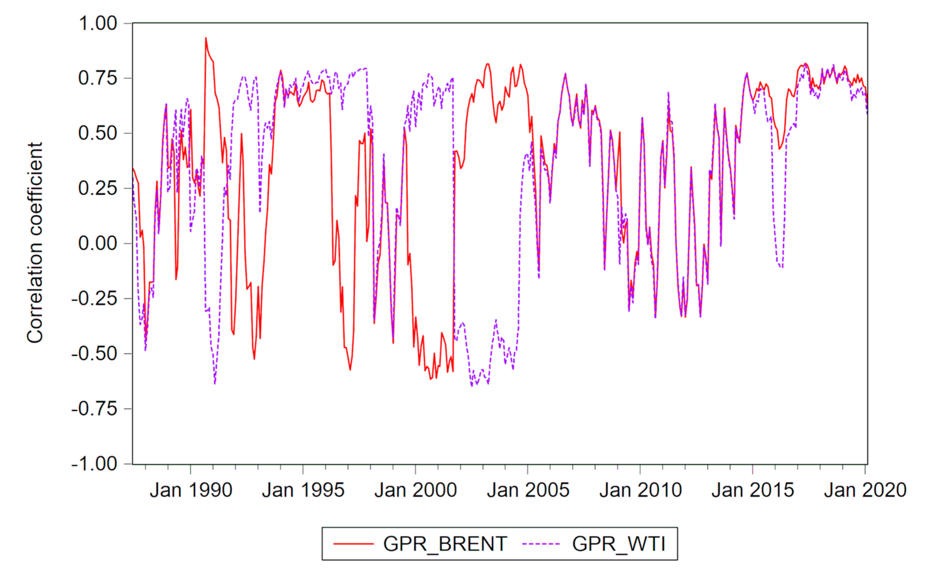
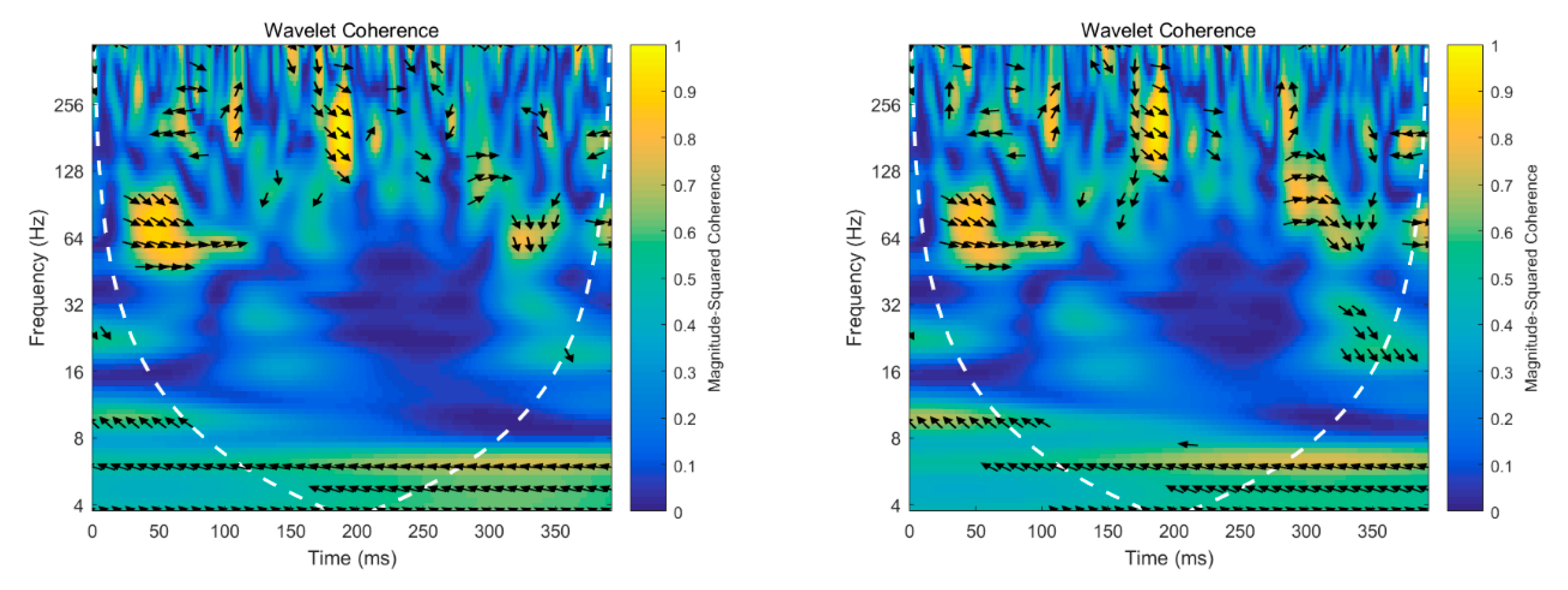
Figure 3 shows the results of dynamic conditional correlations between the GPR index and crude oil prices calculated by the DCC-GARCH model. The dynamic conditional correlations of the GPR-Brent pair and GPR-WTI pair showed a large deviation between 1990 and 2005. These two dynamic conditional correlations coefficients even showed opposite trends. The reason may be that the DCC-GARCH model needs to estimate a large number of parameters when calculating the correlation, so that the results are prone to unavoidable errors. However, the dynamic correlation coefficient shown in Figure 2 is calculated by the time-varying copula, which is a non-parametric approach. The copula approach can effectively measure the correlation between the upper and lower tails of two distributions. In other words, the copula accurately measured the correlation between geopolitical factors and crude oil prices in extreme environments. Figure 4 shows the results of wavelet coherence between the GPR index and crude oil prices. Wavelet coherence analysis provides information on the correlation between the GPR and crude oil prices at different frequencies. Similarly, the DCC-GARCH and wavelet coherence analyses failed to capture the asymmetric correlation between the upper and lower tails of the GPR and crude oil price distribution. Therefore, this study used a time-varying copula to better describe the dynamic correlation between the GPR and crude oil prices.
3.3. Dynamic Correlation between GPR Sub-Indices and Crude Oil Prices
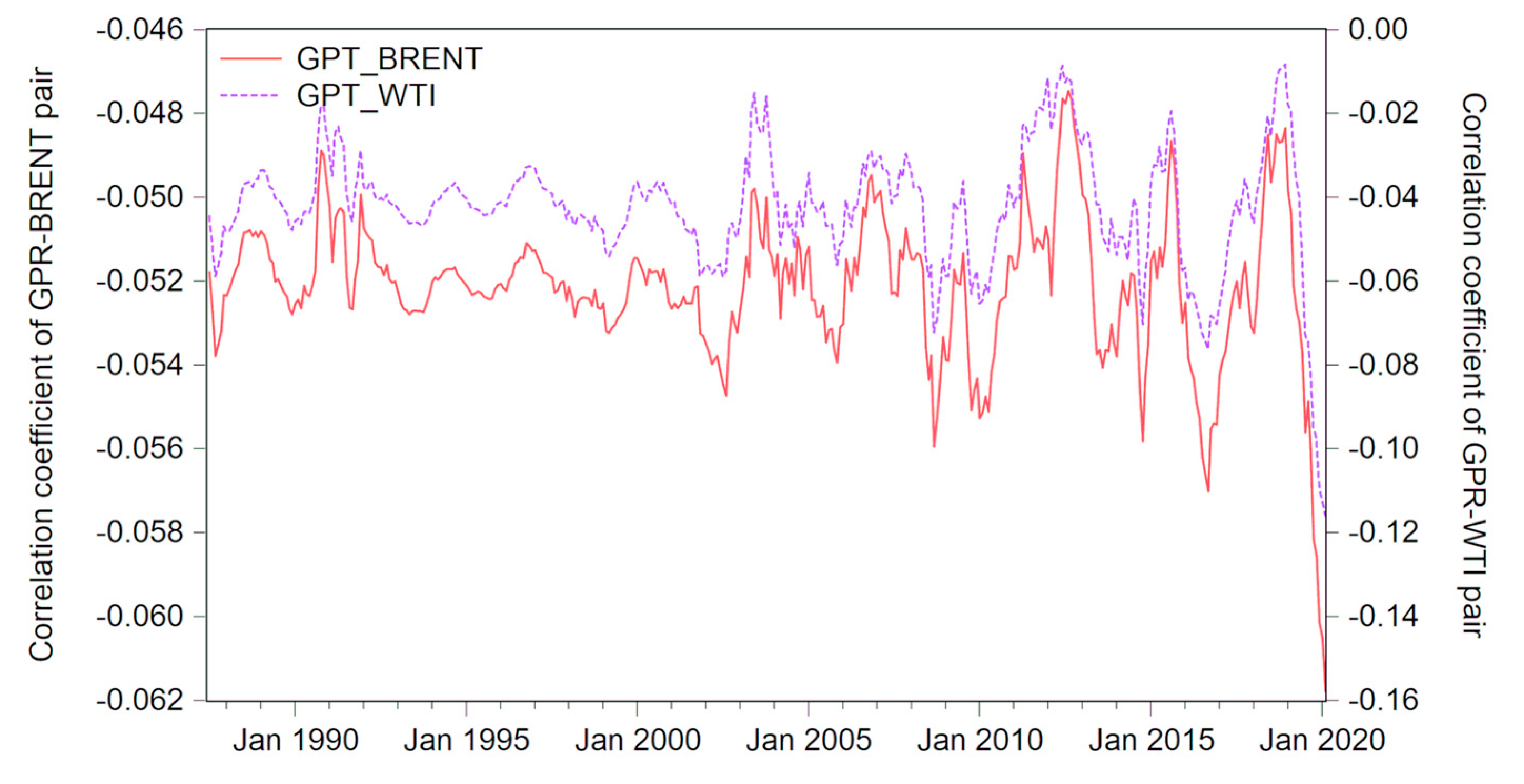
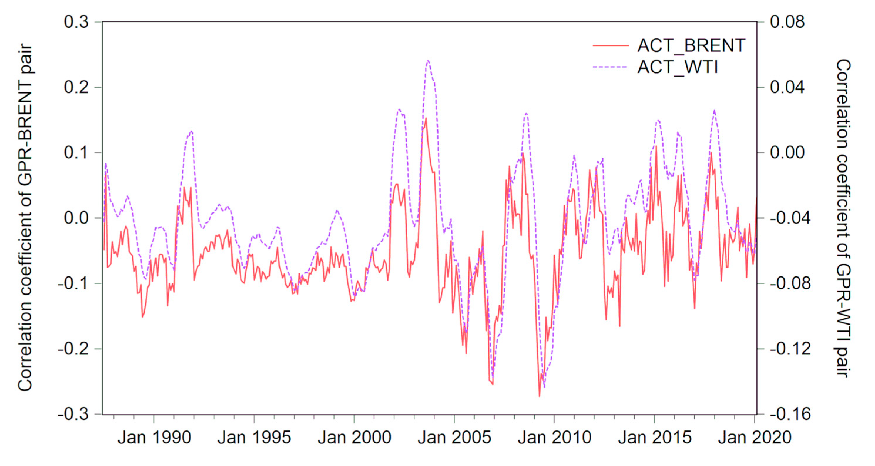
The GPR index can be further decomposed into two sub-indices, that is, whether the news vocabulary of geopolitical risks is related to potential risks or actual adverse events. After verifying the dynamic correlations between the GPR index and crude oil prices, this study estimated the dynamic correlation between the GPT indices and crude oil prices under the full sample. The dynamic Kendall’s coefficients of the GPT-Brent pair and GPT-WTI pair are depicted in Figure 5 (Upper). At the same time, this study also estimated the dynamic correlation between the GPA indices and crude oil prices under the full sample. The dynamic Kendall’s coefficients of the GPA-Brent pair and GPA-WTI pair are depicted in Figure 5 (Lower).
The dynamic correlation coefficient of the GPA and crude oil prices was not always negative. Figure 5 shows the difference in dynamic correlations between the GPT/GPA index and crude oil prices. Specifically, the dynamic correlation between the GPT index and crude oil prices was negatively correlated in all samples and maintained at around −0.05. The main reason is that the international crude oil market has entered an era of diversified pricing since 1985 [52]. After this, long-term contract prices began to be linked to spot prices and futures prices. At the same time, spot prices were increasingly affected by futures prices. When the news vocabulary of geopolitical risks related to potential risks rises, speculators of crude oil futures sell off crude oil futures by evaluating the potential downside or upside risks, causing crude oil futures prices to fall [53]. This process further affects international crude oil prices.
Unlike the GPT index, the dynamic correlation between the GPA index and crude oil prices reached a positive value during the period of extreme political acts. Specifically, the dynamic correlation between the GPA index and Brent index became positive in March 1991, November 2001, April 2003, August 2007, July 2010, September 2011, September 2014, January 2016 and July 2017. Additionally, the dynamic correlation between the GPA index and WTI became positive in August 1991, January 2002, June 2003, June 2008, November 2014, March 2016 and November 2017. This means that geopolitical risks related to actual adverse events led to an increase in international crude oil prices during the periods of the Gulf War, the 9/11 incident, the Iraq invasion, the 2008 global financial crisis, the European subprime mortgage crisis, escalation of the Syrian Civil War, Russia’s annexation of Crimea, the Paris attacks and North Korea tensions. The main reason is that actual military actions have seriously affected the supply and demand of international crude oil [54]. Geopolitical risks related to actual adverse events have led to a sudden drop in crude oil production in some Arab countries [55], exacerbating market concerns about crude oil supply shortages. At the same time, tense geopolitical relations have increased the cost of crude oil extraction and transportation. This series of chain reactions together raised international crude oil prices.
4. Further Discussion
4.1. Dynamic Correlations in Different Political Environments
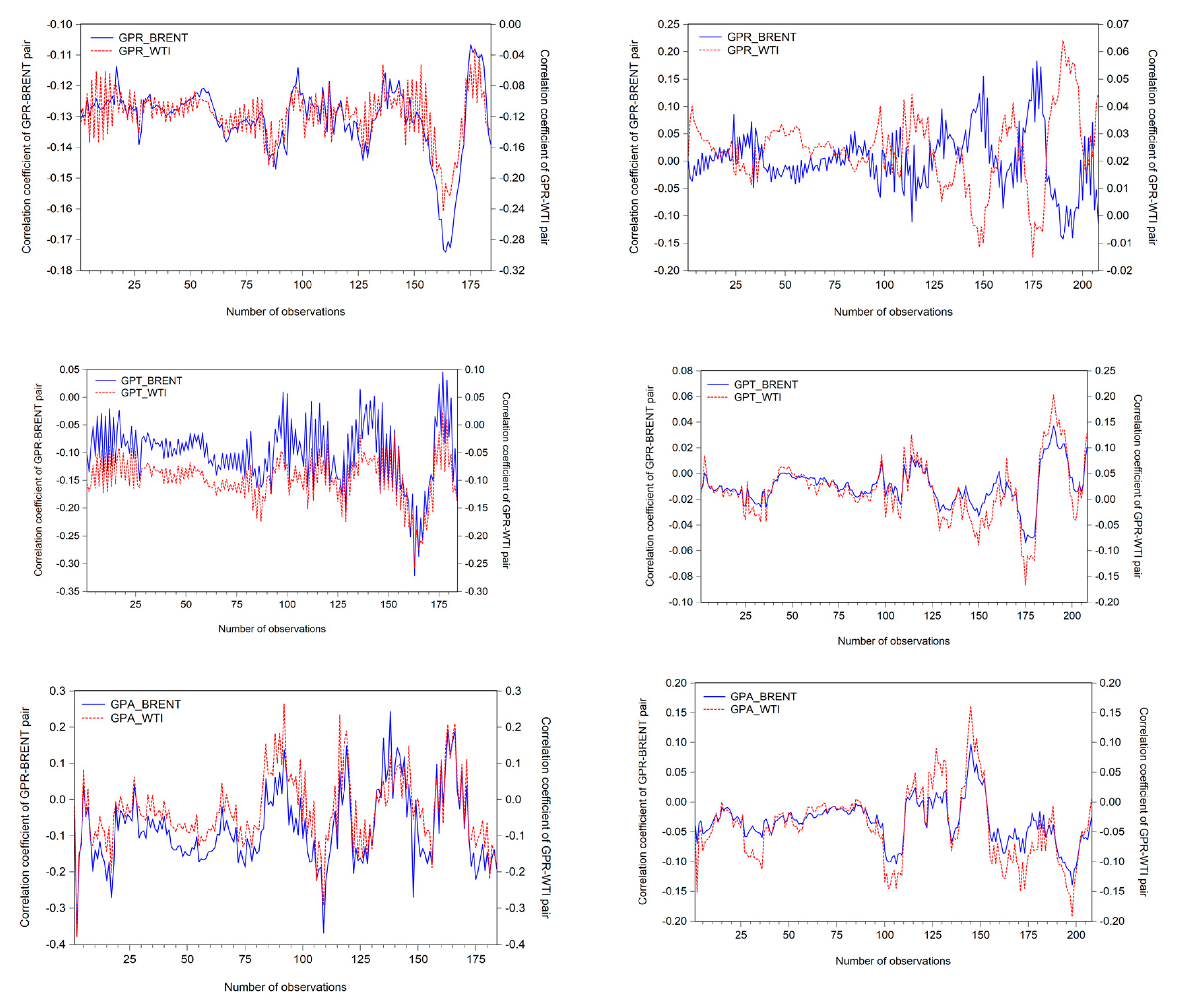
Geopolitical risks (related to potential risks or actual adverse events) and international crude oil prices may have a varying dynamic relationship in different political environments. Examining the heterogeneity of the dynamic correlation between geopolitical risks and international crude oil prices, geopolitical relations tend to be tense or moderate, which is beneficial to investors or policymakers in oil-producing countries to assess potential risks. Therefore, it is also an important contribution to analyze the dynamic correlation between geopolitical risk and international crude oil prices in different political environments. To test the heterogeneity of the dynamic correlation between geopolitical risk and international crude oil prices, we divided geopolitical relations into periods of tense and moderate tendencies based on the trend of the GPR index. Specifically, the observation that GPR index after the first-order difference is greater than 0 fell into the set “tense geopolitical relation period”, and less than 0 fell into the set “moderate geopolitical relation period”. Based on this, this study further estimated the dynamic correlation between geopolitical risks and crude oil prices under 184 sub-samples of tense geopolitical relation periods and 208 sub-samples of moderate geopolitical relation periods. Figure 6 presents the dynamic correlations between geopolitical risks and crude oil prices in different political environments.
The dynamic correlation between geopolitical risks and crude oil prices showed strong fluctuations during tense geopolitical relation periods. Figure 6 shows that, during tense geopolitical relation periods, the maximum value of the dynamic Kendall’s coefficient of the GPR-Brent pair was −0.107. By contrast, the maximum value of the dynamic Kendall’s coefficient of the GPR-WTI pair (GPT-Brent pair, GPT-WTI pair, GPA-Brent pair and GPA-WTI pair) was −0.033 (0.045, 0.023, 0.243 and 0.263, respectively). The minimum value of the dynamic Kendall’s coefficient of the GPR-Brent pair (GPR-WTI pair, GPT-Brent pair, GPT-WTI pair, GPA-Brent pair and GPA-WTI pair) was −0.174 (−0.243, −0.322, −0.257, −0.371 and −0.378, respectively). The amplitude of the dynamic Kendall’s coefficient of the GPR-Brent pair (GPR-WTI pair, GPT-Brent pair, GPT-WTI pair, GPA-Brent pair and GPA-WTI pair) was 0.068 (0.210, 0.367, 0.28, 0.614 and 0.641, respectively). However, during moderate geopolitical relation periods, the maximum value of the dynamic Kendall’s coefficient of the GPR-Brent pair was 0.183. By contrast, the maximum value of the dynamic Kendall’s coefficient of the GPR-WTI pair (GPT-Brent pair, GPT-WTI pair, GPA-Brent pair and GPA-WTI pair) was 0.064 (0.037, 0.203, 0.096 and 0.162, respectively). The minimum value of the dynamic Kendall’s coefficient of the GPR-Brent pair (GPR-WTI pair, GPT-Brent pair, GPT-WTI pair, GPA-Brent pair and GPA-WTI pair) was −0.142 (−0.015, −0.054, −0.167, −0.139 and −0.192, respectively). The amplitude of the dynamic Kendall’s coefficient of the GPR-Brent pair (GPR-WTI pair, GPT-Brent pair, GPT-WTI pair, GPA-Brent pair and GPA-WTI pair) was 0.325 (0.079, 0.091, 0.37, 0.235 and 0.354, respectively). Therefore, all dynamic Kendall’s coefficients of geopolitical relations and the crude oil prices, except the GPR-Brent pair and GPT-WTI pair, had a larger amplitude during tense geopolitical relation periods than during moderate geopolitical relation periods.
The standard deviation of the dynamic Kendall’s coefficients of geopolitical relation and crude oil prices can also draw the above conclusions. During tense geopolitical relation periods, the standard deviation of the dynamic Kendall’s coefficient of the GPR-Brent pair (GPR-WTI pair, GPT-Brent pair, GPT-WTI pair, GPA-Brent pair and GPA-WTI pair) was 0.011 (0.034, 0.057, 0.042, 0.104 and 0.097, respectively). By contrast, during moderate geopolitical relation periods, the standard deviation of the dynamic Kendall’s coefficient of the GPR-Brent pair (GPR-WTI pair, GPT-Brent pair, GPT-WTI pair, GPA-Brent pair and GPA-WTI pair) was 0.055 (0.013, 0.015, 0.056, 0.036 and 0.059, respectively). All dynamic Kendall’s coefficients of geopolitical relations and the crude oil prices, except the GPR-Brent pair and GPT-WTI pair, had a larger standard deviation during tense geopolitical relation periods than during moderate geopolitical relation periods.
In general, the correlation coefficient in periods of geopolitical tension had greater fluctuations than the correlation coefficient in periods of geopolitical moderation. This shows that the correlation between geopolitical risks and crude oil prices in different political environments is significantly different. In a tense political situation, the correlation between geopolitical risks and crude oil prices was more likely to change direction, and it is also prone to strong positive and strong negative correlations. In addition, the standard deviation of the dynamic correlation coefficient also reflects the same fact—the dynamic correlation between geopolitical risks and crude oil prices showed strong fluctuations during tense geopolitical relation periods.
4.2. Granger Causality Test
From the above empirical results, it can be concluded that geopolitical factors have a significant correlation with international crude oil prices. However, this cannot infer a causal relationship between geopolitical factors and international crude oil prices. To reveal a causal linkage between geopolitical factors and crude oil prices, this study implemented the Granger causality tests to test whether there is a causal relationship between geopolitical factors and crude oil prices. The causality tests were implemented for the GPR index, GPT index, GPA index, Brent and WTI. In this study, the Granger causality tests were implemented within a first-order to sixth-order lag. The results of the Granger causality with first-order lag are shown in Table 3.
For the full sample period, there was unidirectional Granger causality running from geopolitical factors to crude oil prices. Table 3 shows that during the full sample period, the GPR index was the unidirectional Granger causality of Brent and WTI, with a 5% significance level. In addition, the GPT index was the unidirectional Granger causality of Brent and WTI, with 5% and 10% significance levels, respectively. However, there was no Granger causality between the GPA index and crude oil prices. This shows that during the full sample period, geopolitical risks and geopolitical threats can directly cause fluctuations in international crude oil prices. By contrast, the correlation between geopolitical actions and crude oil prices may be facilitated by a third factor. In addition, research presented by Wen et al. [56] showed that oil prices and stock markets have non-linear causal crossings. The reason may be that fluctuations in the financial market have led to rising oil prices. Our results also showed that, in the sub-sample period, there was no Granger causality between geopolitical factors and crude oil prices, whether during tense geopolitical relation periods or moderate geopolitical relation periods.
However, it can be seen from Table 4 that only Brent was a unidirectional Granger causality of GPT during the full sample period. Specifically, at a 10% significance level and a 2-month lag, there was unidirectional Granger causality running from Brent to GPT. By contrast, the null hypotheses “Crude oil prices do not Granger cause geopolitical factors” or “Geopolitical factors do not Granger cause crude oil prices” cannot be rejected. Such a result of Granger causality occurred simultaneously in the full sample period, tense geopolitical relation periods, and moderate geopolitical relation periods. In addition, the Granger causality tests within third-order to sixth-order lags were not significant. Therefore, we do not show these results in the text.
5. Conclusions and Policy Recommendations
In this paper, we examined the dynamic correlations between geopolitical factors and crude oil prices from June 1987 to February 2020. We utilized the time-varying copula approach to study the dynamic correlation between the GPR index (GPT index and GPA index) constructed by Caldara and Iacoviello [5] and crude oil prices. We also examined the heterogeneity of the dynamic correlation between geopolitical factors and crude oil prices during periods of tense and moderate geopolitical relations. Subsequently, we employed the Granger Causality tests to reveal a causal linkage between geopolitical factors and crude oil prices.
This study contributes to the literatures on the relationship between geopolitical factors and crude oil prices, which can be summarized as follows:
First, the correlations between geopolitical factors and crude oil prices were greater when extreme political events happened. After the Gulf War, the correlation between the GPR index and crude oil prices attained its minimum value during the period 1990–2000, showing a strongly negative correlation. With the frequent occurrence of extreme political events in the early 21st century (for example, the 9/11 event and Iraq invasion). Second, the dynamic correlation coefficient of the GPA and crude oil prices was not always negative. The results found by examining the dynamic correlations between the sub-indices and crude oil prices suggested that the dynamic correlation between the GPT index and crude oil prices was negatively correlated in all samples. However, the dynamic correlation between the GPA index and crude oil prices met a positive value during the period when extreme political events happened. This means that GPA and crude oil prices were positively correlated during this period. Third, the dynamic correlation between geopolitical factors and crude oil prices showed strong volatility during periods of political tension. All coefficients of dynamic correlation between geopolitical factors and the crude oil prices, except the GPR-Brent pair and GPT-WTI pair, had larger amplitudes during periods of political tension. Besides, all dynamic correlation coefficients, except the GPR-Brent pair and GPT-WTI pair, also had larger standard deviations during periods of political tension. The results also revealed that there was unidirectional Granger causality running from geopolitical factors to crude oil prices in the full sample period.
The political implications of these findings are that (1) the level of attention to traditional oil exporting countries needs to be strengthened. In the future, the Middle East will remain the world’s main oil exporting region. According to the “World Energy Outlook 2035” released by British Petroleum (BP), the oil production of OPEC (organization of the petroleum exporting countries) countries in the Middle East will increase by 7 million barrels per day by 2035. The stability of the geopolitical situation in this region will directly affect the trend of international oil; (2) the serious challenges posed by international terrorism to international oil prices require close attention. As far as the current situation is concerned, terrorist attacks will not significantly change the general direction of the global oil market. However, as terrorism spread globally, the fluctuations in international oil prices caused by terrorist incidents have become more apparent. At the same time, the occurrence of terrorist incidents will lead to an increase in global risk sentiment, which will surely cause panic in the global investment field.
This study opens new avenues for future research. As a first extension, further research may examine the risk spillover from geopolitical factors to crude oil prices, such as the empirical framework of Liu et al. [57]. As a second extension, future research could detect the mediating variables or the moderating variables in the correlation between geopolitical factors and crude oil prices.
Author Contributions
Conceptualization, F.L. and J.Z.; methodology, F.L. and J.Z.; software, J.Z.; formal analysis, J.Z.; resources, F.L.; writing—original draft preparation, F.L., Z.H. and J.Z.; writing—review and editing, Z.H., J.Z. and K.A.; supervision, F.L. and J.Z.; project administration, F.L. All authors have read and agreed to the published version of the manuscript.
Funding
This research received no external funding.
Conflicts of Interest
The authors declare no conflict of interest.
Appendix A

Table A1.
Nomenclatures.
| Abbreviation | Full Name |
|---|---|
| GPR | Geopolitical Risk |
| GPT | Geopolitical Threats |
| GPA | Geopolitical Acts |
| WTI | West Texas Intermediate |
| OPEC | Organization of the Petroleum Exporting Countries |
| ARCH | Autoregressive Conditional Heteroscedasticity |
| GARCH | Generalized Autoregressive Conditional Heteroscedasticity |
| AR | Autoregressive |
| MA | Moving Average |
| ARMA | Autoregressive Moving Average |
| ARIMA | Autoregressive Integrated Moving Average |
| AIC | Akaike Information Criteria |
| ML | Maximum Likelihood |
References
- Salameh, M.G. Where Is the Crude Oil Price Headed? 2014. Available online: http://dx.doi.org/10.2139/ssrn.2502056 (accessed on 28 March 2020).
- Azzimonti, M. Partisan conflict and private investment. J. Monet. Econ. 2018, 93, 114–131. [Google Scholar] [CrossRef] [Green Version]
- Monge, M.; Gil-Alana, L.A.; de Gracia, F.P. Crude oil price behaviour before and after military conflicts and geopolitical events. Energy 2017, 120, 79–91. [Google Scholar] [CrossRef]
- Liao, G.; Li, Z.; Du, Z.; Liu, Y. The heterogeneous interconnections between supply or demand side and oil risks. Energies 2019, 12, 2226. [Google Scholar] [CrossRef] [Green Version]
- Caldara, D.; Iacoviello, M. Measuring geopolitical risk. In International Finance Discussion Paper; FRB: Washington, DC, USA, 2018. [Google Scholar]
- Zhang, X.; Yu, L.; Wang, S.; Lai, K.K. Estimating the impact of extreme events on crude oil price: An EMD-based event analysis method. Energy Econ. 2009, 31, 768–778. [Google Scholar] [CrossRef]
- Dey, A.K.; Edwards, A.; Das, K.P. Determinants of High Crude Oil Price: A Nonstationary Extreme Value Approach. J. Stat. Theory Pract. 2020, 14, 4. [Google Scholar] [CrossRef]
- Ji, Q.; Liu, B.-Y.; Nehler, H.; Uddin, G.S. Uncertainties and extreme risk spillover in the energy markets: A time-varying copula-based CoVaR approach. Energy Econ. 2018, 76, 115–126. [Google Scholar] [CrossRef]
- Bilgin, M.H.; Gozgor, G.; Karabulut, G. The impact of world energy price volatility on aggregate economic activity in developing Asian economies. Singap. Econ. Rev. 2015, 60, 1550009. [Google Scholar] [CrossRef]
- Bildirici, M.E.; Badur, M.M. The effects of oil prices on confidence and stock return in China, India and Russia. Quant. Financ. Econ. 2018, 2, 884–903. [Google Scholar] [CrossRef]
- Li, Z.; Zhong, J. Impact of economic policy uncertainty shocks on China’s financial conditions. Financ. Res. Lett. 2019, 35, 101303. [Google Scholar] [CrossRef]
- Rasoulinezhad, E.; Taghizadeh-Hesary, F.; Sung, J.; Panthamit, N. Geopolitical risk and energy transition in russia: Evidence from ARDL bounds testing method. Sustainability 2020, 12, 2689. [Google Scholar] [CrossRef] [Green Version]
- Taghizadeh-Hesary, F.; Yoshino, N.; Mohammadi Hossein Abadi, M.; Farboudmanesh, R. Response of macro variables of emerging and developed oil importers to oil price movements. J. Asia Pac. Econ. 2016, 21, 91–102. [Google Scholar] [CrossRef] [Green Version]
- Gaibulloev, K.; Sandler, T. Growth consequences of terrorism in Western Europe. Kyklos 2008, 61, 411–424. [Google Scholar] [CrossRef] [Green Version]
- Ji, Q.; Li, J.; Sun, X. Measuring the interdependence between investor sentiment and crude oil returns: New evidence from the CFTC’s disaggregated reports. Financ. Res. Lett. 2019, 30, 420–425. [Google Scholar] [CrossRef]
- Noguera-Santaella, J. Geopolitics and the oil price. Econ. Model. 2016, 52, 301–309. [Google Scholar] [CrossRef]
- Liu, Y.; Dong, H.; Failler, P. The oil market reactions to OPEC’s announcements. Energies 2019, 12, 3238. [Google Scholar] [CrossRef] [Green Version]
- Li, Z.; Dong, H.; Huang, Z.; Failler, P. Asymmetric effects on risks of Virtual Financial Assets (VFAs) in different regimes: A Case of Bitcoin. Quant. Financ. Econ. 2018, 2, 860–883. [Google Scholar] [CrossRef]
- Balcilar, M.; Bonato, M.; Demirer, R.; Gupta, R. Geopolitical risks and stock market dynamics of the BRICS. Econ. Syst. 2018, 42, 295–306. [Google Scholar] [CrossRef] [Green Version]
- Antonakakis, N.; Gupta, R.; Kollias, C.; Papadamou, S. Geopolitical risks and the oil-stock nexus over 1899–2016. Financ. Res. Lett. 2017, 23, 165–173. [Google Scholar] [CrossRef] [Green Version]
- Aysan, A.F.; Demir, E.; Gozgor, G.; Lau, C.K.M. Effects of the geopolitical risks on Bitcoin returns and volatility. Res. Int. Bus. Financ. 2019, 47, 511–518. [Google Scholar] [CrossRef] [Green Version]
- Cunado, J.; Gupta, R.; Lau, C.K.M.; Sheng, X. Time-varying impact of geopolitical risks on oil prices. Def. Peace Econ. 2019, 1–15. [Google Scholar] [CrossRef]
- Bilgin, M.H.; Gozgor, G.; Karabulut, G. How Do Geopolitical Risks Affect Government Investment? An Empirical Investigation. Def. Peace Econ. 2018, 1–15. [Google Scholar] [CrossRef]
- Gupta, R.; Gozgor, G.; Kaya, H.; Demir, E. Effects of geopolitical risks on trade flows: Evidence from the gravity model. Eurasian Econ. Rev. 2019, 9, 515–530. [Google Scholar] [CrossRef]
- Demiralay, S.; Kilincarslan, E. The impact of geopolitical risks on travel and leisure stocks. Tour. Manag. 2019, 75, 460–476. [Google Scholar] [CrossRef]
- Mei, D.; Ma, F.; Liao, Y.; Wang, L. Geopolitical risk uncertainty and oil future volatility: Evidence from MIDAS models. Energy Econ. 2020, 86, 104624. [Google Scholar] [CrossRef]
- Benhmad, F. Modeling nonlinear Granger causality between the oil price and US dollar: A wavelet based approach. Econ. Model. 2012, 29, 1505–1514. [Google Scholar] [CrossRef]
- Zhong, J.; Wang, M.; Drakeford, B.; Li, T. Spillover effects between oil and natural gas prices: Evidence from emerging and developed markets. Green Financ. 2019, 1, 30–45. [Google Scholar] [CrossRef]
- Wolfe, M.H.; Rosenman, R. Bidirectional causality in oil and gas markets. Energy Econ. 2014, 42, 325–331. [Google Scholar] [CrossRef]
- Lee, C.-C.; Chiu, Y.-B. Nuclear energy consumption, oil prices, and economic growth: Evidence from highly industrialized countries. Energy Econ. 2011, 33, 236–248. [Google Scholar] [CrossRef]
- Cooke, B. Recent Food Prices Movements: A Time Series Analysis; Internationl Food Policy Research Institute: Washington, DC, USA, 2009; Volume 942. [Google Scholar]
- Bildirici, M.E.; Turkmen, C. Nonlinear causality between oil and precious metals. Resour. Policy 2015, 46, 202–211. [Google Scholar] [CrossRef]
- Brini, R.; Amara, M.; Jemmali, H. Renewable energy consumption, International trade, oil price and economic growth inter-linkages: The case of Tunisia. Renew. Sustain. Energy Rev. 2017, 76, 620–627. [Google Scholar] [CrossRef]
- Wen, F.; Min, F.; Zhang, Y.J.; Yang, C. Crude oil price shocks, monetary policy, and China’s economy. Int. J. Financ. Econ. 2019, 24, 812–827. [Google Scholar] [CrossRef]
- Ouyang, S.; Dong, H. Oil price pass-through into consumer and producer prices with monetary policy in China: Are there non-linear and mediating effects. Front. Energy Res. 2020, 8, 35. [Google Scholar]
- Dong, H.; Liu, Y.; Chang, J. The heterogeneous linkage of economic policy uncertainty and oil return risks. Green Financ. 2019, 1, 46–66. [Google Scholar] [CrossRef]
- Li, Z.; Liao, G.; Albitar, K. Does corporate environmental responsibility engagement affect firm value? The mediating role of corporate innovation. Bus. Strategy Environ. 2020, 29, 1045–1055. [Google Scholar] [CrossRef]
- Bal, D.P.; Rath, B.N. Nonlinear causality between crude oil price and exchange rate: A comparative study of China and India. Energy Econ. 2015, 51, 149–156. [Google Scholar]
- Su, C.-W.; Khan, K.; Tao, R.; Nicoleta-Claudia, M. Does geopolitical risk strengthen or depress oil prices and financial liquidity? Evidence from Saudi Arabia. Energy 2019, 187, 116003. [Google Scholar] [CrossRef]
- Ji, Q.; Liu, B.-Y.; Fan, Y. Risk dependence of CoVaR and structural change between oil prices and exchange rates: A time-varying copula model. Energy Econ. 2019, 77, 80–92. [Google Scholar] [CrossRef]
- Li, T.; Zhong, J.; Huang, Z. Potential dependence of financial cycles between emerging and developed countries: Based on ARIMA-GARCH Copula model. Emerg. Mark. Financ. Trade 2019, 1–14. [Google Scholar] [CrossRef]
- Hemche, O.; Jawadi, F.; Maliki, S.B.; Cheffou, A.I. On the study of contagion in the context of the subprime crisis: A dynamic conditional correlation–multivariate GARCH approach. Econ. Model. 2016, 52, 292–299. [Google Scholar] [CrossRef]
- Sklar, A.; Sklar, A.; Sklar, C. Fonctions De Reprtition an Dimensions Et Leursmarges; de l’Institut Statistique de l’Université de Paris: Paris, France, 1959. [Google Scholar]
- Patton, A.J. Modelling asymmetric exchange rate dependence. Int. Econ. Rev. 2006, 47, 527–556. [Google Scholar] [CrossRef]
- Charles, A.; Darné, O. Forecasting crude-oil market volatility: Further evidence with jumps. Energy Econ. 2017, 67, 508–519. [Google Scholar] [CrossRef]
- Scheitrum, D.P.; Carter, C.A.; Revoredo-Giha, C. WTI and Brent futures pricing structure. Energy Econ. 2018, 72, 462–469. [Google Scholar] [CrossRef]
- Klein, T. Trends and contagion in WTI and Brent crude oil spot and futures markets-The role of OPEC in the last decade. Energy Econ. 2018, 75, 636–646. [Google Scholar] [CrossRef] [Green Version]
- Bai, X.; Lam, J.S.L. A copula-GARCH approach for analyzing dynamic conditional dependency structure between liquefied petroleum gas freight rate, product price arbitrage and crude oil price. Energy Econ. 2019, 78, 412–427. [Google Scholar] [CrossRef]
- Sahamkhadam, M.; Stephan, A.; Östermark, R. Portfolio optimization based on GARCH-EVT-Copula forecasting models. Int. J. Forecast. 2018, 34, 497–506. [Google Scholar] [CrossRef]
- Baker, S.R.; Bloom, N.; Davis, S.J. Measuring economic policy uncertainty. Q. J. Econ. 2016, 131, 1593–1636. [Google Scholar] [CrossRef]
- Huang, Y.; Luk, P. Measuring economic policy uncertainty in China. China Econ. Rev. 2020, 59, 101367. [Google Scholar] [CrossRef]
- Plourde, A.; Watkins, G.C. Crude oil prices between 1985 and 1994: How volatile in relation to other commodities? Resour. Energy Econ. 1998, 20, 245–262. [Google Scholar] [CrossRef]
- Zhang, Y.-J. Speculative trading and WTI crude oil futures price movement: An empirical analysis. Appl. Energy 2013, 107, 394–402. [Google Scholar] [CrossRef]
- Coleman, L. Explaining crude oil prices using fundamental measures. Energy Policy 2012, 40, 318–324. [Google Scholar] [CrossRef]
- Caldara, D.; Cavallo, M.; Iacoviello, M. Oil price elasticities and oil price fluctuations. J. Monet. Econ. 2019, 103, 1–20. [Google Scholar] [CrossRef] [Green Version]
- Wen, F.; Xiao, J.; Xia, X.; Chen, B.; Xiao, Z.; Li, J. Oil prices and chinese stock market: Nonlinear causality and volatility persistence. Emerg. Mark. Financ. Trade 2019, 55, 1247–1263. [Google Scholar] [CrossRef]
- Liu, K.; Luo, C.; Li, Z. Investigating the risk spillover from crude oil market to BRICS stock markets based on Copula-POT-CoVaR models. Quant. Financ. Econ. 2019, 3, 754. [Google Scholar] [CrossRef]
Figure 1.
Monthly GPR indices and crude oil prices. Note: GPR, GPT, GPA, BRENT, and WTI represent geopolitical risk index, geopolitical threats index, geopolitical acts index, Brent, and WTI spot prices, respectively. The sample period is from June 1987 to February 2020.
Figure 1.
Monthly GPR indices and crude oil prices. Note: GPR, GPT, GPA, BRENT, and WTI represent geopolitical risk index, geopolitical threats index, geopolitical acts index, Brent, and WTI spot prices, respectively. The sample period is from June 1987 to February 2020.

Figure 2.
Dynamic correlations between the GPR index and crude oil prices. Note: GPR_BRENT and GPR_WTI represent the dynamic Kendall’s coefficients of the GPR-Brent pair and GPR-WTI pair, respectively. The sample period is from June 1987 to February 2020.
Figure 2.
Dynamic correlations between the GPR index and crude oil prices. Note: GPR_BRENT and GPR_WTI represent the dynamic Kendall’s coefficients of the GPR-Brent pair and GPR-WTI pair, respectively. The sample period is from June 1987 to February 2020.

Figure 3.
Dynamic conditional correlations (DCC) between the GPR index and crude oil prices. Note: GPR_BRENT and GPR_WTI represent the dynamic conditional correlations of the GPR-Brent pair and GPR-WTI pair, respectively. The sample period is from June 1987 to February 2020.
Figure 3.
Dynamic conditional correlations (DCC) between the GPR index and crude oil prices. Note: GPR_BRENT and GPR_WTI represent the dynamic conditional correlations of the GPR-Brent pair and GPR-WTI pair, respectively. The sample period is from June 1987 to February 2020.

Figure 4.
Wavelet coherence between the GPR index and crude oil prices. Note: the left sub-plot and the right sub-plot represent wavelet coherence of the GPR-Brent pair and GPR-WTI pair, respectively. The sample period is from June 1987 to February 2020.
Figure 4.
Wavelet coherence between the GPR index and crude oil prices. Note: the left sub-plot and the right sub-plot represent wavelet coherence of the GPR-Brent pair and GPR-WTI pair, respectively. The sample period is from June 1987 to February 2020.

Figure 5.
Dynamic correlations between the GPT/GPA indexes and crude oil prices. Note: the upper sub-figure presents the dynamic Kendall’s coefficients of the GPT-Brent pair and GPT-WTI pair. The lower sub-figure presents the dynamic Kendall’s coefficients of the GPA-Brent pair and GPA-WTI pair. GPT-BRENT, GPT-WTI, GPA-BRENT and GPA-WTI represent the dynamic Kendall’s coefficients of GPT-Brent pair, GPT-WTI pair, GPA-Brent pair and GPA-WTI pair, respectively. The sample period is from June 1987 to February 2020.


Figure 6.
Dynamic correlations between geopolitical risks and crude oil prices in different political environments. Note: the sub-figure on the left presents the dynamic Kendall’s coefficients of the GPR-Brent pair, GPR-WTI pair, GPT-Brent pair, GPT-WTI pair, GPA-Brent pair and GPA-WTI pair during tense geopolitical relation periods. The sub-figure on the right presents the dynamic Kendall’s coefficients during moderate geopolitical relation periods. GPR-BRENT, GPR-WTI, GPT-BRENT, GPT-WTI, GPA-BRENT and GPA-WTI represent the dynamic Kendall’s coefficients of the GPR-Brent pair, GPR-WTI pair, GPT-Brent pair, GPT-WTI pair, GPA-Brent pair and GPA-WTI pair, respectively. The sample period is from June 1987 to February 2020.

Table 1.
Descriptive statistics.
| Variable | Mean | Max. | Min. | Std. Dev. | Skew. | Kurt. | Obs. |
|---|---|---|---|---|---|---|---|
| Overall | |||||||
| GPR | 85.849 | 545.09 | 23.7 | 65.334 | 2.951 | 15.924 | 393 |
| GPT | 88.421 | 602.45 | 20.23 | 72.044 | 2.971 | 16.167 | 393 |
| GPA | 72.689 | 496.89 | 11.09 | 59.074 | 3.869 | 23.122 | 393 |
| BRENT | 46.666 | 132.72 | 9.82 | 32.643 | 0.858 | 2.532 | 393 |
| WTI | 45.444 | 133.88 | 11.35 | 29.094 | 0.813 | 2.539 | 393 |
| Tension | |||||||
| GPR | 100.782 | 545.090 | 26.920 | 80.705 | 2.657 | 12.032 | 184 |
| GPT | 105.231 | 602.450 | 24.320 | 89.582 | 2.630 | 11.937 | 184 |
| GPA | 79.202 | 496.890 | 11.090 | 65.469 | 3.591 | 19.892 | 184 |
| BRENT | 48.130 | 132.720 | 9.820 | 34.239 | 0.808 | 2.362 | 184 |
| WTI | 46.713 | 133.880 | 11.350 | 30.413 | 0.784 | 2.463 | 184 |
| Stabilization | |||||||
| GPR | 72.641 | 268.580 | 23.700 | 44.178 | 1.674 | 6.199 | 208 |
| GPT | 73.564 | 290.040 | 20.230 | 47.556 | 1.642 | 5.892 | 208 |
| GPA | 66.871 | 473.730 | 13.270 | 52.412 | 4.136 | 26.599 | 208 |
| BRENT | 45.505 | 123.260 | 11.110 | 31.217 | 0.882 | 2.654 | 208 |
| WTI | 44.443 | 125.400 | 12.520 | 27.924 | 0.817 | 2.547 | 208 |
Note: The overall panel summarizes the descriptive statistics for the full sample. The tension panel is for the periods of geopolitical tension, and the stabilization panel is for the periods of geopolitical stabilization. ‘Max.’, ‘Min.’, ‘Std. Dev.’, ‘Skew.’, ‘Kurt.’, and ‘Obs.’ represent maximum, minimum, standard deviation, skewness, kurtosis, and observation, respectively. GPR, GPT, GPA, BRENT, and WTI represent geopolitical risk index, geopolitical threats index, geopolitical acts index, Brent, and WTI spot prices, respectively. For detailed rules on the division of periods of geopolitical tension and stabilization, please refer to Section 4.1 of this paper. The sample period is from June 1987 to February 2020.
Table 2.
Parameter estimation of the ARIMA-GARCH models for GPR indices and crude oil prices.
| Variable | GPR | GPT | GPA | BRENT | WTI |
|---|---|---|---|---|---|
| −0.835 *** (0.263) | −0.85 *** (0.272) | −0.539 *** (0.084) | 0.003 (0.066) | 0.039 (0.12) | |
| 0.057 (0.198) | −0.012 (0.181) | 0.599 *** (0.037) | 0.906 *** (0.067) | −0.162 (1.282) | |
| −0.509 *** (0.191) | −0.449 *** (0.173) | −1.17 *** (0.001) | −0.664 *** (0.084) | 0.416 (1.28) | |
| −0.212 * (0.122) | −0.247 ** (0.108) | 0.191 *** (0.001) | −0.272 *** (0.058) | 0.059 (0.319) | |
| 117.495 ** (49.876) | 106.206 ** (49.272) | 1057.199 ** (470.339) | 0.144 * (0.085) | 0.114 * (0.069) | |
| 0.45 *** (0.13) | 0.414 *** (0.12) | 0.639 * (0.357) | 0.253 *** (0.05) | 0.194 *** (0.039) | |
| 0.549 *** (0.113) | 0.585 *** (0.112) | 0.106 (0.117) | 0.746 *** (0.047) | 0.805 *** (0.035) | |
| shape | 2.98 *** (0.32) | 3.008 *** (0.323) | 2.558 *** (0.333) | 12.206 ** (5.089) | 8.806 *** (2.86) |
Notes: ARIMA-GARCH represent autoregressive integrated moving average-generalized autoregressive conditional heteroscedasticity model. GPR, GPT, GPA, BRENT, and WTI represent geopolitical risk index, geopolitical threats index, geopolitical acts index, Brent, and WTI spot prices, respectively. The standard errors of the parameters are in parenthesis. *, **, and *** represent 10%, 5% and 1% significance, respectively. The sample period is from June 1987 to February 2020.
Table 3.
Results of Granger causality test with first-order lag.
| Null Hypothesis: | Obs. | Lag (month) | F-Statistic | Prob. | Sign. |
|---|---|---|---|---|---|
| BRENT ⇏ GPR | 392 | 1 | 1.313 | 0.2526 | Cannot reject |
| GPR ⇏ BRENT | 1 | 4.33847 | 0.0379 | Reject | |
| WTI ⇏ GPR | 392 | 1 | 1.21456 | 0.2711 | Cannot reject |
| GPR ⇏ WTI | 1 | 3.94318 | 0.0478 | Reject | |
| BRENT ⇏ GPT | 392 | 1 | 1.63395 | 0.2019 | Cannot reject |
| GPT ⇏ BRENT | 1 | 4.17903 | 0.0416 | Reject | |
| WTI ⇏ GPT | 392 | 1 | 1.4533 | 0.2287 | Cannot reject |
| GPT ⇏ WTI | 1 | 3.71016 | 0.0548 | Reject | |
| BRENT ⇏ GPA | 392 | 1 | 0.22511 | 0.6354 | Cannot reject |
| GPA ⇏ BRENT | 1 | 2.45973 | 0.1176 | Cannot reject | |
| WTI ⇏ GPA | 392 | 1 | 0.09376 | 0.7596 | Cannot reject |
| GPA ⇏ WTI | 1 | 2.63677 | 0.1052 | Cannot reject | |
| BRENT ⇏ GPR | 183 | 1 | 0.77072 | 0.3812 | Cannot reject |
| GPR ⇏ BRENT | 1 | 0.99295 | 0.3204 | Cannot reject | |
| WTI ⇏ GPR | 183 | 1 | 0.56853 | 0.4518 | Cannot reject |
| GPR ⇏ WTI | 1 | 1.14897 | 0.2852 | Cannot reject | |
| BRENT ⇏ GPT | 183 | 1 | 0.84317 | 0.3597 | Cannot reject |
| GPT ⇏ BRENT | 1 | 1.08404 | 0.2992 | Cannot reject | |
| WTI ⇏ GPT | 183 | 1 | 0.59835 | 0.4402 | Cannot reject |
| GPT ⇏ WTI | 1 | 1.25532 | 0.264 | Cannot reject | |
| BRENT ⇏ GPA | 183 | 1 | 0.2487 | 0.6186 | Cannot reject |
| GPA ⇏ BRENT | 1 | 0.12509 | 0.724 | Cannot reject | |
| WTI ⇏ GPA | 183 | 1 | 0.15276 | 0.6964 | Cannot reject |
| GPA ⇏ WTI | 1 | 0.14529 | 0.7035 | Cannot reject | |
| BRENT ⇏ GPR | 207 | 1 | 0.94348 | 0.3325 | Cannot reject |
| GPR ⇏ BRENT | 1 | 0.54775 | 0.4601 | Cannot reject | |
| WTI ⇏ GPR | 207 | 1 | 0.93918 | 0.3336 | Cannot reject |
| GPR ⇏ WTI | 1 | 0.3836 | 0.5364 | Cannot reject | |
| BRENT ⇏ GPT | 207 | 1 | 1.12381 | 0.2904 | Cannot reject |
| GPT ⇏ BRENT | 1 | 0.82501 | 0.3648 | Cannot reject | |
| WTI ⇏ GPT | 207 | 1 | 1.10528 | 0.2944 | Cannot reject |
| GPT ⇏ WTI | 1 | 0.63606 | 0.4261 | Cannot reject | |
| BRENT ⇏ GPA | 207 | 1 | 0.27616 | 0.5998 | Cannot reject |
| GPA ⇏ BRENT | 1 | 0.0806 | 0.7768 | Cannot reject | |
| WTI ⇏ GPA | 207 | 1 | 0.18129 | 0.6707 | Cannot reject |
| GPA ⇏ WTI | 1 | 0.16424 | 0.6857 | Cannot reject |
Note: This table summarizes the results of the first-order lag Granger causality test for geopolitical risk indices (GPR, GPT and GPA) and crude oil prices (BRENT and WTI). Obs., Prob., and Sign. represent Observation, Probability, and Significance, respectively. The observations of 392, 183 and 207 represent the full sample period, tense geopolitical relation period, and moderate geopolitical relation period, respectively.
Table 4.
Results of Granger causality test with first-order lag.
| Null Hypothesis: | Obs. | Lag (month) | F-Statistic | Prob. | Sign. |
|---|---|---|---|---|---|
| BRENT ⇏ GPR | 391 | 2 | 2.29025 | 0.1026 | Cannot reject |
| GPR ⇏ BRENT | 2 | 1.43025 | 0.2405 | Cannot reject | |
| WTI ⇏ GPR | 391 | 2 | 1.86755 | 0.1559 | Cannot reject |
| GPR ⇏ WTI | 2 | 1.39884 | 0.2481 | Cannot reject | |
| BRENT ⇏ GPT | 391 | 2 | 2.57553 | 0.0774 | Reject |
| GPT ⇏ BRENT | 2 | 1.36463 | 0.2567 | Cannot reject | |
| WTI ⇏ GPT | 391 | 2 | 1.98638 | 0.1386 | Cannot reject |
| GPT ⇏ WTI | 2 | 1.31018 | 0.2710 | Cannot reject | |
| BRENT ⇏ GPA | 391 | 2 | 0.32557 | 0.7223 | Cannot reject |
| GPA ⇏ BRENT | 2 | 0.98266 | 0.3752 | Cannot reject | |
| WTI ⇏ GPA | 391 | 2 | 0.32404 | 0.7234 | Cannot reject |
| GPA ⇏ WTI | 2 | 1.48253 | 0.2284 | Cannot reject | |
| BRENT ⇏ GPR | 182 | 2 | 1.87035 | 0.1571 | Cannot reject |
| GPR ⇏ BRENT | 2 | 0.47908 | 0.6202 | Cannot reject | |
| WTI ⇏ GPR | 182 | 2 | 1.27094 | 0.2831 | Cannot reject |
| GPR ⇏ WTI | 2 | 0.60043 | 0.5497 | Cannot reject | |
| BRENT ⇏ GPT | 182 | 2 | 1.78862 | 0.1702 | Cannot reject |
| GPT ⇏ BRENT | 2 | 0.60359 | 0.5480 | Cannot reject | |
| WTI ⇏ GPT | 182 | 2 | 1.17516 | 0.3112 | Cannot reject |
| GPT ⇏ WTI | 2 | 0.74320 | 0.4771 | Cannot reject | |
| BRENT ⇏ GPA | 182 | 2 | 0.95770 | 0.3858 | Cannot reject |
| GPA ⇏ BRENT | 2 | 0.28308 | 0.7538 | Cannot reject | |
| WTI ⇏ GPA | 182 | 2 | 0.67582 | 0.5100 | Cannot reject |
| GPA ⇏ WTI | 2 | 0.19757 | 0.8209 | Cannot reject | |
| BRENT ⇏ GPR | 206 | 2 | 1.05852 | 0.3489 | Cannot reject |
| GPR ⇏ BRENT | 2 | 1.61006 | 0.2024 | Cannot reject | |
| WTI ⇏ GPR | 206 | 2 | 1.00058 | 0.3695 | Cannot reject |
| GPR ⇏ WTI | 2 | 1.11911 | 0.3286 | Cannot reject | |
| BRENT ⇏ GPT | 206 | 2 | 1.04075 | 0.3551 | Cannot reject |
| GPT ⇏ BRENT | 2 | 1.81407 | 0.1656 | Cannot reject | |
| WTI ⇏ GPT | 206 | 2 | 1.13876 | 0.3223 | Cannot reject |
| GPT ⇏ WTI | 2 | 1.29969 | 0.2749 | Cannot reject | |
| BRENT ⇏ GPA | 206 | 2 | 0.32544 | 0.7226 | Cannot reject |
| GPA ⇏ BRENT | 2 | 0.39268 | 0.6758 | Cannot reject | |
| WTI ⇏ GPA | 206 | 2 | 0.10420 | 0.9011 | Cannot reject |
| GPA ⇏ WTI | 2 | 0.43008 | 0.6511 | Cannot reject |
Note: This table summarizes the results of the first-order lag Granger causality test for geopolitical risk indices (GPR, GPT and GPA) and crude oil prices (BRENT and WTI). Obs., Prob., and Sign. represent Observation, Probability, and Significance, respectively. The observations of 391, 182 and 206 represent the full sample period, tense geopolitical relation periods, and moderate geopolitical relation periods, respectively.
© 2020 by the authors. Licensee MDPI, Basel, Switzerland. This article is an open access article distributed under the terms and conditions of the Creative Commons Attribution (CC BY) license (http://creativecommons.org/licenses/by/4.0/).
Share and Cite
MDPI and ACS Style
Li, F.; Huang, Z.; Zhong, J.; Albitar, K. Do Tense Geopolitical Factors Drive Crude Oil Prices? Energies 2020, 13, 4277. https://doi.org/10.3390/en13164277
AMA Style
Li F, Huang Z, Zhong J, Albitar K. Do Tense Geopolitical Factors Drive Crude Oil Prices? Energies. 2020; 13(16):4277. https://doi.org/10.3390/en13164277
Chicago/Turabian StyleLi, Fen, Zhehao Huang, Junhao Zhong, and Khaldoon Albitar. 2020. "Do Tense Geopolitical Factors Drive Crude Oil Prices?" Energies 13, no. 16: 4277. https://doi.org/10.3390/en13164277
Note that from the first issue of 2016, this journal uses article numbers instead of page numbers. See further details here.