Developing Induction Motor State Observers with Increased Robustness


Faculty of Electrical Engineering, Silesian University of Technology, 44-100 Gliwice, Poland
*
Author to whom correspondence should be addressed.
Energies 2020, 13(20), 5487; https://doi.org/10.3390/en13205487
Submission received: 28 September 2020
/
Revised: 11 October 2020
/
Accepted: 14 October 2020
/
Published: 20 October 2020
(This article belongs to the Special Issue Fail-Safe Electric Drives and Safety-Related Issues)
Abstract
:This paper presents the results of recently conducted research on Luenberger observers with non-proportional feedbacks. The observers are applied for the reconstruction of magnetic fluxes of an induction motor. Structures of the observers known from the control theory are presented. These are a proportional observer, a proportional-integral observer, a modified integral observer, and an observer with additional integrators. The practical application of some of these observers requires modifications to their structures. In the paper, the simulation results for all mentioned types of observers are presented. The simulations are performed with a Scilab-Xcos model which is attached to this paper. The problem of gains selection of the observers is discussed. Gains are selected with the described optimization method based on a genetic algorithm. A Scilab file launching the genetic algorithm also is attached to this paper.
1. Introduction
In the control systems of induction motors, the state variables of the motor need to be estimated based on methods such as vector control, direct torque control and multiscalar control. The values of state variables, such as magnetic fluxes coupled with the rotor windings, and sometimes also angular speed, are applied in the control system as feedback signals. The estimation quality has a crucial impact on the accuracy of the overall control process. The Luenberger observers [1,2,3] are often applied in the state variables’ reconstruction.
In the literature on modern control systems of induction machines, the authors pay attention to the fact that the accuracy of magnetic flux estimation (both the module and the flux vector argument) has a significant impact on the quality of control in these control systems. For example, the works [4,5,6,7] provide a review of various modern control systems of induction machines used in practice: Field Oriented Control (FOC), Direct Torque Control with Voltage Space Vector Modulation (DTC-SVM), Direct Torque Control with Flux Vector Modulation (DTC-FVM), Switching Table Direct Torque Control (ST-DTC) and Direct Self-Control (DSC). In all these systems, the stator or rotor magnetic flux signal from the observer is used in the feedback paths and is fed to the input of the continuous (most often proportional-integral (PI) type) or hysteresis regulators. It is also used to calculate the electromagnetic torque value in systems with Direct Torque Control (DTC). The authors of the work [4] write that “Implementation of any high-performance drive system requires a high accuracy estimation of the actual stator or/and rotor flux vector (magnitude and position) and electromagnetic torque”, thus emphasizing the role of the flux observer and its impact on the quality of the control system.
In the works already cited [4,5,6], as well as in [8,9,10], control systems are presented in which the information about the stator and/or rotor flux is used to predict the values of the stator current, rotor flux and electromagnetic torque. These are systems that use prediction based on the induction machine model (Model Predictive Control (MPC)): Predictive Torque Control (PTC) and Predictive Current Control (PCC), belonging to the Finite Set Model Predictive Control class (FS-MPC). In these systems, the quantities calculated on the basis of prediction are used in the process of minimizing the cost function [8]. Consequently, the quality of the control system in this case also significantly depends on the performance of the stator and/or rotor flux observer. Moreover, in systems using prediction, the low computational complexity of the observer is crucial, because delays in switching the power inverter keys, resulting from the time needed to implement the control algorithm and to calculate the observer’s equations, have an extremely negative impact on the control quality [9].
In all the above-mentioned control systems of induction machines, the magnetic flux of the stator or rotor is one of the controlled quantities. The reference value of this flux is fed to the controller input or to an algorithm that minimizes the cost function. In classic control systems, this reference flux value may be constant. It may also depend, for example, on the angular speed, by analogy to the control systems of DC commutator machines. However, in modern control systems in which the active power losses in the induction machine are additionally minimized, the flux reference value is calculated in the process of ongoing (real-time) optimization, which takes into account the current operating point parameters of the machine, including the electromagnetic torque, which is calculated on the basis of the flux being estimated by the observer. Such control systems that minimize losses in the machine have been presented, among others, in the works [11,12,13]. In these systems, the importance of the flux observer and its performance increases significantly because low estimation quality adversely affects the process of flux control and the optimization process of its reference value.
The authors of the work [4] write: “There is a strong trend to avoid mechanical motion (speed/position) sensors because it reduces cost and improves reliability and functionality of the drive system.” As a result of this trend, in recent years, the literature commonly considers sensorless control systems of induction machines, presented among others in [14], in which the rotor speed signal is obtained in the speed reconstruction system, and various structures of which are presented in [15,16,17]. Virtually any of the previously mentioned control systems of an induction machine can be implemented as sensorless. Rotor speed estimation systems are built, among others, with the use of flux observers, which are equipped with an adaptive mechanism, creating Model Reference Adaptive Systems (MRAS) [17,18,19]. The adaptation mechanism reconstructs the speed based on the estimated flux signals or the fluxes and the measured stator winding currents. Accordingly, the quality of the flux estimation has a significant impact on the quality of the speed reconstruction and the performance of the sensorless control system. Additionally, in sensorless control systems attention should be paid to the problem of stability of the speed estimation system, which (due to the adaptive mechanism) is a non-linear system of higher order than the flux observer used for its construction. The issue of the stability of speed reconstruction systems based on the proportional Luenberger observer is presented, among others, in [20].
The authors of many publications indicate that Luenberger observers used for magnetic flux estimation show relatively good properties and can be used in various control systems of induction machines. These observers are compared with others in terms of various criteria, including steady-state accuracy, performance in dynamic states, estimation quality at very low speed, robustness against machine model parameter variations, robustness against noises, computational complexity and real-time implementation. The conclusions are that the Luenberger observers are characterized by relatively good robustness to changes in the parameters of the machine model, easy hardware implementation and low computational complexity. Moreover, it is relatively easy to shape their dynamic properties (by locating their poles on the complex plane in the desired position), which is important in ensuring the stability of the control system. The literature on the subject shows that Luenberger observers display a slightly worse resistance to noises and interference of input signals than Kalman filters, for example, but due to other disadvantages of Kalman filters (complicated implementation, high computational complexity) and other estimation systems based on neural networks or fuzzy logic, the use of Luenberger observers seems to be the right choice. Such conclusions were drawn, among others, by the authors of [21], in which a comparison is made between the proportional Luenberger observer, the Sliding Mode Observer (SMO) and the Extended Kalman Filter (EKF), operating in the sensorless Direct Field Oriented Control (DFOC) system. Similarly, in [22,23] the proportional Luenberger observer, the Kalman filter and the observer using neural networks are compared in the sensorless system. In [24] a nonlinear observer with a structure similar to the Luenberger observer and the Kalman filter are compared in the control system with speed measurement. In each of the studies mentioned, similar conclusions are obtained, which indicate the benefits of using the Luenberger observer (or an observer with a similar structure).
Among all known types of Luenberger observers, only the proportional type is commonly applied in induction motor control systems [1]. This observer, as well as other solutions obtained from that, for example the one described in [25], have one great advantage—it is easy to calculate their gains. In case of the observer described in [1], eigenvalues are proportional to the motor’s values, and only a value for the proportionality factor should be assumed. The estimation error attenuation is stronger when this factor is higher, which results in a better estimation quality. However, in sensorless control system, this dependency is preserved only when the proportionality factor is relatively low (i.e., less than about 1.75). Once this value is exceeded, the estimation quality deteriorates, as the observer tends to amplify noises. This results in lowered robustness. A similar observation is made for a wider class of observers in [26].
In control systems, the observer operates in the presence of noises and parameter variations. In most cases, the reference voltage (sinusoidal waveform) is calculated by the control system and is passed to the observer’s input. However, the actual voltages feeding the motor are generated by a Pulse Width Modulation (PWM) inverter (square waveforms). The difference between the calculated and generated voltage waveforms results from the presence of higher voltage harmonics, non-ideal compensation of dead time and voltage drops on the inverter switches. This difference should be treated as a noise overlaying the observer’s input signal. Another set of observer’s input signals consists of measured stator winding currents. These currents contain components that result from the physical phenomena present in the motor but not taken into consideration in the motor’s mathematical model (i.e., the nonlinearity of the magnetic core and slot harmonics). These components should also be treated as noises. Moreover, the parameter values of the motor’s mathematical model used for an observer design are usually different from the real values. This results from identification errors and parameter variations due to physical phenomena, such as thermal changes of winding resistances. Therefore, it is advisable to design the observer by considering an increase in its robustness. The robustness of the observer may be ensured by either the proper observer’s gains selection or by application of the observer’s feedback different than the proportional one. This paper aims to discuss the observer design techniques based on both methods.
In this paper, an optimization gain selection method has been developed based on a genetic algorithm (the optimization described in this paper is not a part of an on-line control strategy as in [4,5,6,8,9,10], but is a tool for an off-line observer design). The novelty of the current work is its applied fitness function that takes into consideration not only the criteria based on eigenvalues but also the additional criterion, which enhances the robustness of the observer. Moreover, the proposed method enables to enforce relations between the observer’s gains to fulfill the practical requirement for electric drives, that is to provide the same dynamics independently to rotation direction. Finally, on the contrary to the method described in [1], the proposed method can be applied to observers that have more state variables than the motor mathematical model. This is essential in cases of observers with feedbacks that are different from the proportional one.
There are many known observers with non-proportional feedbacks containing dynamical units on the contrary to the proportional one. Such structures, although described in the system and control theory, have barely been applied in control systems of an induction motor. So far only a proportional-integral (PI) observer has been applied, and to a limited extent. This includes mostly for rotor temperature estimation [27] and fault detection [28], and not as a source of feedback signals for a control system. An example of a full-order PI observer for magnetic fluxes reconstruction is presented in [29]. However, this observer is based on the mathematical model of an induction motor that uses rotor current oriented d-q transform and treats the angular speed of rotor current phasor as an input quantity. The need for estimation of the rotor current phasor angular speed decreases the practical usability of this solution. All the observers proposed in this paper are described in a stationary α-β coordinate system, therefore they do not require estimation of any phasor’s speed. A reduced-order PI observer for rotor flux components reconstruction is described in [30]. Reconstructing two of four state variables of an induction motor, this observer cannot operate with speed adaptation mechanism, on the contrary to the full-order observers proposed by the authors.
Also, it should be mentioned that other types of non-proportional observers presented in this paper are applied for the first time in the control systems of an induction motor.
Application of non-proportional observers in their basic forms may be impossible for a certain class of observed systems, because of resulting observers’ structural instability. It can be proven, that an induction motor also belongs to this class [31]. To solve this problem, the authors proposed the modification of original observers’ structures consisting in replacement of observers’ feedback integrators with first-order inertias. Replacing an integrator with inertia has been previously applied in simple estimators of induction motor magnetic fluxes [32]. However, it is applied in non-proportional observers for the first time in the current work. This change affects the dynamical properties of the observers, therefore it is taken into consideration in the gain selection process, by proper modification of the observers’ state matrices.
The most important contributions are as follows:
- Application of a reduced order integral unit PI observer, a modified integral observer and proportional observers with additional integrators in an induction motor control system for the first time.
- Proposed modification of non-proportional observers’ mathematical models that prevents them from structural instability.
- Proposed new simple gain selection criterion that enhances observer’s robustness.
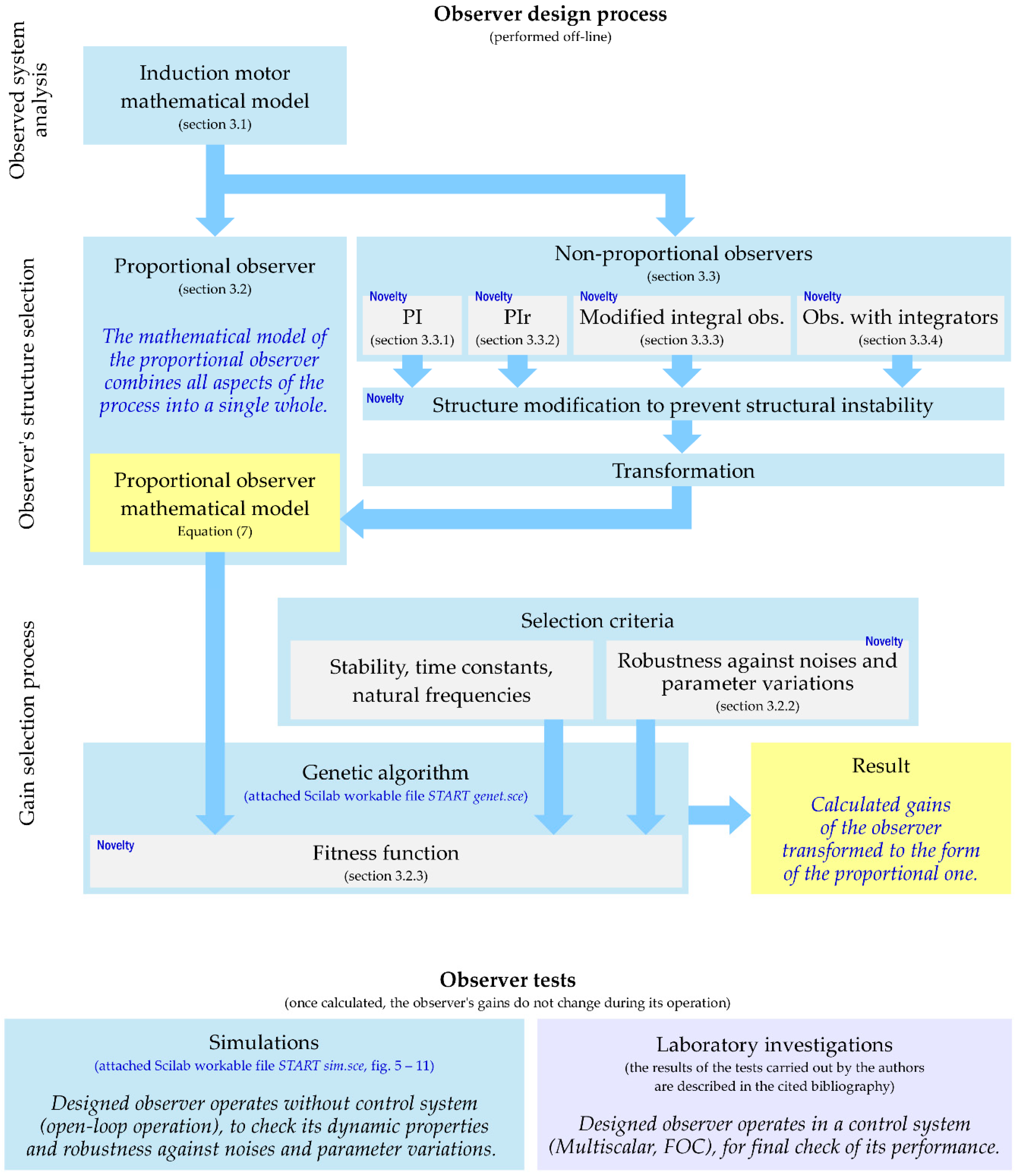
2. Methodology
In this paper, the selection of the gains of the proportional observer is described in its general form, which is also suitable for transformed non-proportional observers. The workflow of a proposed gain selection process is presented in Figure 1. The process starts with observed system (induction motor) mathematical model analysis, which is the base for the observer’s structure design. Next, the structure of the observer is chosen. If a non-proportional observer is chosen, then its structure must be modified, to prevent instability and transformed to the form of the proportional observer. Once the observer is transformed, its gains are to be optimized with a genetic algorithm. The transformation causes that the gain optimization is performed the same way, independently of the type of the observer. The described method may be applied with a program written in the Scilab environment as attached to this paper (Supplementary Materials, the START genet.sce file). The program in its original form is for gain selection of a proportional observer; however, it can also be applied for non-proportional observers. To do that, the matrices in lines 70–73 in the file START genet.sce are replaced with proper forms from lines 67–223 of the file START sim.sce. Also, the assumed structure of the gain matrix in lines 87–94 (START genet.sce) should be properly changed, to have the same sizes as gain matrices in lines 67–223 (START sim.sce).
The gain selection process is performed once, during observer design. Once calculated, the gains do not change during observer’s operation. The observers described in this paper may be tested with the attached simulation model (see the Scilab-Xcos file sim model.zcos). The simulation can be run with the START sim.sce file. The model is simplified, although it enables testing the observer’s performance in the presence of noises and parameter variations. It should be noted that such tests cannot be performed in the laboratory, since in a real electric drive, the values of noises and parameter variations are unknown. This is why simulations are so helpful. However, laboratory tests are the last step of the observer design process. The laboratory test results for the observers described in this paper can be found in previously published papers by the authors.
The observers’ gains optimized with the algorithm in the file START genet.sce may be tested with simulation started by the file START sim.sce. To do that, proper observer structure should be chosen in line 68 of the file START sim.sce, and new gains values should be typed in the appropriate places between lines 67–223. Both files may be used for induction motors that are different from the one used by the authors. The motor’s rated parameters and per-unit system base quantities may be changed in the file START genet.sce in lines 46–55 and in the file START sim.sce in lines 41–53. These values in both files should be the same.
3. Results
The observer design consists of two stages. In the first stage, the structure of the observer needs to be chosen based on the observed system mathematical model. In the second stage, the observer’s gains will be calculated. Both stages are combined together by a mathematical model of the proportional observer, based on a mathematical model of the motor.
3.1. Mathematical Model of the Motor
Let us take into consideration a linear dynamic system, described with the set of matrix equations [1,33,34]:
In case of an induction motor the state vector x, the input vector u and the output vector y have the following forms:
where ψ is the magnetic flux coupled with the motor’s winding, I is the current of the winding, and u is the winding voltage. Subscripts s and r refer to the stator and rotor windings, respectively. Subscripts α and β are also the axial components of the phasor in a stationary Cartesian coordinate system. In system (1), n = 4 state variables, p = 2 inputs and q = 2 outputs:
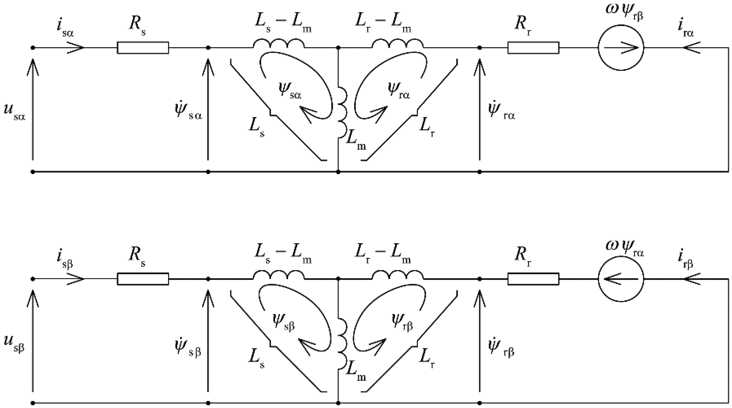
where Rs and Rr are the stator and rotor windings resistances respectively [33,34,35], Ls and Lr are the stator and rotor windings inductances, Lm is the magnetizing inductance, ω is the angular speed of the motor and 12 is the 2nd order identity matrix. All quantities in (1)–(4) are dimensionless, given as per-unit (p.u.) values. The per-unit system for AC machines is described in [36]. Equations (1)–(4) correspond to the equivalent circuit of an induction motor as presented in Figure 2.
Because the angular speed ω changes much slower than the electromagnetic variables u, i and ψ, it is treated as a parameter [1,33,35,37].
The forms of matrices A, B and C show that they are block matrices, built of two-row square matrices with a general form [25]:
where a and b are both real. Due to this fact, the angular speed ω always has an even power in the coefficients of the characteristic polynomial of the system (1):
where hi(ω2) is the i-th coefficient of the characteristic polynomial of the variable s. The order of the system (1) equals n = 2g. Hence, the sign of the angular speed has no impact on the dynamical properties of the system. It results from physical properties of the motor which operates in the same way independently of the rotation direction.
3.2. Proportional Observer and Its Gain Selection
The proportional observer is the most basic of all Luenberger observers. It is also a starting point for analyses and designs of more advanced observers. The operation principle is based on the assumption that the mathematical model of the system (1), driven with the same (measured) input signals u as the real motor, has similar values of the state variables x. Presumptive differences between real and calculated values, caused by disturbances and parameter variation, may be corrected based on the comparison of the real output signals y of the motor and the calculated. These differences are the measure of estimation errors, and signals proportional to these differences are utilized as correctional feedback. The gain matrix K is the factor of proportionality. Therefore, the proportional observer is described as follows [1,3,35]:
where (ˆ) denotes the quantity estimated by the observer. Matrix K has the dimensions n × q. Dynamical properties of the observer are evaluated based on its error equation. The error vector is defined by Equation (8):
The error equation of the proportional observer, derived from (1), (8) and (9) is given as [33]:
The state matrix E of the observer has the dimensions n × n. Equation (9) is the basis for the observer’s gain selection. The gains, being the elements of the matrix K, should be selected so that the observer was stable and had desired dynamical properties, described by time constants τ and natural frequencies f. The time constants and the natural frequencies are determined by the eigenvalues of the observer λ:
being the roots of the characteristic polynomial [3]:
The error Equation (9) has no input because it does not take into consideration any noises and parameter variations. Therefore, this equation only describes the process of attenuation of the errors, starting from the initial value ε0. This process occurs when the cause for error generation has already ceased.
3.2.1. Error Equation and Disturbances
If the output vector y of the system (1) has the number of elements q greater than 1, then the gain matrix K has more than one column. It can be proven [35,38] that in such a case the observer can have the same eigenvalues for the various matrix K element values. Moreover, in the observers having the same eigenvalues and different gains, identical disturbance can generate different errors. This problem may be analyzed with the help of the error equation that takes into consideration the disturbances as well.
Let us assume that the proportional observer (7) has been designed for the system (1), described with matrices A, B and C. However, because of parameter variations [39], the real system is described with the equation:
where ΔA, ΔB and ΔC are the matrices containing the parameter variations. The error equation derived for this case has the following form:
Therefore, parameter variations introduce two terms acting as the inputs to the error equation where one of them is dependent on the system (1) inputs u. In the case of the induction motor mathematical model (2), this term is not present as the elements of matrix B have the values 1 or 0 and no variations can occur. The other term is dependent on the state vector x and the gain matrix K. Therefore, it should be expected that the error values ε will be higher when the observer gains are higher.
Error occurrence may also be caused by disturbances overlaying the inputs u passed to the observer. It is assumed that the observer (7) has been designed for the system (1), but the input of the observer is supplied with signals containing the disturbances δu:
The resulting error equation has the following form:
The error Equation (15) contains an input dependent on the disturbances and independent of the observer’s gains.
The last cause for error occurrence is the disturbances overlaying the outputs of the system (1). If it is assumed that disturbance signals δy are transmitted through the observer via outputs y, then:
In this case, the error equation input is dependent on the observer gain matrix K:
The three error equations of (13), (15) and (17) are derived by taking into consideration all three previously listed error sources. In the case of (13) and (17), the observer’s gains have a direct impact on the generated errors. Therefore, the proper selection of gains may improve the estimation quality.
3.2.2. Amplification Index of the Observer
The most common tool for the analyses of the phenomena described in the previous section is the sensitivity theory which is used in [40] to evaluate the observers with selected gains. However, such analysis is complicated and requires a significant amount of numerical calculations. The results are also difficult to interpret. That makes it inadequate for the needs of the gain selection process, where processed gains have to be evaluated many times. Therefore, it is vital to find an alternative method as proposed by the authors (based on the experimental observations and numerical simulations). A new factor is proposed as the amplification index of the observer which is defined by the following equation:
where Kw,k is the element of the matrix K placed in the row number w and the column number k.
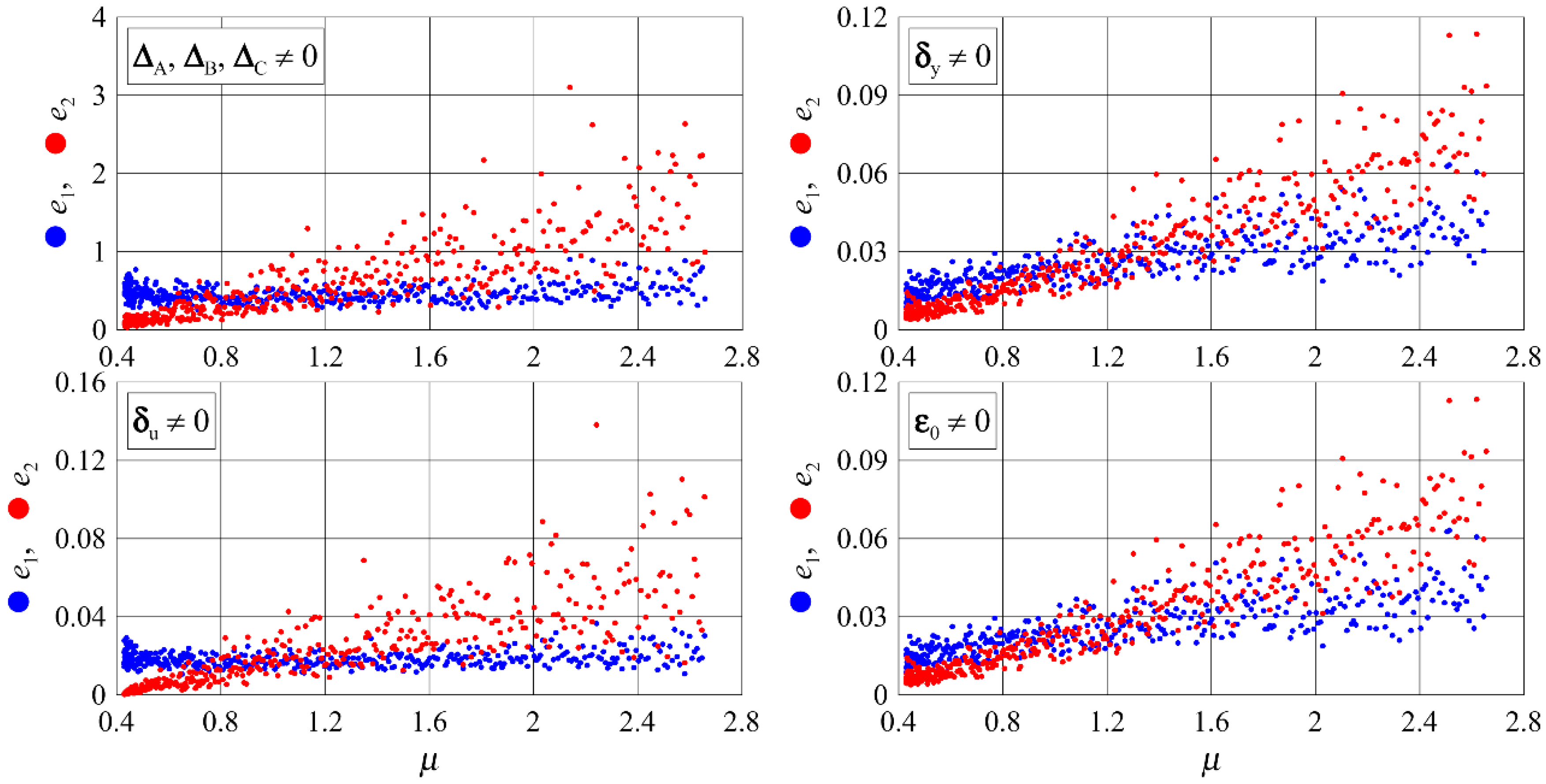
The correlation between the value of the amplification index μ and the values of errors generated by noises and parameter variations is exemplified by the results of simulations performed for the proportional observer (7), designed for an exemplary 2nd order linear system (1).
Simulations for 400 sets of observer’s gains were performed with four simulations for each set. Each matrix K contained one different set of gains, but provided the same eigenvalues of the observer. The first part of the four simulations was performed for parameter variations ΔA, ΔB and ΔC, with all other disturbances equal to zero. The second part was performed for the disturbances δu, and the third and fourth sets were performed for the disturbances δy and the initial values of errors ε0 (≠0), respectively. Each simulation generated two values of mean square errors e1 and e2 for both state variables of the system:
where T is the simulation total time. The results are presented in Figure 3. In cases ΔA, ΔB, ΔC ≠ 0 and δy ≠ 0, the error equation inputs directly depend on the values of the observer’s gains. An increase in the gain values also causes the values of e1 and e2 errors to be increased. A similar effect is also visible where δu ≠ 0, corresponding to the error Equation (15). This may be surprising as the input in Equation (15) does not depend on the matrix K. This effect is explained by the case ε0 ≠ 0, that describes the process of error attenuation, independent of the reason that caused the errors.
The general conclusion is that a higher estimation error is caused when the amplification index is higher. This conclusion is sufficient to propose a new gain selection criterion consisting of minimization of the value of μ. The value of μ can be easily calculated based only on the element values of the gain matrix K; therefore, this criterion does not introduce significant numerical costs.
3.2.3. Optimization Gain Selection
The gains of the observer were optimized using a genetic algorithm. Three different optimization criteria were applied. The first and the most important criterion is the proper placement of the observer’s eigenvalues (10) in the complex plane [25]. This criterion provides stability and desired dynamical properties of the observer. It should be noticed that based on (3), (9) and (11), the eigenvalues of the observer are parametrically dependent on the angular speed of the motor ω. This criterion is represented by the applied fitness function.
The second criterion is that the dynamical properties of the observer should be independent of the rotation direction of the motor. To meet this condition, matrix K must have the general form described with (5). This enforces reciprocal dependencies between the element values of the matrix K that have been applied.
The third criterion consists of minimization of the amplification index μ and increases the observer’s robustness. It was applied with the proper limitations of the search space, as well as with the additional term of the fitness function.
Applied fitness function F has a nonnegative value, the greater the value, the more distant is the solution from the ideal one:
where Fi is the subsequent components and wi are the nonnegative weight coefficients. Such a function always has a minimum, which should be found using the optimization process.
The following components of the fitness function were applied. The first category of the components relates to the real parts of the eigenvalues with the following form:
The F1 function has nonzero values when one or more of the eigenvalues has a positive real part. This component prevents the observer from instability.
The next component that ensures the stability has the value proportional to the positive real parts of the eigenvalues:
The fitness function also contains a term whose value is proportional to the difference between the real and the desired (reference) parts of the observer’s eigenvalues:
where the reference value λref may depend on the angular speed of the motor:
where cm is the constant coefficient. The polynomial (24) contains only even powers of the angular speed, ensuring that the sign of the angular speed has no impact on the value.
The next component has a similar form to F3, but is only calculated for the smallest real value:
The reference value λref is of the same form as (24), but is described with another set of parameters cm, so the polynomial may have a different value and order.
The components F5 and F6 determine the lower and the upper limit for all real parts of the eigenvalues:
The second category of the fitness function terms refers to the imaginary parts of the eigenvalues. The component F7 has the following form:
The next component assumes non zero values when the modules of the imaginary parts exceed the reference value:
The last component of the fitness function relates to the disturbance robustness criterion:
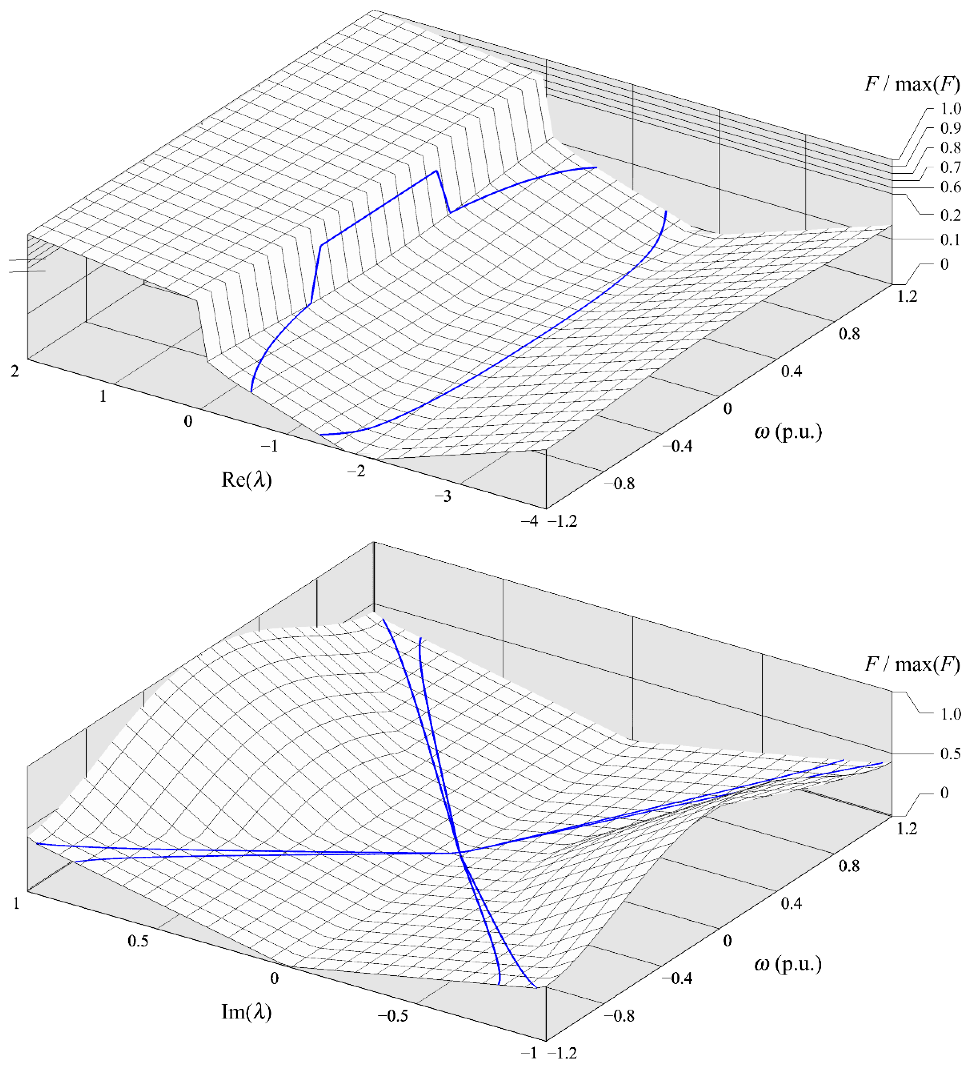
The weight coefficients in (20) and the reference values λref were experimentally adjusted, based on the repeatedly performed gain selection process and simulations. An exemplary set of the values that led to satisfying results is presented in Table 1. Fitness function values corresponding to the coefficients given in Table 1 are shown in Figure 4. This function was applied to the gain selection of a proportional observer of an induction motor rated at 7.5 kW; all simulations presented further in this paper were performed for this motor. The eigenvalues of the observer as the result of the selection process, are plotted on the surfaces as shown in Figure 4. The same results are presented in Figure 6 in the form of plots of real and imaginary parts of eigenvalues.
We tried to find the minimum of the fitness function using a genetic algorithm. The genetic algorithm was chosen because of its high efficiency in finding a global extremum of the fitness function [41]. It is very important in case of proposed fitness function (20)–(30), because its properties, e.g., number of local extrema, may depend on assumed weight coefficients wi in (20), as well as the reference values λref of terms (23), (25)–(27) and (29). In the case of deterministic algorithms, which of the local extrema is found largely depends on the starting point. In the case of the optimization problem under consideration, it is difficult to identify a starting point that guarantees a good result. The genetic algorithm guarantees a high probability of finding the global extremum because its starting population is evenly (with the same probability) distributed throughout the search space. The genetic algorithm also requires minimal information about the fitness function. In particular, unlike some deterministic optimization algorithms, it does not require knowledge of its derivative value. Computing the derivative of the fitness function would be troublesome in the present case due to the conditional structure of the components (21), (22), (26), (27) and (29).
The genetic algorithm operates on the basis of random numbers; therefore, each renewed run proceeds in a different way, and the optimization process is not always successful. Its most important disadvantage is the lack of result repeatability.
The population consisted of 500 chromosomes. The optimization process was stopped on the 25th generation. The chromosomes were based on floating-point coding. A proportional crossing-over, roulette-wheel selection and uniform random number one-point mutation were applied.
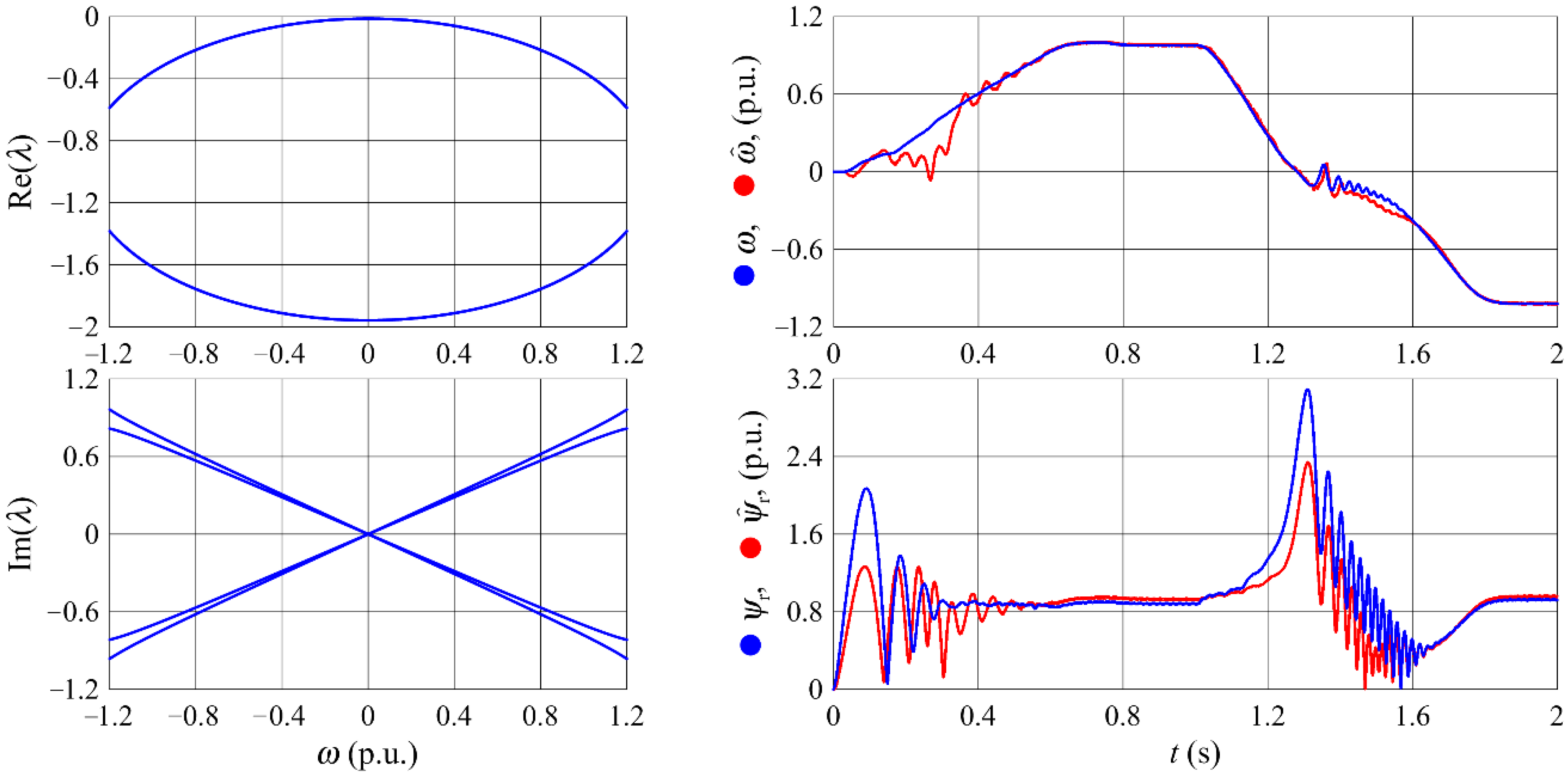
The results of numerous experiments with the genetic algorithm show that, in most cases, the convergence was reached before the 20th generation. The fitness function (20) has a complicated form and it is difficult to find whether it has one or several local minimum points. On the other hand, the algorithm launched several times for the same parameters of the function (20) but different initial generations, randomly generated and uniformly distributed in the search space, returned gain sets that were close to each other. Therefore, it can be assumed that if the function has more than one minimum, the algorithm finds the global one efficiently. The designed observer has been tested in simulation model presented in Figure 5. The simulation results obtained for the proportional observer designed with the presented method are shown in Figure 6. The experimental results are described in [35].
3.3. Non-Proportional Observers
Non-proportional observers described here contain additional dynamical units in their feedbacks. They provide stronger estimation error attenuation, increasing the robustness of the observer; however, they generate some problems. The first problem is that the observers have more state variables than the observed system (1). Therefore gain selection of such observers is more difficult than that of the proportional observer. Another problem is the structural instability of the observer that may occur for a certain class of observed systems.
3.3.1. Proportional-Integral Observer
In the proportional observer, the correction feedback signal has the value proportional to the estimation error. Therefore, if the error is constant in time, the feedback signal is also constant. Stronger correction may be achieved by introducing the dependence of the feedback signal on time. Proportional-integral (PI) observer has this ability [42,43,44,45]. The correction feedback signal in PI observer increases as long as the error differs from zero.
The PI observer is described with the set of equations:
where KP and KI are the gain matrices of the proportional and integral unit respectively. From (31) follows that two different sets of state variables are integrated in this observer. The first one is the set of estimated state variables of the system (1). These variables are associated with the state variable values of system (1), with the error Equation (9). Therefore, as long as the observer is stable, these values asymptotically approach the state variables values of the system (1). The second set of observer’s state variables, which are included in the vector h, are related to the feedback of the observer and are independent of the state variables of system (1). Therefore, they may assume potentially unlimited values, even if the observer is stable. This problem occurs especially when the input signals of the observer contain a constant component, introduced, for example, by a zero drift of a measurement instrument. In such a case the constant component is cumulated and the values of the feedback signals h gradually rise to infinity. This leads to some numerical problems.
Another problem is caused by those eigenvalues introduced by the feedback integrator, which are equal to zero. It is proven [31] that this may result in the structural instability of the observer in some cases, and it is impossible to correct with the observer’s gains.
Such problems occur in the PI observer as well as in other non-proportional observers which will be described later in this paper. To solve these problems, the mathematical model of the classical PI observer has been enhanced with the term—Ωh that was added to the second equation of (31). This change replaces the feedback integrator with the first-order inertia. The diagonal matrix Ω contains the inverses of the nonnegative inertia time constants. This additional term limits the values of the integrated state variables h and moves the eigenvalues related to the feedback to the left-hand part of the complex plane. The results show that the inertia time constants should be approximately ten times greater than the time constants (10) of the observer. Then, the correction of the observer’s feedback dynamical properties slightly affects the dynamical properties of the observer as a whole.
The gain selection of the PI observer is performed for its mathematical model derived in the form of the proportional observer mathematical model (7). The derivation requires the introduction of a new state vector of the PI observer:
Resulting matrices of the derived mathematical model have the following forms:
In the next step, matrices (33) and (34) are applied for the gain selection, which is performed in the same way as for the proportional observer.
3.3.2. Reduced Order Integral Unit PI Observer
A classical PI observer described with (31) has twice the number of state variables than the observed system (1). In the case of the induction motor observer, this number is equal to eight. The gain selection process for the observer of that high order is difficult from a numerical point of view. Therefore, it is advisable to find a structure of lower order which can be easier applied, but still offers a stronger error attenuation than the proportional observer. An intermediate structure between the proportional and the PI observers is a reduced order integral unit PI observer (PIr) [46,47], described with the following equations:
where G is the integral unit order reduction matrix. The matrix G has a lower number of columns than rows. Therefore, the number of elements of h vector is smaller than the number of elements in x vector.
The form of the matrix G may be defined in many ways. For the sake of the induction motor observer, the assumed form is consistent with the general rule (5):
The resulting PIr observer has six state variables, versus four state variables for the proportional observer and eight for the classical PI observer. The same way as for PI observer, the PIr observer has to be derived to the form of the proportional observer. An assumed new state vector and a new gain matrix are of the same forms as the PI observer (32) and (34). The resulting matrices of the mathematical model derived to the proportional observer form may be expressed as follows:
The gain selection and simulation results are shown in Figure 8.
3.3.3. Modified Integral Observer
The outcome of the error equation of the proportional observer (17) is that the observer tends to amplify the disturbances overlaying system (1) outputs. The modified integral observer [42] is free of this weakness. It is described with the following set of equations:
In this type of observer, the outputs of the observed system (1) are integrated, in contrast to the previous observers, where the difference between the real and estimated outputs are integrated. The first of Equations (38) has the same form as Equation (7) describing the proportional observer. Therefore, it is directly applied for gain selection purposes. To derive the forms of Ao, Bo and Co matrices, the following steps need to be performed. First, the second part of Equations (38) should be moved to the mathematical model of the observed system (1), and both equations should be merged, defining the new state vector of the observed system xo. This vector and the corresponding state vector of the observer (38) have the following forms:
Thereafter, for the new observed system mathematical model, a proportional observer should be designed. This leads to the following matrices:
The last step consists of moving the second part of Equations (38) back to the mathematical model of the observer.
The advantages due to the structure of the modified integral observer become visible on the derivation of its error equation, taking into consideration the disturbances δy overlaying the outputs of the system (1):
Comparing Equations (17) and (41) shows that in the case of the modified integral observer, the disturbances are not multiplied by the observer’s gains.
3.3.4. A Proportional Observer with Additional Integrators
All the observers described in this paper are based on the same mathematical model of the observed system as described with (1). The mathematical model of the observed system may also be defined in different ways, e.g., taking into consideration the disturbances, treated as unknown inputs.
The observers of the state variables of the induction motor very often operate provided with a speed adaptation mechanism, that estimates the angular speed ω of the motor [1,35]. The mechanism includes calculating the speed value on the base of the magnetic fluxes values, which is estimated by the observer. In such a case, the assumption made for the mathematical model (1), that the angular speed changes much slower than the other state variables and may be treated as a parameter, is no longer valid. However, this assumption is necessary to treat the induction motor as a linear system, therefore, it applicable [1,35]. A solution to this problem has not been found so far.
A partial solution for this problem may be the decomposition of the estimated speed signal into two components, a slowly varying actual speed ω and a quickly varying speed estimation error δω, that will be treated as an unknown input [35,48]. Let us assume that the estimated angular speed is input to the observer:
Then let us introduce Equation (42) into the mathematical model of the observed system (1)–(3) and define the unknown input vector d, that has z = 2 elements:
The state variables of the observed system described with (43) may be estimated with an observer with additional integrators [31,35,48]. It is a proportional observer (2) with feedback enhanced with the set of v additional integrators. The integrators generate an additional correction signal that is input to the copy of the observed system, being the part of the observer, as a replacement of the unknown inputs. The observer with the additional integrator is described with the following set of equations. The number of these equations depends on the number of additional integrators:
where the gain matrices of the additional integrators are shown as K1 to Kv.
The set of equations presented above in (45) may be derived to the form (7) on the definition of a new observer’s state vector:
Further derivations lead to the forms of the matrices:
The error equation of the observer with the additional integrators derived from (43) and (45) assumes the form:
The equation contains an input that equals the difference of the unknown input vector d and the correction signal generated by the set of the additional integrators.
In the case of the induction motor, the mathematical model (43) is used only in the observer’s design process. Once designed, the observer reconstructs the state variables of the system (1), the same as for all other observers presented in this paper.
The number of the additional integrators v is arbitrary and the greater it is, the stronger the compensation of the unknown inputs d. However, it should be noticed that each additional integrator introduced increases the number of the observer’s state variables by z = 2, making the gain selection process more difficult.
4. Discussion
Practical application of the non-proportional observers encounters problems that need to be solved to provide proper operation. First of all, when the number of the state variables of the observer is greater than the number of the state variables of the observed system, it may be necessary to modify the observer’s structure to provide stability. Despite this problem, the application of the observer with extended non-proportional feedback may provide better estimation quality than the application of the classical proportional observer.
Another problem is the proper gain selection. Two observers of the same structure and eigenvalues may have different gains and result in different robustness. Simulation results were presented in this paper for comparison purposes. These results were obtained under identical conditions for all presented observer structures. Presented observers were also successfully tested in the laboratory and results have been presented in the cited bibliography. Therefore, all of them are applicable in control systems of an induction motor.
All discussed observers were tested using the simulation model presented in Figure 5, in the same conditions, i.e., the introduced noises and motor’s parameter variations. The observers operated provided with a speed-adaptation mechanism [1,35,40]. The motor was fed with the voltage generated according to V/Hz = constant rule by a PWM power inverter. The observer’s inputs are passed reference voltages usαref and usβref, generated by the control system (sine waves), whereas the motor was fed with phase voltages based on those parameters but generated with PWM method (square waves). In the model of the motor, parameter variations were introduced. All the results were obtained with the same simulation model attached to this paper (Supplementary Materials, the START sim.sce file). For consecutive observers only the matrices of the observer’s simulation model were replaced. This also concerned the non-proportional observers described in Section 3.3. Therefore, the inner structure of the observer’s block was always the same. The waveforms illustrated three consecutive transient states, the start-up (0–0.5 s), the step switching on of the load torque (0.75 s) and the reversal (1–1.8 s). The load torque was active; therefore, the motor operated as a generator for negative speed values. The values of the state variables of the motor were given as dimensionless p.u. values [36].
Simulation results of the proportional observer are presented in Figure 6. It shows that the observer has relatively small real parts of the eigenvalues λ, which are smaller than the non-proportional observers described in Section 3.3. It means that the time constants of the proportional observer are shortest; nevertheless, this observer does not provide the best estimation quality. The reconstruction quality of magnetic fluxes has an impact on the operation of the speed adaptation mechanism; therefore the transient of the estimated angular speed ω (Figure 6) is a good measure of the observer’s performance. In this case, a significant difference between the real and estimated speed values is visible during the start-up of the motor (t = 0.3 s). Some small differences are also visible during the reversal of the motor (t from 1.3 to 1.6 s). It should be noted that the reversal (the change of rotation direction) of the motor is the most difficult state of operation from the observer’s point of view. In this state, the variations of the equivalent circuit parameters have the greatest impact on the estimation quality (especially variations of the stator and rotor windings resistances Rs and Rr). Moreover, during the reversal, the angular speed ω crosses 0. From the equivalent circuit (Figure 2) and the state matrix A (3) of the system (1), it can be seen that at the moment when ω = 0, the mathematical model divides into two subsystems that are not coupled with each other. The lack of coupling between the state variables deteriorates the operation of the observer’s feedback. This is why the reversal is a good test for the observer’s performance and robustness.
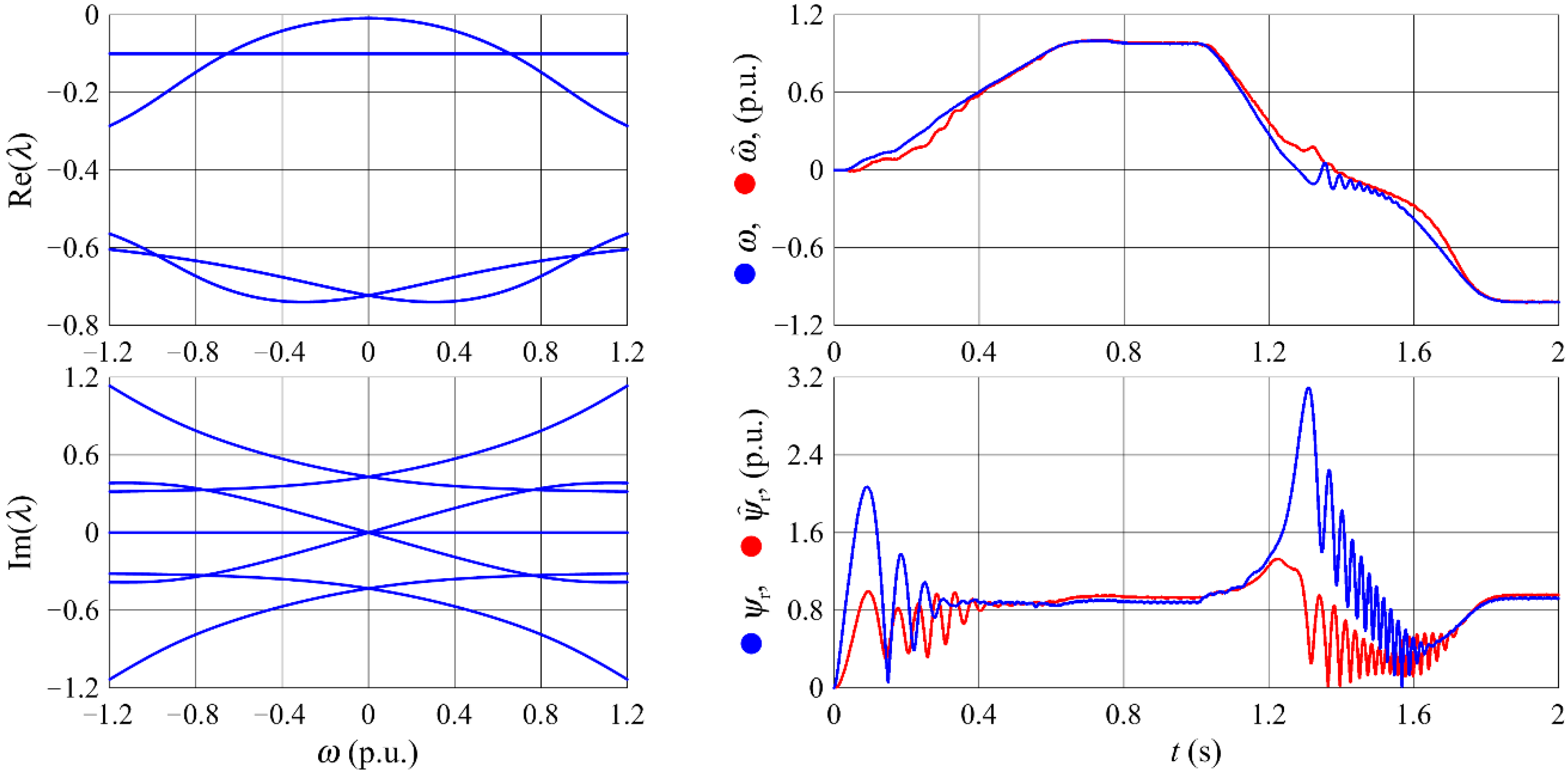
The PI observer (Section 3.3.1, Figure 7) has much longer time constants than the proportional observer described in Section 3.2. Nevertheless, its performance is slightly better. The weaker error attenuation, resulting from longer time constants, is compensated by structurally stronger feedback. The PI observer operates much better during the startup—angular speed estimation errors are smaller, although the performance during the reversal is slightly weaker. On the other hand, the selection of the gains is much more difficult in the case of the PI observer compared to the proportional observer. The problem results from the fact that the PI observer’s matrix Ao (33) is twice the size of matrix A (3) of the proportional observer. Also, the gain matrix K has twice the amount of elements.
The PIr observer (Section 3.3.2, Figure 8) has similar time constants as the PI observer described in Section 3.3.1, although it provides slightly better performance, especially during the reversal. The PIr observer is also better than the observers described in Section 3.3.3 and Section 3.3.4. The reduction of the integral unit has been proven to be a good compromise between the classical PI observer and the proportional observer. It combines the advantages of both of them, i.e., relatively simple structure and strong, proportional-integral feedback.
The modified integral observer (Section 3.3.3, Figure 9) is worse in comparison to the others described in this paper. The transient of the estimated angular speed in Figure 9 shows significant errors at all times, even in steady-state condition (t from 0.8 to 1 s). Potential gaining offered with less noise attenuation is dampened by disadvantageous results of replacing the integrator with the inertia. The replacement is necessary to provide observer stability, although it distorts the observed system’s outputs y passed to the observer. It is noticed that the outputs of the induction motor are sine-like waveforms; therefore, the impact of the inertia on them is significant. Therefore, this structure is not a good choice in cases of an induction motor, though its assets may be beneficial in other observed systems.
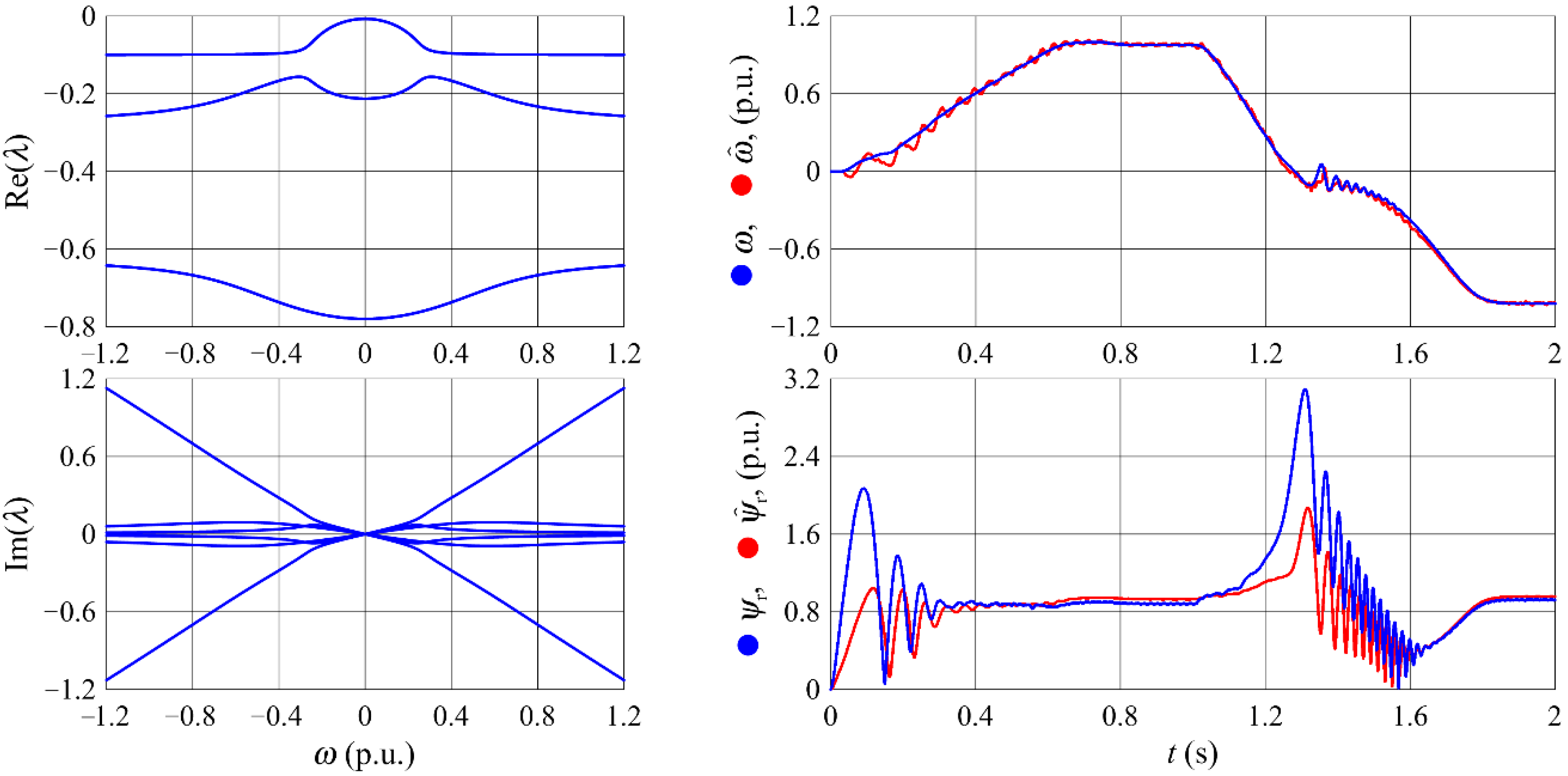
In the case of the observers with additional integrators (Section 3.3.4, Figure 10; Figure 11), the best results are achieved for v = 1 (Figure 10). Its operation during the reversal is as good as the PIr observer (Section 3.3.2), but its performance during the start-up is slightly weaker. The performance of both observers is similar, although the observer with an additional integrator has shorter time constants, resulting in stronger error attenuation. It means that the introduced additional integrator does not offer such possibilities as the proportional-integral feedback in the PIr observer. On the other hand, let us notice that the additional integrator is intended for attenuation of only one type of noise, the one overlying the angular speed.
Increasing the number of integrators up to v = 2 does not significantly improve the observer’s performance (Figure 11). The result for v = 2 is similar to that obtained for v = 1, but the observer with two additional integrators has a more complicated structure and as many state variables as the classical PI observer (Section 3.3.1). Based on that, it can be concluded that the application of more than one additional integrator is ungrounded. As the results obtained for v = 3 were even worse than for the previous two cases, the laboratory tests described in [35] were only performed for v equal to 1 and 2.
The PI and PIr observers, as well as the proportional observer with additional integrators, applied in the control system of an induction machine, provide better estimation quality at longer time constants than the proportional observer. Acceptable longer time constants mean that the displacement of the observer’s poles in the complex plane may be lesser in reference to the position of the motor’s poles. Lesser poles’ displacement results with lower gain values, making the observer more robust against noises and parameter variations.
Future research will be focused on improving the repeatability of the applied optimization method. Possible solutions are the application of other evolutionary strategies as firefly algorithms or simulated annealing as well as the application of a hybrid two-stage algorithm, where the first stage is an evolutionary one to find a global extrema and the second is a deterministic one to precisely locate the optimal solution [41]. Another goal for future research is finding criteria that will help to locate optimal settings of observers’ modified integrators contained in the matrix Ω.
5. Conclusions
Simulation and experimental tests demonstrated that the best estimation quality was provided by the classic PI and the PIr observers. However, the PI had a greater number of state variables and gains to select. Therefore, the gain selection process for this observer was the most difficult, i.e., it was difficult to find fitness function (20) parameters that ensured successful optimization. The proportional observer was the easiest to parametrize, so it was much easier to achieve satisfying estimation quality. However, it was not as good as in the case of the PI observer. The PIr observer with reduced order of integral unit and an observer with one additional integrator appeared to be a reasonable compromise between advanced structure and easy gain selection. They provided better estimation quality than the proportional observer and were easier to parametrize than the classical PI observer. The estimation quality of the modified integral observer was not satisfying. In particular, the changes introduced to its structure to provide its stability, deteriorated the estimation quality, especially for low supply voltage frequency and low angular speed of the motor. Therefore, we assert that this structure is not suitable for induction motor control systems and it is not recommended.
Supplementary Materials
The following are available online at https://www.mdpi.com/1996-1073/13/20/5487/s1, zip archive: sim_and_genet.zip. The archive contains the workable Scilab-Xcos simulation model that produced results shown in Figure 6, Figure 7, Figure 8, Figure 9, Figure 10 and Figure 11. The archive also contains the workable genetic algorithm for proportional observer gains selection that can be easily adjusted to gain selection of non-proportional observers presented in Section 3.3. See the read me.txt file for more details.
Author Contributions
Conceptualization, T.B.; methodology, T.B., R.N. and M.P.; software, T.B.; investigation, T.B. and R.N; writing—original draft preparation, T.B.; writing—review and editing, T.B., R.N. and M.P.; visualization, T.B.; supervision, M.P. All authors have read and agreed to the published version of the manuscript.
Funding
This research received no external funding.
Conflicts of Interest
The authors declare no conflict of interest.
References
- Kubota, H.; Matsuse, K.; Nakano, T. DSP-based speed adaptive flux observer of induction motor. IEEE Trans. Ind. Appl. 1993, 27, 344–348. [Google Scholar] [CrossRef]
- Auger, F.; Hilairet, M.; Guerrero, J.M.; Monmasson, E.; Orlowska-Kowalska, T.; Katsura, S. Industrial applications of the Kalman filter: A review. IEEE Trans. Ind. Electron. 2013, 60, 5458–5471. [Google Scholar] [CrossRef] [Green Version]
- Urbański, K. Determining the observer parameters for back EMF estimation for selected types of electrical motors. Bull. Pol. Acad. Sci. Tech. Sci. 2017, 65, 439–447. [Google Scholar] [CrossRef] [Green Version]
- Kazmierkowski, M.P.; Franquelo, L.G.; Rodriguez, J.; Perez, M.A.I.; Leon, J.I. High-Performance Motor Drives. IEEE Ind. Electron. Mag. 2011, 5, 6–26. [Google Scholar] [CrossRef] [Green Version]
- Kennel, R.; Rodriguez, J.; Espinoza, J.; Trincado, M. High Performance Speed Control Methods for Electrical Machines: An Assessment. In Proceedings of the IEEE International Conference on Industrial Technology, Vina del Mar, Chile, 14–17 March 2010; pp. 1793–1799. [Google Scholar]
- Rodriguez, J.; Kennel, R.M.; Espinoza, J.R.; Trincado, M.; Silva, C.A.; Rojas, C.A. High-Performance Control Strategies for Electrical Drives: An Experimental Assessment. IEEE Trans. Ind. Electron. 2012, 59, 812–820. [Google Scholar] [CrossRef]
- Wang, F.; Zhang, Z.; Mei, X.; Rodríguez, J.; Kennel, R. Advanced Control Strategies of Induction Machine: Field Oriented Control, Direct Torque Control and Model Predictive Control. Energies 2018, 11, 120. [Google Scholar] [CrossRef] [Green Version]
- Geyer, T.; Papafotiou, G.; Morari, M. Model Predictive Direct Torque Control—Part I: Concept, Algorithm, and Analysis. IEEE Trans. Ind. Electron. 2009, 56, 1894–1905. [Google Scholar] [CrossRef]
- Papafotiou, G.; Kley, J.; Papadopoulos, K.G.; Bohren, P.; Morari, M. Model Predictive Direct Torque Control—Part II: Implementation and Experimental Evaluation. IEEE Trans. Ind. Electron. 2009, 56, 1906–1915. [Google Scholar] [CrossRef]
- Wang, F.; Li, S.; Mei, X.; Xie, W.; Rodríguez, J.; Kennel, R.M. Model-Based Predictive Direct Control Strategies for Electrical Drives: An Experimental Evaluation of PTC and PCC Methods. IEEE Trans. Ind. Inf. 2015, 11, 671–681. [Google Scholar] [CrossRef]
- Karlovsky, P.; Lipcak, O.; Bauer, J. Iron Loss Minimization Strategy for Predictive Torque Control of Induction Motor. MDPI Electron. 2020, 9, 566. [Google Scholar] [CrossRef] [Green Version]
- Xinghua, Z.; Houbei, Z.; Zhenxing, S. Efficiency Optimization of Direct Torque Controlled Induction Motor Drives for Electric Vehicles. In Proceedings of the International Conference on Electrical Machines and Systems, Beijing, China, 20–23 August 2011; pp. 1–5. [Google Scholar]
- Khan, H.; Hussain, S.; Bazaz, M.A. Direct Torque Control of Induction Motor Drive with Flux Optimization. In Proceedings of the International Conference on Advances in Computing, Communications and Informatics (ICACCI), Kochi, India, 10–13 August 2015; pp. 618–623. [Google Scholar]
- Holtz, J. Sensorless Control of Induction Motor Drives. Proc. IEEE 2002, 90, 1359–1394. [Google Scholar] [CrossRef] [Green Version]
- Zaky, M.S.; Khater, M.; Yasin, H.; Shokralla, S.S. Review of different speed estimation schemes for sensorless induction motor drives. JEE 2008, 8, 102–140. [Google Scholar]
- Mousavi, S.M.; Dashti, G.A. Application of Speed Estimation Techniques for Induction Motor Drives in Electric Traction Industries and vehicles. Int. J. Automot. Eng. 2014, 4, 857–868. [Google Scholar]
- Wang, F.; Alireza Davari, S.; Chen, Z.; Zhang, Z.; Khaburi, D.A.; Rodríguez, J.; Kennel, R. Finite Control Set Model Predictive Torque Control of Induction Machine With a Robust, Adaptive Observer. IEEE Trans. Ind. Electron. 2017, 64, 2631–2641. [Google Scholar] [CrossRef]
- Ammar, A.; Kheldoun, A.; Metidji, B.; Ameid, T.; Azzoug, Y. Feedback linearization based sensorless direct torque control using stator flux MRAS-sliding mode observer for induction motor drive. ISA Trans. 2020, 98, 382–392. [Google Scholar] [CrossRef] [PubMed]
- Niestrój, R.; Białoń, T.; Pasko, M.; Michalak, J. Study of adaptive proportional observer of state variables of induction motor taking into consideration the generation mode. In Proceedings of the International Symposium on Electrical Machines (SME), Naleczow, Poland, 18–21 June 2017; pp. 1–6. [Google Scholar]
- Niestrój, R.; Białoń, T.; Pasko, M.; Lewicki, A. Selected dynamic properties of adaptive proportional observer of induction motor state variables. In Proceedings of the 13th Selected Issues of Electrical Engineering and Electronics (WZEE), Rzeszow, Poland, 4–8 May 2016; pp. 1–6. [Google Scholar]
- Zhang, Y.; Zhao, Z.; Lu, T.; Yuan, L.; Xu, W.; Zhu, J. A Comparative Study of Luenberger Observer, Sliding Mode Observer and Extended Kalman Filter for Sensorless Vector Control of Induction Motor Drives. In Proceedings of the IEEE Energy Conversion Congress and Exposition, San Jose, CA, USA, 20–24 September 2009; pp. 2466–2473. [Google Scholar]
- Cuibus, M.; Bostan, V.; Ambrosii, S.; Ilas, C.; Magureanu, R. Luenberger, Kalman and Neural Network Observers for Sensorless Induction Motor Control. In Proceedings of the IPEMC 2000. Third International Power Electronics and Motion Control Conference (IEEE Cat. No. 00EX435), Beijing, China, 15–18 August 2000. [Google Scholar]
- Harnefors, L. A comparison between directly parametrised observers and extended Kalman filters for sensorless induction motor drives. In Proceedings of the International Conference on Power Electronics and Variable Speed Drives, London, UK, 21–23 September 1998. [Google Scholar]
- Manes, C.; Parasiliti, F.; Tursini, M. A Comparative Study of Rotor Flux Estimation in Induction Motors with a Nonlinear Observer and the Extended Kalman Filter. In Proceedings of the IECON’94-20th Annual Conference of IEEE Industrial Electronics, Bologna, Italy, 5–9 September 1994; pp. 2149–2154. [Google Scholar]
- Pimkumwong, N.; Wang, M.S. Full-order observer for direct torque control of induction motor based on constant V/F control technique. ISA Trans. 2018, 73, 189–200. [Google Scholar] [CrossRef]
- Kadrine, A.; Tir, Z.; Malik, O.P.; Hamida, M.A.; Reatti, A.; Houari, A. Adaptive non-linear high gain observer based sensorless speed estimation of an induction motor. J. Franklin Inst. 2020, 357, 8995–9024. [Google Scholar] [CrossRef]
- Gao, Z.; Habetler, T.G.; Harley, R.G.; Colby, R.S. A Sensorless Adaptive Stator Winding Temperature Estimator for Mains-Fed Induction Machines with Continuous-Operation Periodic Duty Cycles. IEEE Trans. Ind. Appl. 2008, 5, 1533–1542. [Google Scholar]
- Espinoza-Trejo, D.R.; Campos-Delgado, D.U.; Martinez-Lopez, F.J. Variable Speed Evaluation of a Model-Based Fault Diagnosis Scheme for Induction Motor Drives. In Proceedings of the IEEE International Symposium on Industrial Electronics, Bari, Italy, 4–7 July 2010; pp. 2632–2637. [Google Scholar]
- Kim, H.S.; Lee, C.H.; Ahn, H.U.; Kim, S.B. Sensorless Speed Control of Induction motor Using observation Technique. J. Korean Soc. Mar. Eng. 1999, 1, 96–102. [Google Scholar]
- Gaddouna, B.; Ouladsine, M.; Rachid, A.; El Hajjaji, A. State Estimation of an Induction Machine using a Reduced Order PI Observer. In Proceedings of the Multiconference on Computational Engineering in Systems Applications IEEE Conf, CESA, Nabul-Hammamat, Tunisia, 1–4 April 1998; pp. 1022–1026. [Google Scholar]
- Białoń, T.; Lewicki, A.; Niestrój, R.; Pasko, M. Stability of a proportional observer with additional integrators on the example of the flux observer of induction motor. Electron. Rev. 2011, 87, 142–145. [Google Scholar]
- Hu, J.; Wu, B. New Integration Algorithms for Estimating Motor Flux over a Wide Speed Range. IEEE Trans. Power Electron. 1998, 5, 969–977. [Google Scholar]
- Toumi, D.; Segueir Boucherit, M.; Tadjine, M. Observer-based fault diagnosis and field oriented fault tolerant control of induction motor with stator inter-turn fault. Arch. Electron. Eng. 2012, 61, 165–188. [Google Scholar] [CrossRef]
- Krzemiński, Z.; Lewicki, A.; Morawiec, M. Speed observer based on extended model of induction machine. In Proceedings of the IEEE International Symposium on Industrial Electronics, Bari, Italy, 4–7 July 2010; pp. 3017–3112. [Google Scholar]
- Białoń, T.; Lewicki, A.; Pasko, M.; Niestrój, R. Non-proportional full-order Luenberger observers of induction motors. Arch. Electron. Eng. 2018, 67, 925–937. [Google Scholar]
- IEEE Standard Definitions of Basic Per Unit Quantities for Alternating-Current Rotating Machines; IEEE Std 86-1975; The Institute of Electrical and Electronics Engineers, Inc.: New York, NY, USA, 1975; pp. 1–10.
- Amrane, A.; Larabi, A.; Aitouche, A. Unknown input observer design for fault sensor estimation applied to induction machine. Math. Comput. Simul. 2020, 167, 415–428. [Google Scholar] [CrossRef]
- Ellis, G. Observers in Control Systems; Academic Press: Cambridge, MA, USA, 2002. [Google Scholar]
- Korbicz, J. Robust fault detection using analytical and soft computing methods. Bull. Pol. Acad. Sci. Tech. Sci. 2006, 54, 75–88. [Google Scholar]
- Niestrój, R. Analysis of selected dynamic properties of adaptive proportional observer of induction motor state variables. Q. Elektr. 2015, 61, 7–28. (In Polish) [Google Scholar]
- Francisco, M.; Revollar, S.; Vega, P.; Lamanna, R. A comparative study of deterministic and stochastic optimization methods for integrated design of processes. IFAC Proc. 2005, 38, 335–340. [Google Scholar] [CrossRef] [Green Version]
- Busawon, K.K.; Kabore, P. Disturbance attenuation using proportional integral observers. Int. J. Control 2001, 74, 618–627. [Google Scholar]
- Nazari, S.; Shafai, B. Distributed Proportional-Integral Observers for Fault Detection and Isolation. In Proceedings of the IEEE Conference on Decision and Control (CDC), Miami Beach, FL, USA, 17–19 December 2018; pp. 6328–6333. [Google Scholar]
- Białoń, T.; Lewicki, A.; Pasko, M.; Niestrój, R. Parameter selection of an adaptive PI state observer for an induction motor. Bull. Pol. Acad. Sci. Tech. Sci. 2013, 61, 599–603. [Google Scholar]
- Wang, X.T.; Yu, H.H. Generalized PI observer design for descriptor linear system. Arch. Control Sci. 2019, 29, 585–601. [Google Scholar]
- Hussein, A.A. Implementation of Proportional-Integral-Observer Techniques for Load Frequency Control of Power System. In Proceedings of the 8th International Conference on Ambient Systems, Networks and Technologies, ANT-2017 and the 7th International Conference on Sustainable Energy Information Technology, SEIT 2017, Madeira, Portugal, 16–19 May 2017; pp. 754–762. [Google Scholar]
- Hu, F.R.; Hu, J.S. Pole placement design of proportional-integral observer with stochastic perturbations. Eng. Comput. 2016, 33, 1729–1741. [Google Scholar] [CrossRef]
- Jiang, G.P.; Wang, S.P.; Song, W.Z. Design of observer with integrators for linear systems with unknown input disturbances. Electron. Lett. 2000, 36, 1168–1169. [Google Scholar] [CrossRef]
Figure 1.
Methodology workflow.

Figure 2.
The equivalent circuit of an induction motor in stationary Cartesian coordinate system α-β.
Figure 2.
The equivalent circuit of an induction motor in stationary Cartesian coordinate system α-β.

Figure 3.
The dependence of the estimation errors on the amplification index.

Figure 4.
The value of the fitness function versus eigenvalues of the observer and the angular speed of the motor.
Figure 4.
The value of the fitness function versus eigenvalues of the observer and the angular speed of the motor.

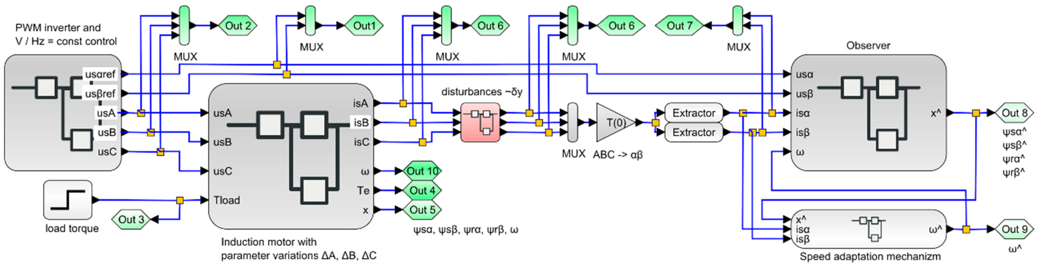
Figure 5.
Simulation model in Scilab-Xcos environment, simplified version. For full simulation model refer to attached file sim model.zcos.
Figure 5.
Simulation model in Scilab-Xcos environment, simplified version. For full simulation model refer to attached file sim model.zcos.

Figure 6.
The eigenvalues and simulation results obtained for the proportional observer.

Figure 7.
The eigenvalues and simulation results obtained for the PI observer.

Figure 8.
The eigenvalues and simulation results obtained for the PIr observer.

Figure 9.
The eigenvalues and simulation results obtained for the modified integral observer.

Figure 10.
The eigenvalues and simulation results obtained for the observer with one (v = 1) additional integrator.
Figure 10.
The eigenvalues and simulation results obtained for the observer with one (v = 1) additional integrator.

Figure 11.
The eigenvalues and simulation results obtained for the observer with two (v = 2) additional integrators.
Figure 11.
The eigenvalues and simulation results obtained for the observer with two (v = 2) additional integrators.


Table 1.
Fitness function coefficients applied for gain selection of the proportional observer.
| The Number of the Term Fi |
Weight Coefficient wi | Coefficients cm of the λref Polynomial m (24) | ||
|---|---|---|---|---|
| m = 0 | m = 2 | m = 4 | ||
| 1 | 20 | - | - | - |
| 2 | 1 | - | - | - |
| 3 | 1 | −2 | - | - |
| 4 | 1 | −0.96 | −0.96 | 0.32 |
| 5 | 1 | −0.195 | −0.065 | −0.0325 |
| 6 | 0.1 | −2.6 | 0.65 | −0.325 |
| 7 | 0.05 | - | - | - |
| 8 | 0.1 | 0.3 | 0.9 | −0.3 |
Publisher’s Note: MDPI stays neutral with regard to jurisdictional claims in published maps and institutional affiliations. |
© 2020 by the authors. Licensee MDPI, Basel, Switzerland. This article is an open access article distributed under the terms and conditions of the Creative Commons Attribution (CC BY) license (http://creativecommons.org/licenses/by/4.0/).
Share and Cite
MDPI and ACS Style
Białoń, T.; Pasko, M.; Niestrój, R. Developing Induction Motor State Observers with Increased Robustness. Energies 2020, 13, 5487. https://doi.org/10.3390/en13205487
AMA Style
Białoń T, Pasko M, Niestrój R. Developing Induction Motor State Observers with Increased Robustness. Energies. 2020; 13(20):5487. https://doi.org/10.3390/en13205487
Chicago/Turabian StyleBiałoń, Tadeusz, Marian Pasko, and Roman Niestrój. 2020. "Developing Induction Motor State Observers with Increased Robustness" Energies 13, no. 20: 5487. https://doi.org/10.3390/en13205487
Note that from the first issue of 2016, this journal uses article numbers instead of page numbers. See further details here.