An Implementation Method for an Inductive Proximity Sensor with an Attenuation Coefficient of 1 †


School of Information Engineering, Yangzhou University, Yangzhou 225100, China
*
Author to whom correspondence should be addressed.
†
This paper is an extended version of our paper published in Proceedings of 2020 Chinese Intelligent Systems Conference, Shenzhen, China, 24–26 October 2020; pp. 455–463.
Energies 2020, 13(24), 6482; https://doi.org/10.3390/en13246482
Submission received: 15 October 2020
/
Revised: 3 December 2020
/
Accepted: 3 December 2020
/
Published: 8 December 2020
Abstract
:In order to achieve long-distance measurement, a bridge differential inductance detection circuit is employed; on this basis, an automatic zero adjustment technique for sensors using an integral–proportional-integral controller is proposed in this work to achieve consistent product production and efficient installation and debugging, and the mathematical model of the bridge differential inductance detection circuit is established to effectively design the controller parameters. Furthermore, an implementation method for an inductive proximity sensor with an attenuation coefficient of 1 is also proposed based on the bridge differential inductance detection circuit by querying the proximity distance table in the field-programmable gate array (FPGA) to detect multiple target metal objects at the same inductive distance. Simulation and experimental results show that the proposed method is correct and effective.
1. Introduction
Since the beginning of the 21st century, there has been a growing demand for proximity sensors in various fields. Due to the various demands, proximity sensors have been developing in the direction of diversification. For different applications, proximity sensors should be selected to meet the specific requirements [1,2]. The proximity sensor is a kind of position sensor which can operate moving objects without contact. When the object is near the sensing surface of the sensor, it does not need mechanical contact or any pressure to make the sensor act. There are many types of proximity sensors, including those that use quartz crystal oscillators, and they are very accurate [3,4]. Because inductive proximity sensors have the advantages of a simple structure and strong anti-interference ability, the application of inductive proximity sensors is becoming increasingly extensive. With the development of aerospace and industry, high requirements are placed on the long-distance measurement of inductive proximity sensors [5].
In order to increase the measuring distance, the mechanical principle of a metal slope is used to realize the measurement of larger distances. The distance measuring ranges are small and strongly dependent on the sensor size. In addition, the sensors are not by themselves able to measure translatory movements of the target.To overcome this obstacle, users usually complete the system with a metal incline, which is rigidly coupled with the object. The large displacement is converted mechanically into a small change of the distance between the incline and the active face of the inductive proximity sensor. This method enables significant increases in the sensing range. The function of the incline is performed by a cone located on the device shaft. However, the advantages of inductive proximity sensors, such as linearity, accuracy and repeatability, need to find compromises with the slope conversion rate (usually 5–10). It can be seen that the method of using a mechanical slope to increase the detection distance is limited. In [6], the displacement of a target metal object is detected by means of a permanent magnet (auxiliary target), which increases the detection distance. However, the measurement target must be magnetic, which limits the types of objects that can be measured. Therefore, in [7], a detection method is studied which can not only eliminate the limitation of the mechanical conversion device and/or auxiliary magnet target but can also allow the inductive proximity sensor to achieve high performance. This method is realized according to the function relationship between the detection distance and transducer impedance (Z). However, it is difficult to describe the dependence of the transducer impedance on the transducer’s electrical and mechanical properties. Therefore, the relationship between the transducer impedance (Z), detection distance and operating frequency can only be reflected logically.
For long-distance measurement, a bridge differential inductance detection circuit is used in the measurement circuit of sensors in this paper [8]. The detection circuit detects the inductance variation of the coil in the induction surface to realize the measurement of the approach distance of the target metal objects. This method can eliminate most external interference signals and, as far as possible, ensure the effectiveness of the necessary information we need to enhance the anti-interference ability [9,10]. In order to achieve consistent product performance, in this paper, we propose an automatic zero calibration method for the foundation of an integral–proportional-integral (I-PI) controller on the basis of a bridge differential inductance detection circuit. Because the reference inductor in this paper needs to be adjustable, this method solves the problem of the difficulty of making the reference inductor [11].
At present, most inductive sensors adopt a measurement method based on an AC damping factor. This approach consists of an inductance coil and an external capacitance to form an oscillation detection circuit. The smaller the detection distance, the greater the damping coefficient and the smaller the amplitude of oscillation, and even the vibration is stopped.Therefore, the proximity of metal targets can be measured according to the oscillation amplitude. However, the RLC which is a series parallel circuit of resistance, inductance and capacitance of the transmission line will affect the frequency and amplitude of oscillation, which will lead to a decrease in the measurement accuracy. The method in this paper realizes the detection of all metal targets at the same distance, which has no attenuation to the measured material detection distance and does not need to be recalibrated for different materials. This method has high precision and stable performance. The inductance increment detection circuit can cancel the self-inductance of the detection coil by setting the bias inductance and then converting the equivalent inductance increment related to the proximity into an electric quantity. We can thus obtain the distance information of the corresponding metal target and meet the requirements of measurement accuracy. The capacitance range of traditional sensors such as capacitive sensors is very small, thus placing high requirements on the accuracy of capacitance detection. Especially in the process of sensor development, high-precision capacitance detection equipment is often required to test and calibrate the sensor. However, there is a lack of a special instrument for the real-time detection of micro capacitance in China and abroad. The common practice is to design and make a special capacitance detection circuit for the sensor, which undoubtedly increases the difficulty and workload of sensor design. In this paper, the I-PI automatic zero adjustment method is adopted, which is easy to use and reduces the error.
Based on the analysis of the bridge differential inductance detection circuit, a measurement method with an attenuation coefficient of 1 based on the field-programmable gate array (FPGA) is proposed, which can detect multiple metal objects at the same sensing distance.This is the attenuation coefficient of 1. When the common inductive proximity sensor detects metal objects of different materials, the detection distance will change. This is due to the different attenuation coefficients between different metals. When detecting objects made of different types of metals, different types of sensors must be used, which greatly increases the workload of staff and reduces the consistent reliability of products. A sensor with an attenuation coefficient of 1 solves these problems and unifies the switching distance of all metal types; that is, the switching distance is the same for all metal materials. This makes it unnecessary to replace new sensors when detecting the proximity of different metal objects, thus reducing the budget and costs. This paper first introduces the operating principle of inductive proximity sensors for long-distance measurement. On this basis, a small signal model from control voltage to bias inductance is established. An automatic zero calibration method based on an integral–proportional-integral (I-PI) controller is proposed, and the attenuation coefficient of 1 is achieved by searching in the table.
2. Operating Principle of Inductive Proximity Sensor
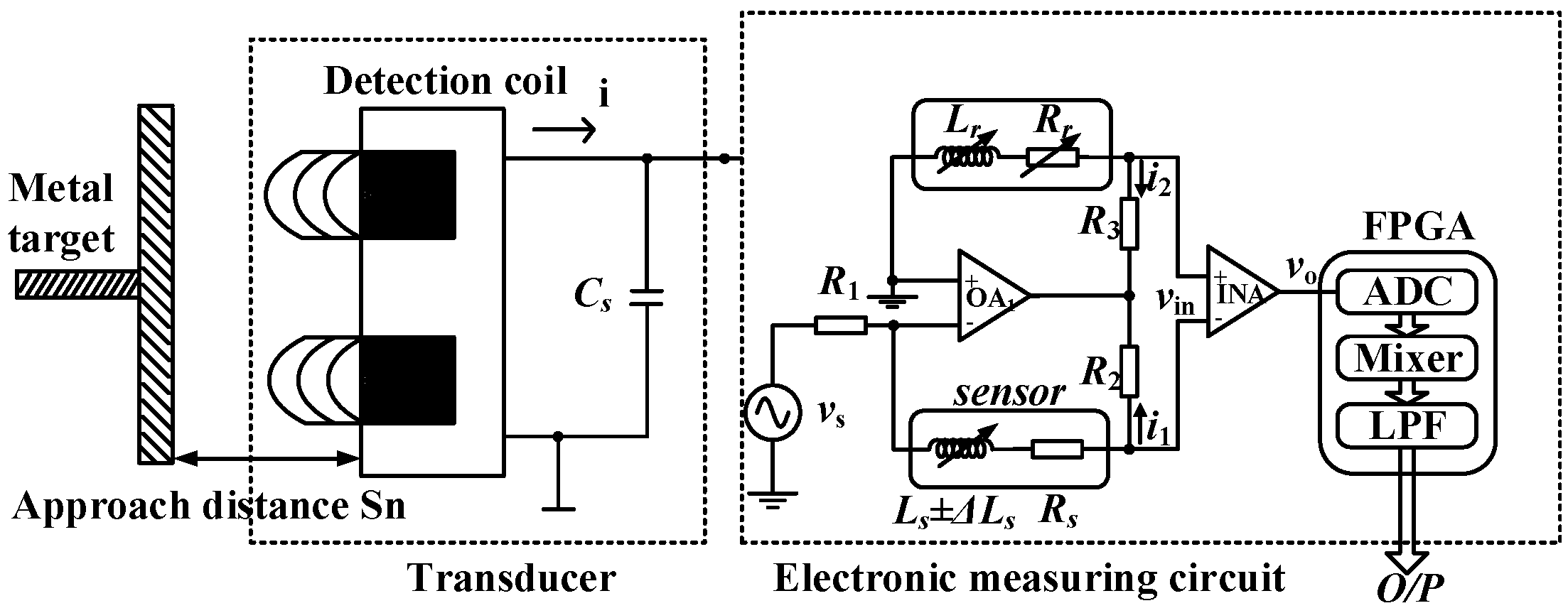
An inductive proximity sensor is composed of a primary side transducer (located on the sensing surface) and an electronic measuring circuit, as shown in Figure 1.
The primary transducer is actually made up of inductors and capacitors, which generate electromagnetic fields through the excitation oscillation current inside the sensor, thus forming an induction surface at the end face of the sensor [12,13]. When the approaching distance or motion information of the target metal object changes, the parameters of the primary side transducer will change, such as the quality factor and coil inductance. The electronic measurement circuit of the sensor outputs the corresponding control signal by detecting the change signal of oscillation circuit parameters. The control signal can be an analog quantity corresponding to the detection distance or it can be a switch signal.
2.1. Principle of Electronic Circuits
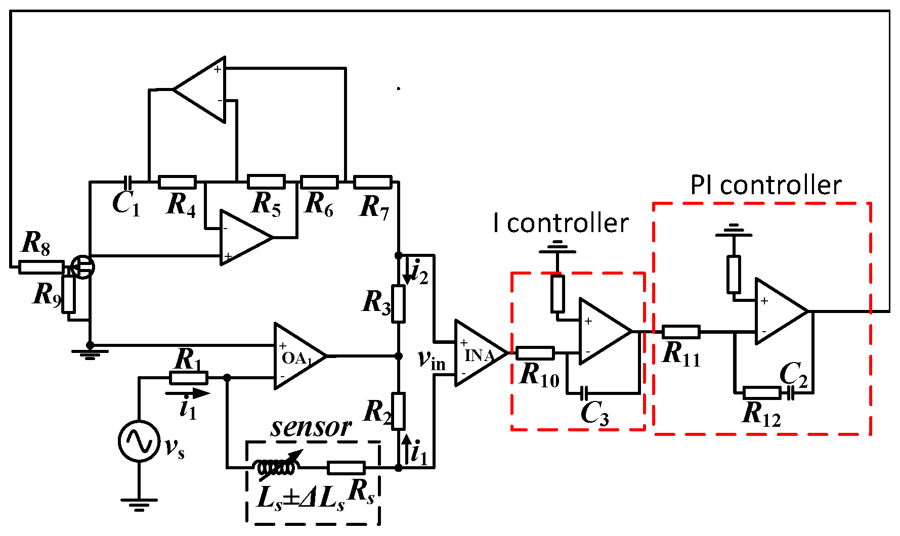
Due to the symmetry of the bridge arm, an AC bridge circuit is usually used as a detection circuit [14,15]. However, this method has limitations and will incur extra temperature drift [16,17]. Considering the common mode noise is effectively suppressed and the effective differential signal is retained in the differential circuit, the bridge circuit and differential detection circuit are combined in this paper, and the bridge differential inductance detection circuit is employed as shown in Figure 2.
When the object moves in the sensing range of the sensor, the inductance value of the coil will become larger or smaller, but this change is small relative to the inductance value of the coil itself. The change of inductance will lead to a change of output voltage. In this work, we use an instrument amplifier to amplify the output voltage to meet accuracy requirements in order to reflect the change of inductance more accurately and realize the distance measurement.
In Figure 2, is the high-frequency oscillation excitation source; its frequency is 1 kHz. is the current limiting resistance, OA1 is the operational amplifier; is the self-inductance; is the change of the coil inductance when the metal object is approaching; is the equivalent resistance; is the inductance value of the reference inductance; is the resistance value of the reference inductance; and are the matching resistance; INA is the instrument amplifier, where and are the input voltage and output voltage of the instrument amplifier, respectively; and and are the bridge arm current in the upper and lower bridge arms, respectively. The inductance and resistance are used in series to detect the inductance and resistance of the coil. We need to adjust the to equal before the targets move into the sensing range of sensors.
We adjust the value of to ensure that and are equal, and If the resistance is equal to and , then the input is zero, and the output of the amplifier is also zero [18]. When the metal object is near the sensing surface for a certain distance , the inductance changes and produces an increment . The output of the instrument amplifier is thus no longer zero. With the change of , will also change.The variable voltage signal is sent to the FPGA; according to the corresponding relationship between the approach distance of the sensor and the variable voltage, the approach distance of the target object is obtained.
2.1.1. Implementation of Bias Inductor
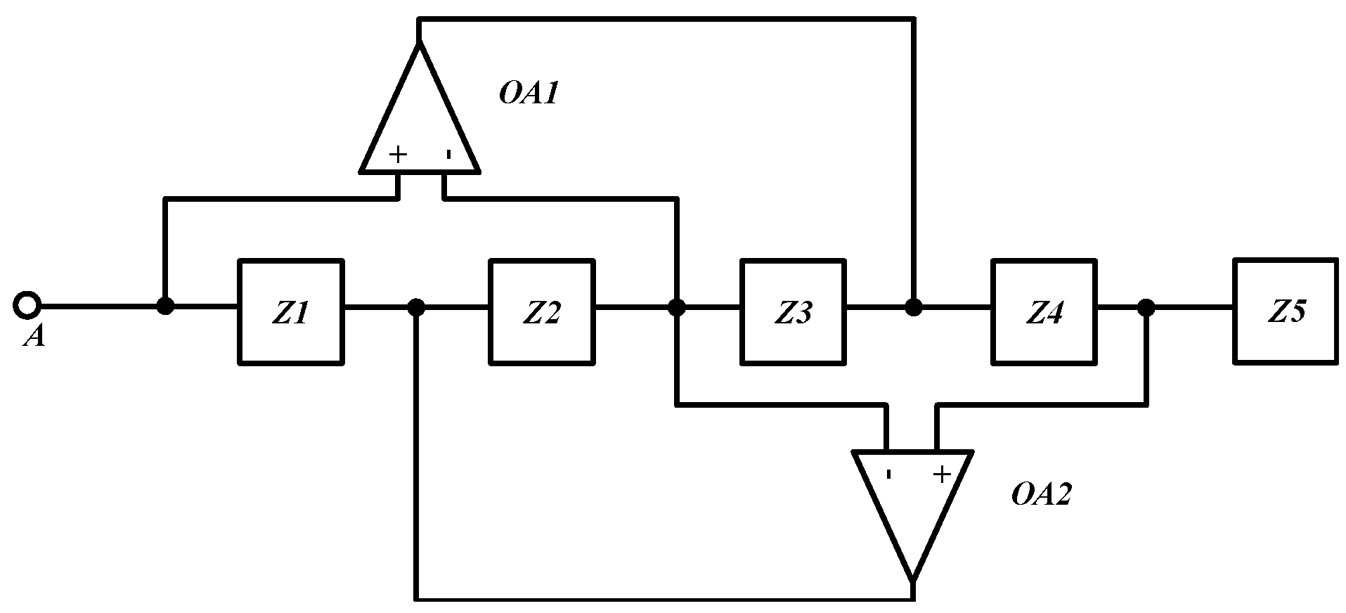
When the target metal object is not near the detection coil, the reference inductance value in the electronic measurement circuit should be equal to the detection coil inductance value, meaning that the output is zero. Otherwise, when the target metal is close to the induction head, the proximity distance cannot be reflected truly and the required measurement accuracy cannot be achieved. This requires that the reference inductance in the bridge differential detection circuit should be adjustable. In this paper, the equivalent inductance is realized by the general impedance converter shown in Figure 3 [19,20].
According to the virtual short and virtual break characteristics of the operational amplifier, we can obtain the equivalent impedance formula of the general impedance converter as follows:
When or are capacitors and other impedance elements are resistors, the general impedance converter can be equivalent to an analog inductance. Suppose that is a capacitor and , the formula is as follows:
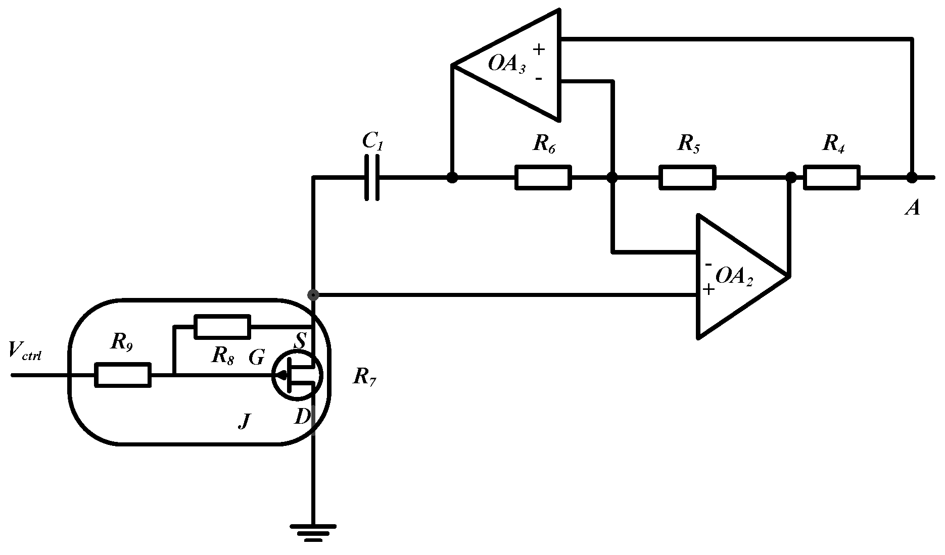
It can be seen that the general impedance converter can be equivalent to from point A. The general impedance converter has realized an equivalent reference inductance, and the inductance of the equivalent reference inductance is . The equivalent circuit diagram is shown in Figure 4.
It can be seen from Figure 4 that the inductance value of reference inductance can be adjusted by changing the value of . In order to realize that the value of resistance can be adjusted by the electronic control signal, this paper uses the junction field-effector transistor (JFET) to realize . The JFET is a voltage-controlled device, which does not need excessive signal power. It has a low noise figure and a wide-ranging variable resistance area. In this way, the specific value of the voltage-controlled resistance can be achieved by controlling the gate voltage of the JFET, where . When and near the JFET are equal, the linearity of the JFET can be effectively increased. The variable resistance value of the JFET is only related to the gate voltage and is not affected by the drain source voltage .
3. Principle of the Proposed Adaptive Zero Adjustment Technique
In the process of practical application, before the target metal enters the sensing range of the inductive proximity sensor, it is essential to adjust the to make Lr equal Ls. From Equation (3), we can adjust the applied to the JFET gate source to make the reference inductance equal to the measured inductance . Then, the input is zero and the output of the instrument amplifier is also zero, which is called zero adjustment. After zeroing, the must be kept unchanged, and the inductance value of the reference inductor remains unchanged. When the metal object enters the sensing range of the sensor, the inductance of the coil will vary and the increment will be generated. and the output of the instrument amplifier will no longer be 0. The will be sent to the FPGA of the later stage for processing so that the approach distance of the target can be obtained according to the variation of inductance. The distance measurement of the target metal object is thus realized.
If the sensor has not been zeroed—that is, the reference inductance in the electronic measurement circuit is not equal to the value of of the detected coil—when the target metal is far away from the sensing range of the sensor, will not be equal to zero and the amplified signal of the instrument amplifier will certainly not be equal to zero. This can lead to inaccurate distance measurement. In order to realize the automatic zero adjustment of the sensor, it is known from control theory that closed-loop negative feedback control must be implemented for the control quantity [21,22]. The control quantity here is the signal amplified by the instrument amplifier. The error signal is compared with the given zero. After the error signal is adjusted by the controller, the control signal of the JFET gate source is generated and is obtained to realize the reference inductance.
As long as the negative feedback is designed and the system is stable, the reference inductance is equal to the of the detection coil. The input end of the controller is zero and the output is also zero. This realizes the automatic zero adjustment of the inductive proximity sensor. This kind of automatic zero adjustment technology is realized by the adaptive adjustment of the reference inductance. The adaptive adjustment of the reference inductance is helpful for the accurate detection of the inductance increment, remote measurement and the accurate measurement of the proximity of the inductive proximity sensor.
3.1. Derivation of Small Signal Model
The electronic measuring circuit is composed of a differential detection circuit and instrument amplifier INA. According to Figure 2, we can set , where is the equivalent oscillation excitation voltage source and is connected to the operational amplifier through . According to the characteristics of the operational amplifier, the following formula is obtained:
According to the characteristics of the instrument amplifier and the balance characteristics of the bridge, the following equations can be listed:
Therefore, we can obtain the expression of the current flowing through , and :
Then, we can obtain the expression:
By substituting Equations (5) and (6) into Equation (7), the solution is obtained as follows:
If the amplification factor of the instrument amplifier is A, we can list the equation as Equation (9):
Obviously, when , , , the output of the circuit is equal to zero. When the target metal is outside the measuring range of the inductive proximity sensor, we first adjust the reference inductance to make equal to zero. When the target metal objects enter the sensing range of the inductive proximity sensor, the distance measurement is carried out.
The work of the inductive proximity sensor is nonlinear. When the entire system is working, to is not linear, which is not conducive to the analysis and design. Imperfections are unavoidable in the production processes of real devices. Despite this, and despite the fact that real devices usually operate in regimes that are far from ideal, the sensors still work. This is related to the fact that imperfections give rise to hidden dynamics [23]. A small signal model can reflect the dynamic performance. In this paper, the small signal model is established by the perturbation method [24].
According to Figure 2, the equations can be listed as follows:
where is the voltage at steady state. By further simplification, the following results can be obtained:
Taking Laplace transformation on both sides of the equation, we obtain the following results:
Then, we obtain the following Equation (15):
3.2. Zero Adjustment Based on I Regulator
In this paper, we choose The JFET model is J2N4091, where . The integral controller block diagram is shown in Figure 5 and the adaptive zero adjustment function is realized by the closed-loop control method.
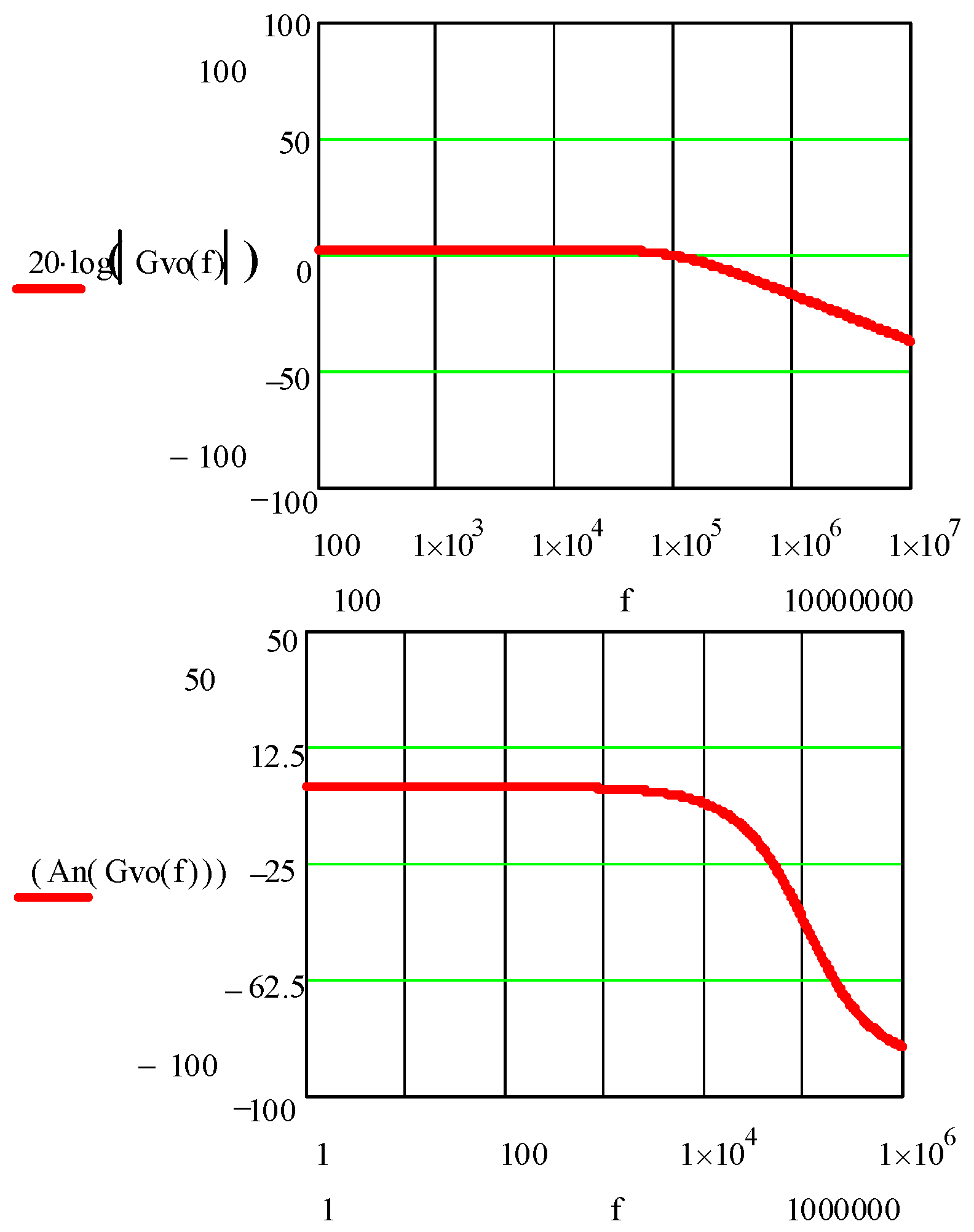
We can obtain the open-loop transfer function of the system according to Equation (15) without considering the integral regulator. This is shown in Equation (16):
The logarithmic frequency characteristic curve is shown in Figure 6. It can be seen that the cut-off frequency is 3.589 khz and the phase angle is (below ) without the regulator; thus, the system is unstable and we need to perform correction.
The integral controller is adopted and its transfer function is shown in Equation (17):
The open-loop transfer function with an integral controller is shown in Equation (18):
The correction is carried out according to the target with a phase angle margin of at 100 kHz, which is calculated by the following formula:
The solution is as shown below:
By substituting Equation (20) into Equation (18), the corrected open-loop transfer function can be obtained as shown in Equation (21):
The logarithmic frequency characteristic curve is shown in Figure 7. It shows that the expected correction effect is achieved.
It can be seen from the transfer function that the system is always stable after the I-regulator is added. From Equation (15), it can be seen that the transfer function of the system is equivalent to the first-order inertial link after adding the integral regulator. The output of the inertial link does not change in proportion to the input at the beginning. Until the end of the transition process, the output can remain proportional to the input. In order to achieve zero deviation, the system should be corrected to a type I system.Therefore, it is necessary to cascade a PI controller; the I-PI controller is used in this paper.
3.3. Zero Adjustment Based on I-PI Regulator
The control block diagram of the integral–proportional-integral controller is shown in Figure 8.
The transfer function of the I-PI controller is shown in Equation (22):
Then, calculation is performed according to the following conditions:
The solution is shown below:
According to the corresponding relationship between the PI parameters, resistance and capacitance, the calculation of the I-integrator is as follows:
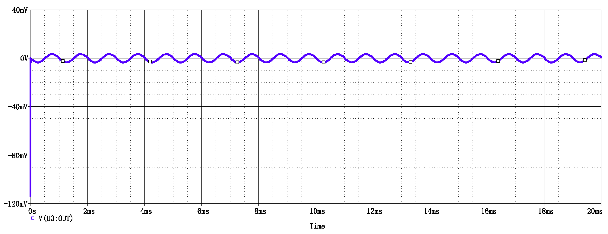
The logarithmic frequency characteristic curve is shown in Figure 9. The schematic diagram of the integral–proportional-integral regulating circuit is shown in Figure 10. The simulation waveforms are shown in Figure 11, Figure 12 and Figure 13. Compared with the steady-state error of an integral regulator, the introduction of an I-PI controller can reduce the error.
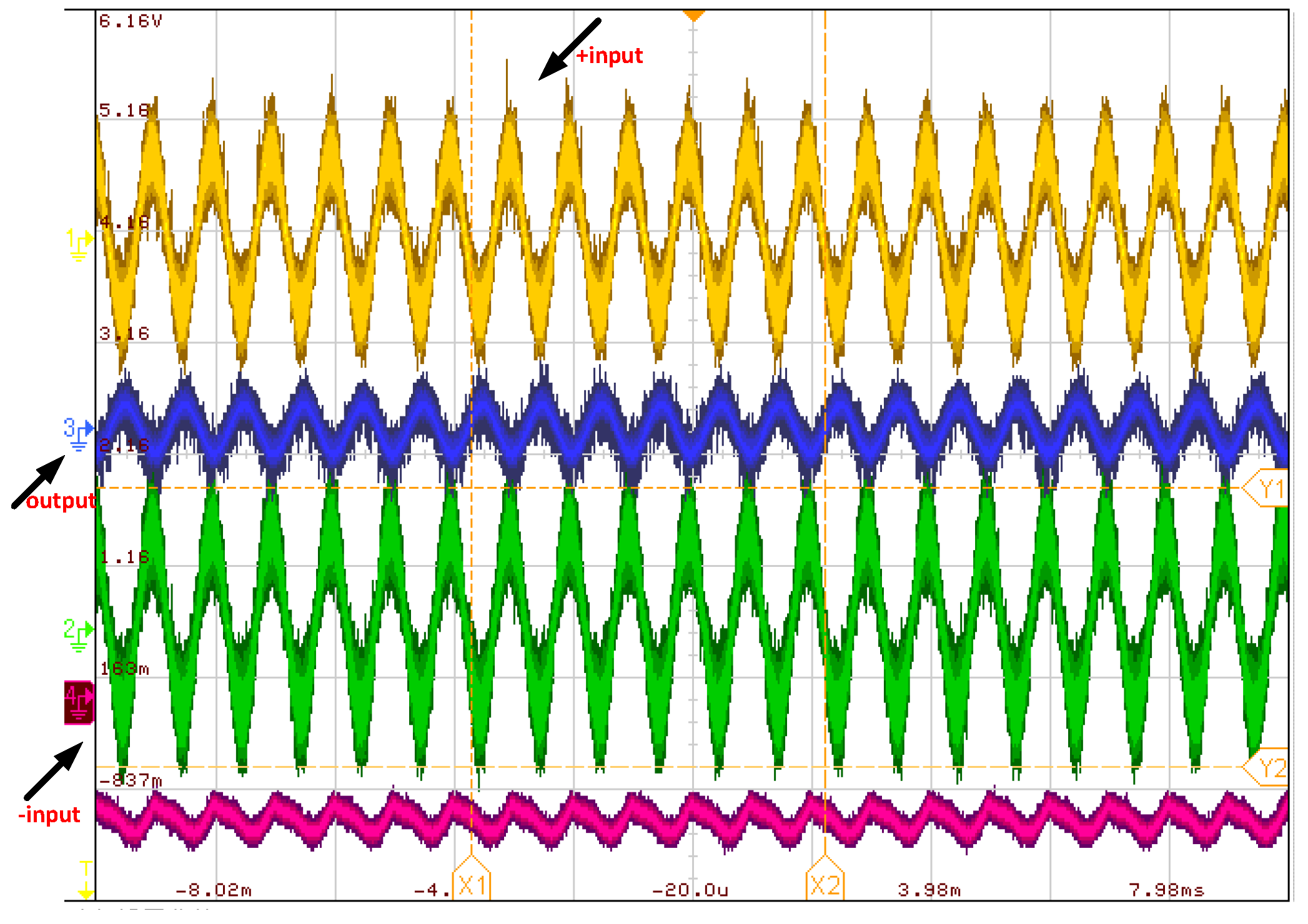
The simulation waveform of Figure 11 is the positive input voltage waveform of the amplifier, and Figure 12 is the negative input voltage waveform of the amplifier. Figure 13 is the output voltage waveform. Simulations show that the input and output waveforms coincide. The upper and lower bridge arms reach balance, and the circuit realizes the function of zero adjustment. The circuit is stable, which verifies that the control strategy is feasible and realizes the automatic zero adjustment of the measurement circuit in this paper.
4. An Implementation Method for an Inductive Proximity Sensor with an Attenuation Coefficient of 1
It can be seen from Figure 1 that when the target metal is close to the sensing surface of the detection coil, the inductance of the detection coil changes, resulting in an inductance increment . changes with the change of the approaching distance. The variable inductance increment signal is sent to the ADC converter in the FPGA circuit through the amplified electrical signal of the conditioning circuit. In the FPGA, the algorithm program mixer is used to form the proximity distance table. The proximity distance table is a table drawn according to . This proximity distance table is made according to the corresponding relationship between and . The proximity distance can be obtained by querying the table. For different target metal objects, different proximity tables are stored in the FPGA, and the distance detection of different metal targets is realized at the same sensing distance.
The corresponding relationship between and the proximity is stored in the FPGA in the form of a table, and the proximity distance is obtained by looking up the table. For different metal objects, the corresponding proximity distance table can be corrected to realize the measurement of different metal objects at the same sensing distance; that is, an inductive proximity sensor with an attenuation coefficient of 1 is realized. The FPGA circuit in Figure 1 mainly realizes the analog-to-digital conversion of . The proximity distance table is obtained by the mixer program. The proximity distance is queried according to , and then the distance signal or switch signal is output through the low-pass filter. The application of the FPGA reduces the use of some hardware circuits and helps to achieve high reliability from the inductive proximity sensor.
In order to realize an inductive proximity sensor with an attenuation coefficient of 1, it is necessary to find different tables for different metals through the FPGA in order to realize the compensation output of different metals. The overall flow chart of the FPGA look-up table method is shown in Figure 14 below.
As can be seen from Figure 14, the signal amplified by the instrument is converted to an analog-to-digital signal through the ADC chip. The digital signal is sent into the FPGA, and the digital signal is used as the address of the look-up table of the FPGA to be searched through. Different target metal objects switch different look-up tables for their signal output in order to realize the output compensation of metals with different attenuation coefficients and the on–off switching of the inductive proximity sensor for different metals at the same detection distance.
5. Experimental Results
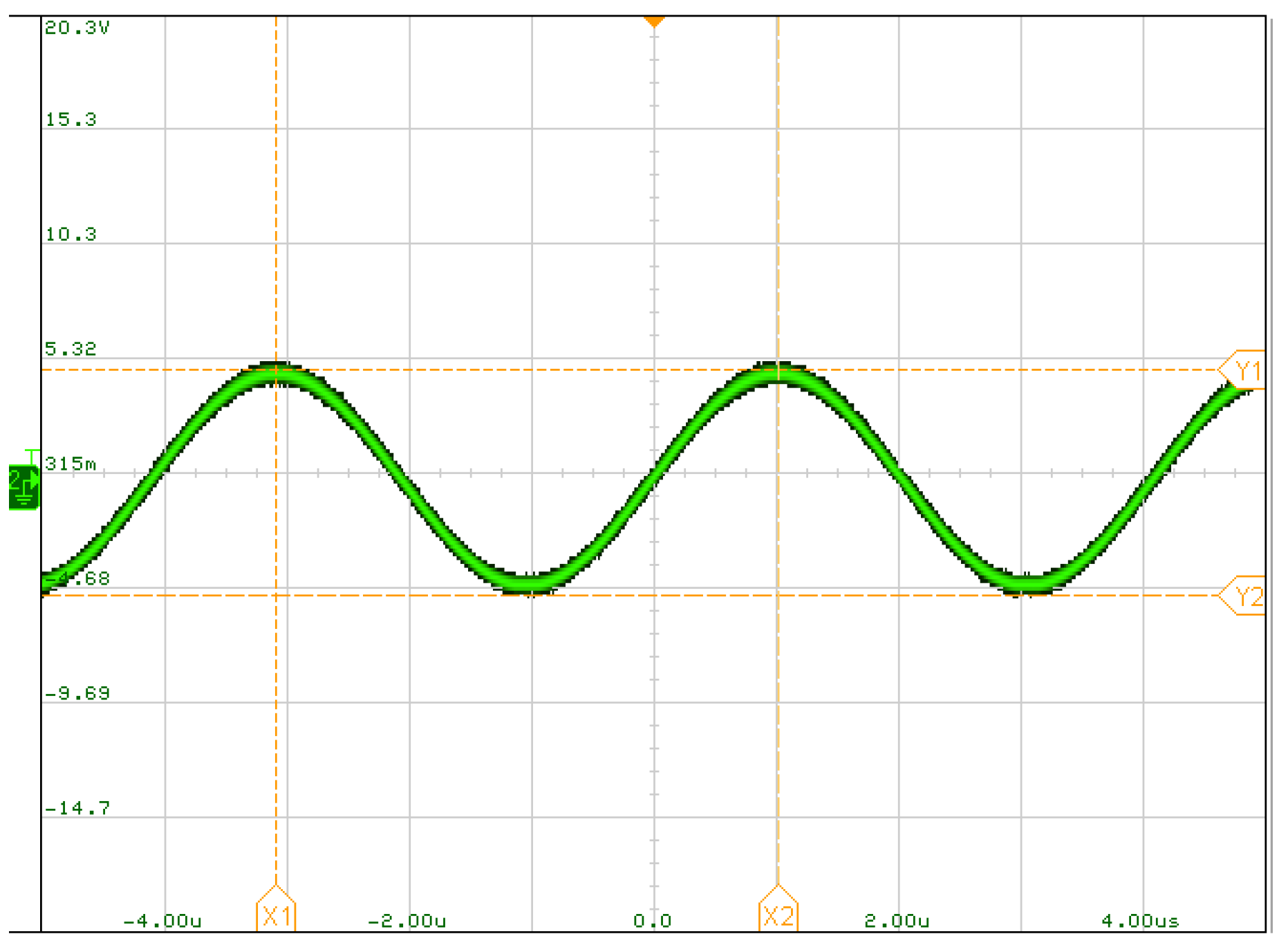
The experimental results verify the efficacy of the automatic zero adjustment technology and the inductive proximity sensor with an attenuation coefficient of 1. The FPGA chip is xc7a35tfgg484-2 from Xilinx. The ADC chip AD9280 and DAC chip AD9708 were created by the Analog Device Company. The instrument amplifier was INA101HP from Texas Instruments. The waveform of the voltage source is shown in Figure 15. The output voltage waveform after automatic zero adjustment by the I-PI controller is shown in Figure 16. The picture of the prototype is shown in Figure 17. We can see that the experimental waveforms coincide with the simulation waveforms, and the circuit achieves the function of zero adjustment.
In this paper, three kinds of metal targets are tested. Firstly, the copper is tested. The look-up table of the FPGA is switched to the copper look-up table, and the target metal that is outside the detection range is close to the sensor. At this time, the voltage of the multimeter is 0. When the copper reaches the detection distance, the multimeter changes to the supply voltage of the sensor. The distance at this time, which is the reclosing distance, is then recorded. Then, the copper is slowly moved away from the inductive proximity sensor. When the multimeter jumps to zero again, the distance at this time, which is the distance when it is disconnected, is then recorded. The above process is repeated, and three sets of data are recorded. The measurement processes for A3 steel and magnesium aluminum alloy are similar. It is only necessary to switch the FPGA look-up table to continue the experiment. Table 1 shows the test data; the unit of distance is mm. It can be seen from Table 1 that an inductive proximity sensor with an attenuation coefficient of 1 is realized; that is, different metal objects can be measured at the same distance, and we can obtain the proximity distance of the object from Table 1. The automatic zero calibration technology of the I-PI controller designed in this paper is helpful for high-precision measurement.
6. Conclusions
In this paper, a bridge differential inductance detection circuit and the FPGA are used as the electronic measurement circuit of sensors, and automatic zero adjustment technology is proposed to meet the consistency needs of product production and improve the efficiency of use of the design. Because the bridge differential inductance detection circuit can effectively suppress the common mode noise and leave an effective differential mode measurement signal, it can achieve the remote measurement of sensors. In addition, by searching for the proximity distance table corresponding to different metal objects in the FPGA, the measurement of different metal objects under the same induction distance is realized; that is, measurement with an attenuation coefficient of 1 is achieved, and the proximity of the objects can be obtained. The method studied in this paper is convenient for the production of inductive proximity sensors for the use of customers.
Author Contributions
Conceptualization, Y.Z. and Y.F.; Methodology, Y.Z.; Software and investigation, X.X. and W.Z.; Validation, Y.Z. and J.Y.; Formal analysis, Y.F. and X.G.; Writing—review and editing, S.C. and Y.F. All authors have read and agreed to the published version of the manuscript.
Funding
This work was supported in part by the equipment pre-research project under Grant 31512040201-2, in part by the National Natural Science Foundation of China under Grant 61873346, in part by the Open Project Fund of Yangzhou University Jiangdu Institute of High-end Equipment Engineering Technology under Grant YDJD201902, in part by the General competitive projects of science and technology plan in Hanjiang District of Yangzhou City under Grant HJM2019008 and in part by the Jiangsu Natural Science Foundation under Grant BK20181218.
Conflicts of Interest
The authors declare no conflict of interest.
Abbreviations
The following abbreviations are used in this manuscript:
| FPGA | Field-Programmable Gate Array |
| I-PI | Integral–Proportional-Integral |
| JFET | Junction Field-Effect Transistor |
References
- Ibrahim, M.A.; Hassan, G. A Ferrous-Selective Proximity Sensor for Industrial Internet of Things. In Proceedings of the ICC 2020-2020 IEEE International Conference on Communications (ICC), Dublin, Ireland, 7–11 June 2020. [Google Scholar]
- Bian, S.Z.; Zhou, B.; Lukowicz, P. Social distance monitor with a wearable magnetic field proximity sensor. Sensors 2020, 20, 5101. [Google Scholar]
- Matko, V.; Milanovič, M. High resolution switching mode inductance-to-frequency converter with temperature compensation. Sensors 2014, 14, 19242–19259. [Google Scholar] [CrossRef] [PubMed]
- Matko, V.; Šafarič, R. Major improvements of quartz crystal pulling sensitivity and linearity using series reactance. Sensors 2009, 9, 8263–8270. [Google Scholar] [CrossRef] [PubMed]
- Sakthivel, M.; George, B.; Jayashankar, V. A New Inductive Proximity Sensor as a Guiding Tool for Removing Metal Shrapnel During Surgery. In Proceedings of the 2013 IEEE International Instrumentation and Measurement Technology Conference (I2MTC), Minneapolis, MN, USA, 6–9 May 2013; pp. 53–57. [Google Scholar]
- Jagiella, M.; Fericean, S.; Droxler, R.; Dorneich, A. New magneto-inductive mensing principle and its implementation in sensors for industrial applications. Walter Gruyter GmbH 2004, 72, 1020–1023. [Google Scholar]
- Fericean, S.; Droxler, R. New Noncontacting Inductive Analog Proximity and Inductive Linear Displacement Sensors for Industrial Automation. IEEE Sens. J. 2007, 9, 1538–1545. [Google Scholar] [CrossRef]
- Kumar, P.; George, B. A simple signal conditioning scheme for inductive sensors. IEEE Comput. Soc. 2013, 512–515. [Google Scholar] [CrossRef]
- Chen, M.H.; Daisuke, A. Circuit Design for Commom Mode Noise Rejection in Biosignal Acquisition Based on Imbalance Cancellation of Electrode Contact Resistance. In Proceedings of the 2019 Joint International Symposium on Electromagnetic Compatibility, Sapporo and Asia-Pacific International Symposium on Electromagnetic Compatibility (EMC Sapporo/APEMC), Hokkaido, Japan, 3–7 June 2019; pp. 171–174. [Google Scholar]
- Prokopenko, N. Floating Complementary JFET Differential Stage with Increased Rejection of input Common Mode Signal and Power-Supply Noises. In Proceedings of the 2020 Moscow Workshop on Electronic and Networking Technologies (MWENT), Russia, Moscow, 11–13 March 2020. [Google Scholar]
- Yuyin, Z.; Yu, F.; Jiajun, Y. Realization of Automatic Zero Calibration of Inductive Proximity Sensor Based on Inductive Increment Detection. In Chinese Intelligent Systems Conference; Springer: Singapore, 2020; pp. 455–463. [Google Scholar]
- Matindoust, S. On-line Battery Impedance Measurement Using Oscillation Excitation. In Proceedings of the Electrical Engineering (ICEE), Mashhad, Iran, 8–10 May 2018; pp. 1729–1734. [Google Scholar]
- Simo, H.; Domguia, U.S. Analysis of Vibration of Pendulum Arm Under Bursting Oscillation Excitation; Springer: Berlin/Heidelberg, Germany, 2019. [Google Scholar]
- Strzabala, P.; Wcislik, M.; Mocan, M. Impact of the ripple output voltage of the bridge rectifier on the equivalent parameters of the AC circuit in continuous mode. In Proceedings of the 2018 Progress in Applied Electrical Engineering (PAEE), Kościelisko, Poland, 18–22 June 2018. [Google Scholar]
- Wcislik, M. Modeling of Single-Phase AC Circuit with Nonlinear Load and Power Measurement Systems. In Proceedings of the 2018 Conference on Electrotechnology: Processes, Models, Control and Computer Science (EPMCCS), Kielce, Poland, 12–14 November 2018. [Google Scholar]
- Kovshov, G.M.; Ryzhkov, I.V. On the Issue of the Increase of the Drill String Position Determination Accuracy during the Study of Temperature Influence on Primary Transducer Performance; National Mining University: Dnipro, Ukraine, 2013; pp. 78–82. [Google Scholar]
- Zheng, S.Q.; Liu, X.M. Temperature Drift Compensation for Exponential Hysteresis Characteristics of Higherature Eddy Current Displacement Sensors. IEEE Sens. J. 2019, 19, 11041–11049. [Google Scholar] [CrossRef]
- Sotner, R.; Domansky, O.; Langhammer, L. Comparison of simple design methods for voltage controllable resistance. In Proceedings of the 2020 30th International Conference Radioelektronika (RADIOELEKTRONIKA), Bratislava, Slovakia, 15–16 April 2018. [Google Scholar]
- Bilik, V.; Krajcovic, F. Coaxial 2.45-GHz high power impedance matching device. In Proceeding of the 13th International Conference on Microwave and Radio Frequency Heating; Editions Cepadues: Toulouse, France, 2011; pp. 129–132. [Google Scholar]
- Masuda, S.; Hirose, T.; Akihara, Y. Impedance matching in magnetic-coupling-resonance wireless power transfer for small implantable devices. In Proceedings of the 2017 IEEE Wireless Power Transfer Conference (WPTC), Taipei, Taiwan, 10–12 May 2017. [Google Scholar]
- King, K.M. Railway Control Safety Systems as a Closed Loop Negative Feedback Control System; Institution of Engineering and Technology: London, UK, 2011. [Google Scholar]
- Dilib, F.A.; Jackson, M.D.; Mojaddam, Z.A. Closed-loop feedback control in intelligent wells: Application to a heterogeneous, thus oil-rim reservoir in the North sea. SPE Reserv. Eval. Eng. 2015, 18, 69–83. [Google Scholar] [CrossRef]
- Maide, B.; Arturo, B.; Carlo, F.; Luigi, F.; Mattia, F. Control of imperfect dynamical systems. Nonlinear Dyn. 2019, 98, 2989–2999. [Google Scholar]
- Hussien, M.G. Mathematical Analysis of the Small Signal Model for Voltage-Source Inverter in SPMSM Drive Systems. In Proceedings of the 2019 21st International Middle East Power Systems Conference (MEPCON), Cairo, Egypt, 17–19 December 2019; pp. 540–549. [Google Scholar]
Figure 1.
Schematic diagram of an inductive proximity sensor. FPGA: field-programmable gate array. ADC: analog to digital conversion. LPF: low pass filtering.
Figure 1.
Schematic diagram of an inductive proximity sensor. FPGA: field-programmable gate array. ADC: analog to digital conversion. LPF: low pass filtering.

Figure 2.
Schematic diagram of bridge differential inductance detection circuit.

Figure 3.
Schematic diagram of general impedance converter.

Figure 4.
Circuit schematic diagram of bias inductance Lr.

Figure 5.
Block diagram of I controller.

Figure 6.
Open loop Bode diagram without regulator.

Figure 7.
Open loop Bode diagram with I regulator.

Figure 8.
Control block diagram of the integral–proportional-integral (I-PI) controller.

Figure 9.
Open loop Bode diagram with I-PI regulator.

Figure 10.
Integral–proportional-integral regulating circuit.

Figure 11.
Positive input voltage waveform of amplifier.

Figure 12.
Negative input voltage waveform of amplifier.

Figure 13.
Output voltage waveform of amplifier.

Figure 14.
Schematic diagram of the inductive proximity sensor with an attenuation coefficient of 1.
Figure 14.
Schematic diagram of the inductive proximity sensor with an attenuation coefficient of 1.

Figure 15.
Excitation source waveform.

Figure 16.
Experimental waveform.

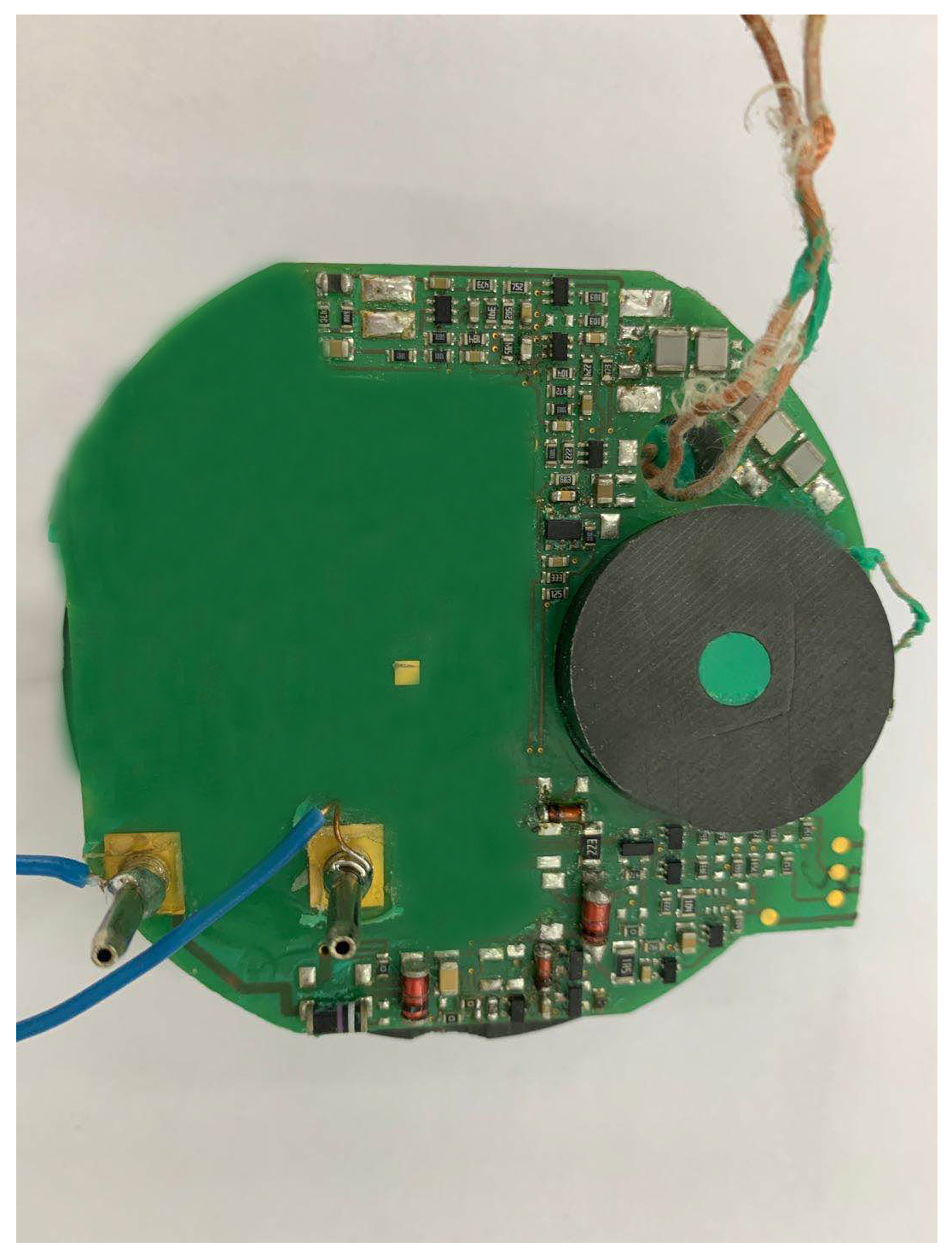
Figure 17.
Picture of the engineering prototype.


Table 1.
Test data sheet of different metals (unit: mm).
| Target | Effective Distance Error | Available Action Range | Repeatability Accuracy | Distance at Disconnection | Reclose Distance | Return Error |
|---|---|---|---|---|---|---|
| Copper | 0.9716 | 36.45–44.55 | 4.05 | 42.2000 | 43.0729 | 0.8729 |
| 42.4756 | 43.1716 | 0.6960 | ||||
| 42.3743 | 43.0712 | 0.6969 | ||||
| A3 steel | 0.7978 | 36.45–44.55 | 4.05 | 44.4238 | 45.1153 | 0.6915 |
| 44.4265 | 45.2206 | 0.7941 | ||||
| 44.5273 | 45.2216 | 0.6943 | ||||
| Alumin | 0.6948 | 36.45–44.55 | 4.05 | 41.9885 | 42.6791 | 0.6906 |
| 41.9903 | 42.6815 | 0.6912 | ||||
| 41.9917 | 42.6833 | 0.6916 |
Publisher’s Note: MDPI stays neutral with regard to jurisdictional claims in published maps and institutional affiliations. |
© 2020 by the authors. Licensee MDPI, Basel, Switzerland. This article is an open access article distributed under the terms and conditions of the Creative Commons Attribution (CC BY) license (http://creativecommons.org/licenses/by/4.0/).
Share and Cite
MDPI and ACS Style
Zhao, Y.; Fang, Y.; Yang, J.; Zhang, W.; Ge, X.; Cao, S.; Xia, X. An Implementation Method for an Inductive Proximity Sensor with an Attenuation Coefficient of 1. Energies 2020, 13, 6482. https://doi.org/10.3390/en13246482
AMA Style
Zhao Y, Fang Y, Yang J, Zhang W, Ge X, Cao S, Xia X. An Implementation Method for an Inductive Proximity Sensor with an Attenuation Coefficient of 1. Energies. 2020; 13(24):6482. https://doi.org/10.3390/en13246482
Chicago/Turabian StyleZhao, Yuyin, Yu Fang, Jiajun Yang, Weixuan Zhang, Xiaoxing Ge, Songyin Cao, and Xiaonan Xia. 2020. "An Implementation Method for an Inductive Proximity Sensor with an Attenuation Coefficient of 1" Energies 13, no. 24: 6482. https://doi.org/10.3390/en13246482
Note that from the first issue of 2016, this journal uses article numbers instead of page numbers. See further details here.