Conflict Management for Target Recognition Based on PPT Entropy and Entropy Distance

Abstract

Conflicting evidence affects the final target recognition results. Thus, managing conflicting evidence efficiently can help to improve the belief degree of the true target. In current research, the existing approaches based on belief entropy use belief entropy itself to measure evidence conflict. However, it is not convincing to characterize the evidence conflict only through belief entropy itself. To solve this problem, we comprehensively consider the influences of the belief entropy itself and mutual belief entropy on conflict measurement, and propose a novel approach based on an improved belief entropy and entropy distance. The improved belief entropy based on pignistic probability transformation function is named pignistic probability transformation (PPT) entropy that measures the conflict between evidences from the perspective of self-belief entropy. Compared with the state-of-the-art belief entropy, it can measure the uncertainty of evidence more accurately, and make full use of the intersection information of evidence to estimate the degree of evidence conflict more reasonably. Entropy distance is a new distance measurement method and is used to measure the conflict between evidences from the perspective of mutual belief entropy. Two measures are mutually complementary in a sense. The results of numerical examples and target recognition applications demonstrate that our proposed approach has a faster convergence speed, and a higher belief degree of the true target compared with the existing methods.

1. Introduction

Information is affected by various subjective factors and objective environment, and there is some uncertainty. How to measure uncertainty has become an open issue. Some theoretical tools have been proposed, including probability theory [1], fuzzy set theory [2,3], D-numbers [4,5], Z-numbers [6,7], rough set theory [8,9], Dempster-Shafer (D-S) evidence theory [10,11], fractal theory [12,13], etc. D-S evidence theory is one of the most effective tools among them. It not only allocates belief to the power set of propositions [14], but also has the acceptance of an incomplete model without prior probabilities [15]. For this reason, D-S evidence theory has been widely applied in risk analysis [16,17], uncertainty [18], fault diagnosis [19], decision making [20], and so on.

However, a counterintuitive result is generated when there is a high degree of conflict between the evidences. To address this issue, researchers have proposed a variety of improved methods which can be divided into modifying Dempster’s combination rule [21,22,23] and modifying the original evidence. For the first class, Smets et al. think that the conflict should be assigned to empty set [21]. Lefevre et al. propose a modified method which proportionally distributed the conflict information to the focal element sets [22]. Whereas, the flaw of the modification of Dempster’s combination rule is that the good performance is destructed, like commutativity and associativity. Therefore, many researchers are inclined to modify the original evidence. For the second class, the initial evidences are modified by corresponding weights and rational combined results can be achieved by using the classical Dempster’s rule. Therefore, the most commonly used method is the weighted evidence combination. Jiang et al.’s method obtains the weight of evidence by jointly using the distance of evidence and Deng entropy [24]. Tao et al. propose a modified average method to combine conflicting evidence based on belief entropy and induced ordered weighted averaging operator [25]. Li et al. define a new discount coefficient to modify the original evidence based on Belief Entropy and Negation [26]. In contrast, some existing methods [27,28,29] are based on belief entropy and use belief entropy itself to measure evidence conflict. Obviously, it is not convincing to characterize the evidence conflict only through belief entropy itself. Especially when the belief entropy of conflict evidence and normal evidence is close, the conflict evidence will point to a weight almost equal to that of normal evidence, and conflicts are not handled effectively.

To overcome the shortcomings of the methods, we propose a novel method based on an improved entropy and entropy distance, taking into account both the impacts of self-belief entropy and mutual belief entropy on conflict management. The improved belief entropy is used to quantify the uncertainty of the evidence, so as to measure the degree of conflict from a global perspective. PPT entropy introduces pignistic probability transformation function into Yan et al.’s entropy [27]. Compared with the state-of-the-art belief entropy [27,30,31,32,33,34], it can measure the uncertainty of evidence more accurately, and make full use of the intersection information of evidence to better estimate the degree of evidence conflict. Given the good performance of PPT entropy, this paper chooses it to measure the uncertainty of body of evidence (BOE). Entropy distance describes the entropy difference between evidence, so as to measure the degree of conflict from a local perspective. These two measures are mutually complementary in a sense.

The proposed method deals with conflicting evidence in a more comprehensive way, so that the conflict measurement could be more accurate and reasonable. No matter whether the belief entropy of conflict evidence and normal evidence is equal, close or a large difference, it can still identify conflict evidence and assign a smaller weight to conflict evidence. Not only the drawbacks of existing methods are overcome, but also it has a better convergence performance. Two numerical examples in experiments are illustrated that the novel method is feasible and superior in dealing with the conflicting evidence, where the belief degree of the correct hypothesis has 3.8% and 1.6% increase compared to existing methods, respectively. Furthermore, the belief degree of the true target increases to 98.8% in target recognition application. In this research, the support degree of BOE is a fractional form in which PPT entropy is treated as a numerator and the sum of entropy distances as a denominator. The greater the conflict between the evidences, the greater the entropy distance and the smaller the weight of conflicting evidence.

In this paper, two contributions can be summarized as follows:

• We propose PPT entropy based on pignistic probability transformation function. It fully considers the influence of the intersection between propositions on uncertainty and makes the uncertainty measurement of evidence more accurate and range wider.
• A novel method for conflict management is presented based on PPT entropy and entropy distance. It measures conflict between evidences from the perspective of belief entropy itself and mutual belief entropy. Not only it has a better convergence performance, but also the higher belief value of the correct hypothesis and true target is obtained.

To facilitate our discussion, Section 2 introduces some basic concepts. In Section 3, we propose PPT entropy and entropy distance. The property and requirements of behaviour of PPT entropy are discussed, and some examples are provided to illustrate the validity of our proposed belief entropy. Based on that, a novel method of conflict management is presented. In Section 4, an application in target recognition is shown to verify the effectiveness of our proposed method. Section 5 is the conclusion.

2. Preliminaries

In this section, some preliminaries are briefly introduced, including D-S evidence theory, several typical belief entropies and pignistic probability transform, for the purpose of understanding the descriptions in the rest of this paper.

2.1. D-S Evidence Theory

Suppose $\mathsf{\Theta }$ is a set of mutually exclusive and exhaustive elements $F_i$$(i=1,2,3,4,\dots ,$$N),$ and it can be defined as [32]

$$\mathsf{\Theta }=\left\{F_1,F_2,F_3,F_4,\dots ,F_N\right\}$$

(1)

where $\mathsf{\Theta }$ is called the frame of discernment (FOD), and $F_i$ is named single-element proposition or subset. We define $2^{\mathsf{\Theta }}$ as a power set which contains $2^N$ elements and can be described as

$$\begin{array}{c}\hfill 2^{\mathsf{\Theta }}=\left\{⌀,F_1,F_2,\dots ,F_N,\left\{F_1,F_2\right\},\left\{F_1,F_3\right\},\dots ,\mathsf{\Theta }\right\}\end{array}$$

(2)

where ⌀ is an empty set in Equation (2), and the basic probability assignment (BPA) function m is defined as a mapping of the power set $2^{\mathsf{\Theta }}$ to [0,1].

$$m:2^{\mathsf{\Theta }}\to [0,1]$$

which satisfies

$$\begin{array}{ccccc}& & \hfill m(⌀)& =0\hfill & \\ & & \hfill 0\le m\left(A\right)& \le 1\hfill & \\ & & \hfill \sum _{A\subseteq \mathsf{\Theta }}m\left(A\right)& =1\hfill \end{array}$$

where mass function $m\left(A\right)$ represents the probability of support to $A,$ and A is called focal element, proposition or subset. This paper researches classical D-S evidence theory, so the mass function $m\left(\varphi \right)$ is equal to 0.

The belief function $Bel\left(A\right)$ can be defined as [31]

$$Bel\left(A\right)=\sum _{B\subseteq A}m\left(B\right)$$

(3)

where $Bel\left(A\right)$ represents the total belief to the proposition A. In D-S evidence theory, two BPAs can be combined with Dempster’ s rule of combination, defined as follows [35]:

$$m\left(A\right)=\left(m_1\oplus m_2\right)\left(A\right)=\frac{1}{1-K}\sum _{B\cap C=A}{m}_1\left(B\right)m_2\left(C\right)$$

(4)

in which

$$K=\sum _{B\cap C=⌀}{m}_1\left(B\right)m_2\left(C\right)$$

(5)

where ⊕ represents Dempster’s combination rule. K is called conflict coefficient, and its scope is [0, 1]. The bigger K is, the more conflict between two evidences is.

2.2. Entropy

Several typical belief entropies are briefly introduced.

2.2.1. Shannon Entropy

Shannon entropy is an uncertain measure of information volume and is denoted by [27]:

$$H=-\sum _{i=1}^N{p}_i{log}_2{p}_i$$

(6)

where N is the number of basic states in the system, $p_i$ is the probability of state i and it satisfies ${\sum }_{i=1}^N{p}_i=1$. The larger the Shannon entropy H is, the higher the uncertainty degree is.

2.2.2. Deng Entropy

Shannon entropy has a great contribution to the measurement of uncertainty, but it has some limitations when there is the BPA. Because it measures uncertainty based on probability. In order to solve this problem, Deng proposes Deng entropy in the framework of D-S evidence theory. It is a generalization of Shannon entropy and is defined as [30]:

$$E_d\left(m\right)=\sum _{A\subseteq \mathsf{\Theta }}m\left(A\right){log}_2(2^{\left|A\right|}-1)-\sum _{A\subseteq \mathsf{\Theta }}m\left(A\right){log}_{2}m\left(A\right)$$

(7)

where $\left|A\right|$ is the cardinality of the proposition A, that is, the total number of single-element subsets contained in the proposition A.

2.2.3. Zhou et al.’s Entropy

Zhou et al.’s belief entropy considers the influence of the scale of BOE on uncertainty and is denoted by [31]:

$$E_{Md}\left(m\right)=\sum _{A\subseteq \mathsf{\Theta }}m\left(A\right){log}_2\frac{2^{\left|A\right|}-1}{e^{\frac{\left|A\right|-1}{\left|S\right|}}}-\sum _{A\subseteq \mathsf{\Theta }}m\left(A\right){log}_{2}m\left(A\right)$$

(8)

where $\left|S\right|$ is the cardinality of the $\mathsf{\Theta }$, that is, the total number of single-element subsets contained in the FOD.

2.2.4. Yan et al.’s Entropy

Yan et al.’s belief entropy uses the belief function to extend method of measuring uncertain and is an improved method based on Zhou’s belief entropy as follows [27]:

$$\begin{array}{c}\hfill H_n\left(m\right)=\sum _{A\subseteq \mathsf{\Theta }}m\left(A\right){log}_2\frac{2^{\left|A\right|}-1}{e^{\frac{\left|A\right|-1}{\left|S\right|}}}-\sum _{A\subseteq \mathsf{\Theta }}m\left(A\right){log}_2\frac{m\left(A\right)+Bel\left(A\right)}{2}\end{array}$$

(9)

2.3. Pignistic Probability Transform

Pignistic probability transform is defined as follows [36],

$${BetP}_m\left(A\right)=\sum _{B\subseteq \mathsf{\Theta }}\frac{|A\cap B|}{\left|B\right|}\frac{m\left(B\right)}{1-m(⌀)}$$

(10)

where $|A\cap B|$ is the cardinality of the intersection of A and B. The mass function $m(⌀)$ is equal to 0 in a closed world (i.e., in classical D-S evidence theory). So it can be simplified to the following form.

$$Bet{P}_m\left(A\right)=\sum _{B\subseteq \mathsf{\Theta }}\frac{|A\cap B|}{\left|B\right|}m\left(B\right)$$

(11)

3. Proposed Method for Conflict Management

In evidence theory, a counterintuitive result is generated when combining the highly conflicting evidence. To address this problem, it is necessary to assign weights to the evidence reasonably. Some existing approaches put forward to use self-belief entropy to determine the weights of evidence. However, it fails to identify the conflicting evidence when the belief entropy of conflicting evidence and normal evidence is equal or close. In this paper, through comprehensively consider the influence of self-belief entropy and mutual belief entropy on the conflict, we proposed a novel method based on PPT entropy and entropy distance. In the following section, we first propose PPT entropy, and then entropy distance. Based on that, a novel method of conflict management is presented.

3.1. PPT Entropy

In D-S evidence theory, pignistic probability transform is described as allocating the belief to each proposition equally [37]. The essence is the influence of the intersection between propositions on proposition’s belief degree. In this literature, we introduce pignistic probability transformation function to extend the method of uncertainty measurement. The proposed belief entropy is denoted as follows:

$$H_p\left(m\right)=-\sum _{A\subseteq \mathsf{\Theta }}m\left(A\right){log}_2\frac{m\left(A\right)+Bet{P}_m\left(A\right)}{2\left(2^{\left|A\right|}-1\right)}{e}^{\frac{\left|A\right|-1}{\left|S\right|}}$$

(12)

where ${BetP}_m\left(A\right)$ is pignistic probability transform function as shown in Equation (11). The proposed belief entropy is named PPT entropy. We can infer from the Equation (12) that the PPT entropy is degenerated into Zhou et al.’s belief entropy when multi-element propositions are not in intersection. Furthermore, it is degenerated into Shannon entropy when there is only single-element propositions.

3.2. The Properties of PPT Entropy

3.2.1. Probability Consistency

When m is a Bayesian BPA, PPT entropy must be degenerated into Shannon entropy.

Proof. 

When $\left|A\right|\to 1$, it is ${BetP}_m\left(A\right)=m\left(A\right)$.

Then, we can further get:

$$\begin{array}{cc}\hfill H_p\left(m\right)& {\displaystyle =-\sum _{A\subseteq \mathsf{\Theta }}m\left(A\right){log}_2\frac{m\left(A\right)+m\left(A\right)}{2\left(2^{\left|A\right|}-1\right)}{e}^{\frac{\left|A\right|-1}{\left|S\right|}}}\hfill \\ \hfill & =-\sum _{A\subseteq \mathsf{\Theta }}m\left(A\right){log}_{2}m\left(A\right)\hfill \end{array}$$

Hence, the probability consistency holds.  □

3.2.2. Set Consistency

Suppose that the PPT entropy satisfies the property of set consistency when exists a set A such that $m\left(A\right)=1$, which means that it must satisfy the equation:

$$\begin{array}{c}{H}_p\left(m\right)={log}_2\left(\right|A\left|\right)\hfill \end{array}$$

Proof. 

Suppose that the $\mathrm{FOD}$ is $\mathsf{\Theta }=\left\{{\theta }_1,{\theta }_2,{\theta }_3\right\}$ and the BPA is $m\left(A\right)=1,\forall A=\mathsf{\Theta }$ (i.e., $\left|A\right|=\left|\mathsf{\Theta }\right|=3)$.

We can get

$$\begin{array}{ccccc}& & \hfill H_p\left(m\right)& =-1\times {log}_2\frac{1+\frac{3}{3}\times 1}{2\left(2^3-1\right)}{e}^{\frac{3-1}{3}}={log}_{2}3.6\hfill & \\ & & \hfill {log}_2\left(\right|A\left|\right)& ={log}_{2}3\hfill \end{array}$$

obviously

$$H_p\left(m\right)\ne {log}_2\left(\right|A\left|\right)$$

Hence, the set consistency does not hold. □

3.2.3. Range

Mathematically, the value range of PPT entropy is $[0,+\infty )$.

First, PPT entropy is always non-negative.

Proof. 

We know

$$\begin{array}{c}0\le m\left(A\right)\le 1\hfill \\ {\displaystyle 0\le \frac{m\left(A\right)+Bet{P}_m\left(A\right)}{2}\le 1}\hfill \\ {\displaystyle 0\le e^{\frac{\left|A\right|-1}{\left|S\right|}}\le \mathrm{e}\le 3}\hfill \end{array}$$

if $\left|\mathrm{A}\right|=1$

$$H_p\left(m\right)=-\sum _{A\subseteq \mathsf{\Theta }}m\left(A\right){log}_{2}m\left(A\right)\ge 0$$

if $\left|\mathrm{A}\right|\ge 2$

$$\begin{array}{cc}\hfill 2^{\left|A\right|}-1& \ge 3\hfill \\ \hfill e^{\frac{\left|A\right|-1}{\left|S\right|}}/\left(2^{\left|A\right|}-1\right)& \le 1\hfill \\ \hfill H_p\left(m\right)& \ge 0\hfill \end{array}$$

thus:

$$H_p\left(m\right)\ge 0$$

Second, the maximum value of PPT entropy is infinite. □

The proposition A and the FOD $\mathsf{\Theta }$ consist of at least one single-element subset and there is no superior limit, thus the range of $\left|A\right|$ and $\left|S\right|$ are [1,+∞). Moreover, the range of $m\left(A\right)$ and $Bet{P}_m\left(A\right)$ are $[0,1]$. Obviously, the maximum value of PPT entropy is infinite according to the Equation (12).

Finally, we can conclude that the value range of PPT entropy is $[0,+\infty )$.

3.2.4. Additivity

Suppose that the PPT entropy satisfies the additivity, which means that it satisfies the equation:

$$H_p\left(m\left({\mathsf{\Theta }}_1\times {\mathsf{\Theta }}_2\right))=H_p\left(m_{{\mathsf{\Theta }}_1}\right)+H_p\left(m_{{\mathsf{\Theta }}_2}\right)\right.$$

where ${\mathsf{\Theta }}_1\times {\mathsf{\Theta }}_2$ is the product space of the sets ${\mathsf{\Theta }}_1$ and ${\mathsf{\Theta }}_2$ and m is a $BPA$ on ${\mathsf{\Theta }}_1\times {\mathsf{\Theta }}_2.$ It also need to satisfy $m(A\times B)=$$m\left(A\right)m\left(B\right)$ with $A\subseteq {\mathsf{\Theta }}_1,B\subseteq {\mathsf{\Theta }}_2$

Proof. 

Assume $X\times Y$ is the product space of two FODs $X=\left\{x_1,x_2,x_3\right\},Y=\left\{y_1,y_2\right\}.$ The marginal BPAs on $X\times Y$ are the following ones:

$$\begin{array}{cc}\hfill & m_1:m_1\left(x_1,x_2\right)=0.5,m_1\left(x_3\right)=0.2,m_1\left(X\right)=0.3\hfill \\ \hfill & m_2:m_2\left(Y\right)=1\hfill \\ \hfill & m:m\left(z_{11},z_{12},z_{21},z_{22}\right)=0.5,m\left(z_{31},z_{32}\right)=0.2,m(X\times Y)=0.3\hfill \end{array}$$

where $z_{ij}=\left(x_i,y_j\right),$ we can get

$$\begin{array}{cc}\hfill H_p\left(m_1\right)+H_p\left(m_2\right)& =2.061+0.863=2.924\hfill \\ \hfill H_p\left(m\right)& =4.249\hfill \end{array}$$

obviously

$$H_p\left(m\right)>H_p\left(m_1\right)+H_p\left(m_2\right)$$

Therefore, the additivity does not hold. □

3.2.5. Subadditivity

If the PPT entropy satisfies the following conditions:

$$H_p\left(m\left({\mathsf{\Theta }}_1\times {\mathsf{\Theta }}_2\right)\right)\le H_p\left(m_{{\mathsf{\Theta }}_1}\right)+H_p\left(m_{{\mathsf{\Theta }}_2}\right)$$

where m is a BPA on the space ${\mathsf{\Theta }}_1\times {\mathsf{\Theta }}_2,m\left({\mathsf{\Theta }}_1\right)$ and $m\left({\mathsf{\Theta }}_2\right)$ are marginal BPAs on ${\mathsf{\Theta }}_1$ and ${\mathsf{\Theta }}_2$, then it is said that PPT entropy satisfies the subadditivity.

According to the property of additivity, we have got $H_p\left(m\right)>H_p\left(m_1\right)+H_p\left(m_2\right).$

Therefore, the subadditivity does not hold.

3.2.6. Monotonicity

Given two FODs ${\mathsf{\Theta }}_1$ and ${\mathsf{\Theta }}_2,$ if $\left|{\mathsf{\Theta }}_1\right|\le \left|{\mathsf{\Theta }}_2\right|$, there exists $H_p\left({\mathsf{\Theta }}_1\right)\le H_p\left({\mathsf{\Theta }}_2\right)$, then it is said that PPT entropy satisfies the monotonicity.

Proof. 

When $\left|{\mathsf{\Theta }}_1\right|\le \left|{\mathsf{\Theta }}_2\right|$

$$\begin{array}{cc}\hfill \left|S_1\right|& \le \left|S_2\right|\hfill \\ \hfill e^{\frac{\left|A\right|-1}{\left|S_1\right|}}& \ge e^{\frac{\left|A\right|-1}{\left|S_2\right|}}\hfill \end{array}$$

we can get

$$H_p\left({\mathsf{\Theta }}_1\right)\le H_p\left({\mathsf{\Theta }}_2\right)$$

Therefore, the monotonicity holds. □

To analyze the proposed entropy,

Table 1. The properties of different entropies.

Entropy	Probability Consistency	Set Consistency	Maximum Entropy	Additivity	Subadditivity	Monotonicity
Pal et al. [38]	Yes	Yes	No	Yes	No	Yes
Jousselme et al. [39]	Yes	Yes	No	Yes	No	Yes
Deng [30]	Yes	No	No	No	No	Yes
Zhou et al. [31]	Yes	No	No	No	No	Yes
Yan et al. [27]	Yes	No	No	No	No	Yes
Proposed entropy	Yes	No	No	No	No	Yes

shows the properties of different entropies. Although the PPT entropy satisfies the probability consistency and monotonicity which can be considered as two important properties for uncertainty measure, it does not satisfy set consistency, additivity and subadditivity, which will bring some challenges to the extension of the uncertainty measure on more general theories. In addition, its scope of application will be limited to a certain extent.

3.3. Requirements of Behaviour for PPT Entropy

The requirements of behaviour (RB) for uncertainty measures suggested by Abellan and Masegosa [40] could be expressed in the following way:

RB1: The calculation of uncertainty measure should be simple.

RB2: The uncertainty measure should reflect the uncertainty of conflict and non-specificity co-existing in the D-S evidence theory.

RB3: The uncertainty measure should be sensitive to change of the BPA.

RB4: The extension of the uncertainty measure in the D-S evidence theory on more general theories must be possible.

In the next section, we will discuss the above requirements of behaviour for PPT entropy.

3.3.1. Low Computing Complexity

The PPT entropy has a relatively simple calculation and it is only necessary to obtain the pignistic probability transform function $Bet{P}_m\left(A\right)$ according to the given BPA. When the mass assignments are only transferred to single-element propositions, the PPT entropy is degenerated into Shannon entropy and the calculation is simpler.

3.3.2. Concealment of Conflict and Non-Specificity

A simple transformation of Equation (12) is as follows.

$$\begin{array}{cc}\hfill H_p\left(m\right)& =\sum _{A\subseteq \mathsf{\Theta }}m\left(A\right){log}_2\left(2\left(2^{\left|A\right|}-1\right)e^{\frac{1-\left|A\right|}{\left|S\right|}}\right)-\sum _{A\subseteq \mathsf{\Theta }}m\left(A\right){log}_2\left(m\left(A\right)+\sum _{B\subseteq \mathsf{\Theta }}\frac{|A\cap B|}{\left|B\right|}m\left(B\right)\right)\hfill \end{array}$$

where the last term of the above equation ${\sum }_{A\subseteq \mathsf{\Theta }}m\left(A\right){log}_2\left(m\left(A\right)+{\sum }_{B\subseteq \mathsf{\Theta }}\frac{|A\cap B|}{\left|B\right|}m\left(B\right)\right)$ can not be further transformed into a form similar to Shannon entropy, so that it does not measure the uncertainty of conflict. Similarly, the first term ${\sum }_{A\subseteq \mathsf{\Theta }}m\left(A\right){log}_2\left(2\left(2^{\left|A\right|}-1\right)e^{\frac{1-\left|A\right|}{\left|S\right|}}\right)$ can not be further transformed into a form similar to I [40] and couldn’t measure the uncertainty of non-specificity. In other words, PPT entropy couldn’t be converted into a linear combination of $S^{*}$ and I. Here, function $S^{*}$ is used as a conflict measure and function I as a non-specificity measure. I has the following expression:

$$I\left(m\right)=\sum _{A\subseteq \mathsf{\Theta }}m\left(A\right)ln\left|A\right|$$

Therefore, PPT entropy has no clear separation between conflict and non-specificity.

3.3.3. Sensitivity to Changes in Evidence

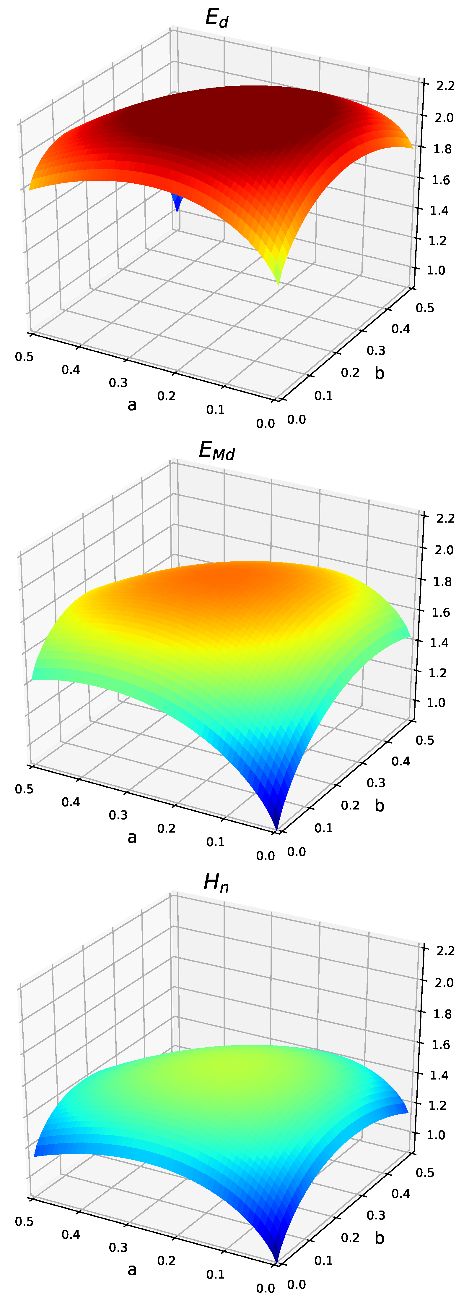
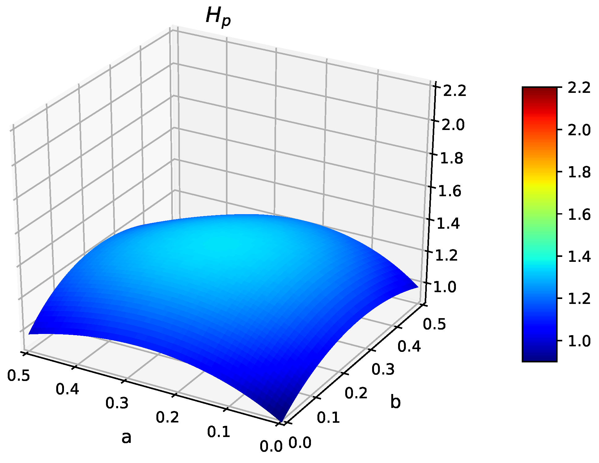
The PPT entropy is sensitive to change of the BPA. A detailed analysis is presented in Example 5. The value of $H_p$ could change with the change of the BPA as shown in Figure 1.

3.3.4. Extension on More General Theories

Currently, the belief entropy based on Deng entropy in the D-S evidence theory framework are limited to the closed world where the FOD is assumed to be complete. Tang et al. propose the nonzero mass function of the empty set (i.e., $m(⌀)\ne 0$) which extends belief entropy theory to the open world [34]. The calculation of $H_p$ contains the $m(⌀)$ as shown in Equation (10), so the extension of PPT entropy on more general belief entropy theory is possible when there is $m(⌀)\ne 0$. However, there are two key problems when it is extended on more general belief entropy theory. On the one hand, the PPT entropy only satisfies the property of probability consistency with respect to Klir’s five requirements, which is a huge challenge to extend belief entropy theory. On the other hand, the PPT entropy will be meaningless when it is $m(⌀)=1$.

3.4. Examples

In this section, two counter examples and eight numerical examples (Examples 5–9 from Yang and Han’s paper [41]) are used to illustrate the validity of PPT entropy and compare it with other uncertainty measures including Deng entropy, Zhou et.al’s belief entropy and Yan et.al’s belief entropy.

3.4.1. Counter-Example 1

Example 1.

Suppose that the FOD is $\mathsf{\Theta }=\{A,B,C,D\}$ and there is only intersection relationship between propositions in BOEs.

$$S_1:m_1(A,B)=0.3m_1(B,C)=0.3m_1(B,D)=0.4$$

$$S_2:m_2(A,B)=0.3m_2(C,D)=0.3m_2(B,D)=0.4$$

$$S_3:m_3(A,B)=0.3m_3(A,C)=0.3m_3(B,D)=0.4$$

The belief entropy is calculated with Deng entropy as follows:

$$\begin{array}{cc}\hfill E_d\left(m_1\right)& =-2\times 0.3{log}_2\frac{0.3}{2^2-1}-0.4{log}_2\frac{0.4}{2^2-1}=3.156\hfill \\ \hfill E_d\left(m_2\right)& =-2\times 0.3{log}_2\frac{0.3}{2^2-1}-0.4{log}_2\frac{0.4}{2^2-1}=3.156\hfill \\ \hfill E_d\left(m_3\right)& =-2\times 0.3{log}_2\frac{0.3}{2^2-1}-0.4{log}_2\frac{0.4}{2^2-1}=3.156\hfill \end{array}$$

The belief entropy is calculated with Zhou et al.’s belief entropy as follows:

$$\begin{array}{cc}\hfill E_{Md}\left(m_1\right)& =-2\times 0.3{log}_2\left(\frac{0.3}{2^2-1}{e}^{\frac{2-1}{4}}\right)-0.4{log}_2\left(\frac{0.4}{2^2-1}{e}^{\frac{2-1}{4}}\right)=2.795\hfill \\ \hfill E_{Md}\left(m_2\right)& =-2\times 0.3{log}_2\left(\frac{0.3}{2^2-1}{e}^{\frac{2-1}{4}}\right)-0.4{log}_2\left(\frac{0.4}{2^2-1}{e}^{\frac{2-1}{4}}\right)=2.795\hfill \\ \hfill E_{Md}\left(m_3\right)& =-2\times 0.3{log}_2\left(\frac{0.3}{2^2-1}{e}^{\frac{2-1}{4}}\right)-0.4{log}_2\left(\frac{0.4}{2^2-1}{e}^{\frac{2-1}{4}}\right)=2.795\hfill \end{array}$$

The belief entropy is calculated with Yan et al.’s belief entropy as follows:

$$\begin{array}{cc}\hfill H_n\left(m_1\right)=& -2\times 0.3{log}_2\frac{0.3+0.3}{2\left(2^2-1\right)}{e}^{\frac{2-1}{4}}-0.4{log}_2\frac{0.4+0.4}{2\left(2^2-1\right)}{e}^{\frac{2-1}{4}}=2.795\hfill \\ \hfill H_n\left(m_2\right)=& -2\times 0.3{log}_2\frac{0.3+0.3}{2\left(2^2-1\right)}{e}^{\frac{2-1}{4}}-0.4{log}_2\frac{0.4+0.4}{2\left(2^2-1\right)}{e}^{\frac{2-1}{4}}=2.795\hfill \\ \hfill H_n\left(m_3\right)=& -2\times 0.3{log}_2\frac{0.3+0.3}{2\left(2^2-1\right)}{e}^{\frac{2-1}{4}}-0.4{log}_2\frac{0.4+0.4}{2\left(2^2-1\right)}{e}^{\frac{2-1}{4}}=2.795\hfill \end{array}$$

The belief entropy is calculated with our proposed belief entropy as follows:

$$\begin{array}{cc}\hfill H_p\left(m_1\right)=& -0.6{log}_2\frac{0.3+0.3+\frac{1}{2}\times 0.3+\frac{1}{2}\times 0.4}{2\left(2^2-1\right)}{e}^{\frac{2-1}{4}}-0.4{log}_2\frac{0.4+0.4+\frac{1}{2}\times 0.3+\frac{1}{2}\times 0.3}{2\left(2^2-1\right)}{e}^{\frac{2-1}{4}}\hfill \\ \hfill =& 2.213\hfill \\ \hfill H_p\left(m_2\right)=& -0.6{log}_2\frac{0.3+0.3+\frac{1}{2}\times 0.4}{2\left(2^2-1\right)}{e}^{\frac{2-1}{4}}-0.4{log}_2\frac{0.4+0.4+\frac{1}{2}\times 0.3+\frac{1}{2}\times 0.3}{2\left(2^2-1\right)}{e}^{\frac{2-1}{4}}\hfill \\ \hfill =& 2.362\hfill \\ \hfill H_p\left(m_3\right)=& -0.3{log}_2\frac{0.3+0.3+\frac{1}{2}\times 0.3+\frac{1}{2}\times 0.4}{2\left(2^2-1\right)}{e}^{\frac{2-1}{4}}-0.3{log}_2\frac{0.3+0.3+\frac{1}{2}\times 0.3}{2\left(2^2-1\right)}{e}^{\frac{2-1}{4}}\hfill \\ \hfill & -0.4{log}_2\frac{0.4+0.4+\frac{1}{2}\times 0.3}{2\left(2^2-1\right)}{e}^{\frac{2-1}{4}}=2.400\hfill \end{array}$$

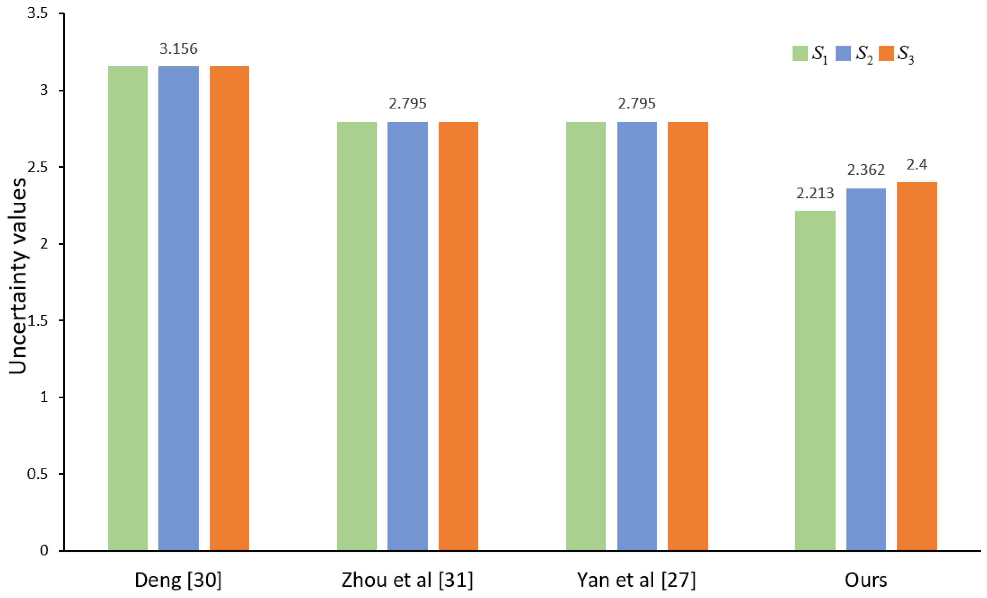
In the Example $1,$ for evidence $S_1,$ the intersection between three multi-element subsets is single element subset B. However, the intersection between two multi-elements subsets is single element subset B for evidence $S_2$ and $S_3$. For evidence $S_2,$ the intersection between multi-element subsets is single element subset B and $D,$ but it is single element subset A and B for evidence $S_3.$ What’s more, the probability of the basic probability assignment $m(B,D)$ is higher than $m(A,B)$ in BOEs. Based on the above analysis, it is obvious that the uncertainty of the three BOEs is not the same. However, the belief entropy of the three evidences is the same obtained by Deng entropy, Zhou et al.’s and Yan et al.’s belief entropy, which is contrary to common sense. Our proposed belief entropy can obtain a much more reasonable and satisfactory result, and the uncertainty of $S_1,S_2$ and $S_3$ increases in turn. This is in line with human intuition as shown in Figure 2.

Factors influencing the degree of uncertainty of evidence include the cardinality of the subset, the scale of BOE and the intersection between subsets. The three uncertainty measures fail to distinguish Example 1. The reason is that Deng entropy only considers the cardinality of the subset, while Zhou’s entropy just considers the cardinality of the subset and the scale of BOE. Although Yan’s entropy considers intrinsic connection between subsets in BOE, it only makes full use of the information of inclusion relationship between subsets and ignores the intersection between subsets. When there is only an intersection relationship among the subsets and no inclusion relationship, Yan’s entropy fails to distinguish Example 1 and can be degenerated into Zhou’s entropy. It is the reason that the uncertain value is the same obtained by Yan’s entropy and Zhou’s belief entropy. The comparison results of four uncertainty measures are given in

Table 2. Uncertainty measure of Example 1 with four entropies.

Uncertainty	${\mathit{S}}_1$	${\mathit{S}}_2$	${\mathit{S}}_3$
Deng entropy [30]	3.156	3.156	3.156
Zhou et al.’s belief entropy [31]	2.795	2.795	2.795
Yan et al.’s belief entropy [27]	2.795	2.795	2.795
Our proposed entropy	2.213	2.362	2.400

.

3.4.2. Counter-Example 2

Example 2.

Suppose the FOD is $\mathsf{\Theta }=\{A,B,C,D\}$,There is the inclusion and intersection relationship between propositions in BOEs.

$$\begin{array}{cc}\hfill & S_1:m_1(A,C)=0.3,m_1(B,C)=0.3,m_1(A,C,D)=0.4\hfill \\ \hfill & S_2:m_2(A,D)=0.3,m_2(B,C)=0.3,m_2(A,C,D)=0.4\hfill \\ \hfill & S_3:m_3(A,C)=0.3,m_3(B,C)=0.3,m_3(A,B,C,D)=0.4\hfill \\ \hfill & S_4:m_4(A,D)=0.3,m_4(B,C)=0.3,m_4(A,B,C,D)=0.4\hfill \end{array}$$

The belief entropy is calculated with Deng entropy as follows:

$E_d\left(m_1\right)=3.646$, $E_d\left(m_2\right)=3.646$, $E_d\left(m_3\right)=4.085$, $E_d\left(m_4\right)=4.085$

The belief entropy is calculated with Zhou et al.’s belief entropy as follows:

$$E_{Md}\left(m_1\right)=3.140,E_{Md}\left(m_2\right)=3.140,E_{Md}\left(m_3\right)=3.436,E_{Md}\left(m_4\right)=3.436$$

The belief entropy is calculated with Yan et al.’s belief entropy as follows:

$$H_n\left(m_1\right)=2.957,H_n\left(m_2\right)=2.957,H_n\left(m_3\right)=3.113,H_n\left(m_4\right)=3.113$$

The belief entropy is calculated with our proposed belief entropy as follows:

$H_p\left(m_1\right)=2.487$, $H_p\left(m_2\right)=2.636$, $H_p\left(m_3\right)=2.715$, $H_p\left(m_4\right)=2.864$

In the Example 2, evidence $S_1$ compared to evidence $S_2$, The number of multi-elements subsets whose intersection is single element subset C is greater. It is the same for evidence $S_3$ and evidence $S_4.$ Obviously, the uncertainty of evidence $S_1$ is different from that of evidence $S_2,$ and the uncertainty of evidence $S_3$ is different from that of evidence $S_4$.

The comparison results of different uncertainty measures are given in

Table 3. Uncertainty measure of Example 2 with four entropies.

Uncertainty	${\mathit{S}}_1$	${\mathit{S}}_2$	${\mathit{S}}_3$	${\mathit{S}}_4$
Deng entropy [30]	3.646	3.646	4.085	4.085
Zhou et al.’s belief entropy [31]	3.140	3.140	3.436	3.436
Yan et al.’s belief entropy [27]	2.957	2.957	3.113	3.113
Our proposed entropy	2.487	2.636	2.715	2.864

.

According to the results, we can conclude that the proposed belief entropy overcomes the limitations of the previous three methods, and could distinguish the uncertainty of four BOEs validly, on the contrary, the other three methods have failed. In addition, for the same BOE from Example 2, its degree of uncertainty calculated by four methods is monotonously decreasing. Because the latter method makes more use of the potential internal information in BOE.

3.4.3. Numerical Example 1

Example 3.

Suppose that the FOD is $\mathsf{\Theta }=\left\{A\right\}$ and the BPA is $m\left(A\right)=1.$ The values of Shannon entropy and the four entropies can be obtained as follows. The example is cited from [27].

$$\begin{array}{cc}\hfill & H\left(m\right)=-1\times {log}_{2}1=0\hfill \\ \hfill & E_d\left(m\right)=-1\times {log}_2\frac{1}{2-1}=0\hfill \\ \hfill & E_{Md}\left(m\right)=-1\times {log}_2\frac{1}{2-1}{e}^{\frac{1-1}{1}}=0\hfill \\ \hfill & H_p\left(m\right)=H_n\left(m\right)=-1\times {log}_2\frac{1+1}{2(2-1)}{e}^{\frac{1-1}{1}}=0\hfill \end{array}$$

As we can see from the results, when the FOD has only one single-element proposition, the value of uncertainty is 0. The four entropies and Shannon entropy get the same result.

3.4.4. Numerical Example 2

Example 4.

Suppose that the FOD is $\mathsf{\Theta }=\{A,B,C\}$ and the BPA is $m\left(A\right)=m\left(B\right)=m\left(C\right)=1/3.$ The values of Shannon entropy and the four entropies can be obtained as follows. The example is cited from [27].

$$\begin{array}{cc}\hfill & H\left(m\right)=-\frac{1}{3}{log}_2\frac{1}{3}-\frac{1}{3}{log}_2\frac{1}{3}-\frac{1}{3}{log}_2\frac{1}{3}=1.58\hfill \\ \hfill & H_p\left(m\right)=H_n\left(m\right)=E_{Md}\left(m\right)=E_d\left(m\right)=1.58\hfill \end{array}$$

The results of Example 3 and 4 show that the four entropies and Shannon entropy are the same when the BPA only consists of single-element propositions. At the same time, it also illustrates that PPT entropy retains the characteristics of Shannon entropy.

3.4.5. Numerical Example 3

Example 5.

Suppose that the FOD is $\mathsf{\Theta }=\left\{{\theta }_1,{\theta }_2\right\}.$ The BPA is $m\left({\theta }_1\right)=a,m\left({\theta }_2\right)=b,$$m\left(\mathsf{\Theta }\right)=1-a-b,$ where $a,b\in [0,0.5].$ Here, we calculate $E_d,E_{Md},H_n$ and $H_p$ values with the changes of a and b. The results are illustrated in Figure 1.

It is shown that the values of $E_{Md},H_n$ and $H_p$ are equal and smaller than that of $E_d$ when $a=b=0\left(m\right(\mathsf{\Theta })=1)$. This makes sense, because $E_{Md},H_n$ and $H_p$ all consider the influence of the scale of FOD on the uncertain measurement. In addition, the values of the four uncertainty measures change at different a and b, and are decreasing in turn. It is rational result, and the reason is analyzed as follows. Deng entropy only considers the influence of the cardinality of proposition on uncertainty measure. Zhou et al.’s belief entropy considers the influence of the cardinality of proposition and the scale of BOE. Yan et al.’s belief entropy considers the influence of the cardinality of proposition, the scale of BOE and the inclusion relationship among propositions. On the basis of Yan et al.’s belief entropy, our proposed belief entropy also considers the influence of the intersection relationship between propositions. Compared with the other three uncertainty measures, PPT entropy could dig up more information of the interaction of the internal elements in BOE, so the uncertainty value is the smallest.

3.4.6. Numerical Example 4

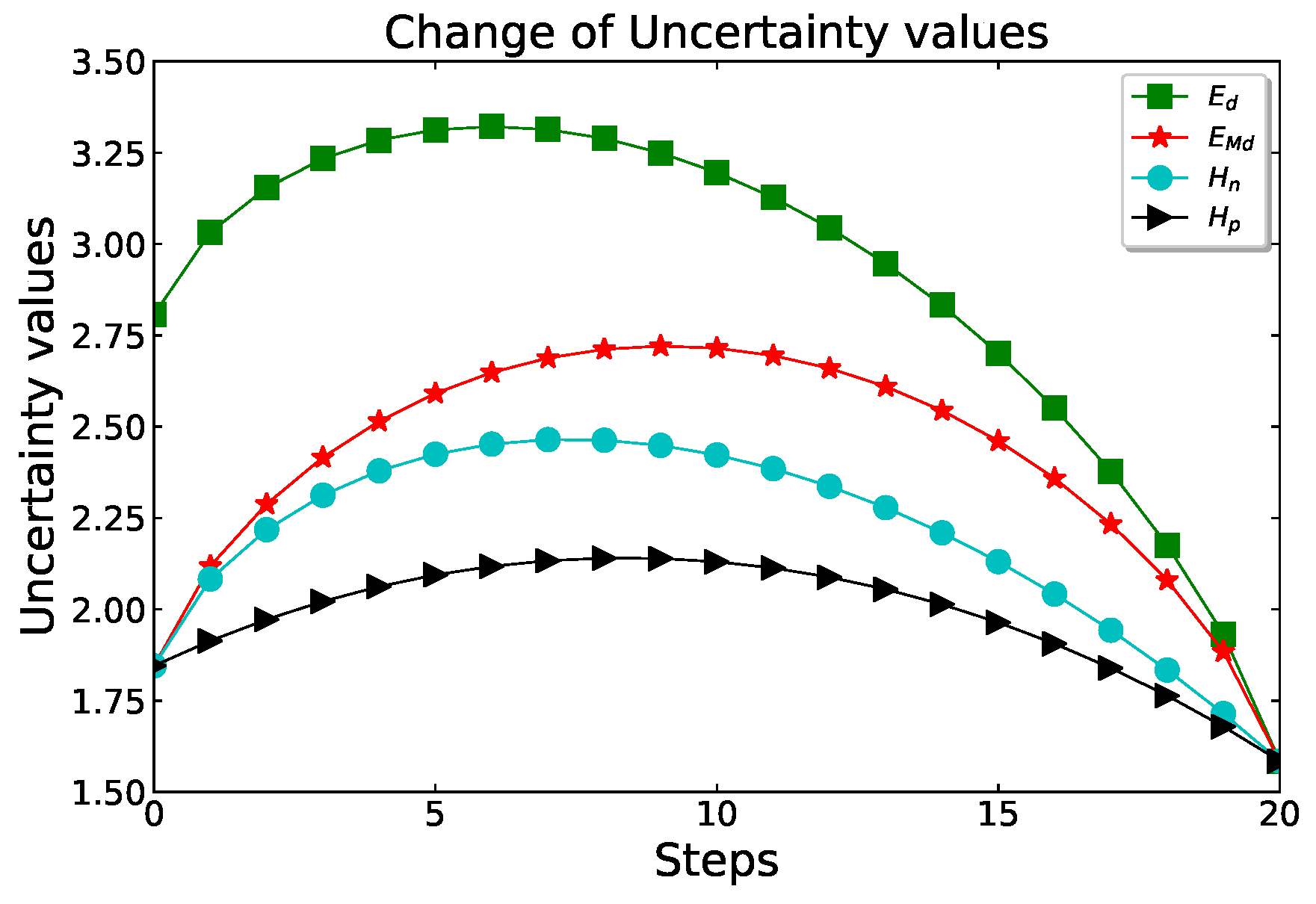
Example 6.

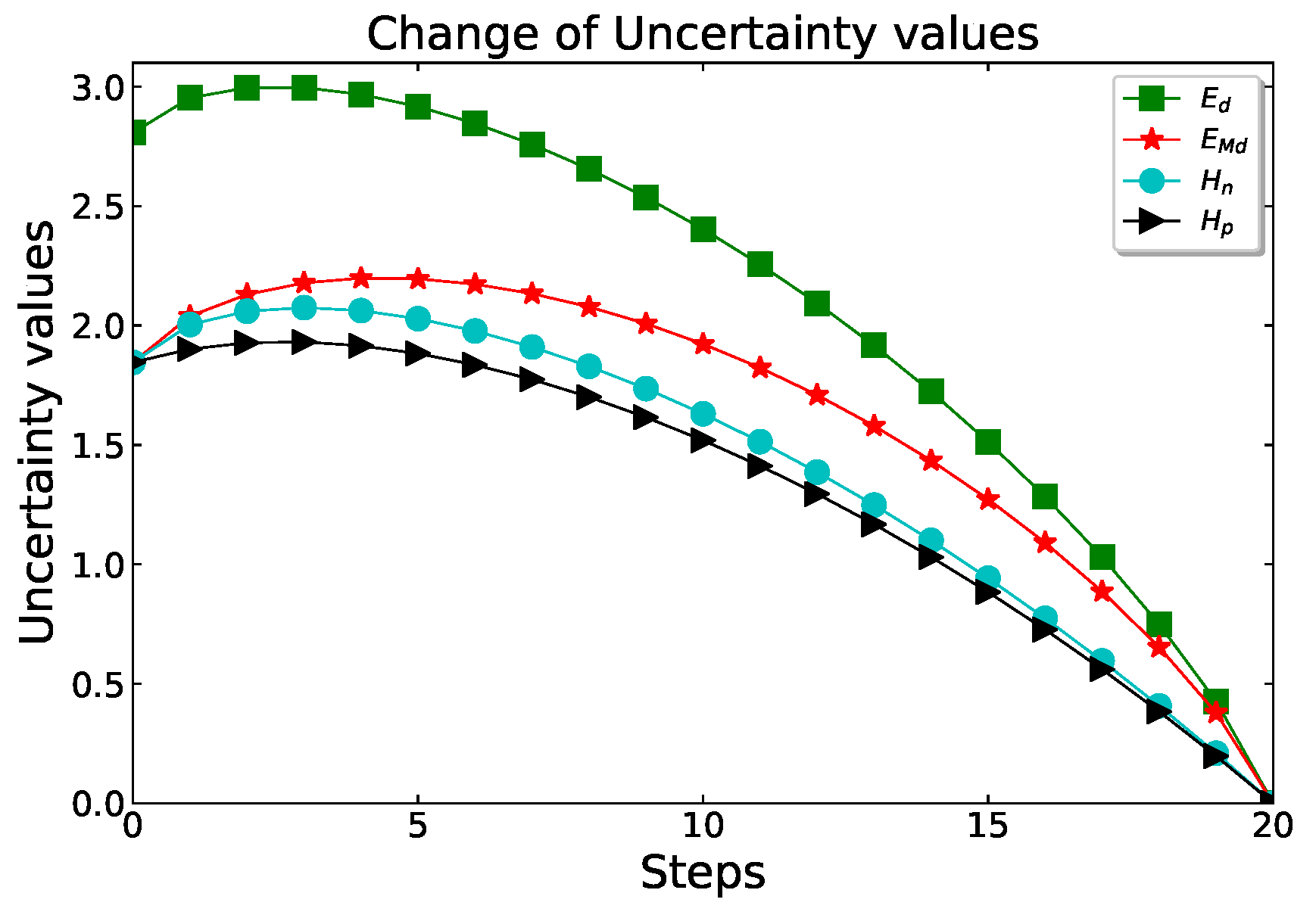
Suppose that the FOD is $\mathsf{\Theta }=\left\{{\theta }_1,{\theta }_2,{\theta }_3\right\}$ and the BPA is $m\left(\mathsf{\Theta }\right)=1$. We change the BPA step by step. In each step, $m\left(\mathsf{\Theta }\right)$ decreases $\Delta =0.05$ and each mass function $m\left({\theta }_i\right)$,i= 1, 2, 3 increases $\Delta /3.$ Finally, $m\left({\theta }_i\right)=1/3.$ The belief entropy is calculated with the four uncertainty measures. The changes of uncertainty values are shown in Figure 3.

For the four uncertainty measures, the uncertainty values of a vacuous BPA are all larger than that of a Bayesian one. This is intuitive, because the vacuous BPA represents that the information is completely unknown to the information system, while a Bayesian one could provide more certain information. It shows that PPT entropy inherits the advantages of Deng entropy, Zhou et.al’s belief entropy and Yan et.al’s belief entropy. Furthermore, when there is $m\left({\theta }_i\right)=1/3$, the uncertainty values of the four uncertainty measures is equal. It is also intuitive, because the four belief entropies are all degenerated into Shannon entropy when there are only single-element propositions in BOE as aforementioned in Example 4. With the change of the BPA in each step, $H_p$ is always at the minimum value among four uncertainty measures. Because it’s the only one that takes into account the effect of intersection between a multi-element proposition and single-element propositions on the uncertainty.

3.4.7. Numerical Example 5

Example 7.

The FOD is $\mathsf{\Theta }=\left\{{\theta }_1,{\theta }_2,{\theta }_3\right\}.$ The BPA is $m\left(\mathsf{\Theta }\right)=1$, and we change it step by step. In each step, $m\left(\mathsf{\Theta }\right)$ decreases $\Delta =0.05,$ and $m\left({\theta }_1\right)$ increases $\Delta =0.05$. Repeat the process until $m\left({\theta }_1\right)=1$. The belief entropy is calculated with the four uncertainty measures. The changes of uncertainty values are shown in Figure 4.

The values of $E_d,E_{Md}$, $H_n$ and $H_p$ all change with the change of the BPA in each step. The uncertainty values of a vacuous BPA are larger than that of a categorical one. It is intuitive, because a vacuous BPA means completely unknown, and a categorical one means to be pretty certain. When there is $m\left({\theta }_1\right)=1$, the uncertainty values of different uncertainty measures all change to zero. It is also intuitive, because the four belief entropies are all degenerated into Shannon entropy when there is only one single-element proposition as aforementioned in Example 3. It once again illustrates that the PPT entropy retains the characteristics of Shannon entropy.

3.4.8. Numerical Example 6

Example 8.

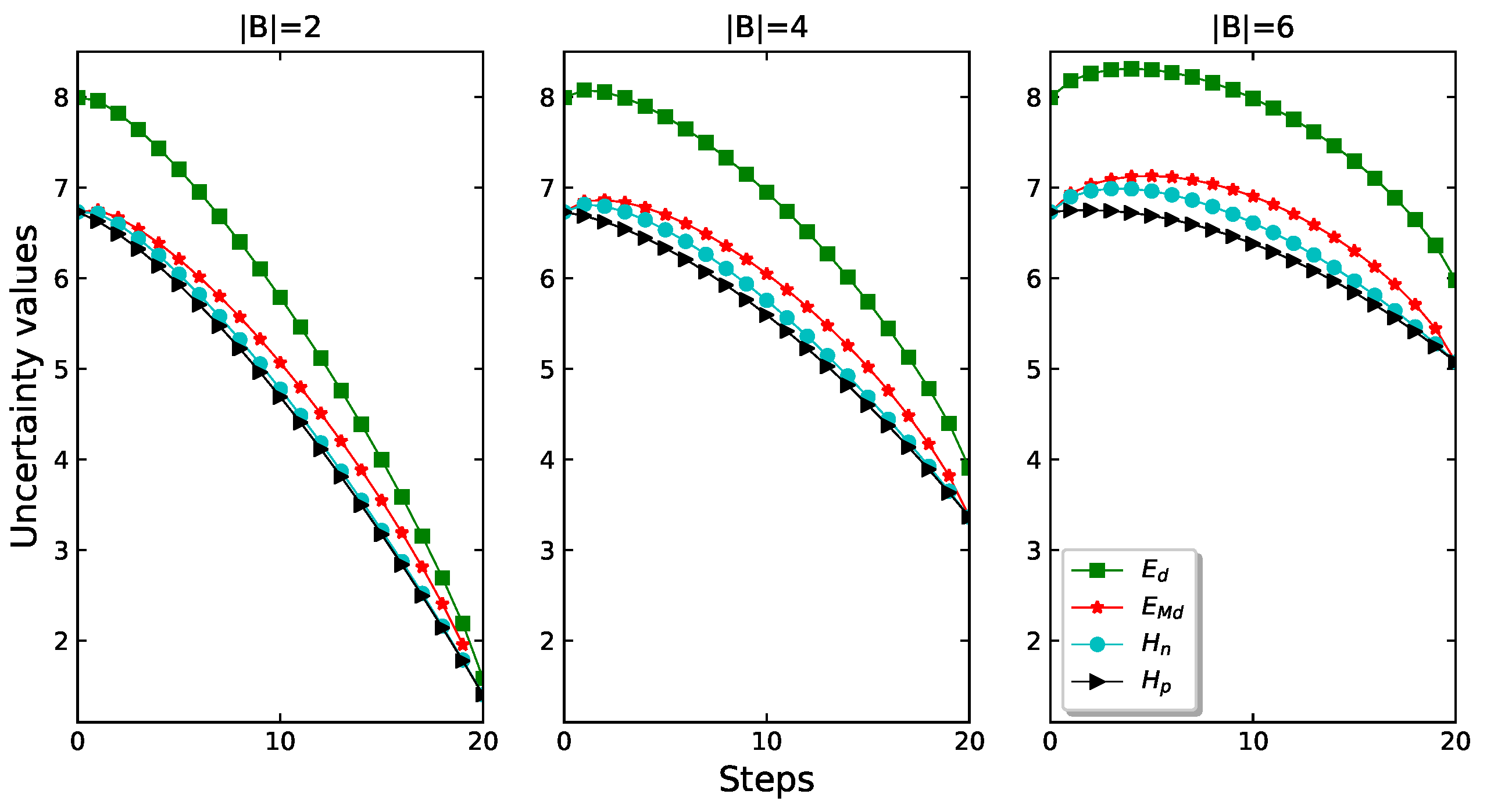
Suppose that the FOD is $\mathsf{\Theta }=\left\{{\theta }_1,\dots ,{\theta }_8\right\}.$ The BPA is $m\left(\mathsf{\Theta }\right)=1,$ and we change it step by step. In each step, $m\left(\mathsf{\Theta }\right)$ decreases $\Delta =0.05,$ and $m\left(B\right)$ increases $\Delta =0.05$. The cardinality of proposition B is 2, 4 and 6, respectively. Repeat the process until $m\left(B\right)=1$. The changes of values for the four uncertainty measures under the different $\left|B\right|$ are shown in Figure 5.

As shown in Figure 5, when $\left|B\right|$ has a smaller value, the values of $E_d,E_{Md},H_n$ and $H_p$ will change faster at each step. Because the same mass assignments are assigned to a smaller cardinality proposition. When there is one multi-element proposition in BOE, i.e., $m\left(\mathsf{\Theta }\right)=1$ or $m\left(B\right)=1$, the values of $E_{Md},H_n$ and $H_p$ is equal. However, $E_d$ is different from the other uncertainty measures. Because it is no interaction between propositions when there is only one multi-element proposition, and the scale of FOD plays a decisive role in uncertainty measure. Only $E_d$ does not consider the influence of the scale of FOD on the uncertain measurement. what’s more, the uncertainty value of $H_p$ is always the smallest, which illustrates that the PPT entropy has a less information loss than other uncertainty measures and the result is most accurate.

3.4.9. Numerical Example 7

Example 9.

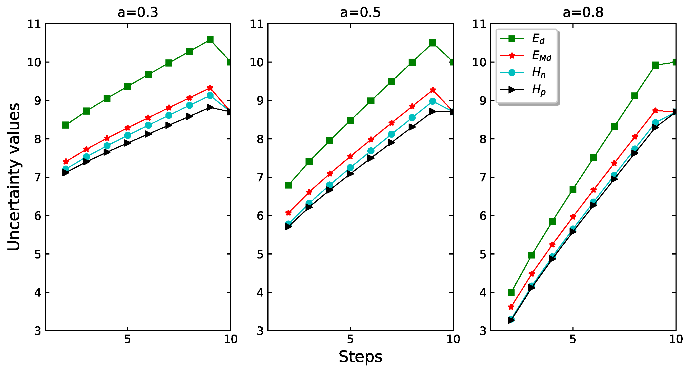
Suppose that the FOD is $\mathsf{\Theta }=\left\{{\theta }_1,\dots ,{\theta }_{10}\right\}$. The BPA is $m\left(\mathsf{\Theta }\right)=1-a$ and $m\left(A\right)=a$. Given an a value, and we change the BPA step by step. $\left|A\right|$ changes from 1 to 10, and increases by 1 in each step. We set $a=0.3,0.5,0.8,$ respectively. Under the different a, the changes of values for the four uncertainty measures are shown in Figure 6.

As shown in Figure 6, the values of $E_d,E_{Md},H_n$ and $H_p$ all increase with the increase of $\left|A\right|$ at the first 8 steps and decrease or increase in the last. The reasons are described as follows. According to the monotonicity, the uncertainty of BOE which consists of two multi-element propositions is undoubtedly increasing at the first 8 steps. Comparatively, due to the BPA is shifted from two multi-element propositions to one multi-element proposition in the last step, the changes in uncertainty are inconsistent and may be large or small. If a has a larger value, they will increase even more, because relatively more mass assignments are assigned to a larger cardinality proposition. In addition, we can see that the values of $H_n$ and $H_p$ are getting closer and closer, and they almost overlap at some points, as a increases. Because the intersection between multi-element propositions has less influence on the uncertainty when the $m\left(\mathsf{\Theta }\right)$ is decreasing.

3.4.10. Numerical Example 8

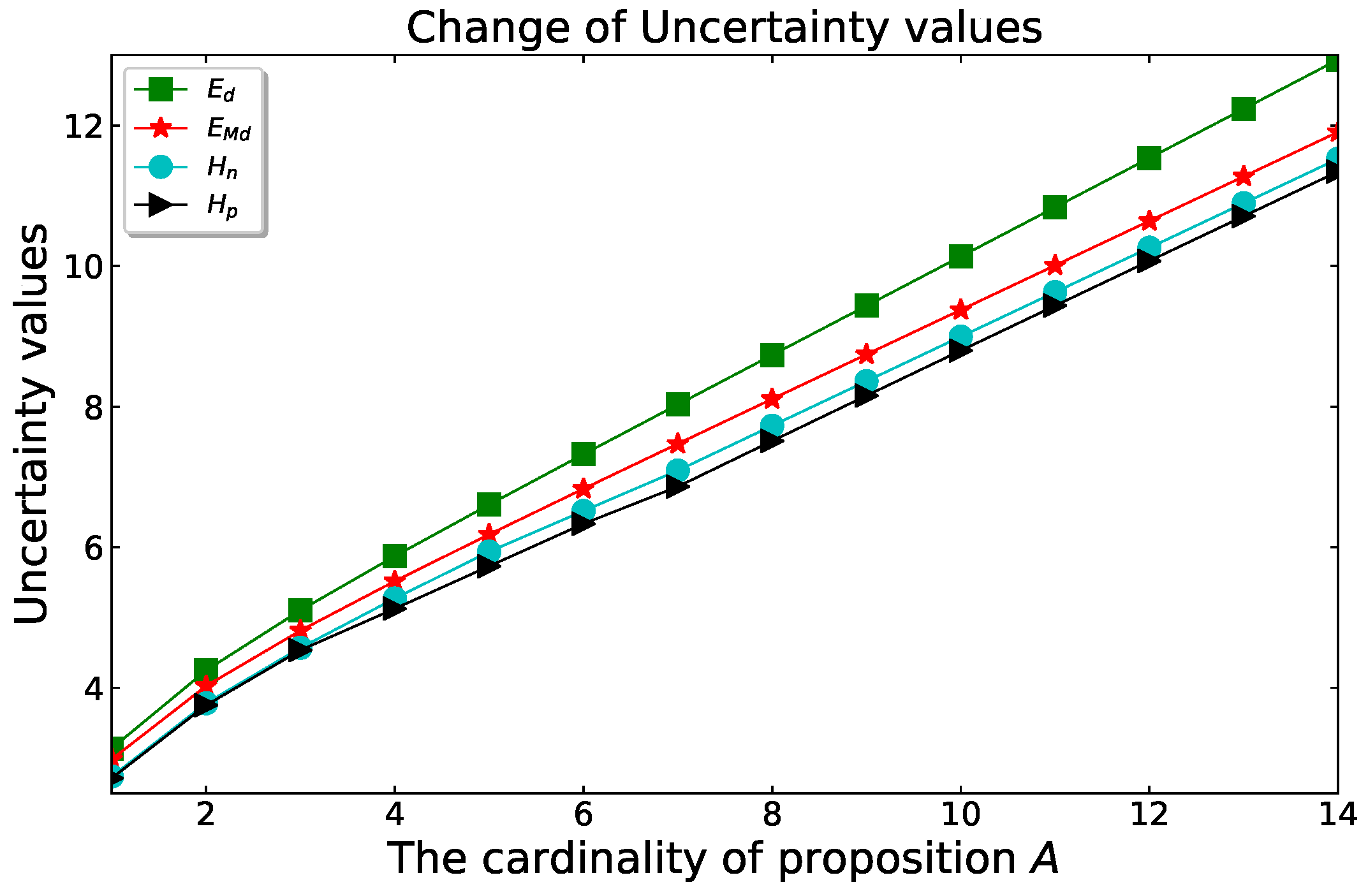
Example 10.

Suppose that the FOD is $\mathsf{\Theta }=\{1,2,\dots ,14,15\}$, and the BPA is shown as follows:

$m(4,5,6)=0.1,m\left(7\right)=0.1,m($A$)=0.7,m(\mathsf{\Theta })=0.1$where A represents a proposition, and the cardinality of proposition A is variable from 1 to 14. The example is cited from [27]. The belief entropy is calculated with the four uncertainty measures that is shown in Figure 7.

As we can see in Figure 7, with the cardinality of proposition A continuing to increase, the values of $E_d$, $E_{Md}$, $H_n$ and $H_p$ increase monotonically which further illustrates the monotonicity of PPT entropy. Furthermore, by taking into consideration of the intersection between propositions, the PPT entropy takes advantage of more valuable information in BOE and the uncertain degree is always smaller than the other three uncertainty measures, which ensures it to be more reasonable and effective for uncertainty measure.

3.5. Entropy Distance

In this paper, we introduce the concept of entropy distance. It is a novel distance measurement method and is used to measure the difference between belief entropy of evidences, thereby characterizing the degree of conflict between evidences from the perspective of mutual belief entropy. The more similar between BOEs, the smaller the entropy distance between BOEs.

Suppose that $A_1,A_2,\cdots ,A_K$ are the focal element of the BPAs $m_i$ and $m_j$, then the entropy distance between $m_i$ and $m_j$ is defined as follows:

$$d_H\left(m_i,m_j\right)=\underset{A_K\subseteq \mathsf{\Theta }}{max}\left\{\left|H_p\left(m_i\left(A_k\right)\right)-H_p\left(m_j\left(A_k\right)\right)\right|\right\}$$

(13)

$H_{\mathrm{p}}\left(m_i\left(A_k\right)\right)$ is belief entropy of the focal element $A_k$, and $d_H\left(m_i,m_j\right)$ denotes the maximum value of the difference in belief entropy of the corresponding focal element. Entropy distance, as a novel distance measurement method, has the following two advantages than relative entropy [42]. On the one hand, the entropy distance satisfies the symmetry. On the other hand, it can measure the difference of two BOEs more accurately and in a wider range. Next, an example is used to verify the advantages of entropy distance.

Example 11.

Suppose that the FOD is $\mathsf{\Theta }=\{A,B,C\}$.

$$\begin{array}{cc}\hfill & S_1:m_1(A,B)=0.3,m_1(A,C)=0.7\hfill \\ \hfill & S_2:m_2(A,B)=0.8,m_2(A,C)=0.2\hfill \\ \hfill & S_3:m_3(A,B)=0.3,m_3\left(C\right)=0.7\hfill \\ \hfill & S_4:m_4(A,B)=0.8,m_4\left(C\right)=0.2\hfill \\ \hfill & S_5:m_5\left(A\right)=0.1,m_5\left(B\right)=0,m_5\left(C\right)=0.9\hfill \\ \hfill & S_6:m_6\left(A\right)=0.1,m_6\left(B\right)=0.9,m_6\left(C\right)=0\hfill \end{array}$$

The distance value between $m_1$ and $m_2$ is calculated with relative entropy as follows:

$$\begin{array}{cc}\hfill & \mathrm{KL}(m_1\parallel m_2)=\sum m_1\left(A\right){log}_2\frac{m_1\left(A\right)}{m_2\left(A\right)}=0.3{log}_2\frac{0.3}{0.8}+0.7{log}_2\frac{0.7}{0.2}=0.841\hfill \\ \hfill & \mathrm{KL}(m_2\parallel m_1)=\sum m_2\left(A\right){log}_2\frac{m_2\left(A\right)}{m_1\left(A\right)}=0.8{log}_2\frac{0.8}{0.3}+0.2{log}_2\frac{0.2}{0.7}=0.771\hfill \end{array}$$

The distance value between $m_3$ and $m_4$ is calculated with relative entropy as follows:

$$\mathrm{KL}(m_3\parallel m_4)=0.3{log}_2\frac{0.3}{0.8}+0.7{log}_2\frac{0.7}{0.2}=0.841$$

The distance value between $m_5$ and $m_6$ is calculated with relative entropy as follows:

$$\mathrm{KL}(m_5\parallel m_6)=0.1{log}_2\frac{0.1}{0.1}+0\times {log}_2\frac{0}{0.9}+0.9{log}_2\frac{0.9}{0}=NaN$$

The distance value between $m_1$ and $m_2$ is calculated with entropy distance as follows:

$$\begin{array}{cc}\hfill d_H\left(m_1,m_2\right)=& \underset{A_K\subseteq \mathsf{\Theta }}{max}\left\{\left|H_p\left(m_1\left(A_k\right)\right)-H_p\left(m_2\left(A_k\right)\right)\right|\right\}\hfill \\ \hfill =& max\{\left|-0.3{log}_2\frac{0.3+0.3+\frac{1}{2}\times 0.7}{2(2^2-1)}{e}^{\frac{2-1}{3}}+0.8{log}_2\frac{0.8+0.8+\frac{1}{2}\times 0.2}{2(2^2-1)}{e}^{\frac{2-1}{3}}\right|,\hfill \\ \hfill & \left|-0.7{log}_2\frac{0.7+0.7+\frac{1}{2}\times 0.3}{2\left(2^2-1\right)}{e}^{\frac{2-1}{3}}+0.2{log}_2\frac{0.2+0.2+\frac{1}{2}\times 0.8}{2\left(2^2-1\right)}{e}^{\frac{2-1}{3}}\right|\}\hfill \\ \hfill =& max\left\{\right|-0.417|,|0.545\left|\right\}\hfill \\ \hfill =& 0.545\hfill \\ \hfill =& d_H\left(m_2,m_1\right)\hfill \end{array}$$

The distance value between $m_3$ and $m_4$ is calculated with entropy distance as follows:

$$d_H\left(m_3,m_4\right)=max\left\{\right|-1.088|,|-0.104\left|\right\}=1.088$$

The distance value between $m_5$ and $m_6$ is calculated with entropy distance as follows:

$$d_H\left(m_5,m_6\right)=max\left\{\right|0|,|-0.137|,|0.137\left|\right\}=0.137$$

The distance value between $m_1$ and $m_2$ obtained by the entropy distance is the same as $m_2$ and $m_1$, which proves that entropy distance satisfies the symmetry, however, relative entropy does not. The difference between $m_1$ and $m_2$ is intuitively different from the difference between $m_3$ and $m_4$, but the two distance values obtained by the relative entropy are both equal to 0.841. The two distance values obtained by the entropy distance is not equal, which illustrates that our proposed method can distinguish two situations and measure the difference of two BOEs more accurately. Since the denominator is 0, the distance value between $m_5$ and $m_6$ can not be calculated with relative entropy. In contrast, the distance value between the two BOEs can be measured by entropy distance, which verifies that the entropy distance measures the difference of two BOEs in a wider range. The comparison results of two distance methods are given in

Table 4. The comparison results of two distance methods.

Method	${\mathit{S}}_1,{\mathit{S}}_2$	${\mathit{S}}_2,{\mathit{S}}_1$	${\mathit{S}}_3,{\mathit{S}}_4$	${\mathit{S}}_5,{\mathit{S}}_6$
relative entropy [42]	0.841	0.771	0.841	NaN
entropy distance	0.545	0.545	1.088	0.137

.

Comparing to the existing methods based on belief entropy itself, entropy distance measures the conflict between evidences from a global point of view, entropy distance measures the conflict between evidences from a local perspective. With introducing entropy distance into conflict management, conflicts are measured from a global and local point of view, and conflict measurement could be more accurate and comprehensive. Even though the belief entropy of conflict evidence and normal evidence is equal or close, it can still effectively identify conflict evidence.

3.6. Proposed Method for Conflict Management Based on PPT Entropy and Entropy Distance

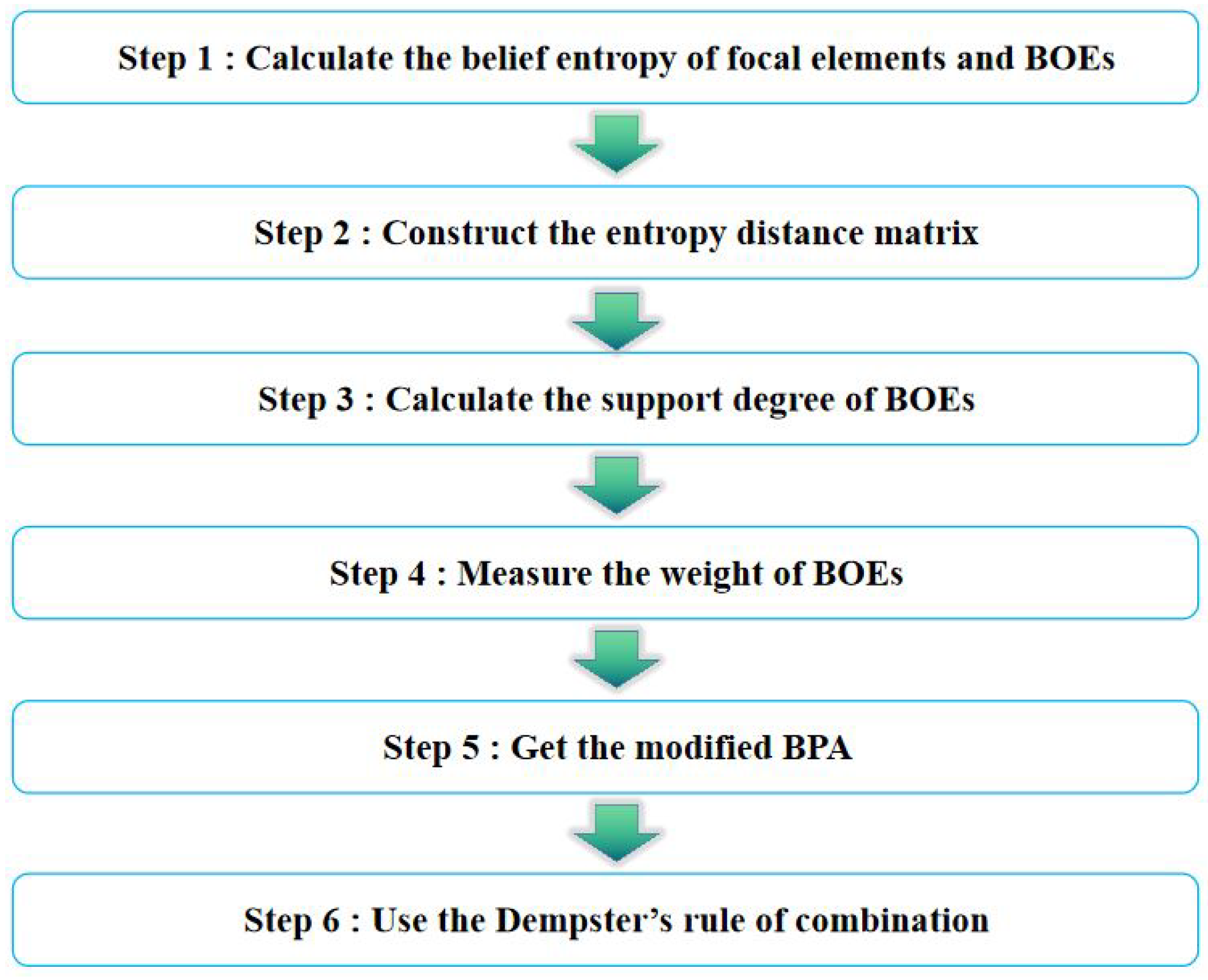
The flowchart of the proposed conflict management approach based on PPT entropy and entropy distance is given in Figure 8.

Suppose that $\mathsf{\Theta }$ is the FOD and there are n pieces of evidences.

• Calculate the belief entropy of focal elements and BOEs with Equation (12).
• Construct entropy distance matrix with Equation (14).

  $$D_{n\times n}=\left[\begin{array}{cccc}0& d_H\left(m_1,m_2\right)& \cdots & d_H\left(m_1,m_n\right)\\ d_H\left(m_2,m_1\right)& 0& \cdots & d_H\left(m_2,m_n\right)\\ ⋮& ⋮& ⋮& ⋮\\ d_H\left(m_n,m_1\right)& d_H\left(m_n,m_2\right)& \cdots & 0\end{array}\right]$$

  (14)
• Calculate the support degree of BOEs with Equation (15).

  $$Sup\left(m_i\right)=\frac{H_p\left(m_i\right)}{{\sum }_{j=1}^n{d}_H\left(m_i,m_j\right)}$$

  (15)
  $Sup\left(m_i\right)$ represents the support degree of BOE $m_i$. It is a fractional form in which PPT entropy is treated as a numerator and sum of entropy distance as a denominator. Entropy distance is inversely proportional to the weight of evidence. This is consistent with the intuitive analysis results. Whereas, For the existing methods, the support degree of BOE is calculated by Equation (16) and is equal to belief entropy itself.

  $$Sup\left(m_i\right)=H^{\prime }\left(m_i\right)$$

  (16)
  $H^{\prime }\left(m_i\right)$ represents different belief entropies.
• Measure the weight value of BOEs with Equation (17).

  $$w_i=\frac{Sup\left(m_i\right)}{{\sum }_{i=1}^{n}Sup\left(m_i\right)}$$

  (17)
• Get the modified BPA with Equation (18).

  $$m\left(A\right)=\sum _{i=1}^n{w}_i\times m_i\left(A\right)$$

  (18)
• Use the Dempster’s rule of combination with Equation (4), we combine the modified BPA n − 1 times.

3.7. Experiments

3.7.1. Numerical Example 9

Example 12.

Suppose that in the same frame of discernment $\mathsf{\Theta }=\{A,B,C\},$ the system has obtained the data information from four different types of sensors, and the BPA of each sensor data is shown in

Table 5. The BPA of multi-sensor data.

	A	B	C
$m_1$	0.9	0.1	0
$m_2$	0	0.9	0.1
$m_3$	0.9	0.1	0
$m_4$	0.9	0.1	0

. Intuitively, the evidence $m_2$ is highly conflicting with other evidence and the hypothesis A will be obtained the highest belief.

According to the proposed method, the specific calculation process is shown below.

Step 1: Calculate the belief entropy of focal elements and BOEs.

The belief entropy of focal elements can be obtained as follows:

$$\begin{gathered} H_p\left(m_1\left(A\right)\right)=0.131,H_p\left(m_1\left(B\right)\right)=0.332 \\ {H}_p\left(m_2\left(B\right)\right)=0.131,H_p\left(m_2\left(C\right)\right)=0.332 \\ {H}_p\left(m_3\left(A\right)\right)=0.131,H_p\left(m_3\left(B\right)\right)=0.332 \\ {H}_p\left(m_4\left(A\right)\right)=0.131,H_p\left(m_4\left(B\right)\right)=0.332 \end{gathered}$$

The belief entropy of BOEs can be obtained as follows:

$H_p\left(m_1\right)=0.469$, $H_p\left(m_2\right)=0.469$, $H_p\left(m_3\right)=0.469$, $H_p\left(m_4\right)=0.469$

Step 2: Construct the entropy distance matrix $D_{4\times 4}$.

$${\mathrm{D}}_{4\times 4}=\left[\begin{array}{cccc}0& 0.332& 0& 0\\ 0.332& 0& 0.332& 0.332\\ 0& 0.332& 0& 0\\ 0& 0.332& 0& 0\end{array}\right]$$

Step 3: Calculate the support degree of BOEs.

$Sup\left(m_1\right)=1.413$, $Sup\left(m_2\right)=0.471$, $Sup\left(m_3\right)=1.413$, $Sup\left(m_4\right)=1.413$

Step 4: Measure the weight of the four BOEs.

$w_1=0.3$, $w_2=0.1$, $w_3=0.3$, $w_4=0.3$

Step 5: Get the modified BPA.

$m\left(A\right)=0.81,m\left(B\right)=0.18,m\left(C\right)=0.01$

Step 6: Use the Dempster’s rule of combination to combine the modified BPA 3 times.

$$\begin{gathered} m\left(A\right)={\left({\left({(m\oplus m)}_1\oplus m\right)}_2\oplus m\right)}_3\left(A\right)=1 \\ m\left(B\right)={\left({\left({(m\oplus m)}_1\oplus m\right)}_2\oplus m\right)}_3\left(B\right)=0 \\ m\left(C\right)={\left({\left({(m\oplus m)}_1\oplus m\right)}_2\oplus m\right)}_3\left(C\right)=0 \end{gathered}$$

The fusion results of four BPAs with different methods are shown in the

Table 6. The result of combining conflicting evidence with different methods in the Example 12.

Method	${\mathit{m}}_1,{\mathit{m}}_2$	${\mathit{m}}_1,{\mathit{m}}_2,{\mathit{m}}_3$	${\mathit{m}}_1,{\mathit{m}}_2,{\mathit{m}}_3,{\mathit{m}}_4$
Existing methods [27,28,29]	$w_1=w_2=0.5$	$w_1=w_3=0.33,w_2=0.34$	$w_1=w_2=w_3=w_4=0.25$
	$m\left(a\right)=0.445$	$m\left(a\right)=0.814$	$m\left(a\right)=0.962$
	$m\left(b\right)=0.550$	$m\left(b\right)=0.186$	$m\left(b\right)=0.038$
	$m\left(c\right)=0.005$	$m\left(c\right)=0.000$	$m\left(c\right)=0.000$
Proposed method	$w_1=w_2=0.5$	$w_1=w_3=0.4,w_2=0.2$	$w_1=w_3=w_4=0.3,w_2=0.1$
	$m\left(a\right)=0.445$	$m\left(a\right)=0.955$	$m\left(a\right)=1.000$
	$m\left(b\right)=0.550$	$m\left(b\right)=0.045$	$m\left(b\right)=0.000$
	$m\left(c\right)=0.005$	$m\left(c\right)=0.000$	$m\left(c\right)=0.000$

.

In this example, the belief entropy of four evidences is 0.469 according to the calculated results. Obviously, the belief entropy of conflict evidence and normal evidence is equal. As seen from the results, the existing methods can obtain correct result. However, the same weight is allocated to each evidence which makes conflicting evidence fail to be effectively handled in the subsequent fusion process. The reason is that the existing methods are only using belief entropy itself as the support degree to assign the weight of evidence.

Compared with existing methods, a smaller weight of conflicting evidence $m_2$ is obtained by our proposed approach, which reduces the impact of conflict evidence on subsequent evidence combination. It not only has better convergence performance, but also obtain the higher belief degree of the hypothesis A by $100\%$. The feasibility of the proposed method of conflict management is verified.

3.7.2. Numerical Example 10

Example 13.

Suppose that in the same frame of discernment $\mathsf{\Theta }=\{A,B,C\},$ the system has obtained the data information from five different types of sensors [43], and the BPA of each sensor data is shown in

Table 7. The basic probability assignment (BPA) of multi-sensor data.

	A	B	C	{A,C}	{B,C}
$m_1$	0.65	0.05	0.25	0.05	0
$m_2$	0.55	0.10	0	0.35	0
$m_3$	0	0.60	0.10	0	0.30
$m_4$	0.55	0.10	0	0.35	0
$m_5$	0.55	0.10	0	0.35	0

. Intuitively, the evidence $m_3$ is highly conflicting with other evidence and the hypothesis A will be obtained the highest belief. The example is cited from [43].

The fusion results of five BPAs with different methods are shown in the

Table 8. The result of combining conflicting evidence with different methods in the Example 13.

Method	${\mathit{m}}_1,{\mathit{m}}_2$	${\mathit{m}}_1,{\mathit{m}}_2,{\mathit{m}}_3$	${\mathit{m}}_1,{\mathit{m}}_2,{\mathit{m}}_3,{\mathit{m}}_4$	${\mathit{m}}_1,{\mathit{m}}_2,{\mathit{m}}_3,{\mathit{m}}_4,{\mathit{m}}_5$
Existing methods [27,28,29]	$m\left(a\right)=0.843$	$m\left(a\right)=0.576$	$m\left(a\right)=0.899$	$m\left(a\right)=0.966$
	$m\left(b\right)=0.008$	$m\left(b\right)=0.228$	$m\left(b\right)=0.026$	$m\left(b\right)=0.004$
	$m\left(c\right)=0.095$	$m\left(c\right)=0.181$	$m\left(c\right)=0.067$	$m\left(c\right)=0.026$
	$m(a,c)=0.054$	$m(a,c)=0.009$	$m(a,c)=0.008$	$m(a,c)=0.004$
	$m(b,c)=0.000$	$m(b,c)=0.006$	$m(b,c)=0.000$	$m(b,c)=0.000$
Proposed method	$m\left(a\right)=0.843$	$m\left(a\right)=0.704$	$m\left(a\right)=0.934$	$m\left(a\right)=0.982$
	$m\left(b\right)=0.008$	$m\left(b\right)=0.129$	$m\left(b\right)=0.010$	$m\left(b\right)=0.001$
	$m\left(c\right)=0.095$	$m\left(c\right)=0.153$	$m\left(c\right)=0.046$	$m\left(c\right)=0.012$
	$m(a,c)=0.054$	$m(a,c)=0.011$	$m(a,c)=0.010$	$m(a,c)=0.005$
	$m(b,c)=0.000$	$m(b,c)=0.003$	$m(b,c)=0.000$	$m(b,c)=0.000$

.

As seen from the results, the convergence speed of the proposed method is faster and $m\left(a\right)=0.704$ after three evidences including the conflict evidence $m_3$ are combined, which is higher than that of the existing approaches. What’s more, the combination results can promptly converge to the desired value with the increasing number of evidences, $m\left(a\right)=0.934$ after four evidences are combined, and $m\left(a\right)=0.982$ after five evidences are fused. The belief degree of the hypothesis A increases by $1.6\%$ compared to existing methods. The reason is that our proposed method comprehensively considers the impact of the self-belief entropy and mutual belief entropy on conflict management. It not only can measure the degree of conflict between evidences effectively, but also can strengthen the influence of normal evidence further and at the same time weaken the influence of conflicting evidence further. Additionally, the belief entropy of five evidences is 1.190, 1.238, 1.109, 1.238 and 1.238 by the calculation, respectively. Obviously, the belief entropy of a conflict evidence and normal evidences is close. So we can conclude from Table 6 and 8 that conflict can be effectively handled, whether the belief entropy of conflict evidence and normal evidence is equal or close. The robustness and superiority of the proposed approach is fully illustrated.

4. Application

In this section, the effectiveness of the proposed method in the application of target recognition is shown. Not only the results are consistent with existing method, but also the belief degree of the true target is improved. The example is cited [15,24,26,28,29].

Example 14.

In a multi-target recognition system, three targets are denoted as$A,B$andC. Suppose that there is a total of five sensors, respectively obtaining five pieces of evidences. The BPA of each sensor data is shown in

Table 9. The BPA of multi-sensor data.

	A	B	C	{A, C}
$m_1$	0.41	0.29	0.30	0
$m_2$	0	0.90	0.10	0
$m_3$	0.58	0.07	0	0.35
$m_4$	0.55	0.10	0	0.35
$m_5$	0.60	0.10	0	0.30

. Intuitively, the evidence$m_2$is highly conflicting with other evidence and the targetAwill be obtained the highest belief.

According to the proposed method, the specific calculation process is shown below.

Step 1: Calculate the belief entropy of focal elements and BOEs.

$$\begin{array}{cc}\hfill H_p\left(m_1\left(A\right)\right)& =0.527,H_p\left(m_1\left(B\right)\right)=0.518,H_p\left(m_1\left(C\right)\right)=0.521,H_p\left(m_1\right)=1.566\hfill \\ \hfill H_p\left(m_2\left(A\right)\right)& =0.000,H_p\left(m_2\left(B\right)\right)=0.137,H_p\left(m_2\left(C\right)\right)=0.332,H_p\left(m_2\right)=0.469\hfill \\ \hfill H_p\left(m_3\left(A\right)\right)& =0.338,H_p\left(m_3\left(B\right)\right)=0.269,H_p\left(m_3(A,C)\right)=0.612,H_p\left(m_3\right)=1.219\hfill \\ \hfill H_p\left(m_4\left(A\right)\right)& =0.357,H_p\left(m_4\left(B\right)\right)=0.332,H_p\left(m_4(A,C)\right)=0.624,H_p\left(m_4\right)=1.313\hfill \\ \hfill H_p\left(m_5\left(A\right)\right)& =0.340,H_p\left(m_5\left(B\right)\right)=0.332,H_p\left(m_5(A,C)\right)=0.552,H_p\left(m_5\right)=1.224\hfill \end{array}$$

Step 2: Establish the entropy distance matrix $D_{5\times 5}$.

$${\mathrm{D}}_{5\times 5}=\left[\begin{array}{ccccc}0& 0.527& 0.612& 0.624& 0.552\\ 0.527& 0& 0.612& 0.624& 0.552\\ 0.612& 0.612& 0& 0.063& 0.063\\ 0.624& 0.624& 0.063& 0& 0.072\\ 0.552& 0.552& 0.063& 0.072& 0\end{array}\right]$$

Step 3: Calculate the support degree of BOEs.

$Sup\left(m_1\right)=0.677$, $Sup\left(m_2\right)=0.202$, $Sup\left(m_3\right)=0.903$, $Sup\left(m_4\right)=0.949$, $Sup\left(m_5\right)=0.988$

Step 4: Measure the weight of the five BOEs.

$$w_1=0.182,w_2=0.054,w_3=0.243,w_4=0.255,w_5=0.266$$

Step 5: Get the modified BPA.

$$m\left(A\right)=0.515,m\left(B\right)=0.171,m\left(C\right)=0.060,m(A,C)=0.254$$

Step 6: Use the Dempster’s rule of combination to combine the modified BPA 4 times.

$$m\left(A\right)=0.988,m\left(B\right)=0.001,m\left(C\right)=0.007,m(A,C)=0.004$$

The fusion results of five BPAs with different methods are shown in

Table 10. The result of combining conflicting evidence with different methods in the Example 14.

Method	${\mathit{m}}_1,{\mathit{m}}_2$	${\mathit{m}}_1,{\mathit{m}}_2,{\mathit{m}}_3$	${\mathit{m}}_1,{\mathit{m}}_2,{\mathit{m}}_3,{\mathit{m}}_4$	${\mathit{m}}_1,{\mathit{m}}_2,{\mathit{m}}_3,{\mathit{m}}_4,{\mathit{m}}_5$
Existing methods [27,28,29]	$m\left(a\right)=0.286$	$m\left(a\right)=0.762$	$m\left(a\right)=0.935$	$m\left(a\right)=0.982$
	$m\left(b\right)=0.529$	$m\left(b\right)=0.122$	$m\left(b\right)=0.017$	$m\left(b\right)=0.002$
	$m\left(c\right)=0.185$	$m\left(c\right)=0.105$	$m\left(c\right)=0.040$	$m\left(c\right)=0.013$
	$m(a,c)=0.000$	$m(a,c)=0.011$	$m(a,c)=0.008$	$m(a,c)=0.003$
Proposed method	$m\left(a\right)=0.286$	$m\left(a\right)=0.746$	$m\left(a\right)=0.950$	$m\left(a\right)=0.988$
	$m\left(b\right)=0.529$	$m\left(b\right)=0.136$	$m\left(b\right)=0.009$	$m\left(b\right)=0.001$
	$m\left(c\right)=0.185$	$m\left(c\right)=0.108$	$m\left(c\right)=0.031$	$m\left(c\right)=0.007$
	$m(a,c)=0.000$	$m(a,c)=0.010$	$m(a,c)=0.010$	$m(a,c)=0.004$

.

As can be seen from Table 10, the recognized target by our improved approach is consistent with existing method. On this basis, the belief degree of the true target is also improved from $98.2\%$ to $98.8\%$, the greater the conflict between evidences, the greater the performance improvement as shown in Example 12 and 13. Two reasons for the effectiveness of the proposed method are given. On the one hand, we measure conflict between evidences from the overall and local point of view so that the conflicts can be accurately measured. On the other hand, the introduction of entropy distance makes the difference between evidences more precise,and conflicting evidences can be assigned a smaller weight than normal evidences. Furthermore, according to the calculation results, the belief entropy of five evidences is 1.566, 0.469, 1.219, 1.313 and 1.224, respectively. Obviously, there is a large difference in the belief entropy between a conflict evidence and normal evidences which is different from Example 12 and 13. This fully demonstrates that our proposed approach can deal with conflicts on a wider range effectively.

It should be pointed that when the sum of entropy distances ${\sum }_{j=1}^n{d}_H\left(m_i,m_j\right)$ as the denominator is equal to zero, proposed method will be meaningless. In order to solve this problem, we just need to replace ${\sum }_{j=1}^n{d}_H\left(m_i,m_j\right)$ with $e^{{\sum }_{j=1}^n{d}_H\left(m_i,m_j\right)},$ the proposed method is effective again.

5. Conclusions

In this paper, we comprehensively consider the influences of the belief entropy itself and mutual belief entropy on conflict management and propose a novel approach based on PPT entropy and entropy distance. PPT entropy measures the conflict from the perspective of self-belief entropy. Compared with the state-of-the-art belief entropy, it can measure the uncertainty of evidence more accurately, and can make full use of the intersection information of evidence to estimate the degree of evidence conflict more reasonably. Entropy distance is a new distance measurement method and is used to measure the conflict between evidences from the perspective of mutual belief entropy. The combination of the two measures makes conflict measurement more accurate and comprehensive. Example results show that the proposed method can assign a smaller weight to conflicting evidence to minimize the influence of conflict on subsequent evidence combination, no matter whether the belief entropy of conflict evidence and normal evidence is equal, close or a large difference. It not only has a faster convergence speed, but also the belief degree of the correct hypothesis has 3.8% and 1.6% increase compared to existing methods in two experiments, respectively. Furthermore, our proposed method can efficiently manage conflict on a wider range as shown in target recognition application.

Considering this proposed method only obtains satisfactory results in the application of target recognition, follow-up studies will test the performance of the method in univariate time series classification applications. First, we choose the MultiLayer Perceptron, Fully Convolutional Network and Residual Network as three classifiers. Then, the univariate time series classification dataset from UCR is used to obtain the classification results on three classifiers. Finally, the classification results which have a conflict are processed by our proposed method.

References

- Jiang, W.; Huang, C.; Deng, X. A new probability transformation method based on a correlation coefficient of belief functions. Int. J. Int. Syst. 2019, 34, 1337–1347. [Google Scholar] [CrossRef]
- Liu, Z.; Xiao, F. An Evidential Aggregation Method of Intuitionistic Fuzzy Sets Based on Belief Entropy. IEEE Access 2019, 7, 68905–68916. [Google Scholar] [CrossRef]
- Alcantud, J.C.R.; Giarlotta, A. Necessary and possible hesitant fuzzy sets: A novel model for group561decision making. Inf. Fusion 2019, 46, 63–76. [Google Scholar] [CrossRef]
- Deng, X.; Jiang, W. Evaluating Green Supply Chain Management Practices Under Fuzzy Environment: A Novel Method Based on D Number Theory. Int. J. Fuzzy Syst. 2019, 21, 1389–1402. [Google Scholar] [CrossRef]
- Deng, X.; Jiang, W. A total uncertainty measure for D numbers based on belief intervals. Int. J. Int. Syst. 2019, 34, 3302–3316. [Google Scholar] [CrossRef] [Green Version]
- Zadeh, L.A. A Note on Z-numbers. Inf. Sci. 2011, 181, 2923–2932. [Google Scholar] [CrossRef]
- Liu, Q.; Tian, Y.; Kang, B. Derive knowledge of Z-number from the perspective of Dempster-Shafer evidence theory. Eng. Appl. Artif. Int. 2019, 85, 754–764. [Google Scholar] [CrossRef]
- Chen, D.; Zhang, X.; Wang, X.; Liu, Y. Uncertainty learning of rough set-based prediction under a holistic framework. Inf. Sci. 2018, 463, 129–151. [Google Scholar] [CrossRef]
- Parthalain, N.M.; Shen, Q.; Jensen, R. A Distance Measure Approach to Exploring the Rough Set Boundary Region for Attribute Reduction. IEEE Trans. Knowl. Date Eng. 2010, 22, 305–317. [Google Scholar] [CrossRef] [Green Version]
- Agarwal, H.; Renaud, J.E.; Preston, E.L.; Padmanabhan, D. Uncertainty quantification using evidence theory in multidisciplinary design optimization. Reliab. Eng. Syst. Saf. 2019, 85, 281–294. [Google Scholar] [CrossRef]
- Zadeh, L. A simple view of the Dempster–Shafer theory of evidence and its implication for the rule of combination. Int. AI Mag. 1986, 7, 85–90. [Google Scholar]
- Xiao, B.; Wang, S.; Wang, Y.; Jiang, G.; Zhang, Y.; Chen, H.; Liang, M.; Long, G.; Chen, X. Effective thermal conductivity of porous media with roughened surfaces by Fractal-Monte Carlo simulations. Fractals 2020, 28, 2050029. [Google Scholar] [CrossRef]
- Liang, M.; Fu, C.; Xiao, B.; Luo, L. A fractal study for the effective electrolyte diffusion through charged porous media. Int. J. Heat Mass Transf. 2019, 137, 365–371. [Google Scholar] [CrossRef]
- Luo, Z.; Deng, Y. A matrix method of basic belief assignment’s negation in Dempster-Shafer theory. IEEE Trans. Fuzzy Syst. 2019, 28, 2270–2276. [Google Scholar] [CrossRef]
- Xiao, F. Multi-sensor data fusion based on the belief divergence measure of evidences and the belief entropy. Inf. Fusion 2019, 46, 23–32. [Google Scholar] [CrossRef]
- Seiti, H.; Hafezalkotob, A.; Najafi, S.E.; Khalaj, M. A risk-based fuzzy evidential framework for FMEA analysis under uncertainty: An interval-valued DS approach. J. Int. Fuzzy Syst. 2018, 35, 1419–1430. [Google Scholar] [CrossRef]
- Yu, J.; Hu, M.; Wang, P. Evaluation and reliability analysis of network security risk factors based on D-S evidence theory. Artificial Intelligent Techniques and its Applications. J. Int. Fuzzy Syst. 2016, 34, 861–869. [Google Scholar]
- Song, Y.; Wang, X.; Lei, L.; Yue, S. Uncertainty measure for interval-valued belief structures. J. Int. Meas. Conf. 2016, 80, 241–250. [Google Scholar] [CrossRef]
- Wan, L.; Li, H.; Chen, Y. Rolling Bearing Fault Prediction Method Based on QPSO-BP Neural Network and Dempster–Shafer Evidence Theory. Energies 2020, 5, 1094. [Google Scholar] [CrossRef]
- Han, D.; Dezert, J.; Duan, Z. Evaluation of Probability Transformations of Belief Functions for Decision Making. IEEE Trans. Syst. Man Cybern. 2016, 46, 93–108. [Google Scholar] [CrossRef]
- Smets, P. Combination of evidence in the transferable belief model. IEEE Trans. Pattern Anal. 1990, 12, 447–458. [Google Scholar] [CrossRef]
- Lefevre, E.; Elouedi, Z. How to preserve the conflict as an alarm in the combination of belief functions? Dec. Support Syst. 2013, 56, 326–333. [Google Scholar] [CrossRef]
- Leung, Y.; Ji, N.N.; Ma, J.H. An integrated information fusion approach based on the theory of evidence and group decision-making. Inf. Fusion 2013, 14, 410–422. [Google Scholar] [CrossRef]
- Jiang, W.; Zhuang, M.; Qin, X.; Tang, Y. Conflicting evidence combination based on uncertainty measure and distance of evidence. Springerplus 2016, 5, 1217. [Google Scholar] [CrossRef] [Green Version]
- Tao, R.; Xiao, F. Combine Conflicting Evidence Based on the Belief Entropy and IOWA Operator. IEEE Access 2019, 7, 120724–120733. [Google Scholar] [CrossRef]
- Li, S.; Xiao, F.; Abawajy, J. Conflict management of evidence theory based on belief entropy and negation. IEEE Access 2020, 8, 37766–37774. [Google Scholar] [CrossRef]
- Yan, H.; Deng, Y. An Improved Belief Entropy in Evidence Theory. IEEE Access 2020, 8, 57505–57516. [Google Scholar] [CrossRef]
- Tang, Y.; Zhou, D.; Xu, S.; He, Z. A Weighted Belief Entropy-Based Uncertainty Measure for Multi-Sensor Data Fusion. Sensors 2017, 17, 392. [Google Scholar]
- Gao, X.; Liu, F.; Pan, L.; Deng, Y.; Tsai, S. Uncertainty measure based on Tsallis entropy in evidence theory. Int. J. Int. Syst. 2019, 34, 3105–31207. [Google Scholar] [CrossRef]
- Deng, Y. Deng entropy. Chaos 2016, 46, 93–108. [Google Scholar] [CrossRef]
- Zhou, D.; Tang, Y.; Jiang, W. A modified belief entropy in Dempster-Shafer framework. PLoS ONE 2017, 12, 832. [Google Scholar] [CrossRef] [PubMed]
- Cui, H.; Liu, Q.; Zhang, J.; Kang, B. An Improved Deng Entropy and Its Application in Pattern Recognition. IEEE Access 2019, 7, 18284–18292. [Google Scholar] [CrossRef]
- Wang, D.; Gao, J.; Wei, D. A New Belief Entropy Based on Deng Entropy. Entropy 2019, 21, 390. [Google Scholar] [CrossRef] [Green Version]
- Yongchuan, T.; Deyun, Z.; Felix, C. An Extension to Deng’s Entropy in the Open World Assumption with an Application in Sensor Data Fusion. Sensors 2018, 18, 1902. [Google Scholar]
- Yager, R.R. On the Dempster–Shafer framework and new combination rules. Inf. Sci. 1987, 62941, 93–137. [Google Scholar] [CrossRef]
- Smets, P.; Hsia, Y.T.; Saffiotti, A.; Kennes, R.; Xu, H.; Umkehrer, E. The transferable belief model. Lect. Notes Comput. Sci. 1991, 548, 91–96. [Google Scholar]
- Cai, Q.; Gao, X.; Deng, Y. Pignistic Belief Transform: A New Method of Conflict Measurement. IEEE Access 2020, 8, 15265–15272. [Google Scholar] [CrossRef]
- Pal, N.R.; Bezdek, J.C.; Hemasinha, R. Uncertainty measures for evidential reasoning. Int. J. Approx. Reason. 1992, 7, 165–183. [Google Scholar]
- Jousselme, A.L.; Liu, C.; Grenier, D.; Bossé, É. Measuring ambiguity in the evidence theory. IEEE Trans. Syst. Man Cybern. A Syst. Hum. 2006, 36, 890–903. [Google Scholar] [CrossRef]
- Abellan, J.; Masegosa, A. Requirements for total uncertainty measures in Dempster–Shafer theory of evidence. Int. J. Gen. Syst. 2008, 37, 733–747. [Google Scholar] [CrossRef]
- Yang, Y.; Han, D. A new distance-based total uncertainty measure in the theory of belief functions. Knowl.-Based Syst. 2016, 94, 14–123. [Google Scholar] [CrossRef]
- Kullback, S.; Leibler; R, A. On information and sufficiency. Ann. Math. Stat. 1951, 22, 79–86. [Google Scholar] [CrossRef]
- Deng, Z.; Wang, J. A Novel Evidence Conflict Measurement for Multi-Sensor Data Fusion Based on the Evidence Distance and Evidence Angle. Sensors 2020, 20, 339. [Google Scholar] [CrossRef] [PubMed] [Green Version]
Figure 1.
The change of uncertainty values in Example 5.
Figure 2.
Uncertainty values of four entropies.
Figure 3.
The change of uncertainty values in Example 6.
Figure 4.
The change of uncertainty values in Example 7.
Figure 5.
The change of uncertainty values in Example 8.
Figure 6.
The change of uncertainty values in Example 9.
Figure 7.
The change of uncertainty values in Example 10.
Figure 8.
The flow chart of the proposed method.