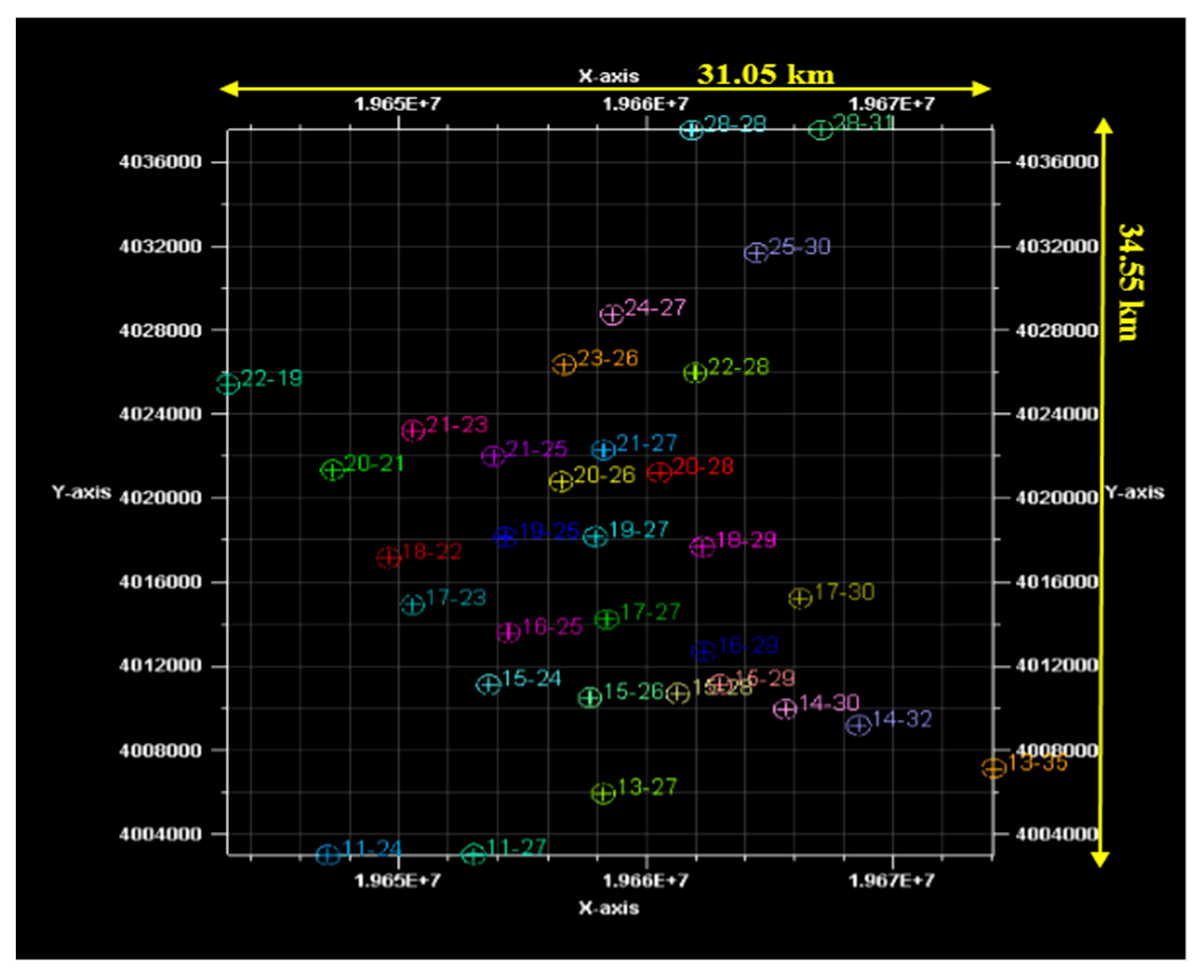
Figure 1.
The drilled wells in the coalbed methane (CBM) gas field from where the seismic data and core samples were retrieved.
Figure 1.
The drilled wells in the coalbed methane (CBM) gas field from where the seismic data and core samples were retrieved.
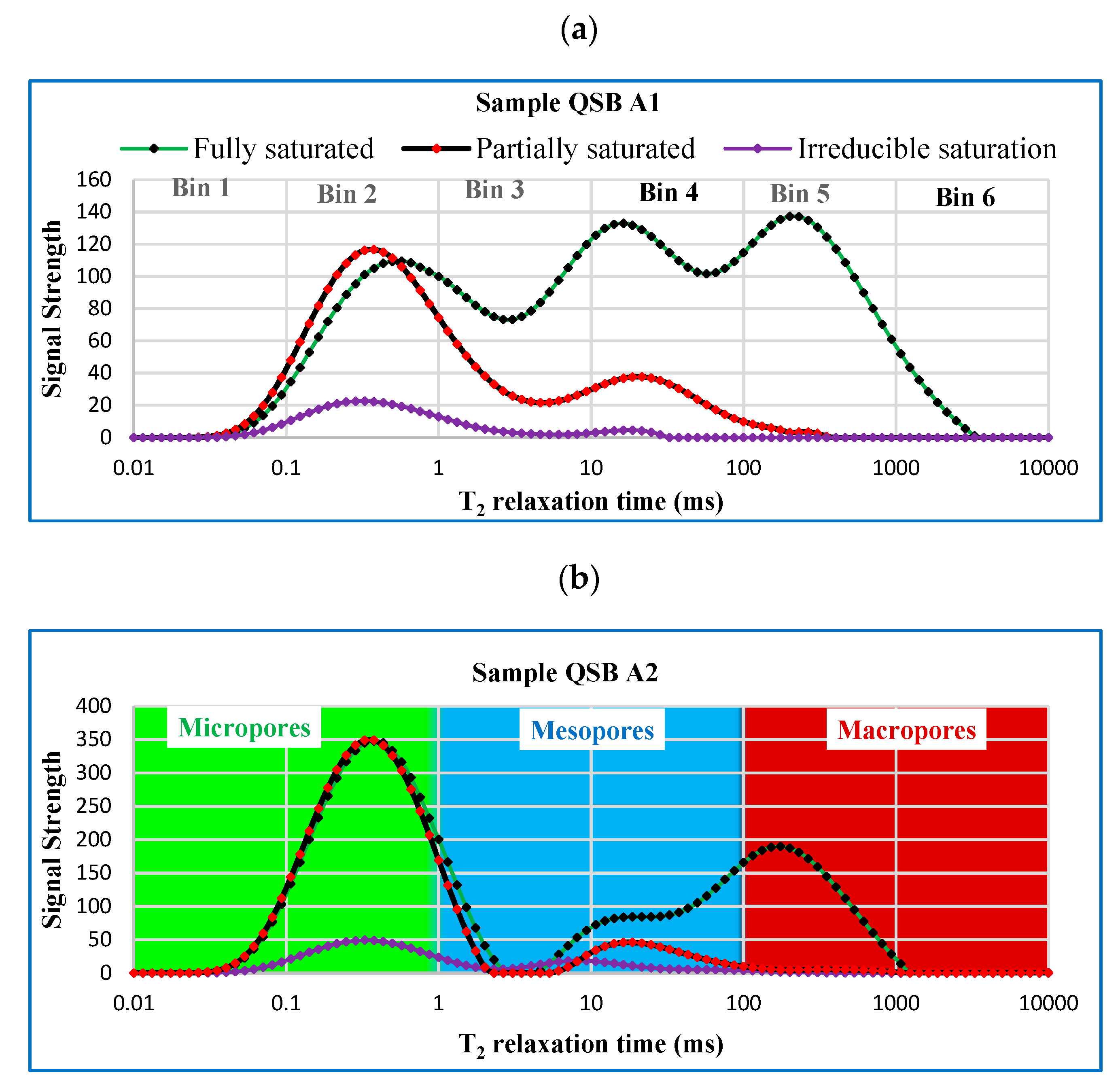
Figure 2.
Nuclear magnetic resonance (NMR) T2 relaxation curves obtained in the laboratory for Sample QSB A1 (a), and Sample QSB A2 (b) under the three states of water saturation, i.e., fully saturated, partially saturated, and irreducible saturation.
Figure 2.
Nuclear magnetic resonance (NMR) T2 relaxation curves obtained in the laboratory for Sample QSB A1 (a), and Sample QSB A2 (b) under the three states of water saturation, i.e., fully saturated, partially saturated, and irreducible saturation.
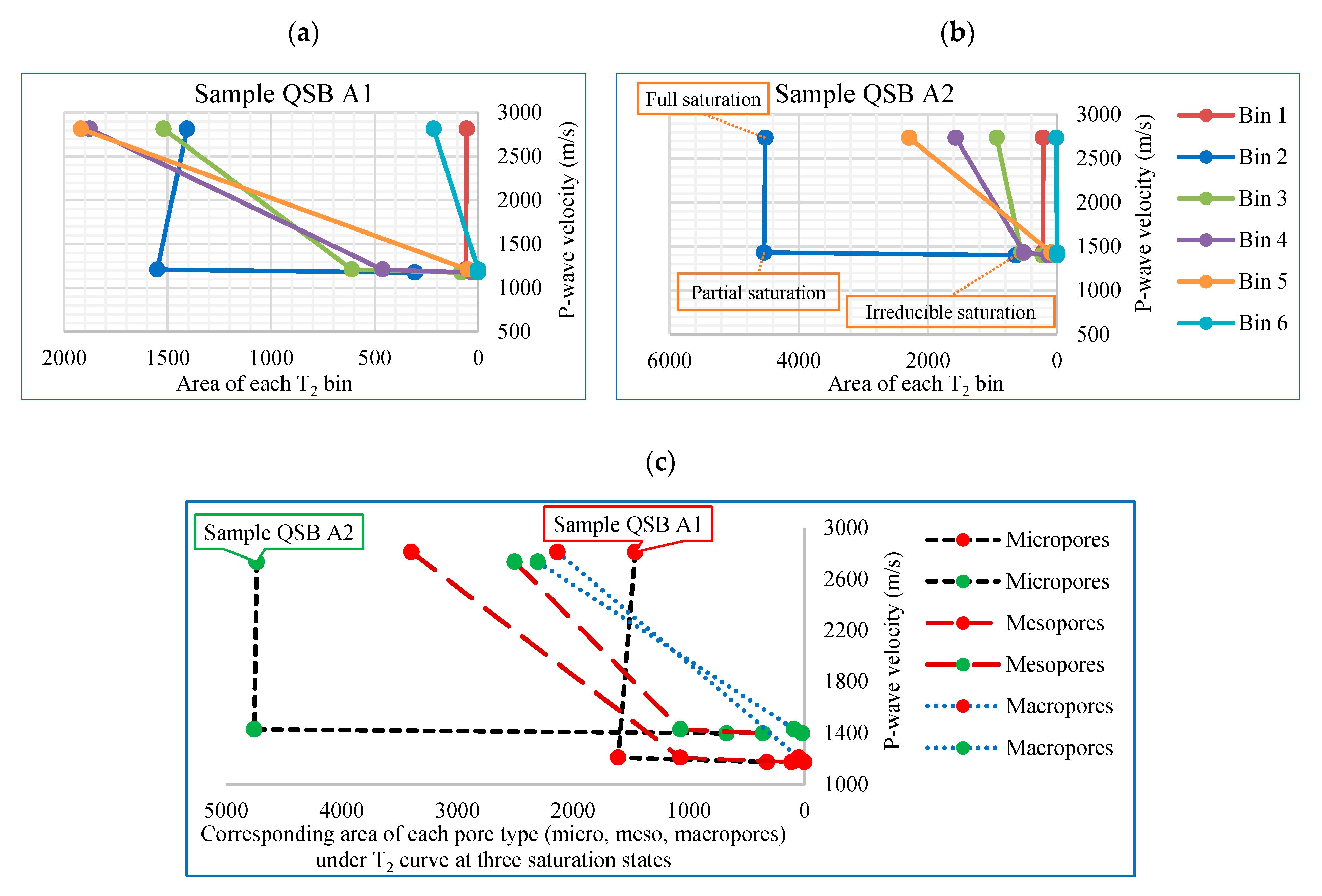
Figure 3.
(a,b) Analyzing the contribution of each pore type (micro, meso, and macropores) to the decrease of elastic P-wave velocity for Sample QSB A1 and Sample QSB A2. The three data points on each graph represent the three saturation states, from left to right: full saturation, partial saturation, and irreducible saturation, respectively; (c) The green and red colors indicate the corresponding data points of the two samples. For each sample, there are three curves, which show the changes of microporosity (black dashed line), mesoporosity (dark red long-dashed line), and macroporosity (blue dotted line) of that sample at three saturation states, from left to right: full saturation, partial saturation, and irreducible saturation, respectively. The porosity value for each pore type at each saturation state was calculated by summing the values of bins 1–2 (for microporosity), bins 3–4 (for mesoporosity), and bins 5–6 (for macroporosity).
Figure 4.
(a) The two studied samples; (b,c) Various pore types, i.e., micro, meso, and macropores inside the Sample QSB A1 and Sample QSB A2, respectively, under the scanning electron microscope. These SEM images only represent the qualitative situation of the internal pore space of the samples and the real bulk porosity was quantitatively measured by the NMR machine.
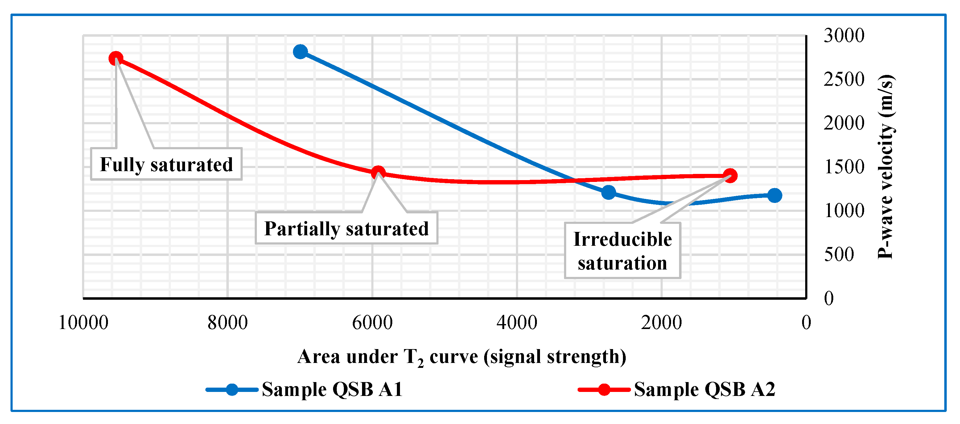
Figure 5.
The relationship between the changes in the elastic and NMR responses of the two coal core samples in the laboratory. Three data points from left to right respectively indicate the fully saturated, partially saturated, and irreducible saturation states.
Figure 5.
The relationship between the changes in the elastic and NMR responses of the two coal core samples in the laboratory. Three data points from left to right respectively indicate the fully saturated, partially saturated, and irreducible saturation states.
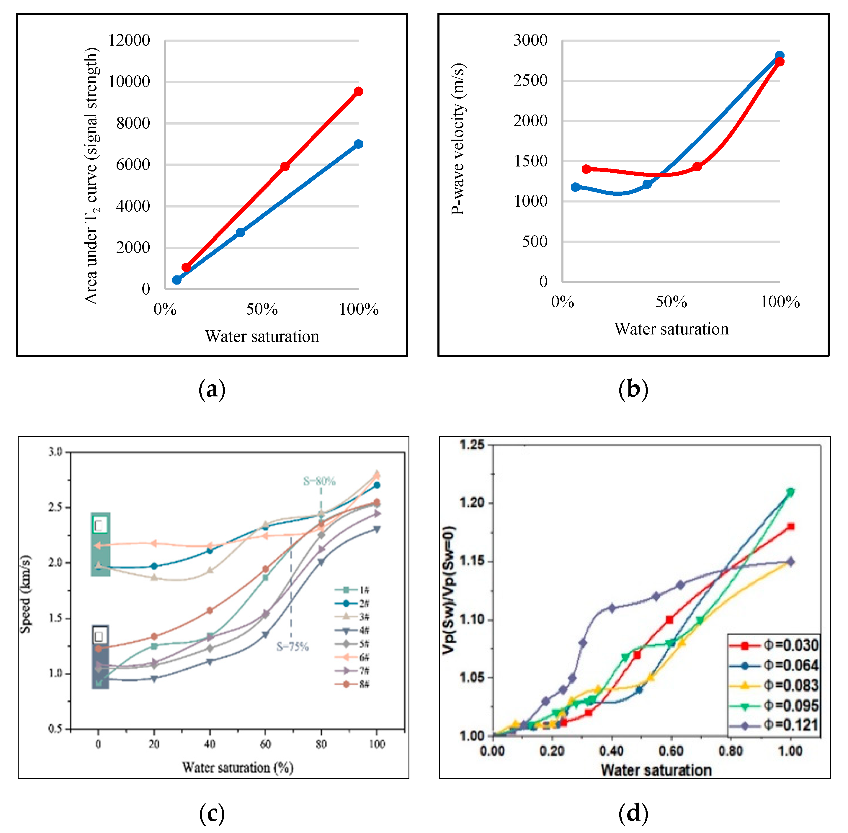
Figure 6.
The relationship between water saturation and area under T
2 curve (
a), and P-wave velocity (
b). Our results were compared with the existing literature: (
c) after [
33] and (
d) after [
43].
Figure 6.
The relationship between water saturation and area under T
2 curve (
a), and P-wave velocity (
b). Our results were compared with the existing literature: (
c) after [
33] and (
d) after [
43].
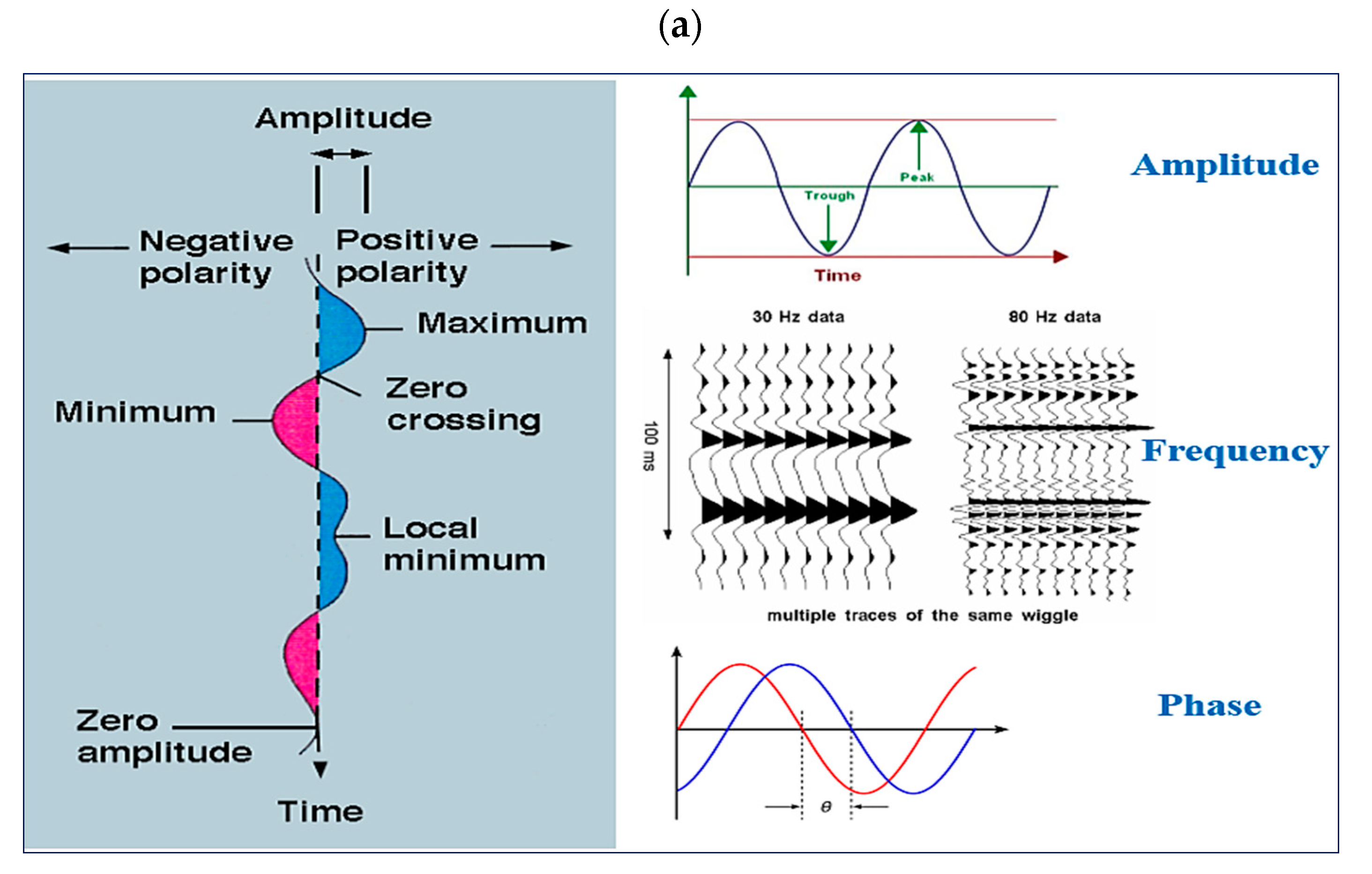
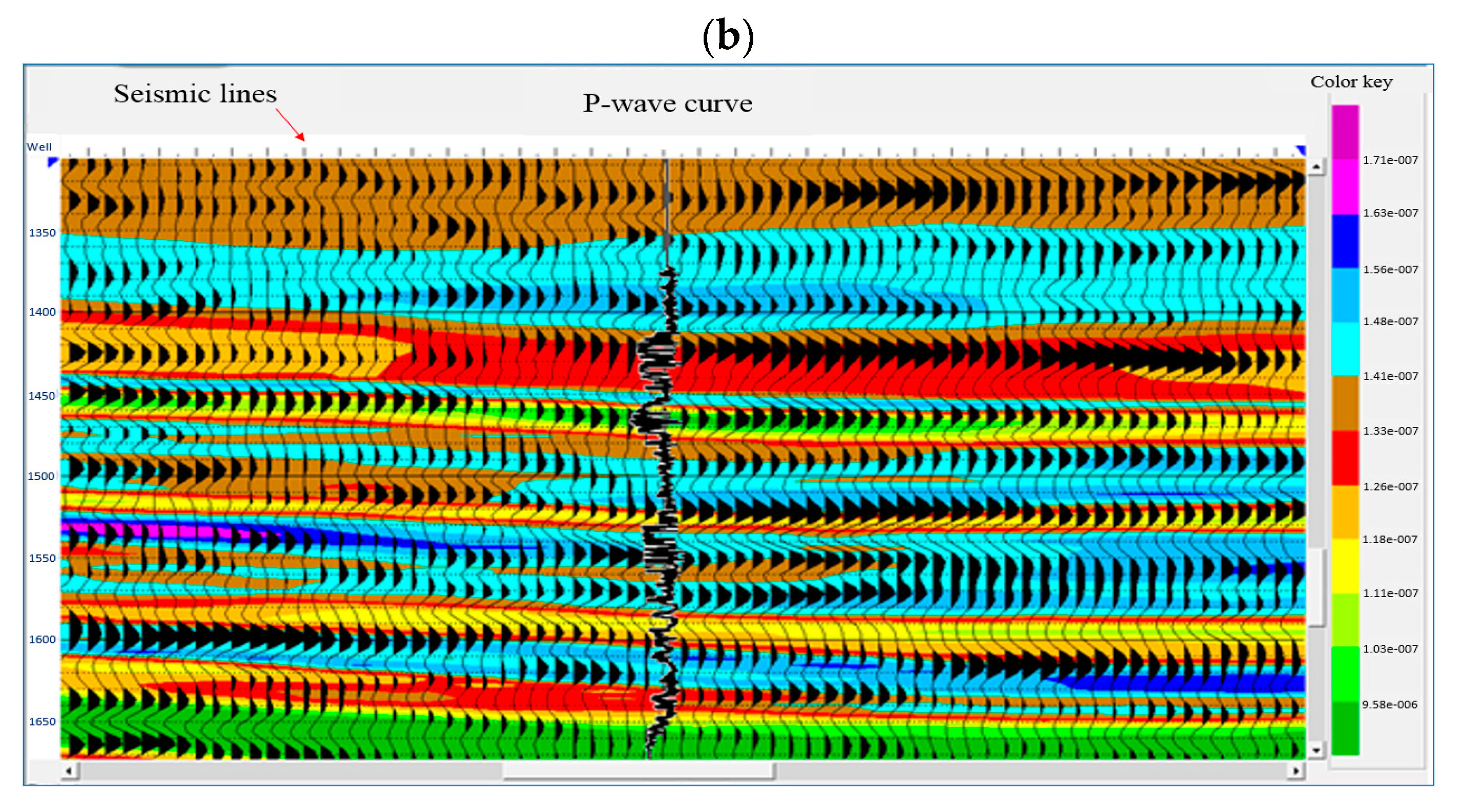
Figure 7.
(a) The most significant components of a seismic trace; (b) Raw seismic data (Wiggle traces) and acoustic impedance inversion (color attribute) in the location of one of the studied wells overlain by the P-wave velocity from logging curve.
Figure 7.
(a) The most significant components of a seismic trace; (b) Raw seismic data (Wiggle traces) and acoustic impedance inversion (color attribute) in the location of one of the studied wells overlain by the P-wave velocity from logging curve.
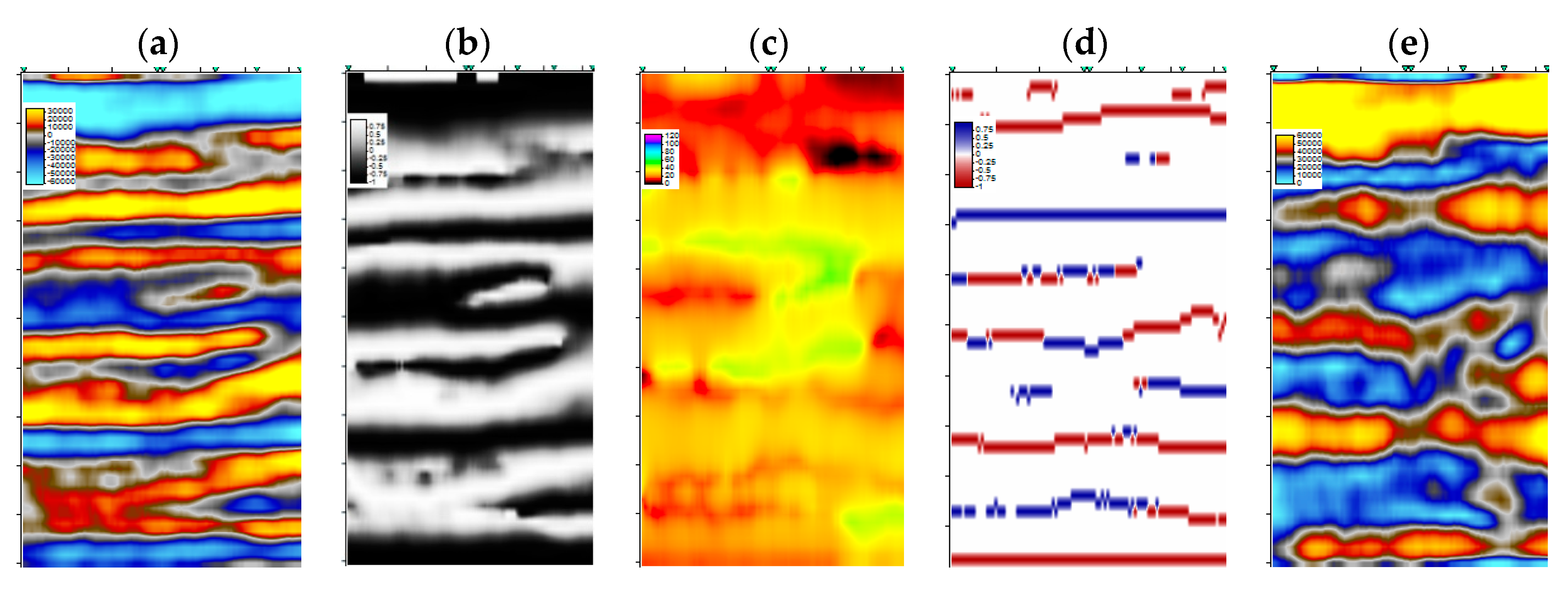
Figure 8.
Two-dimensional (2D) seismic section passing through the employed well (a); and its four corresponding seismic attributes, including cosine of phase (b), instantaneous frequency (c), apparent polarity (d), and amplitude envelope (e).
Figure 8.
Two-dimensional (2D) seismic section passing through the employed well (a); and its four corresponding seismic attributes, including cosine of phase (b), instantaneous frequency (c), apparent polarity (d), and amplitude envelope (e).
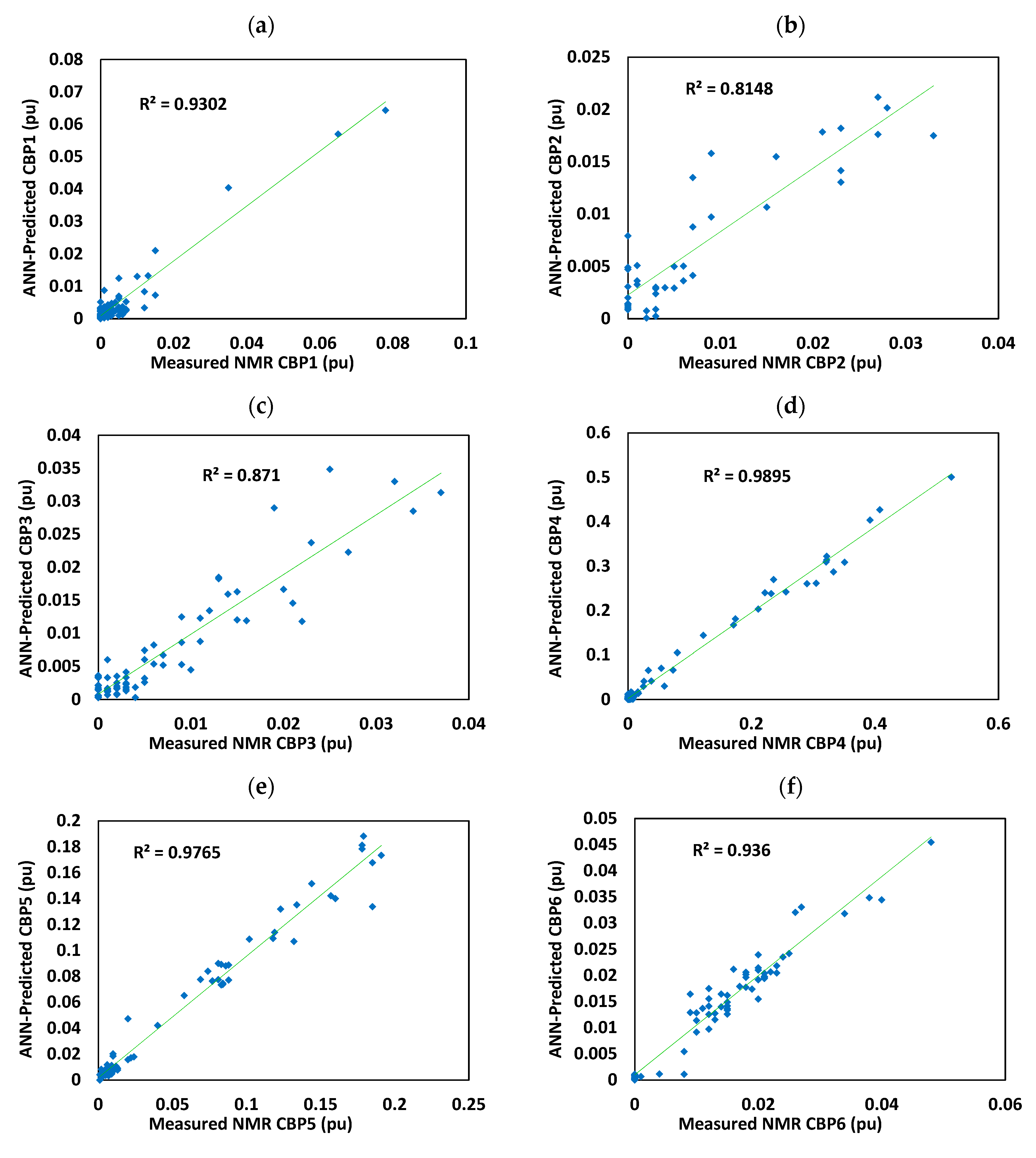
Figure 9.
Correlations of the measured values of bin porosities with the predicted values (pu indicates the porosity unit): (a) CBP1; (b) CBP2; (c) CBP3; (d) CBP4; (e) CBP5; (f) CBP6; (g) CBP7; (h) CBP8.
Figure 9.
Correlations of the measured values of bin porosities with the predicted values (pu indicates the porosity unit): (a) CBP1; (b) CBP2; (c) CBP3; (d) CBP4; (e) CBP5; (f) CBP6; (g) CBP7; (h) CBP8.
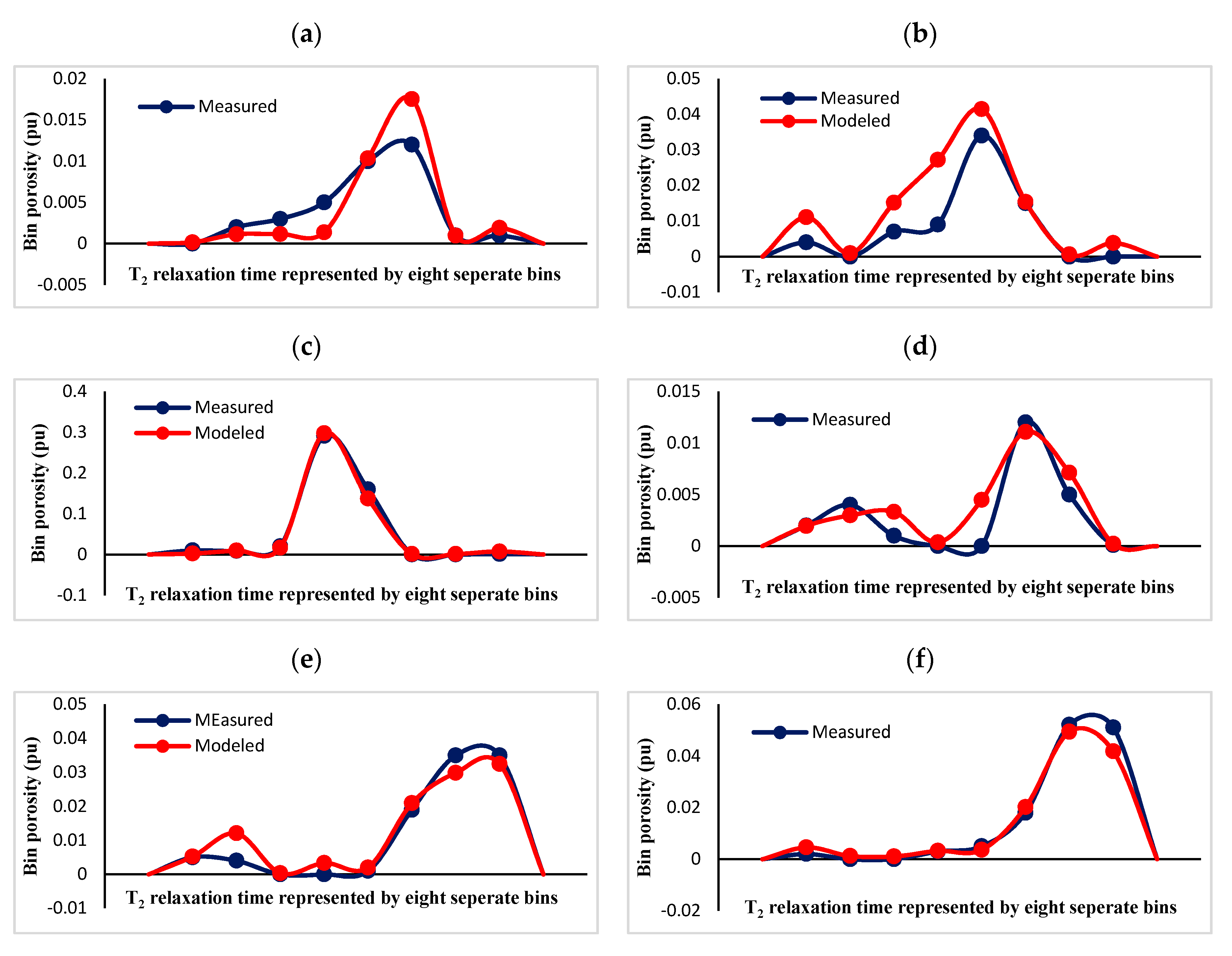
Figure 10.
(a–j) Measured and predicted T2 relaxation curves at ten example points of one studied well. Such relaxation curves could be synthesized for every desired part of the reservoir using the established models and the introduced method.
Figure 10.
(a–j) Measured and predicted T2 relaxation curves at ten example points of one studied well. Such relaxation curves could be synthesized for every desired part of the reservoir using the established models and the introduced method.
Figure 11.
(a,b) The coal formation in the subject CBM gas field from two different views. The thickness of the coal layer is in the range of 2–8.3 m.
Figure 11.
(a,b) The coal formation in the subject CBM gas field from two different views. The thickness of the coal layer is in the range of 2–8.3 m.
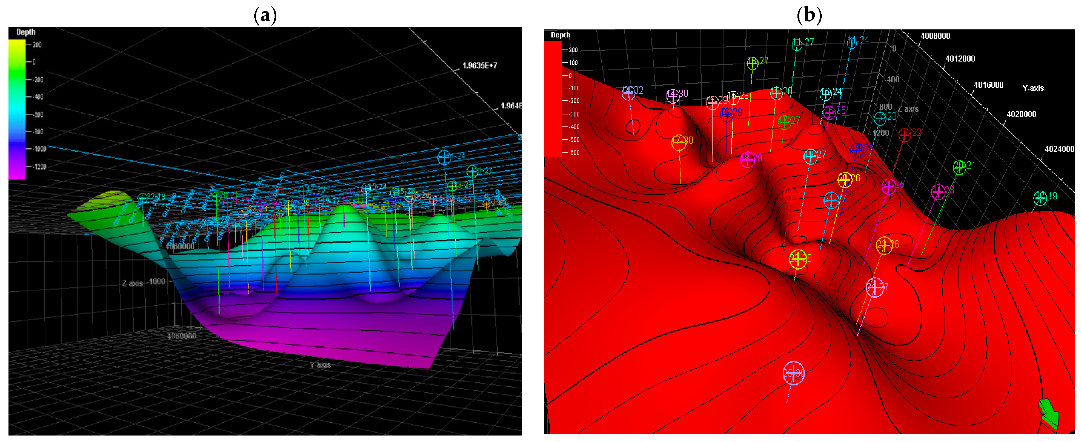
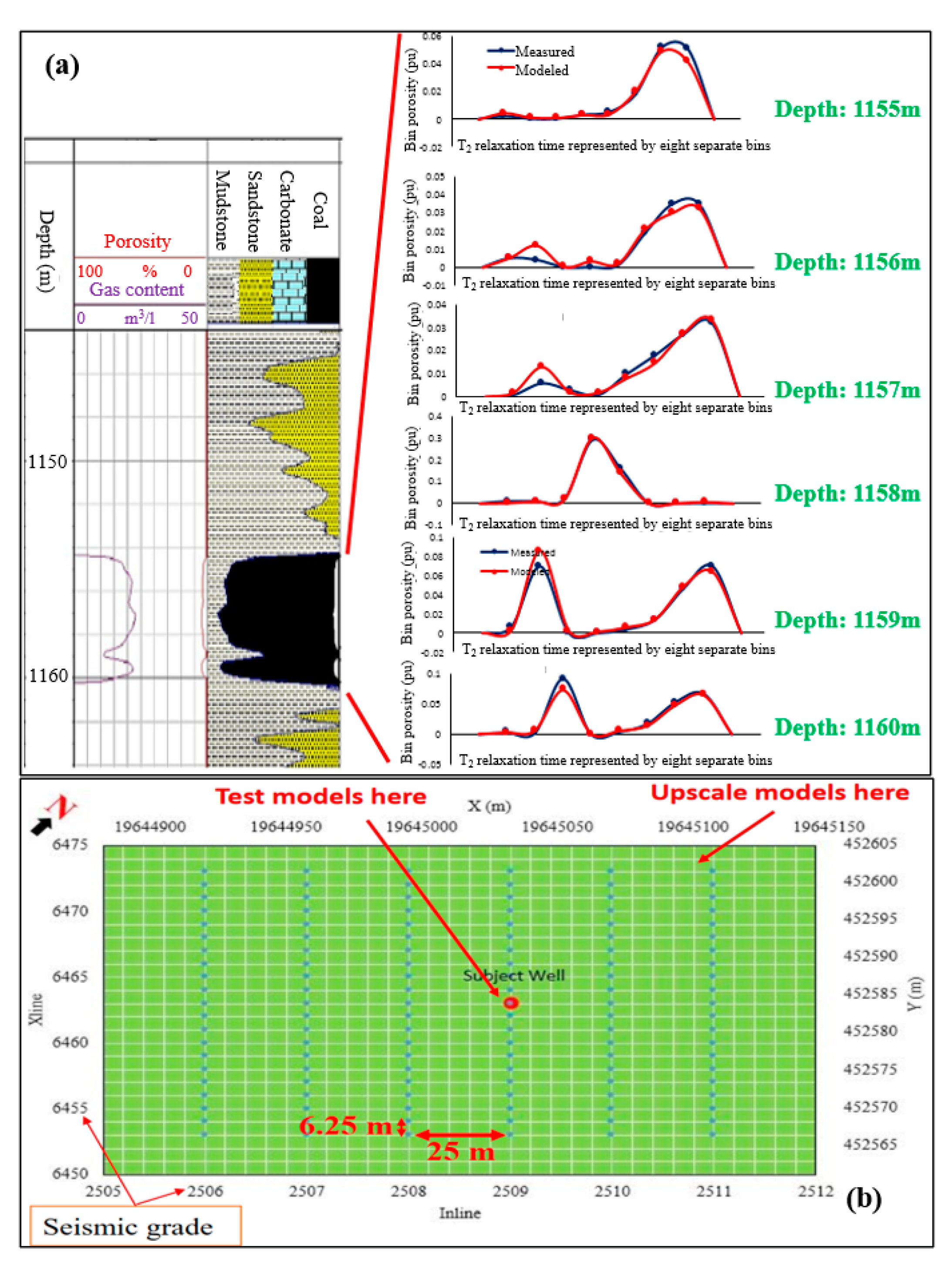
Figure 12.
(a) Predicted T2 curves in the corresponding depths on the well-logging section; (b) Map of the areas and position of the selected simulation nods compared to the subject well. The spacing of the seismic survey inlines and xlines are respectively 25 m and 6.25 m on the map. Therefore, the simulation covered an area of 125 × 125 m2 at the depth of 1157 m.
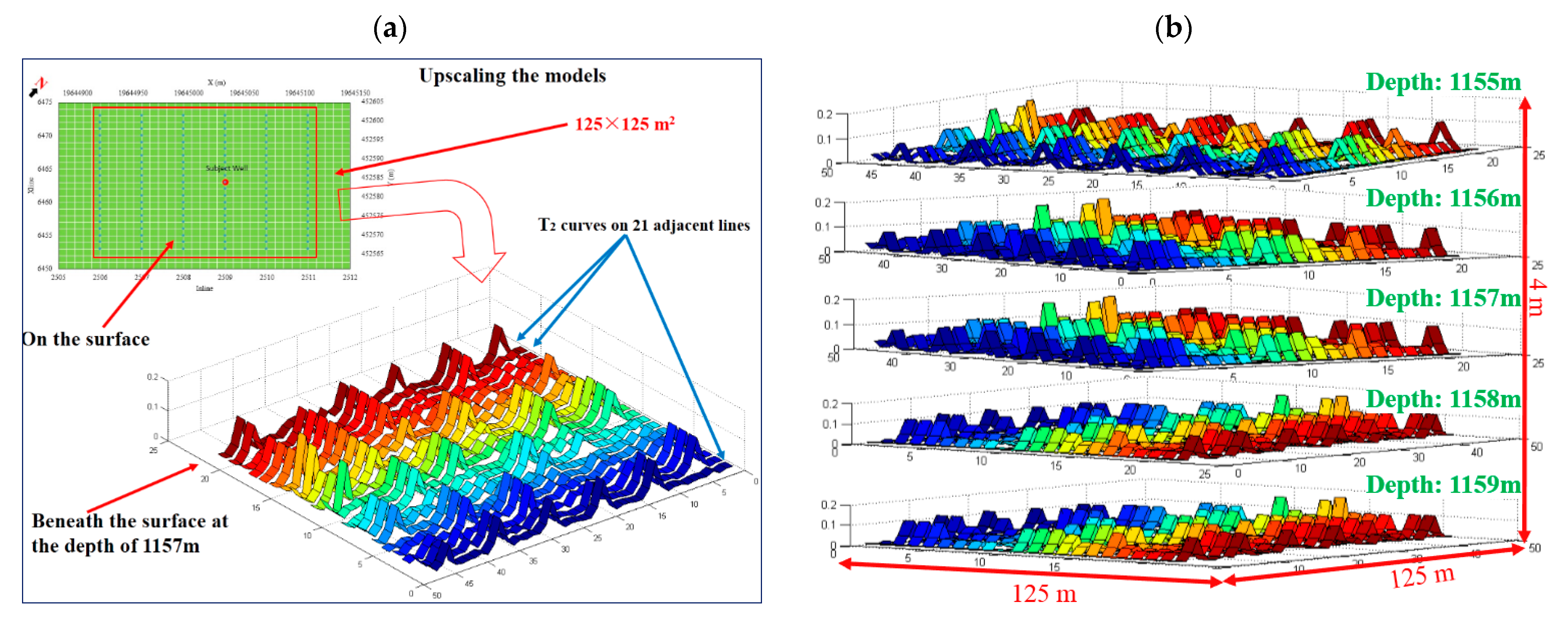
Figure 13.
(a) The finally simulated T2 curves in the depth of 1157 m and their corresponding position on the surface; (b) Simulated T2 curves at various depths of the reservoir which could be estimated for any desired area around the well as far as no considerable geological changes happen.
Figure 13.
(a) The finally simulated T2 curves in the depth of 1157 m and their corresponding position on the surface; (b) Simulated T2 curves at various depths of the reservoir which could be estimated for any desired area around the well as far as no considerable geological changes happen.
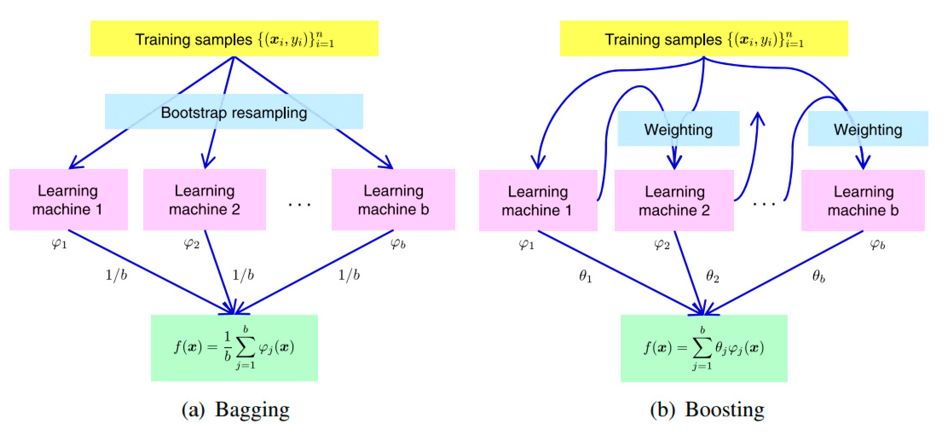
Figure 14.
Ensemble learning. Bagging (
a) trains weak learners in parallel while boosting (
b) trains them sequentially [
53].
Figure 14.
Ensemble learning. Bagging (
a) trains weak learners in parallel while boosting (
b) trains them sequentially [
53].
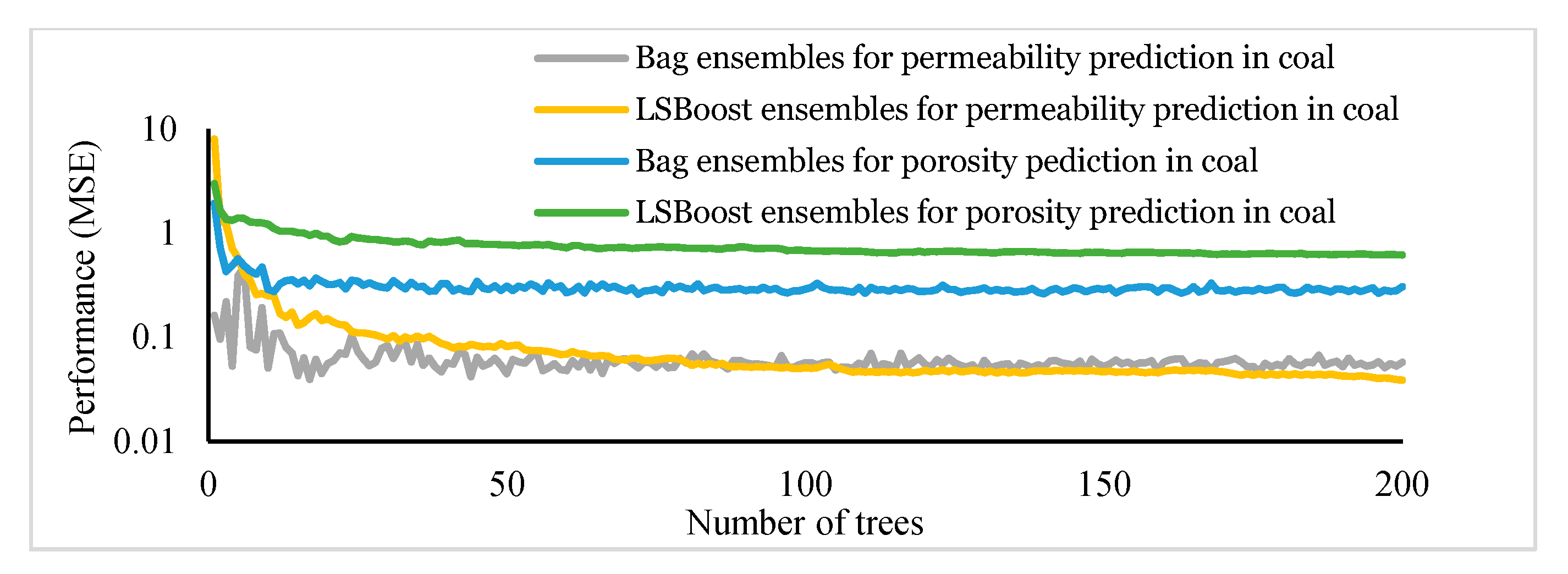
Figure 15.
Prediction error versus the number of trees for statistical ensembles in the studied unconventional coal reservoir.
Figure 15.
Prediction error versus the number of trees for statistical ensembles in the studied unconventional coal reservoir.
Figure 16.
(a) Graphical description of restricted Boltzmann machine (RBM) with n visible and m hidden units; (b) deep belief network (DBN) adopted in the present study with four hidden layers, eight input neurons, and one output neuron.
Figure 16.
(a) Graphical description of restricted Boltzmann machine (RBM) with n visible and m hidden units; (b) deep belief network (DBN) adopted in the present study with four hidden layers, eight input neurons, and one output neuron.
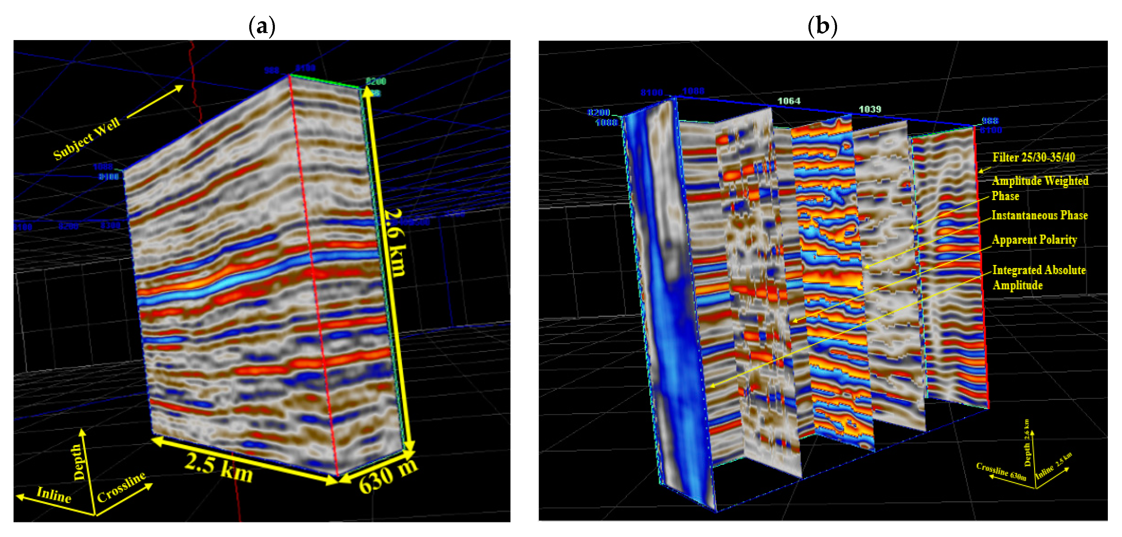
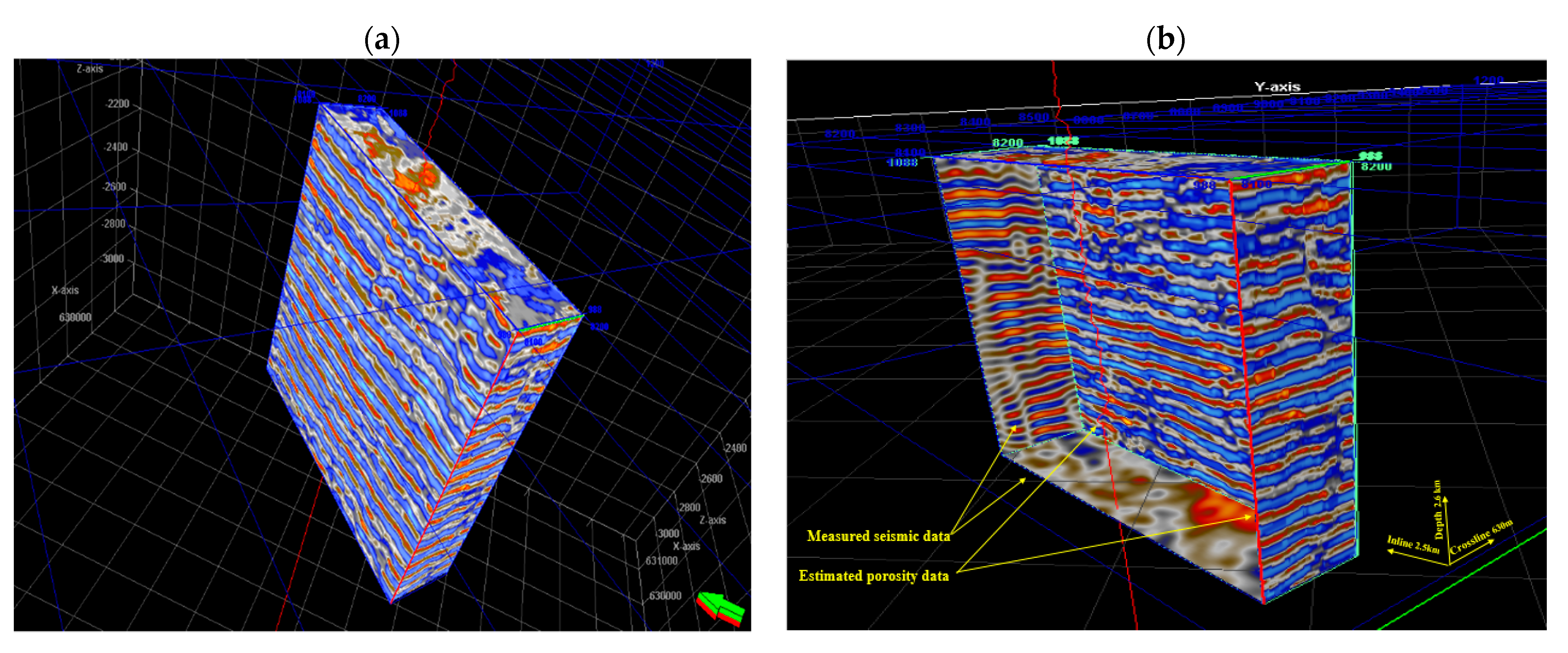
Figure 17.
(a) 3D seismic cube used for extracting the employed attributes at the well location; (b) Employed seismic attributes.
Figure 17.
(a) 3D seismic cube used for extracting the employed attributes at the well location; (b) Employed seismic attributes.
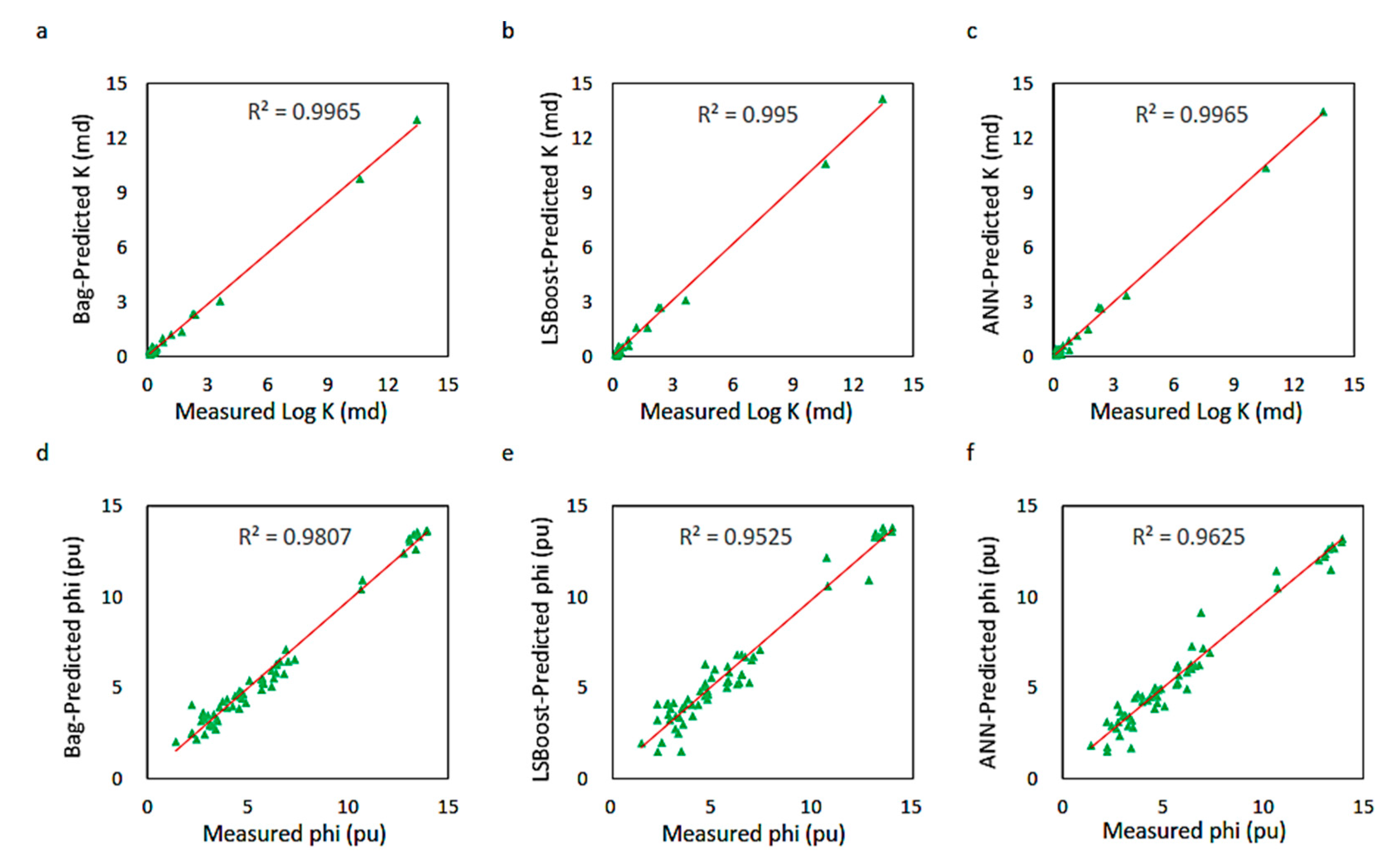
Figure 18.
Correlations of the statistically and intelligently estimated permeability (a–c), and porosity (d–f) with the measured values in the unconventional gas field of the Qinshui Basin of China.
Figure 18.
Correlations of the statistically and intelligently estimated permeability (a–c), and porosity (d–f) with the measured values in the unconventional gas field of the Qinshui Basin of China.
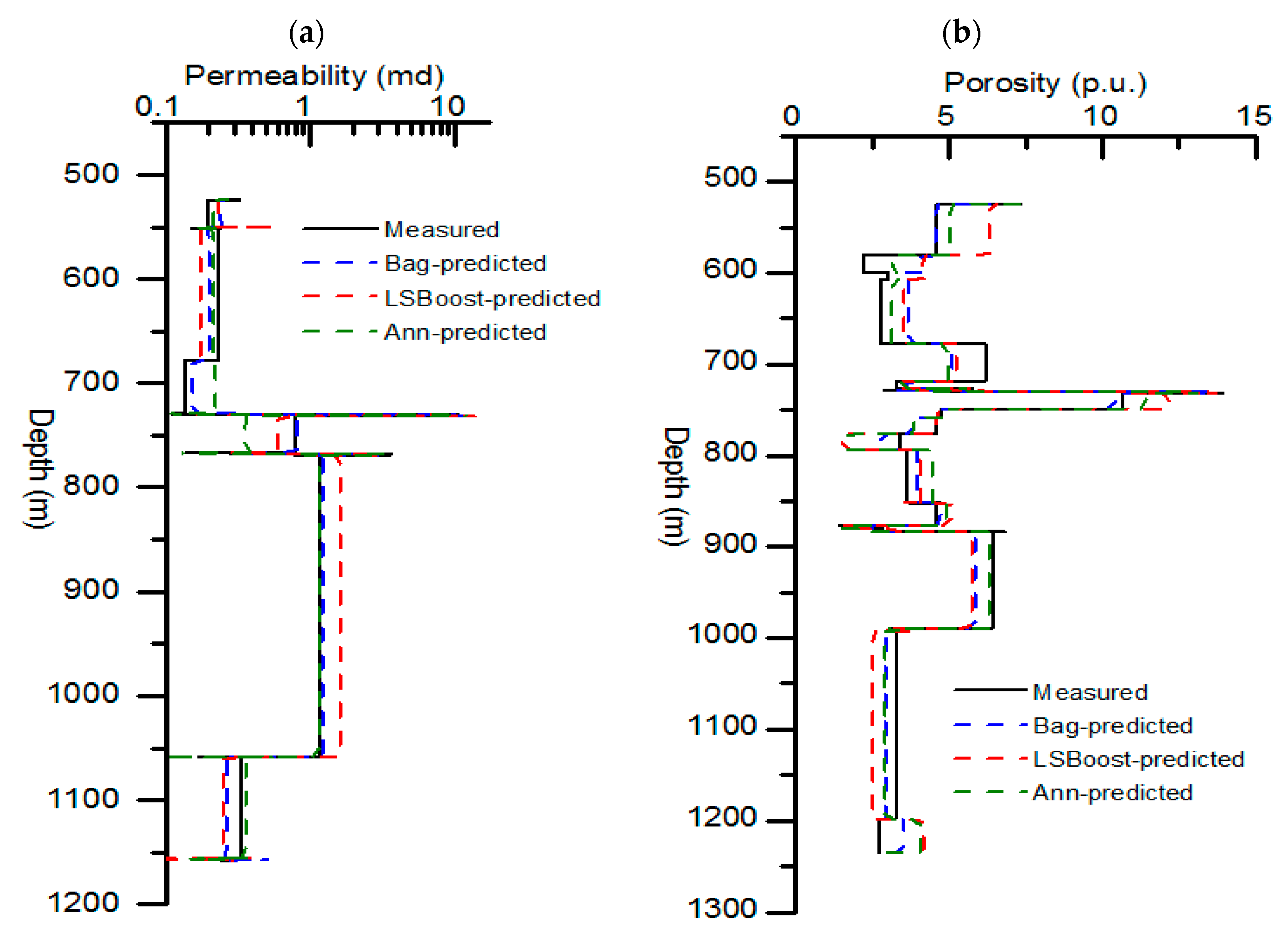
Figure 19.
Measured (black), Bag-predicted (blue), LSBoost-predicted (red), and deep learning-predicted (green) curves of permeability (a) and porosity (b) in the unconventional coal reservoir. The stepped representation provides the comparison among the average permeability at different sections of the well, i.e., low permeable and highly permeable sections.
Figure 20.
(a) 3D porosity cube around one of the subject wells estimated using the statistical Bag ensemble; (b) Evaluation of the estimated porosity cube (right, front, and surface walls) using a measured 3D seismic attribute, i.e., frequency filter. The satisfying agreement of the statistical model’s result with the measured data proves the reliability of the technique.
Table 1.
The results of the laboratory measurements of the elastic and magnetic resonance responses of the coal samples at three states of fully saturated, partially saturated, and irreducible saturation.
Table 1.
The results of the laboratory measurements of the elastic and magnetic resonance responses of the coal samples at three states of fully saturated, partially saturated, and irreducible saturation.
| | Sample QSB A1 | Sample QSB A2 |
|---|
| | Fully Saturated | Partially Saturated | Irreducible Saturation | Fully Saturated | Partially Saturated | Irreducible Saturation |
|---|
| Bin 1 | 54.83 | 59.04 | 17.76 | 216.22 | 220.74 | 34.31 |
| Bin 2 | 1407.12 | 1550.77 | 305.33 | 4518.45 | 4534.76 | 637.77 |
| Bin 3 | 1520.36 | 610.10 | 81.81 | 934.53 | 555.25 | 221.21 |
| Bin 4 | 1877.52 | 462.29 | 29.38 | 1569.87 | 516.82 | 135.66 |
| Bin 5 | 1919.41 | 49.09 | 0.00 | 2290.21 | 88.20 | 19.95 |
| Bin 6 | 214.95 | 0.00 | 0.00 | 14.12 | 1.68 | 0.00 |
| VP (m/s) | 2813.14 | 1209.59 | 1174.65 | 2735 | 1430.45 | 1398.60 |
| Bins summed | 6994.19 | 2731.29 | 434.28 | 9543.4 | 5917.45 | 1048.9 |
| Decrease in the overall bin area | - | −4262.9 | −2297.01 | - | −3625.95 | −4868.55 |
| Saturation | 100% | 39% | 6% | 100% | 62% | 11% |
| Decrease in VP (m/s) | - | −1603.55 | −34.94 | - | −1304.55 | −31.85 |
Table 2.
A brief explanation of the most important seismic attributes employed in the current study [
50].
Table 2.
A brief explanation of the most important seismic attributes employed in the current study [
50].
| Instantaneous Frequency | Instantaneous frequency is the time derivative of the phase. This attribute should not be confused with the frequency of the wavelet. It is often used to estimate seismic attenuation. Oil and gas reservoirs usually cause drop-off of high-frequency components. It helps to measure cyclicity of geological intervals and can be useful for cross-correlation across faults. It could also identify contacts between gas and water or gas and oil. Instantaneous frequency tends to be unstable in the presence of noise and is sometimes difficult to interpret. This attribute is calculated as: |
| Instantaneous Phase | The attribute is calculated on a sample by sample basis without regard of the waveform. The attribute provides an amplitude independent display. It is commonly used to find continuity of weak events and to distinguish small faults and dipping events.
Instantaneous phase is calculated as: |
| Frequency Filter | The frequency-filter attribute is useful for enhancing particular seismic events or to reduce unwanted noise in the data. This can improve the accuracy of interpretation. |
| Apparent Polarity | The polarity of the instantaneous phase, calculated at the local amplitude extreme. The apparent polarity reveals the sign of the reflection coefficient and therefore indicates features that would change it, e.g., unconformities. It is useful for checking the lateral variation of polarity along a reflection layer. On a noisy seismic section, event continuity can be clearer on the apparent polarity than the original seismic section. This attribute reveals reflection details without the waveform effects and can help detect thick beds when the data is of good quality (less noise). |
| Amplitude Envelope | The total instantaneous energy of the analytic signal (the complex trace), independent of phase, calculated as: where f and g are the “real” and “imaginary” components of the seismic trace. So, if f is the real part, which are just the original seismic trace samples, g will be the samples from the Hilbert transform (also called quadrature amplitude) of the seismic trace. |
| Relative Acoustic Impedance | Relative acoustic impedance is a running sum of regularly sampled amplitude values. This attribute is calculated by integrating the seismic trace and passing the result through a high-pass Butterworth filter with a hard-coded cut-off at (10*sample rate) Hz. |
| Reflection Intensity | Reflection Intensity is the average amplitude over a specified window (9 samples in the present study) multiplied with the sample interval. Reflection Intensity is useful for the delineation of amplitude features while retaining the frequency appearance of the original seismic data. |
| RMS Amplitude | RMS amplitude is the square root of the sum of the squared amplitudes divided by the number of live samples as shown in the following formula: |
| Second Derivative | The second time derivative of the input seismic volume. The combination of the original amplitude, first derivative, and second derivative allows you to express seismic interpretation in relationship to maximum, minimums, greatest descents, and descent polarity. The second derivative can be used to help guide the pick by providing continuity in areas of where reflections are poorly resolved on the raw amplitude. Lateral amplitude variations are visibly diminished, which will make auto-tracking regional events more difficult. |
Table 3.
Linear relationships of the seismic attributes (inputs) and CBPs (outputs)
Table 3.
Linear relationships of the seismic attributes (inputs) and CBPs (outputs)
| CBP1 | Attribute | R2 | CBP2 | Attribute | R2 |
| Derivative Instantaneous Amplitude | 0.1315 | Inversion | 0.1236 |
| Squared Inverted Inversion | 0.1320 | Derivative Instantaneous Amplitude | 0.1070 |
| TWT | 0.1586 | Frequency Filter | 0.1650 |
| Frequency Filter | 0.2018 | Instantaneous Phase | 0.1112 |
| Amplitude Weighted Cosine Phase | 0.1341 | TWT | 0.1446 |
| CBP3 | Squared Inversion | 0.2728 | CBP4 | Amplitude Weighted Cosine Phase | 0.2302 |
| Cosine Instantaneous Phase | 0.3860 | Instantaneous Frequency | 0.2745 |
| Seismic Amplitudes | 0.4238 | Frequency Filter | 0.4918 |
| Amplitude Weighted Cosine Phase | 0.3140 | Cosine Instantaneous Phase | 0.5503 |
| Amplitude Integrate | 0.3130 | Seismic Amplitudes | 0.6225 |
| CBP5 | Amplitude Weighted Cosine Phase | 0.3602 | CBP6 | Instantaneous Frequency | 0.4461 |
| TWT | 0.3655 | Frequency Filter | 0.5483 |
| Squared Inversion | 0.4747 | Amplitude Weighted Phase | 0.4575 |
| Cosine Instantaneous Phase | 0.5098 | Cosine Instantaneous Phase | 0.4182 |
| Seismic Amplitudes | 0.5747 | Seismic Amplitudes | 0.4654 |
| CBP7 | Derivative Instantaneous Amplitude | 0.4885 | CBP8 | Amplitude Weighted Cosine Phase | 0.3428 |
| Inverted Inversion | 0.7804 | Derivative Instantaneous Amplitude | 0.3969 |
| Amplitude Integrate | 0.6728 | Inverted Inversion | 0.7129 |
| Amplitude Weighted Cosine Phase | 0.4530 | TWT | 0.5693 |
| TWT | 0.7173 | Integrated Absolute Amplitude | 0.1402 |
Table 4.
Properties of the training data and performance of the intelligent models.
Table 4.
Properties of the training data and performance of the intelligent models.
| Target Curve | CBP1 | CBP2 | CBP3 | CBP4 | CBP5 | CBP6 | CBP7 | CBP8 |
|---|
| No. of input attributes | 5 | 5 | 5 | 5 | 5 | 5 | 5 | 5 |
| Total No. of available data pairs | 520 | 277 | 476 | 536 | 545 | 431 | 503 | 568 |
| No. of training and validation data | 442 | 235 | 405 | 456 | 463 | 366 | 428 | 483 |
| No. of test data | 78 | 42 | 71 | 80 | 82 | 65 | 75 | 85 |
| No. of neurons in hidden layers | 30 | 30 | 30 | 30 | 30 | 30 | 30 | 30 |
| Iteration the best ANN model was achieved | 321 | 203 | 311 | 260 | 288 | 346 | 198 | 169 |
| Performance of the ANN model (MSE) | 1.12 × 10⁻⁵ | 2.27 × 10⁻⁵ | 1.05 × 10⁻⁵ | 1.80 × 10⁻⁴ | 8.41 × 10⁻⁵ | 7.06 × 10⁻⁶ | 6.92 × 10⁻⁶ | 2.29 × 10⁻⁵ |
| Correlation with measured data (R2) | 0.93 | 0.81 | 0.88 | 0.99 | 0.98 | 0.94 | 0.98 | 0.94 |
Table 5.
Comparison between the performance of various ANN training algorithms for bins 1 and 2.
Table 5.
Comparison between the performance of various ANN training algorithms for bins 1 and 2.
| | Modeled Parameter | CBP1 | CBP2 |
|---|
| Training Algorithm | | R2 | MSE | R2 | MSE |
|---|
| conjugate gradient with Powell/Beale restarts (CGB) | 0.73 | 7.19 × 10⁻⁵ | 0.67 | 6.95 × 10⁻⁵ |
| back-propagation with adaptive learning rate (GDA) | 0.67 | 9.49 × 10⁻⁵ | 0.66 | 5.32 × 10⁻⁵ |
| Levenberg–Marquardt (LM) | 0.93 | 1.12 × 10⁻⁵ | 0.81 | 2.27 × 10⁻⁵ |
| one step secant (OSS) | 0.63 | 1.35 × 10⁻⁴ | 0.71 | 1.70 × 10⁻⁵ |
| resilient back-propagation (RP) | 0.62 | 9.21 × 10⁻⁵ | 0.66 | 3.43 × 10⁻⁵ |
| scaled conjugate gradient (SCG) | 0.76 | 4.65 × 10⁻⁵ | 0.69 | 3.12 × 10⁻⁵ |
Table 6.
Comparison between the performance of various ANN training algorithms for bins 3 and 4.
Table 6.
Comparison between the performance of various ANN training algorithms for bins 3 and 4.
| | Modeled Parameter | CBP3 | CBP4 |
|---|
| Training Algorithm | | R2 | MSE | R2 | MSE |
|---|
| conjugate gradient with Powell/Beale restarts (CGB) | 0.78 | 2.60 × 10⁻⁵ | 0.94 | 1.60 × 10⁻³ |
| back-propagation with adaptive learning rate (GDA) | 0.71 | 1.52 × 10⁻⁵ | 0.87 | 3.20 × 10⁻³ |
| Levenberg–Marquardt (LM) | 0.88 | 1.05 × 10⁻⁵ | 0.99 | 2.00 × 10⁻⁴ |
| one step secant (OSS) | 0.79 | 2.64 × 10⁻⁵ | 0.92 | 1.20 × 10⁻³ |
| resilient back-propagation (RP) | 0.76 | 3.02 × 10⁻⁵ | 0.88 | 3.00 × 10⁻³ |
| scaled conjugate gradient (SCG) | 0.83 | 3.66 × 10⁻⁵ | 0.94 | 1.50 × 10⁻³ |
Table 7.
Comparison between the performance of various ANN training algorithms for bins 5 and 6.
Table 7.
Comparison between the performance of various ANN training algorithms for bins 5 and 6.
| | Modeled Parameter | CBP5 | CBP6 |
|---|
| Training Algorithm | | R2 | MSE | R2 | MSE |
|---|
| conjugate gradient with Powell/Beale restarts (CGB) | 0.94 | 2.93 × 10⁻⁴ | 0.91 | 1.12 × 10⁻⁵ |
| back-propagation with adaptive learning rate (GDA) | 0.93 | 2.85 × 10⁻⁴ | 0.83 | 3.17 × 10⁻⁵ |
| Levenberg–Marquardt (LM) | 0.98 | 8.41 × 10⁻⁵ | 0.94 | 7.06 × 10⁻⁵ |
| one step secant (OSS) | 0.93 | 3.14 × 10⁻⁴ | 0.84 | 2.09 × 10⁻⁵ |
| resilient back-propagation (RP) | 0.91 | 3.99 × 10⁻⁴ | 0.88 | 1.49 × 10⁻⁵ |
| scaled conjugate gradient (SCG) | 0.92 | 2.62 × 10⁻⁴ | 0.90 | 1.39 × 10⁻⁵ |
Table 8.
Comparison between the performance of various ANN training algorithms for bins 7 and 8.
Table 8.
Comparison between the performance of various ANN training algorithms for bins 7 and 8.
| | Modeled Parameter | CBP7 | CBP8 |
|---|
| Training Algorithm | | R2 | MSE | R2 | MSE |
|---|
| conjugate gradient with Powell/Beale restarts (CGB) | 0.95 | 1.54 × 10⁻⁵ | 0.90 | 4.04 × 10⁻⁵ |
| back-propagation with adaptive learning rate (GDA) | 0.95 | 1.49 × 10⁻⁵ | 0.90 | 4.11 × 10⁻⁵ |
| Levenberg–Marquardt (LM) | 0.98 | 6.92 × 10⁻⁶ | 0.94 | 2.29 × 10⁻⁵ |
| one step secant (OSS) | 0.94 | 1.90 × 10⁻⁵ | 0.91 | 4.14 × 10⁻⁵ |
| resilient back-propagation (RP) | 0.93 | 1.95 × 10⁻⁵ | 0.90 | 4.23 × 10⁻⁵ |
| scaled conjugate gradient (SCG) | 0.95 | 1.62 × 10⁻⁵ | 0.92 | 4.20 × 10⁻⁵ |
Table 9.
The selected input attributes for estimating permeability and porosity.
Table 9.
The selected input attributes for estimating permeability and porosity.
| Permeability | | Porosity | |
|---|
| Attribute | R2 | Attribute | R2 |
|---|
| Amplitude Envelope | 0.4160 | Amplitude Envelope | 0.5872 |
| RMS Amplitude | 0.4639 | RMS Amplitude | 0.5826 |
| Integrated Absolute Amplitude | 0.3369 | Integrated Absolute Amplitude | 0.5497 |
| Filter 25/30–35–40 | 0.5240 | Filter 25/30–35–40 | 0.6121 |
| Reflection Intensity | 0.5142 | Reflection Intensity | 0.5614 |
| Instantaneous Phase | 0.3701 | Instantaneous Phase | 0.5947 |
| Derivative Instantaneous Amplitude | 0.4669 | Relative Acoustic Impedance | 0.4433 |
| Cosine Instantaneous Phase | 0.7454 | Instantaneous Frequency | 0.2635 |
Table 10.
Properties of the employed data pairs for estimating petrophysical properties from the seismic attributes by both statistical and deep learning models.
Table 10.
Properties of the employed data pairs for estimating petrophysical properties from the seismic attributes by both statistical and deep learning models.
| Target Curve | Permeability | Porosity |
|---|
| Number of input variables | 8 | 8 |
| Total No. of available data pairs | 231 | 355 |
| No. of training data | 185 | 295 |
| No. of test data | 46 | 60 |
| No. of neurons in the hidden layer | 20 | 20 |
| Iteration the best ANN model was achieved | 265 | 94 |
| Optimal number of trees for statistical Bag ensembles | 17 | 72 |
| Optimal number of trees for statistical LSBoost ensembles | 200 | 200 |
Table 11.
Performance of the employed algorithms in estimating petrophysical properties from the post-stack seismic data.
Table 11.
Performance of the employed algorithms in estimating petrophysical properties from the post-stack seismic data.
| Target NMR Curve | Permeability | Porosity |
|---|
| Model Performance | MSE | R2 | MSE | R2 |
|---|
| Bag ensemble | 3.95 × 10⁻² | 0.9965 | 2.59 × 10⁻¹ | 0.9807 |
| LSBoost ensemble | 3.89 × 10⁻² | 0.9950 | 6.19 × 10⁻¹ | 0.9525 |
| Artificial neural network | 2.13 × 10⁻² | 0.9965 | 5.20 × 10⁻¹ | 0.9625 |


 ,
, 


