
Deep-Learning Forecasting Method for Electric Power Load via Attention-Based Encoder-Decoder with Bayesian Optimization

 ,
,  , ,
, ,
Abstract
:1. Introduction
- (1)
- Improve the prediction model’s overall performance for electrical load by designing appropriate GRU-based encoder-decoder architecture incorporating temporal attention mechanism, adjusting the non-linear degree and dynamic adaptability of the network.
- (2)
- Replace the previous manually selected ways, the Bayesian optimization algorithm is utilized to automatically assure the hyperparameters of encoder-decoder model, which results in improving prediction performance and training efficiency of seq2seq method with too many parameters.
2. Materials and Methods
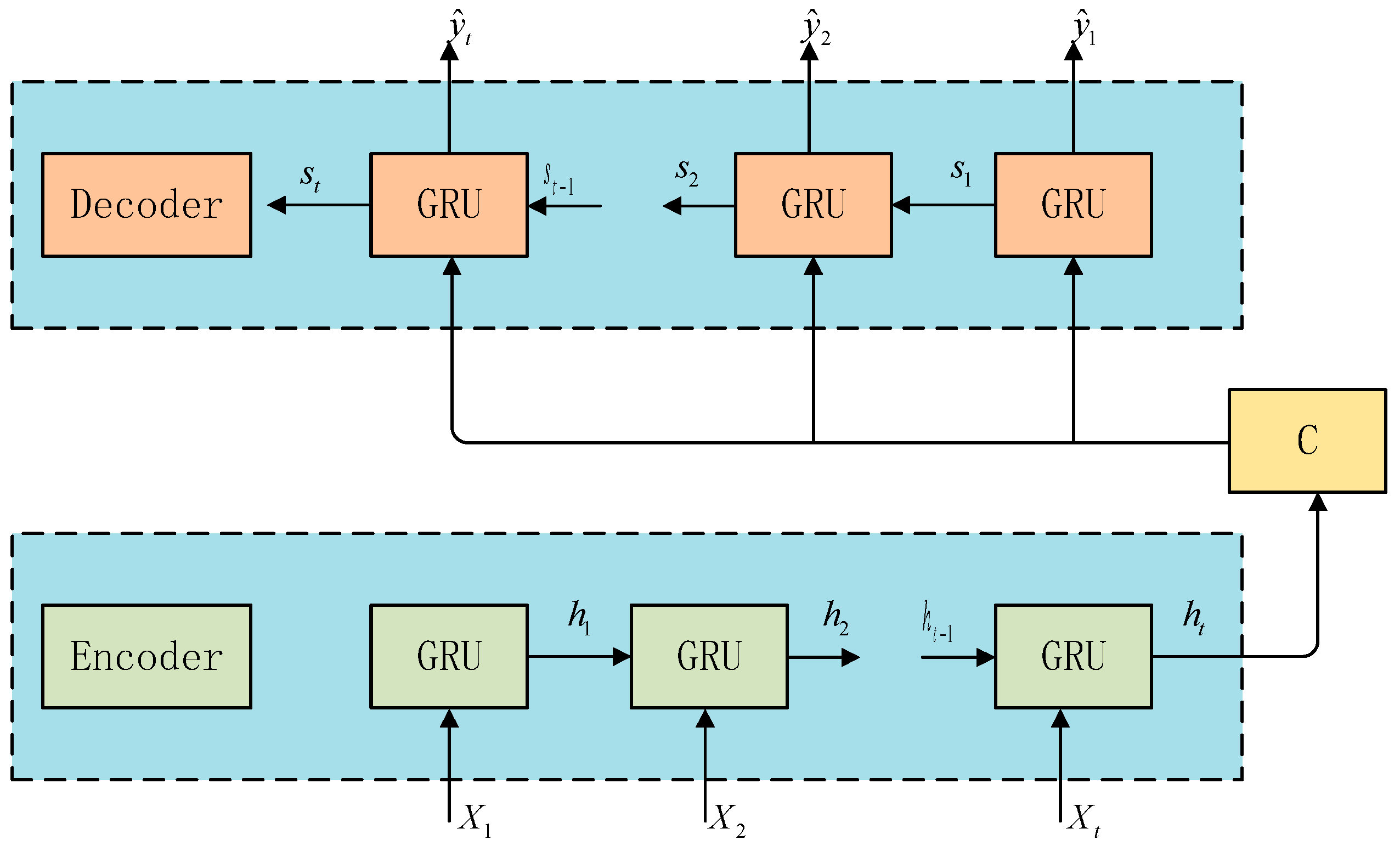
2.1. Traditional Encoder-Decoder Structure
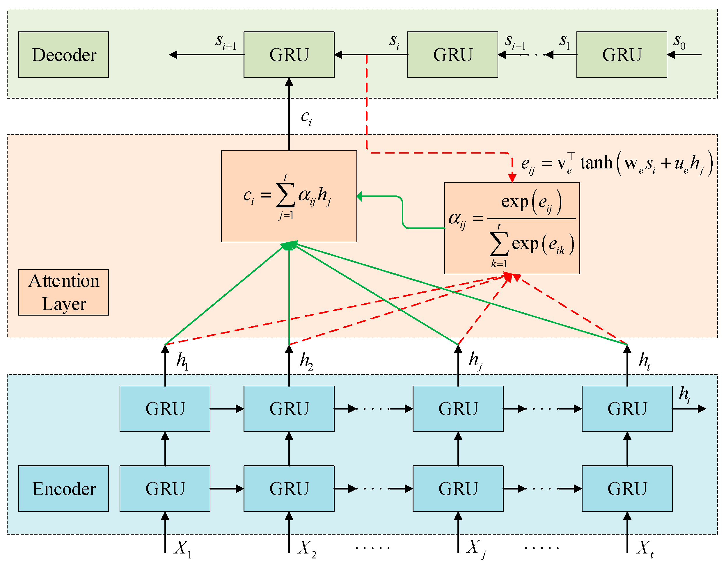
2.2. Temporal Attention Layer
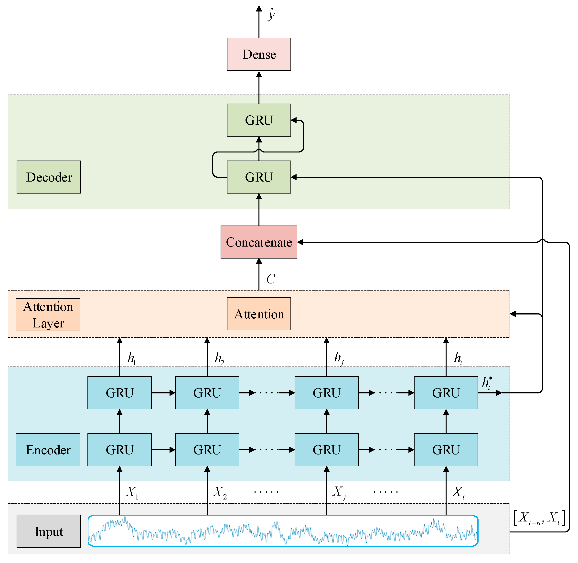
2.3. Attention-Based Codec Prediction Model
2.4. Bayesian Optimization for Global Hyperparameters
3. Results
3.1. Datasets and Setup
3.2. Evaluation Metrics
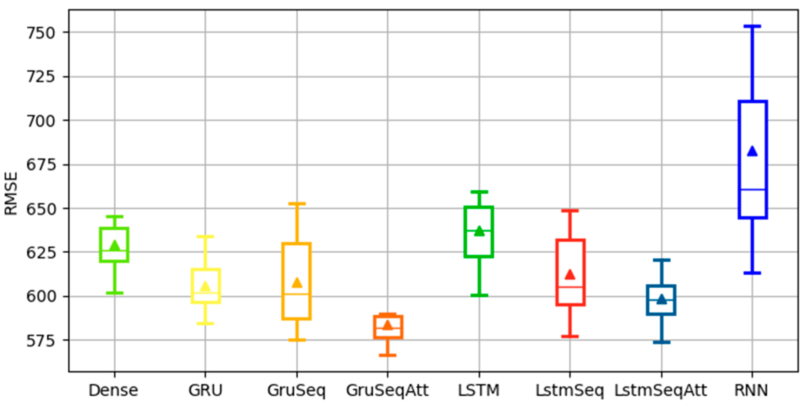
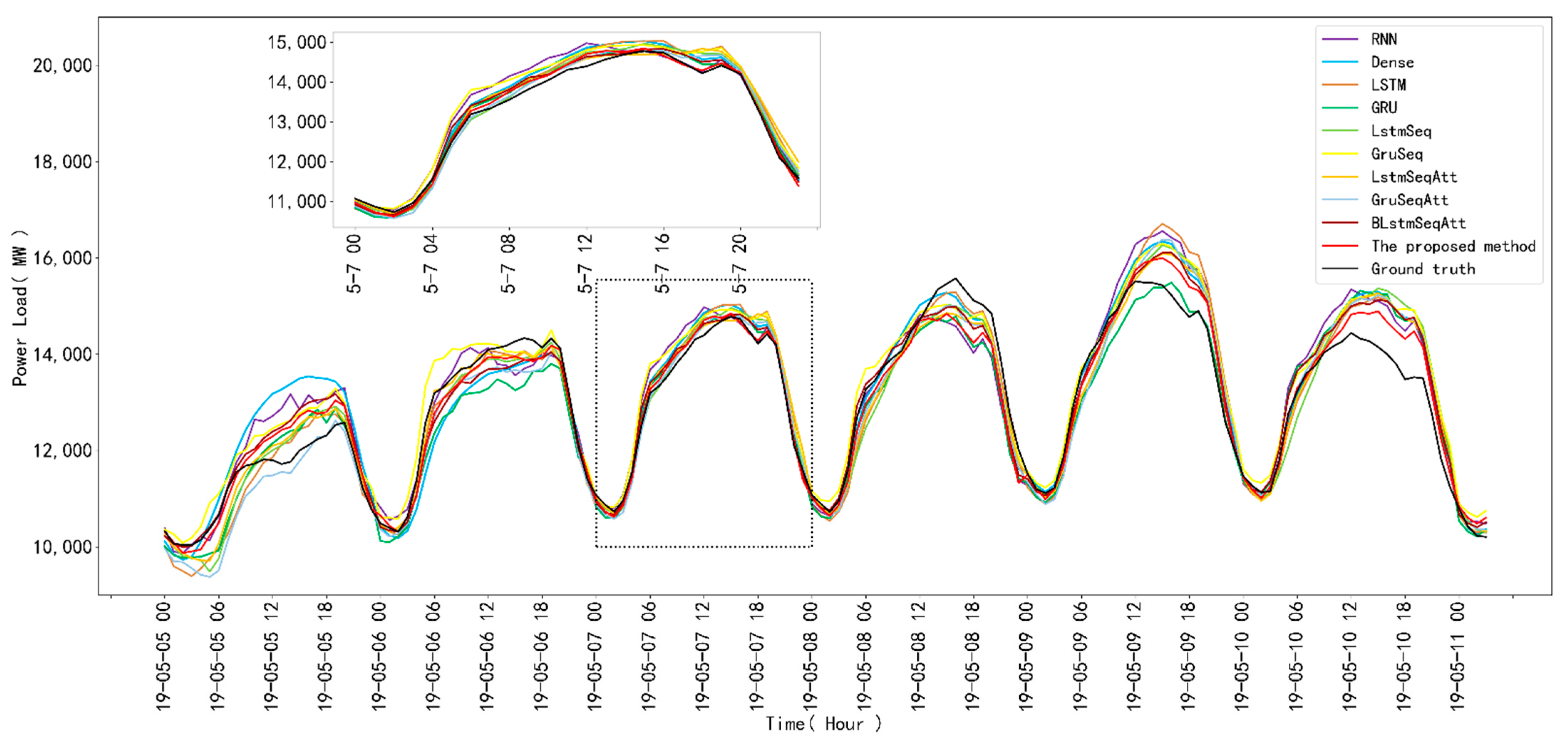
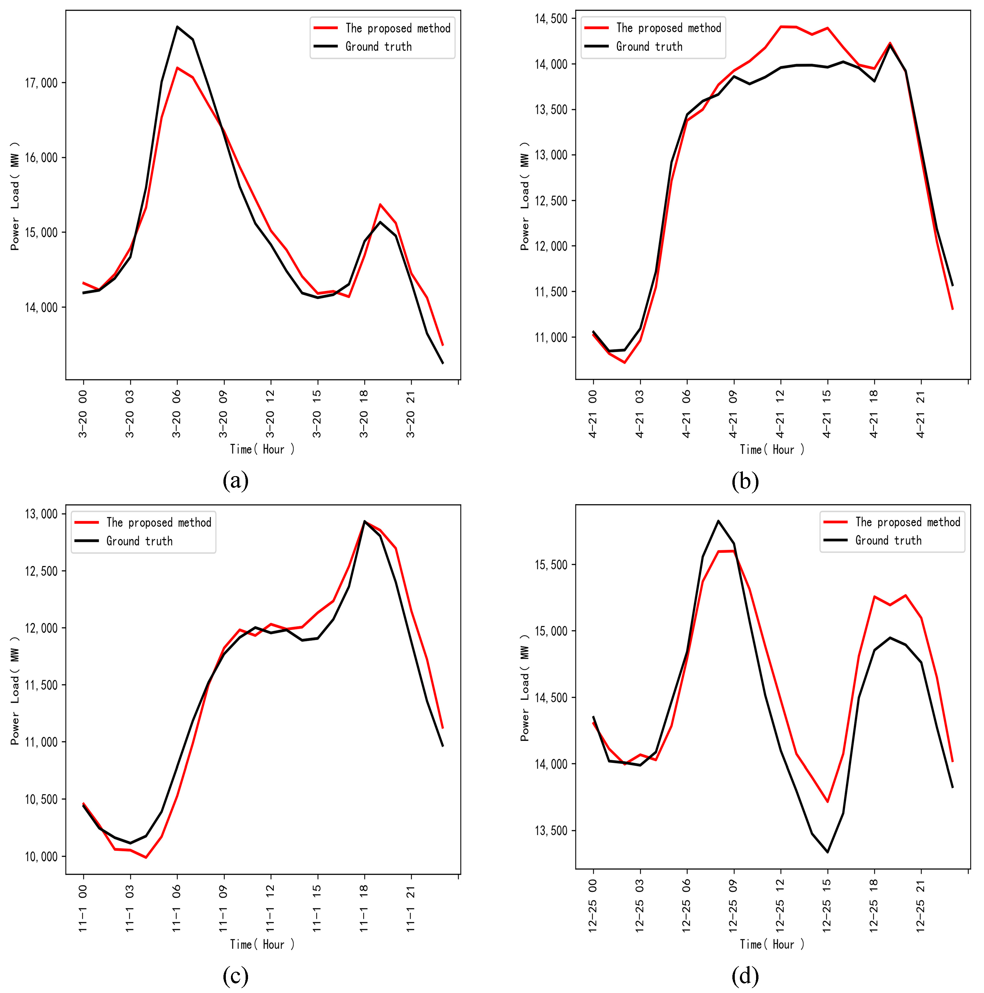
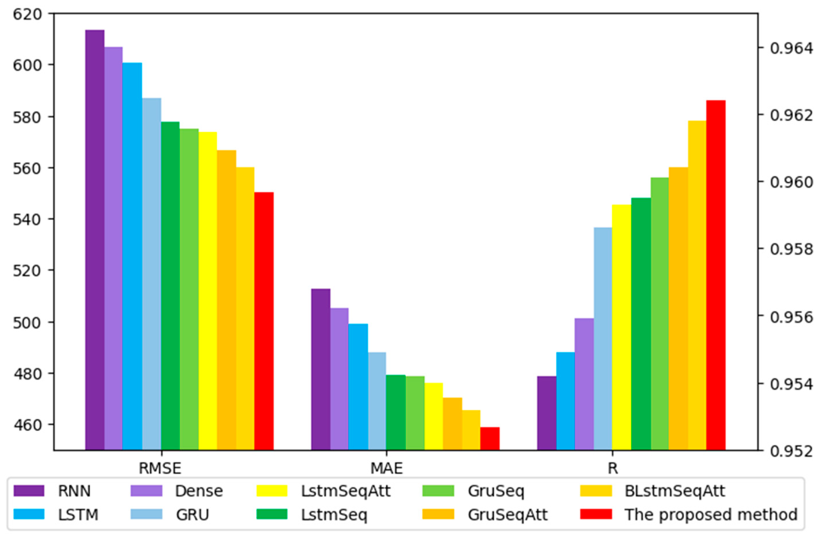
3.3. Comparative Prediction Results
4. Conclusions
Author Contributions
Funding
Institutional Review Board Statement
Informed Consent Statement
Data Availability Statement
Conflicts of Interest
References
- Jin, X.B.; Wang, H.X.; Wang, X.Y.; Bai, Y.T.; Su, T.L.; Kong, J.L. Deep-Learning Prediction Model with Serial Two-Level De-composition Based on Bayesian Optimization. Complexity 2020, 1–14. [Google Scholar] [CrossRef]
- Ge, W.; Wang, S.; Zhang, Z.; Yang, K.; Su, A. The Method of High Speed Railway Load Ultra-Short-Term Forecast Based on Dispatching and Control Cloud Platform. In Proceedings of the International Conference on Information and Automation (ICIA), Fujian, China, 20–23 June 2018; pp. 722–727. [Google Scholar]
- Zhong, H.W.; Tan, Z.F.; He, Y.L.; Xie, L.; Kang, C.Q. Implications of COVID-19 for the electricity industry: A comprehensive review. CSEE J. Power Energy Syst. 2020, 6, 489–495. [Google Scholar] [CrossRef]
- Guo, X.; Zhao, Q.; Zheng, D.; Ning, Y.; Gao, Y. A short-term load forecasting model of multi-scale cnn-lstm hybrid neural network considering the real-time electricity price. Energy Rep. 2020, 6, 1046–1053. [Google Scholar] [CrossRef]
- Haq, E.U.; Lyu, X.; Jia, Y.; Hua, M.; Ahmad, F. Forecasting household electric appliances consumption and peak demand based on hybrid machine learning approach. Energy Rep. 2020, 6, 1099–1105. [Google Scholar] [CrossRef]
- Pang, Y.; He, Y.; Jiao, J.; Cai, H. Power load demand response potential of secondary sectors in china: The case of western inner mongolia. Energy 2020, 192, 1–11. [Google Scholar] [CrossRef]
- Fumo, N.; Rafe Biswas, M.A. Regression analysis for prediction of residential energy consumption. Renew. Sustain. Energy Rev. 2015, 47, 332–343. [Google Scholar] [CrossRef]
- Yi, S.L.; Jin, X.B.; Su, T.L.; Tang, Z.Y.; Wang, F.F.; Xiang, N.; Kong, J.L. Online Denoising Based on the Second-Order Adaptive Statistics Model. Sensors 2017, 17, 1668–1685. [Google Scholar] [CrossRef] [PubMed] [Green Version]
- Liu, Z.; Wang, X.; Zhang, Q.; Huang, C. Empirical mode decomposition based hybrid ensemble model for electrical energy consumption forecasting of the cement grinding process. Measurement 2019, 138, 314–324. [Google Scholar] [CrossRef]
- Holt, C.C. Forecasting seasonals and trends by exponentially weighted moving averages. Int. J. Forecast. 2004, 20, 5–10. [Google Scholar] [CrossRef]
- Fan, C.L.; Ding, Y.F.; Liao, Y.D. Analysis of hourly cooling load prediction accuracy with data-mining approaches on different training time scales-ScienceDirect. Sustain. Cities Soc. 2019, 51, 101717. [Google Scholar] [CrossRef]
- Liao, Z.; Gai, N.; Stansby, P.; Li, G. Linear non-causal optimal control of an attenuator type wave energy converter m4. IEEE Trans. Sustain. Energy 2019, 99, 1. [Google Scholar] [CrossRef] [Green Version]
- Khashei, M.; Bijari, M. A novel hybridization of artificial neural networks and arima models for time series forecasting. Appl. Soft Comput. 2011, 11, 2664–2675. [Google Scholar] [CrossRef]
- Jin, X.B.; Yang, N.X.; Wang, X.Y.; Bai, Y.T.; Kong, J.L. Hybrid deep learning predictor for smart agriculture sensing based on empirical mode decomposition and gated recurrent unit group model. Sensors 2020, 20, 1334. [Google Scholar] [CrossRef] [PubMed] [Green Version]
- Yang, A.Q.; Yu, X.H.; Su, T.L.; Jin, X.B.; Kong, J.L. Broad learning system for human activity recognition using sensor data. Int. J. Comput. Appl. Technol. 2019, 61, 259. [Google Scholar] [CrossRef]
- Bian, H.; Zhong, Y.; Sun, J.; Shi, F. Study on power consumption load forecast based on k-means clustering and fcm–bp model. Energy Rep. 2020, 6, 693–700. [Google Scholar] [CrossRef]
- Liu, T.; Tan, Z.; Xu, C.; Chen, H.; Li, Z. Study on deep reinforcement learning techniques for building energy consumption forecasting. Energy Build. 2020, 208, 109675.1–109675.14. [Google Scholar] [CrossRef]
- Fu, Y.; Li, Z.; Zhang, H.; Xu, P. Using support vector machine to predict next day electricity load of public buildings with sub-metering devices. Procedia Eng. 2015, 121, 1016–1022. [Google Scholar] [CrossRef] [Green Version]
- Santos, P.J.; Martins, A.G.; Pires, A.J. Designing the input vector to ann-based models for short-term load forecast in electricity distribution systems. Int. J. Electr. Power Energy Syst. 2007, 29, 338–347. [Google Scholar] [CrossRef] [Green Version]
- Fan, G.F.; Peng, L.L.; Hong, W.C.; Sun, F. Electric load forecasting by the svr model with differential empirical mode decomposition and auto regression. Neurocomputing 2016, 173, 958–970. [Google Scholar] [CrossRef]
- Pal, S.S.; Kar, S. A hybridized forecasting method based on weight adjustment of neural network using generalized type-2 fuzzy set. Int. J. Fuzzy Syst. 2019, 21, 308–320. [Google Scholar] [CrossRef]
- Wang, Y.; Niu, D.; Ji, L. Short-term power load forecasting based on ivl-bp neural network technology. Syst. Eng. Procedia 2012, 4, 168–174. [Google Scholar] [CrossRef] [Green Version]
- Jin, Y.; Wang, B.; Kong, J. Deep hybrid model based on emd with classification by frequency characteristics for long-term air quality prediction. Mathmatics 2020, 1, 214. [Google Scholar] [CrossRef] [Green Version]
- Shi, Z.G.; Bai, Y.T.; Jin, X.B.; Wang, X.Y.; Su, T.L.; Kong, J.L. Parallel deep prediction with covariance intersection fusion on non-stationary time series. Knowl. Based Syst. 2020, 211, 106523. [Google Scholar] [CrossRef]
- Zheng, Y.Y.; Kong, J.L.; Jin, X.B.; Wang, X.Y.; Su, T.L. CropDeep: The Crop Vision Dataset for Deep-Learning-Based Classification and Detection in Precision Agriculture. Sensors 2019, 19, 1058. [Google Scholar] [CrossRef] [Green Version]
- Peng, S.Y.; Su, T.L.; Jin, X.B.; Kong, J.L.; Bai, Y.T. Pedestrian motion recognition via conv-vlad integrated spatial-temporal-relational network. IET Intell. Transp. Syst. 2020, 14, 392–400. [Google Scholar] [CrossRef]
- Jin, X.B.; Lian, X.F.; Su, T.L.; Miao, B.B. Closed-Loop Estimation for Randomly Sampled Measurements in Target Tracking System. Math. Probl. Eng. 2014, 2014, 1–12. [Google Scholar] [CrossRef] [Green Version]
- Li, Z.M.; Bao, S.Q.; Gao, Z.L. Short term prediction of photovoltaic power based on fcm and cg-dbn combination. J. Electr. Eng. Technol. 2019, 15, 1–9. [Google Scholar] [CrossRef]
- Son, N.; Yang, S.; Na, J. Deep neural network and long short-term memory for electric power load forecasting. Appl. Sci. 2020, 10, 6489. [Google Scholar] [CrossRef]
- Kang, T.; Lim, D.Y.; Tayara, H.; Chong, K.T. Forecasting of power demands using deep learning. Appl. Sci. 2020, 10, 7241. [Google Scholar] [CrossRef]
- Jin, X.B.; Yu, X.H.; Su, T.L.; Yang, D.N.; Wang, L. Distributed deep fusion predictor for amulti-sensor system based on causality entropy. Entropy 2021, 23, 219. [Google Scholar] [CrossRef]
- Jin, X.; Yang, N.; Wang, X.; Bai, Y.; Kong, J. Integrated predictor based on decomposition mechanism for pm2.5 long-term prediction. Appl. Sci. 2019, 9, 4533. [Google Scholar] [CrossRef] [Green Version]
- Rahman, A.; Srikumar, V.; Smith, D. Predicting electricity consumption for commercial and residential buildings using deep recurrent neural networks. Appl. Energy 2018, 212, 372–385. [Google Scholar] [CrossRef]
- Alzahrani, A.; Shamsi, P.; Ferdowsi, M.; Dagli, C. Solar irradiance forecasting using deep recurrent neural networks. In Proceedings of the 6th International Conference on Renewable Energy Research and Applications (ICRERA), San Diego, CA, USA, 5–8 November 2017; pp. 988–994. [Google Scholar]
- Mohamed, M. Parsimonious memory unit for recurrent neural networks with application to natural language processing. Neurocomputing 2018, 314, 48–64. [Google Scholar] [CrossRef]
- Hochreiter, S.; Schmidhuber, J. Long short-term memory. Neural Comput. 1997, 9, 1735–1780. [Google Scholar] [CrossRef] [PubMed]
- Bouktif, S.; Fiaz, A.; Ouni, A.; Serhani, M.A. Optimal deep learning lstm model for electric load forecasting using feature selection and genetic algorithm: Comparison with machine learning approaches. Energies 2018, 11, 1636. [Google Scholar] [CrossRef] [Green Version]
- Wang, Y.; Gan, D.; Sun, M.; Zhang, N.; Zongxiang, L. Probabilistic individual load forecasting using pinball loss guided lstm. Appl. Energy 2019, 235, 10–20. [Google Scholar] [CrossRef] [Green Version]
- Toubeau, J.F.; Bottieau, J.; Vallee, F.; Greve, Z.D. Deep learning-based multivariate probabilistic forecasting for short-term scheduling in power markets. IEEE Trans. Power Syst. 2019, 34, 1203–1215. [Google Scholar] [CrossRef]
- Wang, Y.; Liao, W.; Chang, Y. Gated recurrent unit network-based short-term photovoltaic forecasting. Energies 2018, 11, 2163. [Google Scholar] [CrossRef] [Green Version]
- Afrasiabi, M.; Mohammadi, M.; Rastegar, M.; Stankovic, L.; Khazaei, M. Deep-based conditional probability density function forecasting of residential loads. IEEE Trans. Smart Grid 2020, 11, 3646–3657. [Google Scholar] [CrossRef] [Green Version]
- Sutskever, I.; Vinyals, O.; Le, Q.V. Sequence to sequence learning with neural networks. Adv. Neural Inf. Process. Syst. 2014, 2, 3104–3112. [Google Scholar]
- Malhotra, P.; Ramakrishnan, A.; Anand, G.; Vig, L.; Shroff, G. Lstm-based encoder-decoder for multi-sensor anomaly detection. arXiv 2016, arXiv:1607.00148. [Google Scholar]
- Qin, Y.; Song, D.; Chen, H.; Cheng, W.; Jiang, G.; Cottrell, G. A dual-stage attention-based recurrent neural network for time series prediction. In Proceedings of the Twenty-Sixth International Joint Conference on Artificial Intelligence, IJCAI, Melbourne, Australia, 19–25 August 2017; pp. 2627–2633. [Google Scholar] [CrossRef] [Green Version]
- Bottieau, J.; Hubert, L.; Greve, Z.D.; François, V.; François, J.T. Very-short-term probabilistic forecasting for a risk-aware participation in the single price imbalance settlement. IEEE Trans. Power Syst. 2019, 35, 1218–1230. [Google Scholar] [CrossRef]
- Mashlakov, A.; Tikka, V.; Lensu, L.; Romanenko, A.; Honkapuro, S. Hyper-Parameter Optimization of Multi-Attention Recurrent Neural Network for Battery State-of-Charge Forecasting. In Proceedings of the Progress in Artificial Intelligence, Vila Real, Portugal, 3–6 September 2019; pp. 482–494. [Google Scholar]
- Sehovac, L.; Nesen, C.; Grolinger, K. Forecasting Building Energy Consumption with Deep Learning: A Sequence to Sequence Approach. In Proceedings of the International Congress on Internet of Things, Milan, Italy, 8–13 July 2019; pp. 108–116. [Google Scholar]
- Du, S.; Li, T.; Yang, Y.; Horng, S.J. Multivariate time series forecasting via attention-based encoder-decoder framework. Neurocomputing 2020, 12, 388. [Google Scholar] [CrossRef]
- Snoek, J.; Larochelle, H.; Adams, R.P. Practical bayesian optimization of machine learning algorithms. In Proceedings of the 25th International Conference on Neural Information Processing Systems, Granada, Spain, 20 November 2020; Volume 2, pp. 2951–2959. [Google Scholar]
- Tang, R.; Zeng, F.; Chen, Z.; Wang, J.S.; Wu, Z. The comparison of predicting storm-time ionospheric tec by three methods: Arima, lstm, and seq2seq. Atmosphere 2020, 11, 316. [Google Scholar] [CrossRef] [Green Version]
- Bahdanau, D.; Cho, K.; Bengio, Y. Neural machine translation by jointly learning to align and translate. Computer ence. arXiv 2014, arXiv:1409.0473. [Google Scholar]
- Luong, M.; Pham, H.; Manning, C.D. Effective approaches to attention-based neural machine translation. arXiv 2015, arXiv:1508.04025. [Google Scholar]
- Shahriari, B.; Swersky, K.; Wang, Z.; Adams, R.P.; De, F. Taking the human out of the loop: A review of Bayesian optimization. Proc. IEEE 2015, 104, 148–175. [Google Scholar] [CrossRef] [Green Version]
- Abbasimehr, H.; Paki, R. Prediction of COVID-19 confirmed cases combining deep learning methods and Bayesian optimization. Chaos Solitons Fractals 2021, 142, 110511. [Google Scholar] [CrossRef]
- Zhang, K.; Zheng, L.; Liu, Z.; Ning, J. A deep learning based multitask model for network-wide traffic speed prediction. Neurocomputing 2019, 10, 97–101. [Google Scholar] [CrossRef]
- Shakibjoo, A.D.; Moradzadeh, M.; Moussavi, S.Z.; Vandevelde, L. A novel technique for load frequency control of multi-area power systems. Energies 2020, 13, 2125. [Google Scholar] [CrossRef]
- Zhang, J.S.; Xiao, X.C. Predicting chaotic time series using recurrent neural network. Chin. Phys. Lett. 2008, 17, 88. [Google Scholar] [CrossRef]
- Gers, F.A.; Schraudolph, N.N. Learning precise timing with lstm recurrent networks. J. Mach. Learn. Res. 2003, 3, 115–143. [Google Scholar] [CrossRef]
- Li, H.; Liu, H.; Ji, H.; Zhang, S.; Li, P. Ultra-short-term load demand forecast model framework based on deep learning. Energies 2020, 13, 4900. [Google Scholar] [CrossRef]
- Habler, E.; Shabtai, A. Using LSTM encoder-decoder algorithm for detecting anomalous ADS-B messages. Comput. Secur. 2018, 78, 155–173. [Google Scholar] [CrossRef] [Green Version]


| Hyperparameter | Data Type | Values Range | PL | PG |
|---|---|---|---|---|
| Attention layer similarity matrix dimensions | integer | {1} + {2–64} step 2 | 18 | 4 |
| Encoder network layers | integer | {1–6} step 1 | 2 | 6 |
| Decoder network layers | integer | {1–6} step 1 | 5 | 2 |
| Number of encoder network units | integer | {8–128} step 8 | 120 | 72 |
| Number of decoder network units | integer | {8–128} step 8 | 120 | 72 |
| Number of data inputing decoder | integer | {0–24} step 1 | 6 | 23 |
| Batch size of training data | integer | {1} + {2–64} step 2 | 8 | 10 |
| Number of training epochs | integer | {60–200} step 5 | 130 | 155 |
| Model training optimizer | categorical | {Adam, Nadam, SGD} | Adam | Adam |
| Model | RMSE | MAE | R | SMAPE | NRMSE |
|---|---|---|---|---|---|
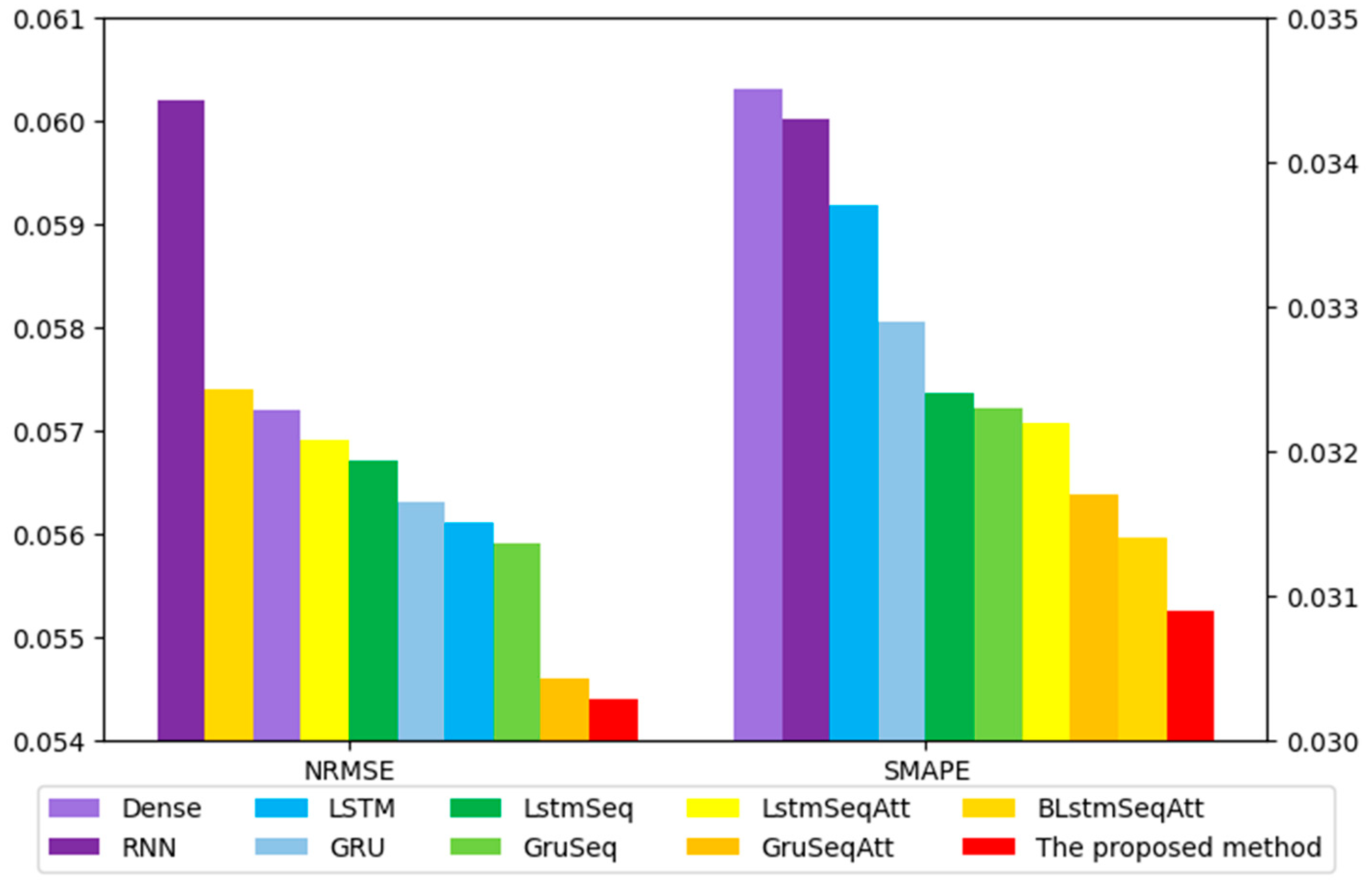
| Dense [56] | 606.7183 | 504.9654 | 0.9559 | 0.0343 | 0.0602 |
| RNN [57] | 613.2839 | 512.6149 | 0.9542 | 0.0345 | 0.0572 |
| LSTM [58] | 600.4019 | 498.8333 | 0.9549 | 0.0337 | 0.0561 |
| GRU [59] | 586.8837 | 487.9156 | 0.9586 | 0.0329 | 0.0563 |
| LstmSeq [60] | 577.462 | 479.0576 | 0.9595 | 0.0324 | 0.0567 |
| GruSeq | 575.1462 | 478.5666 | 0.9601 | 0.0323 | 0.0559 |
| LstmSeqAtt | 573.7516 | 475.9956 | 0.9593 | 0.0322 | 0.0569 |
| GruSeqAtt | 566.5466 | 470.2515 | 0.9604 | 0.0317 | 0.0546 |
| BLstmSeqAtt | 560.0931 | 465.4894 | 0.9618 | 0.0314 | 0.0574 |
| Proposed method | 550.3955 | 458.9382 | 0.9624 | 0.0309 | 0.0544 |
Publisher’s Note: MDPI stays neutral with regard to jurisdictional claims in published maps and institutional affiliations. |
© 2021 by the authors. Licensee MDPI, Basel, Switzerland. This article is an open access article distributed under the terms and conditions of the Creative Commons Attribution (CC BY) license (http://creativecommons.org/licenses/by/4.0/).
Share and Cite
Jin, X.-B.; Zheng, W.-Z.; Kong, J.-L.; Wang, X.-Y.; Bai, Y.-T.; Su, T.-L.; Lin, S. Deep-Learning Forecasting Method for Electric Power Load via Attention-Based Encoder-Decoder with Bayesian Optimization. Energies 2021, 14, 1596. https://doi.org/10.3390/en14061596
Jin X-B, Zheng W-Z, Kong J-L, Wang X-Y, Bai Y-T, Su T-L, Lin S. Deep-Learning Forecasting Method for Electric Power Load via Attention-Based Encoder-Decoder with Bayesian Optimization. Energies. 2021; 14(6):1596. https://doi.org/10.3390/en14061596
Chicago/Turabian StyleJin, Xue-Bo, Wei-Zhen Zheng, Jian-Lei Kong, Xiao-Yi Wang, Yu-Ting Bai, Ting-Li Su, and Seng Lin. 2021. "Deep-Learning Forecasting Method for Electric Power Load via Attention-Based Encoder-Decoder with Bayesian Optimization" Energies 14, no. 6: 1596. https://doi.org/10.3390/en14061596