
An Ensemble Energy Consumption Forecasting Model Based on Spatial-Temporal Clustering Analysis in Residential Buildings


1
Department of Computer Engineering, Jeju National University, Jejusi 63243, Korea
2
Department of Computer Science, Attock Campus, COMSATS University Islamabad, Attock 43600, Pakistan
*
Author to whom correspondence should be addressed.
Energies 2021, 14(11), 3020; https://doi.org/10.3390/en14113020
Submission received: 25 March 2021
/
Revised: 12 May 2021
/
Accepted: 18 May 2021
/
Published: 23 May 2021
(This article belongs to the Special Issue Machine Learning-Based Energy Forecasting and Its Applications)
Abstract
:Due to the availability of smart metering infrastructure, high-resolution electric consumption data is readily available to study the dynamics of residential electric consumption at finely resolved spatial and temporal scales. Analyzing the electric consumption data enables the policymakers and building owners to understand consumer’s demand-consumption behaviors. Furthermore, analysis and accurate forecasting of electric consumption are substantial for consumer involvement in time-of-use tariffs, critical peak pricing, and consumer-specific demand response initiatives. Alongside its vast economic and sustainability implications, such as energy wastage and decarbonization of the energy sector, accurate consumption forecasting facilitates power system planning and stable grid operations. Energy consumption forecasting is an active research area; despite the abundance of devised models, electric consumption forecasting in residential buildings remains challenging due to high occupant energy use behavior variability. Hence the search for an appropriate model for accurate electric consumption forecasting is ever continuing. To this aim, this paper presents a spatial and temporal ensemble forecasting model for short-term electric consumption forecasting. The proposed work involves exploring electric consumption profiles at the apartment level through cluster analysis based on the k-means algorithm. The ensemble forecasting model consists of two deep learning models; Long Short-Term Memory Unit (LSTM) and Gated Recurrent Unit (GRU). First, the apartment-level historical electric consumption data is clustered. Later the clusters are aggregated based on consumption profiles of consumers. At the building and floor level, the ensemble models are trained using aggregated electric consumption data. The proposed ensemble model forecasts the electric consumption at three spatial scales apartment, building, and floor level for hourly, daily, and weekly forecasting horizon. Furthermore, the impact of spatial-temporal granularity and cluster analysis on the prediction accuracy is analyzed. The dataset used in this study comprises high-resolution electric consumption data acquired through smart meters recorded on an hourly basis over the period of one year. The consumption data belongs to four multifamily residential buildings situated in an urban area of South Korea. To prove the effectiveness of our proposed forecasting model, we compared our model with widely known machine learning models and deep learning variants. The results achieved by our proposed ensemble scheme verify that model has learned the sequential behavior of electric consumption by producing superior performance with the lowest MAPE of 4.182 and 4.54 at building and floor level prediction, respectively. The experimental findings suggest that the model has efficiently captured the dynamic electric consumption characteristics to exploit ensemble model diversities and achieved lower forecasting error. The proposed ensemble forecasting scheme is well suited for predictive modeling and short-term load forecasting.
1. Introduction
The energy consumed by residential buildings has dramatically increased over the past few years due to technological advancements, rapid urbanization, occupant indoor stay time and comfort index, etc. [1]. According to International Energy Agency (IEA) the residential buildings consume about 40% of the energy consumption in the US and EU [2]. To overcome these problems, an accurate electric consumption forecast can help achieve energy efficiency, reduce electricity wastage, and mitigate global climate changes [3]. Besides limiting the chances of over and underproduction of electricity, accurate consumption forecasts can help understand the spatial and temporal variations of building electric consumption, delivering responsive demand-side management [4]. Analysis of consumption profiles of various users enables more profound insights into electric consumption patterns observed 24-h a day so that policymakers can devise appropriate strategies for achieving demand flexibility [5]. Furthermore, target specific consumer groups based on consumption profiles (low, average, high) for reducing electric consumption during peak consumption hours and prompt them towards time-sensitive use of electricity [5].
The system urban computing architectures are becoming increasingly popular for data analysis generated by devices such as smart meters installed in residential buildings to improve quality of life. Advances in technology, computing power, Artificial Intelligence (AI), and Machine Learning (ML) have paved the way for addressing many urban computing problems like short-term electric consumption forecasting. This has been possible because of cutting-edge research technologies and breakthroughs in data acquisition, analytics, data transmission rate exponential growth of storage capacity and processing power. Researchers are now more empowered to handle big data and utilize it more efficiently for improving life quality.
In recent times, sustainable energy generation systems are distinguished by achieving energy-efficient systems, net-zero energy buildings, implementing effective energy management strategies, generating electricity using non-renewable energy resources, electricity flow, and information using integrated communication technologies, signal processing, and control [6]. All such activities require management of electric production and consumption based on communication networks that facilitate data acquisition and control so that we can implement green energy management strategies effectively [7]. Green and NetZero energy buildings based on green communication technologies are the most substantial part of sustainable urban power systems [8]. The prime focus of these systems revolve around energy-efficient buildings. Building energy management (BEM) and Apartment Energy Management (AEM) are two challenging research areas because of the uncertainty in electric consumption and demand-side management influenced by various factors such as occupant behavior, intrinsic work routines, schedule of operations, comfort index and outdoor weather conditions [9,10,11].
Furthermore, the addition of renewables such as solar and wind-based energy generation systems, rechargeable electric gadgets, and vehicles introduce random and uncertainty to occupant electric consumption patterns [12]. A solution for accurate electric consumption in coordination with green communication technologies at apartment level, floor level, and building level is highly desirable at the present moment so that energy efficiency can be achieved, resource wastage can be avoided, and policymakers can make macro-decisions for introducing economic regulations. Accurately forecasted electric consumption in case of deregulated electricity market assists the building energy managers to sell the excessive electricity through efficient scheduling with better control of energy resources and electric consumption. Lower forecasting accuracy and uncertain electricity consumption could lead to inefficient energy management, wastage of scarce non-renewable resources, and incurred additional costs.
Recently smart metering infrastructure has provided access to high-resolution electric consumption data that has enabled researchers to analyze consumers’ load profiles using cluster analysis. Electric consumption profiles are a crucial element of energy system models. They depict the fluctuations and variations in consumption and describe the relative demand-supply of electricity for particular consumer groupings [13]. Grouping similar consumption patterns into one group based on cluster analysis is an algorithmic approach for identifying homogeneity of consumption data provided no apriori grouping existed previously. Cluster analysis has many practical applications; for instance, cluster analysis can be used to find hidden characteristics of data that strongly correlate to the consumption patterns of electricity, resultantly more appropriate and consumer-centric tariffs can be formulated accordingly.
Moreover, following this approach, high consumption consumers could be targeted for special demand response programs. Additionally, electric utilities can identify specific consumer groups to target opportunities leading to potential energy savings so that demand-side energy resource management could be effectively coordinated. Electric consumption varies in terms of building, type of load, energy use behaviors, operating times, etc. That’s why electric consumption in industrial and commercial buildings show similar patterns across the day, possessing stationary sequences and lesser variations within fixed schedules of operations [14]. However, variability in the residential context makes electric consumption forecasting a challenging task that requires specialized model development considering spatial and temporal scales.
Electric consumption forecasting during the past decade has become an established research field due to its enormous impacts on energy efficiency and sustainable power generation systems. The literature on electric consumption forecasting is growing day by day. The researchers are harnessing the power of advanced data analytics, AI, and ML to develop efficient and more generalized consumption forecasting models. Previously developed Short-term Load Forecasting (STLF) models are based on statistical approaches such as support vector Regression (SVR), smoothing techniques like Auto-regressive Moving Average (ARMA), an Auto-regressive Integrated Moving Average (ARIMA) [15]. Statistical methods require a large dataset for training; moreover, they involve colinear variables, i.e., the correlation between potential predictor variables in regression models causes difficulty in predicting dependent variables that affect the model’s statistical significance. Hence conventional models are not suitable for capturing complex electric consumption patterns and can only achieve satisfactory performance when tackling linear problems [16].
Additionally, they are unable to handle concept drift and noisy behavior of electric consumption patterns. These days, researchers are investing more resources in improving the forecasting accuracy by employing complex and highly variable electric consumption patterns through the use of advanced ML techniques [17]. The following ML methods, including Artificial Neural Networks (ANN) and Support vector Machines (SVM), are extensively utilized by researchers for electric consumption forecasting. However, conventional ML methods are prone to get stuck in local minima because of the inefficient configuration of parameters setting. For instance, in the case of ANN, they possess inherent complexity, lack of generalization ability leading to overfitting issues. To overcome limitations found in existing systems, we require an ensemble prediction model that harnesses the hidden potential of Deep Learning (DL) models as ensembles. Ensemble models deliver excellent performance as they can overcome the limitations of individual models.
Our proposed work have the following notable research contributions.
- We presented a spatial and temporal ensemble forecasting scheme involving cluster analysis for short term energy consumption forecasting.
- An ensemble electric energy forecasting model is developed based on LSTM and GRU using the stacking technique to forecast daily, weekly, and monthly energy consumption at three spatial scales; building, floor and apartment levels.
- Through cluster preprocessing at apartment level we presented consumer segmentation based on electric consumption profiles. Moreover we discovered how the cluster analysis impacts the model performance compared to without clustering.
- Based on clustering we established a classification of consumers and analyzed the temporal variations in electric consumption patterns to produce more forecastable consumer groupings.
- Furthermore we analyzed the impact of spatial-temporal granularity on model predictive performance.
We developed a robust predictive ensemble model based on stacking to provide better generalization to data and adaption to unseen and varying scenarios without getting stuck in local optimum solutions. Our proposed spatial and temporal ensemble forecasting model integrates an unsupervised k-mean clustering approach with a supervised learning approach to produce accurate consumption forecasts at the apartment level. We trained separate models to forecast electric consumption based on aggregated consumption data at the floor and building level. LSTM is trained using data clusters generated by the k-means algorithm for apartment level. The floor and building-level aggregated consumption data are used for model training. The ensemble framework comprise of LSTM acting as a base model (first level learner). The consumption forecasts produced by the base learner are fused by the second level learner that is GRU, to enhance the forecasting accuracy. While it is critical to choose the appropriate network structure to provide various levels of abstractions by capturing nonlinear relations between input and the target variable. We opted for a deep learning model LSTM as a first-level learner and GRU as a second-level learner to provide improved learn-ability and better generalization. Moreover, we build separate models at various spatial scales, like apartment level, floor level, and building level. We produced electric consumption forecasting at three significant temporal scales including hourly, daily and weekly forecasting horizon. All the stated reasons established our choice of learners and proper network architecture selection for enhancing the accuracy of our proposed models. We trained and tested our proposed model using high-resolution electric consumption data acquired from smart meters with hourly temporal granularity. The data is collected from four residential buildings in South Korea. For evaluating the performance of the proposed model, we compared the results with state-of-the-art independent machine learning models. The results of the comparative analysis proved that our proposed ensemble prediction model achieved superior performance and can forecast the day ahead, a week ahead, and month ahead electric consumption at residential floor level, apartment (cluster level), and building level.
The rest of the paper is organized as follows. Section 2 presents the reviews the existing work on electric consumption forecasting and clustering analysis of consumption profiles. Section 3 describes the data and proposed spatial and temporal ensemble forecasting model based on clustering analysis. Section 4 presents the experimental study and validation of the proposed forecasting model. Section 5 discusses the results and experimental findings. Section 6 concludes the paper and provide future insights.
2. Related Work
This section provides a detailed review of the existing studies conducted on electric consumption forecasting relevant to our proposed work. Electric consumption forecasting is an active research area due to the availability of consumption data through smart metering infrastructure. Electric consumption data comprise complex nonlinear consumption patterns depicting seasonality, trends, and weather impacts. The highly variable electric consumption patterns in the residential context pose some serious challenges for energy modelers. These challenges include unreliable data due to (unexpected weather, malfunctioned smart meters, nonsensical or missing data) affecting the process of knowledge discovery, verification of data integrity, selection of the dynamic model, and compensating forecasting error [18]. Another challenge is the behavioral aspect of occupant behavior, resulting in various energy usage patterns. Consumption is also affected by building load type; for instance, the load of a commercial and industrial building is less variable as compared to residential contexts that occur in synchronization with the intrinsic routines of the consumer and uniformity in appliance usage based on operating hours and organized occupant activities [19]. Each of these buildings requires a different approach and input features to forecast electric consumption. In short, the electric consumption is affected by both the exogenous (tsunami, windstorms, occasional holidays, etc.) and endogenous variables, and resultingly, the actual consumption forecast differs from the forecasted one. The varied consumption patterns affect the prediction accuracy of the model.
Consequently, many solutions have been devised to deal with challenging time-series electric consumption forecasting problems based on linear and nonlinear methods. Article [20] Proposed a loss-function for comparing time series data of various lengths and dimensions based soft dynamic time warping algorithm. Linear models employ a linear function to model electric consumption by providing a strong correlation between data and utilize it to predict the next observation using the linear combination of preceding ones [21]. Nowadays, nonlinear methods based on machine learning techniques are widely used by researchers. Such methods are based on extraction of the model using historical data and then using it to predict future loads. As stated, earlier ANN-based approaches are extensively applied to this domain. In previous studies [22], the authors proposed an artificial neural network-based model to analyze how the weather predominantly affects electric consumption. Ref. [23] proposed a solution for short-term load forecasting using ANN and wavelet for micro-grids. The article [24] proposed an energy prediction model for multi-storied residential buildings using the Hidden Markov Model (HMM) and achieved better prediction accuracy compared to well-known prediction algorithms. Another study [25] builds a hybrid prediction model for short-term load forecasting based on selecting a similar day approach. Empirical Mode Decomposition (EMD) combines with a deep learning model called LSTM. Another study [26] presents an ensemble perdition model for short-term load prediction. The proposed model utilized multiple learners, such as Radial Basis Function (RBF) and extreme learning machines.
Recently [27,28] employed ANN for providing solution for short term energy consumption forecasting. Besides being widely applied, ANN has some limitations, such as no concept of memory and time, which makes it inappropriate to apply to the domain of electric consumption forecasting. ANN cannot handle long-term dependencies as exist in complex time-series consumption data, becuase electric consumption on a particular day depends on consumption on same day previous week in a given sequence. Due to the limitations of existing approaches, researchers are paying attention to exploring the novelty of other machine learning techniques to address electric consumption forecasting in residential buildings. Recently deep learning architectures are gaining popularity in energy consumption forecasting due to their proven success in various domains such as computer vision and text mining. Article [29] proposed a deep learning model to predict electric consumption. The proposed model is tested using a real dataset acquired from Spain between 2007 and 2016. Another study [30] suggested a long short term memory-based Recurrent Neural Network (RNN) for modeling energy consumption of the residential consumer. In [31] presented a short-term energy forecasting approach for a residential consumer based on LSTM. The experimental findings suggest that sequence to sequence architectures can provide various abstraction levels and handle high-resolution electric consumption data. Ensemble models provide a very efficient way to combine the strengths of various models for improving model generalizability. The authors [32] presented a stacking-based ensemble model to tackle the issue of short-term load forecasting based on the moving horizon training approach. Model weights are trained using real-time load data collected from eight buildings situated in the University of California, USA. Experimental results depict that the proposed model outperformed the single model short-term load forecasting.
LSTM was designed mainly to deal with the gradient vanishing problem in the case of RNN while tackling long-term dependencies. Moreover, LSTM has a complex architecture of hidden nodes compared to RNN, which possesses a relatively more uncomplicated structure. In [33], a novel ensemble learning approach is proposed based on LSTM and Kalman filter to predict short-term electric consumption of multi-storied residential buildings. The proposed method combined the strength of the deep learning model by using LSTM as a base learner and statistical Kalman filter as a meta-learner. Experimental findings and comparative analysis highlighted that the proposed model achieved superior performance and improved prediction accuracy than counterpart independent models. A Deep Residual Network (Res-Net) is applied to provide a solution to electric load forecasting in the article [34]. The results of the proposed model demonstrate the effectiveness of the LSTM model. A popular load forecasting approach based on a statistical method called quantile regression is proven to enhance electric load forecasting accuracy [35]. An improved version of a quantile regression model is presented in [36]. Experimental findings suggest that the proposed model show more reliable forecasting results. In [37], the authors proposed a bi-directional LSTM to forecast short-term energy consumption for enhancing peer-to-peer energy trading. In [38], the authors proved that conventional statistical models cannot handle complex load patterns and proposed a multi-learning ensemble model based on stacking to predict electric load over different horizons. SVR and ANN are employed as base learners, while Multiple Linear Regression (MLR) acted as meta-leaner. Experimental results illustrated that the proposed model surpassed the counterpart models by achieving high accuracy.
Cluster analysis works by grouping a set of objects in such a way that items in the same group (called a cluster) are more similar to each other than to those in other groups (clusters). It is a primary task of exploratory data mining. It is a common statistical data analysis technique used in many fields, including machine learning, pattern recognition, image analysis, information retrieval, and bioinformatics. Cluster analysis is not an automatic task but an iterative process of knowledge discovery or interactive multi-objective optimization that involves trial and failure. Cluster analysis has proven to be very effective for producing electric consumption forecasts. A notable study [39] proposed a clustering-based energy consumption model using k-means combined with a neural network as a forecasting model. This study [40] developed a cluster-based electric consumption prediction mechanism based on extraction of features acquired by time-series correlation based on spatial-temporal clustering analysis. The study utilizes multivariate electric consumption data to forecast future load. Article [41] clustered the load profiles based on a self-organizing map (SOM) to improve load forecasting performance. Another study [42] proposed a Dynamic Time Warping-based (DTW) solution for averaging a sequential set of data in the k-means algorithm. Furthermore, a global approach for averaging sequential sets and devising a unique strategy for average length reduction is also proposed. Load profiles have been clustered based on similarity of consumption patterns, and models are trained considering electric load dynamic characteristics. Another study employed linear regression, MLP, and support vector regression to forecast electric load. Before load forecasting, the consumers are clustered based on load using correlation-based feature extraction method [43]. Previously [44] considered various time series data representations and applied ten different forecasting methods to check their feasibility for short-term load prediction using clustering analysis for historical load data. Experimental findings suggest that the accuracy of load forecasting is significantly improved using clustering consumer profiles. Clustering analysis of load profiles combined with ensemble forecasting model is firstly developed by [45] using bootstrap aggregation and clustering; experimental results confirmed the effectiveness of the proposed method with improved consumption forecasting.
However, for multifamily and multi-storied residential buildings, electric consumption forecasting performance still needs to be improved because of high variability in residential contexts. The related work verifies the effectiveness of ensemble forecasting techniques and their ability to generalize. Furthermore, the clustering analysis if combined with the ensemble learning model would mitigate the previously existing issue. For further review on time-series energy consumption forecasting, the readers are referred to [46].
3. Proposed Ensemble Electric Consumption Forecasting Model
In this section, we describe the proposed ensemble energy consumption forecasting model based on clustering analysis. Figure 1 presents a detailed architecture of the proposed ensemble energy consumption forecasting model. Then we present the cluster analysis, and details of spatial and temporal models build to forecast the electric consumption in multi-storied residential buildings. In this work, we proposed a solution for electric consumption forecasting based on an ensemble forecasting model and clustering analysis. We acquired time-series electric consumption data acquired from smart meters installed in multifamily and multi-storied residential buildings. The historical data comprise of past 24-hourly consumption data. The proposed forecasting model’s final goal is to forecast the electric consumption at three spatial scales; apartment level, floor level, and building level. At the apartment level, we applied cluster analysis before training the forecasting model. At the building and floor level, we used the aggregated consumption data to train the ensemble model. We build models at hourly temporal forecasting scales and forecast electric consumption by learning the fitting function from historical consumption data.
To improve the forecasting accuracy, we employed a stacked ensemble model in our proposed work. Our stacked ensemble model comprises two levels. The first level learner is LSTM. In the first level, multiple individual LSTM learns and produces the output. The second level learner is GRU that is responsible for combining output from first level LSTM learners to deliver an integrated final electric consumption forecast. To develop a stacked ensemble model, we first preprocessed our data divided into three parts based on our predefined spatial scales for apartments, floors, and building levels. Figure 1 shows the architecture for our spatial and temporal ensemble forecasting model. The apartment level preprocessed electric consumption data is clustered using k-means clustering, and new data is generated based on consumption profiles of consumers; afterward, three clusters are formed based on low, medium, and high consumption. Simultaneously, floor and building-level consumption data are aggregated using average and median-based aggregation functions separately. The clustering result yields three clusters comprising maximum consumption consumer, average consumption consumer, and minimum consumption consumer. This data is supplied to the ensemble forecasting model where the first level is the LSTM learner and the second level learner is GRU. The detailed working of the proposed architecture will be described in the remaining part of this section.
3.1. Clustering Analysis of Residential Consumption Profiles
Historical consumption data consists of similar patterns frequently occurring over a certain period. Such patterns repeat, creating interdependencies among electric consumption patterns. There are inherent difficulties in transforming and presenting this data in a coherent and comprehensible format without excessive simplification [47]. Clustering analysis is a widely used approach that finds similarities in consumption profiles and groups them in one cluster. Clustering consumption profiles of consumers based on similar load patterns and grouping them helps in partitioning data set into several groups. The similarity within a group is more significant than that among groups. The selection of clustering algorithm and desired parameters like the choice of a distance metric, cluster numbers, and relative threshold for density depends on the type of dataset being used along with required results. Literature on clustering analysis reported a wide variety of clustering algorithms due to its multidisciplinary application areas such as clustering estimation, data analytics, and pattern recognition, etc. Cluster-based data analytics methods lie in two broad categories: hierarchical and partitional. The former method works by clustering the load profiles using a sequential nested partition, finally yielding a partitioned hierarchy as resulting output clusters [48]. While partitional methods group similar consumption profiles into one cluster based on objective function optimization, the sum of squared distance among clusters is minimized.
Additionally, the number of clusters in the case of partitional clustering approaches is to be predefined. There is a central part of each cluster representing the summarized descriptions of all consumption profiles of a residential consumer [49]. Thus, partitional clustering approaches are a preferable choice for complex nonlinear high-dimensional real electric consumption data sets.
3.2. Proposed K-Mean Clustering Algorithm Based on Hybrid Distance Measure
K-mean clustering is a widely employed partitional clustering method due to its ability to cluster high dimensional electric consumption datasets efficiently. The reason for choosing an unsupervised k-mean clustering approach for our proposed ensemble forecasting model has the following objectives; finding correlations between data and potential electricity consumers to be selected for specific demand and supply programs and figuring out undesired energy consumption behaviors (i.e., outliers). The proposed k-mean method based on hybrid distance calculation metrics works iteratively by grouping n consumption profiles. Each consumption profile represents hourly consumption data acquired through smart meters grouped into k clusters by minimizing the sum of squared among clusters demonstrated in Equation (1). The proposed clustering mechanism employs hybrid distance metrics for the calculation of object similarity. K-means algorithm works iteratively until convergence is achieved and stable clusters are produced.
represents the mth consumption profile , while is defined as nth center of cluster. K-mean algorithm efficiently optimize the dissimilarity with in a cluster. Using Hybrid distance metrics, the distance between the electric consumption profile and cluster centroids is computed. The purpose of using a hybrid distance metric is attributed to efficiently and objectively compute a similarity function. A distance function comprises positive values signified by a cartesian product. The enhanced hybrid distance metrics combine the effectiveness of two methods, namely Euclidean and Manhattan distance. The calculation of hybrid distance meteoric is shown in Equation (2).
The above equation merges two distance functions through average; using Manhattan distance, we can compute absolute difference between coordinate pairs while Euclidean distance finds straight line distance between two points. Afterward, we used cluster aggregation for maximum consumption, minimum consumption, and average energy consumption among all the apartments using the equation described in the architecture diagram. K-means clustering takes two input parameters; first, the number of instances to be clustered and the number of clusters to be formed. We employed hybrid distance metrics for finding the distance between input data samples and the nearest centroid. The algorithm outputs cluster centroid and cluster membership for data samples based on electric consumption profiles.The data acquired by cluster aggregation for apartment level and simple aggregation for floor and building level is used to train the ensemble forecasting model.
3.3. Cluster Aggregation
The clusters are aggregated based on minimum consumption, maximum consumption, and average consumption using the following equations. Equations (3) and (4) are used to find the maximum consumption patterns of the apartment in a specified interval of time.
where n represents the number of hours (time-interval), defines the home consumption, and represents the electricity consumption. The minimum consumption patterns of homes are calculated using Equation (5) in a given interval of time and same n and h variables are used to describe the equation. The Equation (5) describe this situation:
The average consumption is calculated by adding the consumption of all homes and dividing by number of homes so that we will get the average consumption of energy using Equation (6).
Using the aforementioned equations, we find the home having maximum, minimum, and average consumption in a given interval of time. This approach will help the customers to compare the energy consumption. Besides, the energy provider companies will find the home having maximum consumption and cluster all the users based on their consumption. Similarly, building and floor level electric consumption is aggregated using simple aggregation using mean and average. Afterward, the data is now ready to be fed to the ensemble forecasting model to train separate models for floor level, building level, and apartment level electric consumption forecasting.
3.4. Ensemble Forecasting Model
In this section, our proposed ensemble forecasting model is presented and discussed. Figure 2 presents the proposed ensemble electric consumption forecasting model based on the integration of LSTM and GRU. Motivation for selecting LSTM as a first-level learner is attributed to gating structures for controlling and regulating the flow of information and forgetting unnecessary information over time. Our ensemble forecasting model contains multiple LSTM learners due to their ability to provide better generalizations. LSTM memory block comprises of input gate, forget gate output gate having interconnected memory cells. Input gate consists of a hidden layer of sigmoid activated nodes and weighted inputs controlling activation to memory cells. The function of the output gate is to learn and filter specific activation of cells and pass the output to the next node in the network; while the forget gate decides which states to forget and which to remember, the memory cells are also reset here. LSTM stores information of recurrent networks in memory called cells. Cells control the read and write requests using analog gates. These memory cells state based on iterative guess making, propagating error back and weights adjustment through gradient descent, learns how to control data that enters leaves and get removed from the cell. The reason for choosing the GRU as a meta-learner is attributed to the limitation of the RNN regarding short-term memory. Electric consumption patterns are highly correlated; hence the learner needs to link output to previous events that occurred many time steps before, where the gradient will ultimately become too small. The weights in the case cannot be adjusted to consider those events that happened a long time ago, making the network unable to learn these long-term relationships. In long-term dependencies, the distance between the relevant information to the current point where it is needed becomes too vast. Therefore, it is challenging to learn long-term dependencies, and linking present output to remote outputs causes vanishing and exploding gradients. Exploding gradient occurs when there is an exponential growth of slope instead of decay. It is easier to solve exploding gradient as compared to vanishing gradient as they can be solved through truncated back propagation or squashed or clipped. While vanishing gradients are too small and non-workable for the network, making them harder to be solved.
The second level learner or the meta learner has a similar structure as LSTM except that GRU has a specialized gating structure of the hidden state, providing a well-defined mechanism for updating and reset the hidden state. The use of update gate and reset gate is to filter information forwarded to output. LSTM-GRU ensemble provides an improved solution to the vanishing and exploding gradient problem.
3.5. Stochastic Gradient Descent
Stochastic Gradient Descent (SGD) is successfully applied to train deep neural networks by solving slow convergence and local minima. We employed SGD firstly by shuffling the training data when the network is being trained. In step 2, the whole parameters are updated based on a small number of training data samples. With each iteration, the parameter is regularly updated towards the gradient of the loss function to reach global minima [50]. The main difference between simple gradient descent and SGD is that it chooses only a single data point instead of a whole dataset. The weights are updated using the following Equation (7).
Weights are represented as new and old weights, i and j are samples of training data at some kth iteration.
3.6. Data Acquisition and Pre-Processing
We performed extensive experimentation on high-resolution historical electric consumption data collected from four multi-storied residential buildings with 33, 33, 36, and 15 floors, respectively. The buildings are situated in Seoul, South Korea. The input features are hourly electric consumption for past k sequences, hour of the day, day of the week, day, and month. Each day records 24 hourly consumption data, so we have 24 hourly consumption readings with corresponding time-span. The dataset has consumption data corresponding to a time span of one year starting from 1 January 2010 to 31 December 2010 for floor-level, apartment level and aggregated building level. All the smart meters are connected to the sub-distribution level switch board linked with main server. The building comprises of multi-family residents having different routines and operating schedules. The data is recorded hourly with standard electric consumption measuring unit of kilowatt-hours (KWh). For supervised learning, we vary the size of training data to evaluate the impact of training size and cope with seasonal changes. The data is divided into three different training sets, i.e., (1 month long), (3 months long), and (6 months long). The testing set is a day ahead which is 24 h long. To get a detailed picture of the collected data, some basic statistics are calculated to get insight into the data distribution.
Figure 3 represents the floor level hourly electric consumption data. Electric consumption data has been plotted on y-axis while x-axis has corresponding time-stamp. The data patterns show dense and varied consumption due to variability in energy use behavior and other influencing factors like external weather conditions, occupancy and comfort levels of consumers etc.
Figure 4 present monthly analysis of entire data-set using box plot representation formerly known as five-number analysis. The energy consumption recorded in KWh is plotted along y-axis, against each month. The five entries in the box plot analysis shows the five numbers, i.e., maximum, minimum, mean, 1st quartile and 3rd quartile. The distribution of monthly electricity consumption starting form January to December shows how the electricity consumption patterns are varied across the year. It can be observed that the consumption during winter season is high, as South Korea undergoes extremely cold winters (Dec–Feb) with freezing temperatures and snowfall, therefore the use of heating systems and appliances becomes high. Thus resultant energy consumption also increases to maintain the comfort levels of occupants. Similarly, during hot and humid summers again the electric consumption becomes high to satisfy the cooling needs and maintain the indoor comfort. Likewise early summer and early winter months both show an average pattern for consumption.
Figure 5 presents daily analysis of energy consumption observed across seven days in a week. The intrinsic routines and working hours of the occupants highly influence the consumption patterns of energy. Week days show similar patterns where there is a rise in consumption during start of the day as daily activities began and this curve gradually begins to decrease during night hours and rest time. The daily consumption data also depicts some outliers that may differ because of multifamily residents staying in the building as well as unique schedule of operation may cause this energy use behaviour. Some of the outliers can clearly be seen in the distribution, which shows consumption is beyond the normal distribution boundary on some random days. Such outliers affect the generalization of the machine learning algorithm and hence lead to a higher error rate.
Figure 6 provides a season wise analysis of energy consumption using box plot analysis. Seasonality shows summer, winter, autumn and spring along with consumption of energy. The analysis show that extreme weather causes rise in consumption specially in winters and summers. While spring and autumn season observe quiet similar consumption patterns. Which clearly shows the impact of the sparse yet uniform pattern in monthly consumption. It can be analyzed from the data patterns that how the consumption distribution of electricity is varied across different months.
Time series electric consumption data is sequential, and current consumption patterns correlate with past consumption and possess temporal dependencies. Not a single observation could be considered independent of another. Therefore, original data must be preprocessed to tackle outliers, anomalies, and missing values. If outliers are not dealt with, they may be problematic, i.e., they produce lower performance results. Firstly, the historical consumption data is pre-processed by removing outliers using the three-sigma rule. It is a widely used heuristics for the detection and removal of outliers from the data. A three-sigma rule is a heuristic approach that considers all data values closer to the mean’s standard deviation. Real data is subjected to noise and non-homogeneity. For handling missing values, we employed the NAN interpolation method. Nan interpolation method efficiently replaces the importance of data that are not sampled uniformly. Due to the large span and scattering of sample data, data normalization becomes essential to ensure that weights and biases converge instability. It also helps achieve better accuracy and improvable model training. For efficient performance of sequence consumption forecasting problem, the data needs to be scaled. As LSTM is sensitive regarding scaling data, we have normalized the data with normalization of range from 0 to 1 through scaling the features so that model could converge faster and error is reduced. For normalizing data, we applied min-max scaler normalization. We scaled the time series using values from the training set to avoid information leakage from the test set. Min-Max scaler normalization works by transforming input features to a defined range. Normalization is defined as follows in Equation (8).
4. Experimental Setup
This section describes the experimental setup of the proposed research study. In this research study, Python is used as a general-purpose language to conduct a series of experiments. The well-known library sklearn is used as a core library to perform clustering and regression analysis to forecast short-term energy consumption. Furthermore, different libraries, including pandas, NumPy, Seaborn, Matplotlib, are used to process and visualize energy consumption data. Moreover, we used Microsoft Windows as an operating system (OS) along with a 3.45 GHz processor and 3.12 GB RAM to conduct experiments related to short-term energy forecasting. Table 1 briefly summarized the experimental environment of the proposed study.
5. Experimental Results and Analysis
This section presents forecasting results and cluster analysis of the proposed research study. The inputs considered for this study include hourly electric consumption, particular hour of the day, particular day of the week and week of a month. All these inputs are introduced in layer one, including 24-h electric consumption recorded for a year, for instance, 365 days × 24 h = 8760 readings. We forecasted hourly, daily, and weekly electric consumption using these inputs. However, any feature extraction has not been performed in this work. To avoid over-fitting and model biases, we employed k-fold cross-validation. To forecast weekly energy consumption, we divided our data into 52-folds of the same size. We considered the first fold as a validation Set while method fitting is done on the folds. For model testing, one-week data is used, which comprises 7 days × 24 h = 168 instances. We used the leftover data for model training, for instance, 358 days out of 365, so 365 days × 24 h = 8592 instances are utilized for model training for weekly electric consumption forecasting. Similarly, we used the past 23 h consumption data to predict the 24 hourly predictions for hourly energy consumption. For daily predictions past 168 h are used for the day ahead electric consumption of the target day. For optimal parameter setting, we employed the grid search technique. We deployed the following number of hidden neurons using the grid search approach (16, 32, 64, 128) with a learning rate starting from 0.001 to 0.01 and several epochs ranging from 50 to 200. LSTM contains six neurons and two activation functions, such as Tanh (between hidden layers) and SoftMax (between last hidden and output layers). GRU also contains a similar number of neurons providing a complimentary strength to LSTM by overcoming the limitations of individual learners. Various iterations have been tried ranging from 500 to 3000 using 100 incremental sums and 3000 set iterations based on trial and error method. The best model configuration could be selected to achieve accurate predictions.
In our proposed ensemble forecasting scheme, two approaches are implemented; clustering of electric consumption due to variations in user’s consumption behavior and ensemble model based on deep learning models. The clustering analysis aims to cluster user’s electric consumption data into three clusters, minimum consumption, maximum consumption, and average consumption. An ensemble forecasting model is proposed based on LSTM and GRU using the stacking technique to forecast the short-term electric consumption of residential buildings. Stacking is a technique used to combine several different (regression or classification) machine learning models and yield better prediction performance comparative to single models. Stacking is a stacked generalization concept that combines the results of two models for improving the overall performance of the model and avoid over-fitting. Stacking involves some initial parameters like training set, testing set, and validation set for the holdout. After applying k-fold cross-validation, the prediction results from both the training and holdout are added as new features. Hence prediction from each model adds a part of the new feature for the next-level model. The next second-level model then predicts the outcome using a test set. Basically, stacking is comprised of base learners and meta-learners; the base learner learns from the training data to make predictions and aids the meta-learner to make the final prediction by generalizing features from each layer. There are several variants of the stacking technique, but the basic one trains the base learners individually afterward they are stacked. The basic aim of stacking is to decrease the generalization error as much as possible. Furthermore, our proposed ensemble model’s forecasting results are compared with conventional deep learning models to signify the importance of the proposed work. Moreover, different statistical analysis measures are employed to evaluate the forecasting performance of the implemented deep learning models.
5.1. Cluster Analysis
The data pre-processing layer consist of finding outliers, handling missing values, sampling and normalizing the data. The sampling is carried out to reduce the data size while maintaining the original consumption patterns. For this purpose we average the data on 4 h basis for clustering at apartment level. We reduce the data to 1/4 of its original size. The sampling enhanced the processing speed without affecting the original consumption patterns. Next we have actual processing layer of the clusters and aggregations. We use aggregation for maximum consumption, minimum consumption and average consumption of the energy among all the homes. This section demonstrates our approach of clustering and visualization of high resolution electric consumption data set.For clustering we use a real data set gathered from residential buildings. The data consist of 96 apartments belonging to four residential buildings. The data is recorded for 1155 days.
Figure 7 shows the electricity consumption clusters of selected 40 homes for 1 day. The analysis shows the clustering and mean of high, medium and low consumption homes for 1 day long data. Various colors have been used to illustrate the uniqueness of each cluster, i.e., blue colors defines maximum consumption cluster, red color shows medium consumption cluster and green color shows minimum consumption cluster. The mean value representation of the the respective clusters is done using shapes. Moreover, it also depicts the maximum, average and minimum consumption utilization homes during the reported period. This results helps in finding the potential consumption patterns and misuse/wastage of energy; specially in educational building and official buildings.
Figure 8 presents the consumption clusters of 40 homes for the time-span of one week. The electric consumption for each home is plotted on y-axis against the home id on y-axis. Due the huge amount of data for each home this figure shows about 8000 records. Due to that we divide the data into samples. Moreover it also depicts the results of cluster means for minimum consumption cluster, maximum consumption cluster and average consumption cluster for the period of one day. Figure 8 presents the results of 1 week cluster analysis in the given time interval.
Figure 9 shows the cluster mean result of the electricity consumption of 40 homes in the given time interval based on minimum, average and maximum consumption cluster. The data is clustered based on the consumption in the given time interval. We defined preset consumption threshold for clustering. We divided the homes with electricity consumption into high consumption homes, average consumption homes and low consumption homes.It is evident from the cluster analysis that one home possess very high electric consumption, while three have average consumption and the rest of the homes are with low electricity consumption.
5.2. Performance Evaluation
The above hyper parameters for our proposed ensemble forecasting scheme outperformed the counterpart solutions. The data used in this study comprise of real electricity consumption data collected from four residential buildings. The data is not publicly available hence we were compelled to compare the performance of our model with the published work based on the dataset used in this study. We employed mean absolute error (MAE), mean absolute percentage error (MAPE), R2 score and root mean square error (RMSE) for performance evaluation of the proposed model [51,52]. MAPE, and RMSE are scale dependent accuracy measure.
We compared our proposed ensemble model with some benchmark machine learning and deep learning models applied to the domain of energy consumption forecasting. The comparative analysis is performed with deep learning variants namely RNN, LSTM and GRU additionally some conventional learning models including Random Forest (RF), XGBoost, AdaBoost and Gradient Boosting (GB) are part of the comparative analysis. Model testing involves the testing of prediction model using standard evaluation metrics. The proposed ensemble model outputs electric consumption forecast of target hour, day or week at apartment, floor and building level.
Figure 10 presents the performance of hourly electric consumption prediction using several independent DL variants, such as RNN, LSTM, bi-directional LSTM (Bi-LSTM) and GRU.The graphs presents the difference between actual and predicted electric consumption. It is evident from the error graph that error is quiet high in case of RNN due to long term dependencies. The low performance of RNN is seemingly low due to the fact that RNN is trained based on back propagation through time and it remembers information that occurred just a few time-steps ago, hence RNN suffers from problem of gradient vanishing/ exploding due to memory limitations. Practically, RNN have little ability to look back only a few time steps therefore it is unable to handle long term dependencies. Second error graph of Figure 10 shows the electric consumption forecasting based on LSTM, as they are proven to yield efficient performance by learning complex nonlinear electric consumption patterns. Moreover, it can provide better generalization by learning the temporal correlation that exist in electric consumption data. Third graph of Figure 10 presents the prediction performance achieved by GRU for hourly electric consumption. GRU also achieved satisfactory performance because of specialized architecture containing update and reset gates that helps model control the flow of information through specialised architectures for remembering and discarding information. Fourth error graph of Figure 10 depicts the results achieved by our proposed ensemble model. The error graph show that the actual and predicted consumption are nearly similar. The error percentage is quiet lower is case of our ensemble forecasting scheme. Experimental findings verify that the ensemble forecasting scheme attained higher precision and hence proves the effectiveness of our proposed ensemble forecasting model.
Furthermore, Figure 11 shows a comparative analysis of observed and estimated electric consumption using proposed model and Bi-LSTM. The experimental results shows that the Bi-LSTM could not perform well in case of hourly consumption forecasting. High error in case of Bi-LSTM is attributed to its consideration for future and past input data for forecasting future consumption, hence the amount of data influence the output result significantly.
Table 2 and Table 3 summarize the experimental findings of the proposed ensemble model and counterpart solutions. Firstly the experimental results of hourly electric consumption forecasting are presented at building level. The statistical analysis of the proposed ensemble model with conventional machine learning and deep learning models verify that ensemble forecasting scheme achieved the highest R2 scores and lowest error comparative to independent models. Our proposed model achieved the lowest MAPE of 4.182 and R2 score of 0.944. It is evident from statistical analysis that the proposed ensemble model performed efficiently on building level hourly electric consumption forecasting compared to the independent learners, such as RNN, LSTM, GRU, Bi-LSTM. The R2 score of the proposed ensemble model is highest among all, which verify the generalization ability and significance of the proposed model compared to the conventional deep learning models. The performance of independent LSTM learner is also competitive as it successfully achieved the second highest R2 score for hourly electric consumption prediction at building level. The low error percentage at building level is because of data aggregation and choice of stacking ensemble combining multiple sequential models that leads to improved performance. Aggregating consumption smoothens the variations in consumption patterns as compared to loads of single apartments where a higher variability and fluctuations in the load profiles are observed. As it is evident that the RNN-LSTM model predicted very well in medium to long term consumption forecasting as compared to the other counterparts which shows the strength and feasibility of the proposed RNN model for short term and medium term forecasts. The comparative results of the RNN and other established models for the forecast of daily, weekly and monthly basis. The results depicts and justify the hypothesis made in this study that sequence based model learn better generalization that the non-sequential models. The proposed RNN model outperformed other models in short term and medium term forecasts, however, Deep Extreme Learning Machines (DELM) perform better for daily consumption prediction at building level. Experimental results depict that the proposed ensemble model demonstrate superior performance compared to counterpart solutions.
Furthermore, the electric consumption forecasting results of our proposed model are evaluated and compared with baseline learning models as shown in Table 3. Performance evaluation of conventional ML models and proposed model is described in Table 3. It can be observed that the forecasting error of the proposed ensemble model is low compared to the traditional learning models for building-level hourly electric consumption models. The MAPE value of the proposed ensemble model is 4.18, which reveals that the proposed model performed efficiently compared to the baseline ML models, such as RF, XGBoost, AdaBoost, and GB. The MAPE score of conventional models including RF, XGBoost, AdaBoost, GB is 17.56, 17.82, 17.84, and 17.64, respectively.
Table 4 depicts that our proposed model produced an accurate forecast as compared to the counterpart solutions due to aggregation at floor level. The model for floor and building levels is trained using aggregated electric consumption data. At floor level, the consumption patterns of all apartments are aggregated so that energy consumption could also be predicted at floor level. As temporal variations are reduced when we aggregate the electric consumption, model forecast error is reduced. Moreover, an individual floor level model is trained and tested for each floor. Similarly, the same approach will be followed at the building level to forecast aggregated consumption of an overall building. Aggregating consumption profiles on floor level yields better results. Our proposed ensemble forecasting model achieved stable results with the lowest MAPE of 4.54 percent for the daily energy consumption forecast. In comparison, for weekly forecasts, our ensemble forecasting scheme achieved a MAPE of 4.71 percent. Thus our proposed model outperformed counterpart solutions. The core reason for the results achieved by our model is the choice of a complimentary combination of LSTM-GRU as ensembles and the ability of LSTM to learn the sequential behavior of electricity consumption on various spatial scales.
Table 5 describes the results of daily and weekly predictions at the apartment level. We performed this analysis to investigate the impact of clustering on the prediction accuracy of our model. It is evident from the experimental findings that clustering improved the generalization ability of proposed model. The comparative analysis of our proposed ensemble forecasting model with state-of-the-art machine learning models verifies the effectiveness of clustered pre-processing before model training. The ensemble forecasting model produced outstanding results by achieving the lowest MAPE score of 5.14 percent for daily prediction and 6.0 percent for weekly prediction compared to counterpart models. The high-performance score is attributed to the apartment level clustering scheme. We clustered the data at the apartment level based on the consumption profile of consumers and performed cluster aggregation based on the low, medium, and high-level consumption profiles of consumers. Our proposed model achieved improved performance with the lowest RMSE of 0.306 for daily predictions because when we apply cluster analysis, data patterns occur at multiple frequencies within the dataset. Therefore, clustering the load profiles gives additional information to the model and significantly improves the prediction accuracy of our model. However, the performance of DELM is also competitive. The forecasting horizon for apartment level clustering is day-ahead and week-ahead (daily and weekly) electric consumption forecasting. We performed a comparative analysis of the proposed ensemble model with widely used deep learning variants such as DELM, ANFIS, and ANN. Our proposed spatial and temporal electric consumption Forecasting achieved superior performance and lower error. The ensemble forecasting scheme performed efficiently, achieved far better results, and produced the lowest RMSE of 3.06 and 0.329 for daily and weekly predictions. Apartment-level consumption forecasts yield deeper insights into consumption patterns and consumer operating schedules so that consumer-wise tariffs and target demand response could be designed.
Table 6 shows daily and weekly energy forecasting accuracy in terms of MAPE, RMS, and MAE. Experimental results illustrate that our proposed model outperforms all the others solutions at the apartment level without clustering. MAPE for daily prediction is 12.76; for weekly prediction, we can see a slight rise in error with MAPE of 13.43. The performance of apartment level consumption forecasts without clustering is low compared to clustering because we did not group the apartments based on their consumption profiles. Moreover, due to diversity in human behavior, the electric consumption patterns in multistoried residential apartments are highly dissimilar; therefore, trained models might behave differently on the test set. The chance of error becomes high in this case. It can be concluded from the above table that a model that performs well in daily prediction also performs well in weekly forecasts.
5.3. Discussion
This subsection provides detailed insights of the experimental results. The main contribution of the proposed research work is to predict short-term electric consumption. Our proposed model incorporates cluster analysis as an unsupervised learning approach for clustering electric consumption at the apartment level to find out energy usage patterns to discover potential energy-saving opportunities by grouping the consumers based on the consumption into low, average, and high consumption clusters. We performed an efficient pre-processing of high-resolution electric consumption data acquired through smart meters using k-means with hybrid distance function for representation of electric consumption clusters at apartment level. At floor and building level we considered aggregated consumption for model training. The chosen hyper-parameters for proposed ensemble forecasting scheme outperformed the counterpart independent models. The comparative analysis of the proposed ensemble forecasting scheme with various machine learning models verify the effectiveness of the proposed solution. Our proposed model outperformed other prediction models for hourly, daily and weekly temporal scales by a good margin. The core reason for ensemble forecasting model to outperform is its ability to learn the sequential behavior of the electric consumption with improved generalization ability. For analysis of temporal granularity on prediction performance we aggregated the data to forecast the daily and weekly consumption. Forecasting accuracy in terms of Mean absolute percentage error for daily and weekly floor level prediction is 4.54 and 4.71 respectively. We successfully achieved higher prediction accuracy at floor level due to data aggregation. Aggregation smooths load consumption patterns related to buildings and floors hence the variations in data are reduced compared to apartment case where there is a higher variability and fluctuations in the load profiles of consumers. For building level the reported electric consumption forecasting accuracy in terms of mean absolute percentage error is 4.18.
Furthermore we presented cluster analysis to cluster load profile of consumers for capturing temporal variations in consumers electric consumption patterns. For apartment level forecasting based on clustering, our proposed model achieved far better result compared to other models with lowest RMSE of 3.06 and 0.319 for daily and weekly predictions respectively. Due to cluster analysis data pattern occur at multiple frequencies within the dataset. Hence, clustering load profiles gives an additional information to the model and significantly improves the prediction accuracy of model. However the prediction accuracy achieved by DELM is also competitive to our model. The slight rise in error is caused by the diversity in human behavior causing variability in electric consumption patterns in multi-storied residential apartments. The highly dissimilar consumption patterns causes trained model to behave differently on test data and resultant error becomes high in case. To analyze the impact of clustering on model’s predictive performance we also performed energy consumption forecasting at apartment level without clustering. The results of apartment level forecasting without clustering verified our initial proposition that clustering yields superior forecasting performance as compared to without clustering. The forecasting error in terms of MAPE at apartment level without clustering is 12.76 and 13.43 for daily and weekly predictions respectively that is the highest reported error among all. The overall results produced by our proposed model are more stable as compared to counterpart models.
Table 7 compares energy forecasting results of the proposed ensemble model with state-of-art techniques using MAPE. In [24], the authors proposed an energy forecasting model using HMM model based on multi-residential buildings data (same data as used in this work) to predict energy consumption. The MAPE value of the HMM model is 5.22, whereas our proposed ensemble model achieved a low MAPE value of 4.182. Similarly, in [53], the authors proposed an energy forecasting model based on a feed-forward back propagation neural network (FFBPNN) and achieved a MAPE value of 11.96. The comparative analysis shows that our proposed model produced a low MAPE value of 4.182 compared to the approaches presented in [24,53], respectively. Hence, our proposed ensemble model can be considered an effective solution for formulating viable policies to enhance energy management.
6. Conclusions and Future Work
Due to the increase in electricity consumption in residential and commercial buildings, the proper analysis of electricity consumption has been deemed a necessity. The electricity consumption analysis consists of electricity consumption patterns identification, the factors influencing the electricity consumption, the short-term and long-term predictions of electricity consumption, etc. Many studies exist to analyze electricity consumption in commercial buildings; however, due to the non-availability of data, the residential buildings are not very explored. Moreover, the existing energy management systems lack in the customer level energy consumption analysis and identification of potential energy consumption customers. This research study proposed a spatial and temporal ensemble electric consumption model involving clustering analysis to provide a solution for short-term electric consumption forecasting. The proposed model is based on LSTM as a first-level learner. Simultaneously, a GRU is employed in the second level learner as a meta-learner for the fusion of outputs from both learners using stacking. The algorithm selection for ensemble models has effectively complemented each other by overcoming the weaknesses when combined. LSTM-GRU are grouped to form an ensemble to improve the prediction accuracy and decrease the generalization error as much as possible.
Experimental findings and the values of statistical measures proved that our proposed spatial and temporal ensemble forecasting model surpassed the counterpart solutions and achieved superior performance compared to counterpart models. Furthermore, we analyzed the impact of spatial and temporal granularity on prediction performance. The results verified that aggregating consumption at spatial scales of building and floor yields improved prediction accuracy. Additionally, the forecasting error rises as we go farther from hourly to weekly scales. Moreover, we discovered that clustering the consumption profiles at the apartment level further decreased the forecasting error compared to without clustering. Hence we conclude that the proposed forecasting model showed promising results that can assist energy consumption management for residential buildings and urban grids. A possible future work direction is to apply this method on other large data sets to develop city-level energy consumption models and extend this work to explore more granular spatial and temporal scales to achieve better prediction accuracy.
Author Contributions
Conceptualization, A.-N.K., N.I. and D.-H.K.; Methodology, A.-N.K. and D.-H.K.; Software, A.-N.K., N.I. and A.R.; Validation, N.I., A.R., R.A. and D.-H.K.; Formal Analysis, A.-N.K., N.I. and A.R.; investigation, A.-N.K.; Data Curation, A.-N.K. and R.A.; writing—original draft preparation, A.-N.K., N.I. and A.R.; writing—review and editing, R.A. and N.I.; Visualization, N.I., A.R. and R.A.; Supervision, D.-H.K.; Project Administration, D.-H.K.; Funding Acquisition, D.-H.K. All authors have read and agreed to the published version of the manuscript.
Funding
This research was supported by Energy Cloud R&D Program through the National Research Foundation of Korea(NRF) funded by the Ministry of Science, ICT (2019M3F2A1073387), and this research was supported by Institute for Information & communications Technology Planning & Evaluation(IITP) grant funded by the Korea government(MSIT)(No.2018-0-01456, AutoMaTa: Autonomous Management framework based on artificial intelligent Technology for adaptive and disposable IoT). Any correspondence related to this paper should be addressed to Dohyeun Kim.
Institutional Review Board Statement
Not applicable.
Informed Consent Statement
Not applicable.
Data Availability Statement
Not applicable.
Conflicts of Interest
The authors declare no conflict of interest regarding the publication of this paper.
References
- Räsänen, T.; Voukantsis, D.; Niska, H.; Karatzas, K.; Kolehmainen, M. Data-based method for creating electricity use load profiles using large amount of customer-specific hourly measured electricity use data. Appl. Energy 2010, 87, 3538–3545. [Google Scholar] [CrossRef]
- Divina, F.; Gilson, A.; Goméz-Vela, F.; García Torres, M.; Torres, J.F. Stacking Ensemble Learning for Short-Term Electricity Consumption Forecasting. Energies 2018, 11, 949. [Google Scholar] [CrossRef] [Green Version]
- Lee, J.; Kim, J.; Ko, W. Day-Ahead Electric Load Forecasting for the Residential Building with a Small-Size Dataset Based on a Self-Organizing Map and a Stacking Ensemble Learning Method. Appl. Sci. 2019, 9, 1231. [Google Scholar] [CrossRef] [Green Version]
- Granell, R.; Axon, C.J.; Wallom, D.C.H. Clustering disaggregated load profiles using a Dirichlet process mixture model. Energy Convers. Manag. 2015, 92, 507–516. [Google Scholar] [CrossRef] [Green Version]
- Satre-Meloy, A.; Diakonova, M.; Grünewald, P. Cluster analysis and prediction of residential peak demand profiles using occupant activity data. Appl. Energy 2020, 260, 114246. [Google Scholar] [CrossRef]
- Ghazzai, H.; Kadri, A. Joint Demand-Side Management in Smart Grid for Green Collaborative Mobile Operators Under Dynamic Pricing and Fairness Setup. IEEE Trans. Green Commun. Netw. 2017, 1, 74–88. [Google Scholar] [CrossRef]
- Wang, K.; Li, H.; Maharjan, S.; Zhang, Y.; Guo, S. Green Energy Scheduling for Demand Side Management in the Smart Grid. IEEE Trans. Green Commun. Netw. 2018, 2, 596–611. [Google Scholar] [CrossRef]
- Collotta, M.; Pau, G. An Innovative Approach for Forecasting of Energy Requirements to Improve a Smart Home Management System Based on BLE. IEEE Trans. Green Commun. Netw. 2017, 1, 112–120. [Google Scholar] [CrossRef]
- Strasser, T.; Andrén, F.; Kathan, J.; Cecati, C.; Buccella, C.; Siano, P.; Leitão, P.; Zhabelova, G.; Vyatkin, V.; Vrba, P.; et al. A Review of Architectures and Concepts for Intelligence in Future Electric Energy Systems. IEEE Trans. Ind. Electron. 2015, 62, 2424–2438. [Google Scholar] [CrossRef] [Green Version]
- Ahmad, S.; Kim, D. Design and implementation of thermal comfort system based on tasks allocation mechanism in smart homes. Sustainability 2019, 11, 5849. [Google Scholar]
- Wahid, F.; Fayaz, M.; Aljarbouh, A.; Mir, M.; Amir, M. Energy consumption optimization and user comfort maximization in smart buildings using a hybrid of the firefly and genetic algorithms. Energies 2020, 13, 4363. [Google Scholar] [CrossRef]
- Zhao, Q.; Li, H.; Wang, X.; Pu, T.; Wang, J. Analysis of users’ electricity consumption behavior based on ensemble clustering. Glob. Energy Interconnect. 2019, 2, 479–488. [Google Scholar] [CrossRef]
- Satre-Meloy, A.; Langevin, J. Assessing the time-sensitive impacts of energy efficiency and flexibility in the US building sector. Environ. Res. Lett. 2019, 14, 124012. [Google Scholar] [CrossRef] [Green Version]
- McLoughlin, F.; Duffy, A.; Conlon, M. A clustering approach to domestic electricity load profile characterisation using smart metering data. Appl. Energy 2015, 141, 190–199. [Google Scholar] [CrossRef] [Green Version]
- Braun, M.R.; Altan, H.; Beck, S.B.M. Using regression analysis to predict the future energy consumption of a supermarket in the UK. Appl. Energy 2014, 130, 305–313. [Google Scholar] [CrossRef] [Green Version]
- Huang, S.J.; Shih, K.R. Short-term load forecasting via ARMA model identification including non-Gaussian process considerations. IEEE Trans. Power Syst. 2003, 18, 673–679. [Google Scholar] [CrossRef] [Green Version]
- Bonetto, R.; Rossi, M. Machine Learning Approaches to Energy Consumption Forecasting in Households. arXiv 2017, arXiv:1706.09648. [Google Scholar]
- Fumo, N.; Mago, P.; Luck, R. Methodology to estimate building energy consumption using EnergyPlus Benchmark Models. Energy Build. 2010, 42, 2331–2337. [Google Scholar] [CrossRef]
- Ji, Y.; Xu, P.; Ye, Y. HVAC terminal hourly end-use disaggregation in commercial buildings with Fourier series model. Energy Build. 2015, 97, 33–46. [Google Scholar] [CrossRef]
- Cuturi, M.; Blondel, M. Soft-DTW: A Differentiable Loss Function for Time-Series. arXiv 2018, arXiv:1703.01541. [Google Scholar]
- Sandels, C.; Widén, J.; Nordström, L.; Andersson, E. Day-ahead predictions of electricity consumption in a Swedish office building from weather, occupancy, and temporal data. Energy Build. 2015, 108, 279–290. [Google Scholar] [CrossRef]
- Javeed Nizami, S.; Al-Garni, A.Z. Forecasting electric energy consumption using neural networks. Energy Policy 1995, 23, 1097–1104. [Google Scholar] [CrossRef]
- Chitsaz, H.; Shaker, H.; Zareipour, H.; Wood, D.; Amjady, N. Short-term electricity load forecasting of buildings in microgrids. Energy Build. 2015, 99, 50–60. [Google Scholar] [CrossRef]
- Ullah, I.; Ahmad, R.; Kim, D. A Prediction Mechanism of Energy Consumption in Residential Buildings Using Hidden Markov Model. Energies 2018, 11, 358. [Google Scholar] [CrossRef] [Green Version]
- Zheng, H.; Yuan, J.; Chen, L. Short-Term Load Forecasting Using EMD-LSTM Neural Networks with a Xgboost Algorithm for Feature Importance Evaluation. Energies 2017, 10, 1168. [Google Scholar] [CrossRef] [Green Version]
- Cecati, C.; Kolbusz, J.; Różycki, P.; Siano, P.; Wilamowski, B.M. A Novel RBF Training Algorithm for Short-Term Electric Load Forecasting and Comparative Studies. IEEE Trans. Ind. Electron. 2015, 62, 6519–6529. [Google Scholar] [CrossRef]
- Buitrago, J.; Asfour, S. Short-Term Forecasting of Electric Loads Using Nonlinear Autoregressive Artificial Neural Networks with Exogenous Vector Inputs. Energies 2017, 10, 40. [Google Scholar] [CrossRef] [Green Version]
- Pîrjan, A.; Oprea, S.V.; Căruțașu, G.; Petroșanu, D.M.; Bâra, A.; Coculescu, C. Devising Hourly Forecasting Solutions Regarding Electricity Consumption in the Case of Commercial Center Type Consumers. Energies 2017, 10, 1727. [Google Scholar] [CrossRef] [Green Version]
- Torres, J.F.; Fernández, A.M.; Troncoso, A.; Martínez-Álvarez, F. Deep Learning-Based Approach for Time Series Forecasting with Application to Electricity Load. In Biomedical Applications Based on Natural and Artificial Computing; Lecture Notes in Computer, Science; Ferrández Vicente, J.M., Álvarez Sánchez, J.R., de la Paz López, F., Toledo Moreo, J., Adeli, H., Eds.; Springer International Publishing: Cham, Switzerland, 2017; pp. 203–212. [Google Scholar] [CrossRef]
- Marino, D.L.; Amarasinghe, K.; Manic, M. Building energy load forecasting using Deep Neural Networks. In Proceedings of the IECON 2016-42nd Annual Conference of the IEEE Industrial Electronics Society, Florence, Italy, 23–26 October 2016; pp. 7046–7051. [Google Scholar] [CrossRef] [Green Version]
- Kong, W.; Dong, Z.Y.; Jia, Y.; Hill, D.J.; Xu, Y.; Zhang, Y. Short-Term Residential Load Forecasting Based on LSTM Recurrent Neural Network. IEEE Trans. Smart Grid 2019, 10, 841–851. [Google Scholar] [CrossRef]
- Burger, E.M.; Moura, S.J. Building Electricity Load Forecasting via Stacking Ensemble Learning Method with Moving Horizon Optimization; Energy, Controls, and Applications Lab, University of California Berkeley: Berkeley, CA, USA, 2015. [Google Scholar]
- Khan, A.N.; Iqbal, N.; Ahmad, R.; Kim, D.H. Ensemble Prediction Approach Based on Learning to Statistical Model for Efficient Building Energy Consumption Management. Symmetry 2021, 13, 405. [Google Scholar] [CrossRef]
- Chen, K.; Chen, K.; Wang, Q.; He, Z.; Hu, J.; He, J. Short-Term Load Forecasting With Deep Residual Networks. IEEE Trans. Smart Grid 2019, 10, 3943–3952. [Google Scholar] [CrossRef] [Green Version]
- Wang, Y.; Zhang, N.; Tan, Y.; Hong, T.; Kirschen, D.S.; Kang, C. Combining Probabilistic Load Forecasts. IEEE Trans. Smart Grid 2019, 10, 3664–3674. [Google Scholar] [CrossRef] [Green Version]
- Zhang, W.; Quan, H.; Srinivasan, D. An Improved Quantile Regression Neural Network for Probabilistic Load Forecasting. IEEE Trans. Smart Grid 2019, 10, 4425–4434. [Google Scholar] [CrossRef]
- Jamil, F.; Iqbal, N.; Ahmad, S.; Kim, D. Peer-to-Peer Energy Trading Mechanism based on Blockchain and Machine Learning for Sustainable Electrical Power Supply in Smart Grid. IEEE Access 2021, 9, 39193–39217. [Google Scholar] [CrossRef]
- Khairalla, M.A.; Ning, X.; AL-Jallad, N.T.; El-Faroug, M.O. Short-Term Forecasting for Energy Consumption through Stacking Heterogeneous Ensemble Learning Model. Energies 2018, 11, 1605. [Google Scholar] [CrossRef] [Green Version]
- Shahzadeh, A.; Khosravi, A.; Nahavandi, S. Improving load forecast accuracy by clustering consumers using smart meter data. In Proceedings of the 2015 International Joint Conference on Neural Networks (IJCNN), Killarney, Ireland, 12–16 July 2015; pp. 1–7. [Google Scholar]
- Pravilovic, S.; Bilancia, M.; Appice, A.; Malerba, D. Using multiple time series analysis for geosensor data forecasting. Inf. Sci. 2017, 380, 31–52. [Google Scholar] [CrossRef]
- Fan, S.; Chen, L. Short-term load forecasting based on an adaptive hybrid method. IEEE Trans. Power Syst. 2006, 21, 392–401. [Google Scholar] [CrossRef]
- Petitjean, F.; Ketterlin, A.; Gancarski, P. A global averaging method for dynamic time warping, with applications to clustering-ScienceDirect. Pattern Recognit. 2011, 44, 678–693. [Google Scholar] [CrossRef]
- Wijaya, T.K.; Vasirani, M.; Humeau, S.; Aberer, K. Cluster-based aggregate forecasting for residential electricity demand using smart meter data. In Proceedings of the 2015 IEEE International Conference on Big Data (Big Data), Santa Clara, CA, USA, 29 October–1 November 2015; pp. 879–887. [Google Scholar] [CrossRef] [Green Version]
- Laurinec, P.; Lucka, M. Comparison of Representations of Time Series for Clustering Smart Meter Data. In Proceedings of the World Congress on Engineering and Computer Science, San Francisco, CA, USA, 19–21 October 2016; Volume 1. [Google Scholar]
- Laurinec, P.; Lucká, M. Usefulness of Unsupervised Ensemble Learning Methods for Time Series Forecasting of Aggregated or Clustered Load. In New Frontiers in Mining Complex Patterns; Lecture Notes in Computer, Science; Appice, A., Loglisci, C., Manco, G., Masciari, E., Ras, Z.W., Eds.; Springer International Publishing: Cham, Switzerland, 2018; pp. 122–137. [Google Scholar] [CrossRef]
- Martínez-Álvarez, F.; Troncoso, A.; Asencio-Cortés, G.; Riquelme, J.C. A Survey on Data Mining Techniques Applied to Electricity-Related Time Series Forecasting. Energies 2015, 8, 13162–13193. [Google Scholar] [CrossRef] [Green Version]
- Al-Wakeel, A.; Wu, J. K-means Based Cluster Analysis of Residential Smart Meter Measurements. Energy Procedia 2016, 88, 754–760. [Google Scholar] [CrossRef] [Green Version]
- Bandyopadhyay, S.; Saha, S. Unsupervised Classification: Similarity Measures, Classical and Metaheuristic Approaches, and Applications; Springer Science & Business Media: Berlin/Heidelberg, Germany, 2012. [Google Scholar]
- Gan, G.; Ma, C.; Wu, J. Data Clustering: Theory, Algorithms, and Applications; Society for Industrial and Applied Mathematics: Philadelphia, PA, USA; Alexandria, VA, USA, 2007. [Google Scholar]
- Bottou, L. Large-Scale Machine Learning with Stochastic Gradient Descent; SpringerLink: Berlin/Heidelberg, Germany, 2010. [Google Scholar]
- Iqbal, N.; Jamil, F.; Ahmad, S.; Kim, D. A novel blockchain-based integrity and reliable veterinary clinic information management system using predictive analytics for provisioning of quality health services. IEEE Access 2021, 9, 8069–8098. [Google Scholar] [CrossRef]
- Iqbal, N.; Jamil, F.; Ahmad, S.; Kim, D. Toward effective planning and management using predictive analytics based on rental book data of academic libraries. IEEE Access 2020, 8, 81978–81996. [Google Scholar] [CrossRef]
- Fayaz, M.; Shah, H.; Aseere, A.M.; Mashwani, W.K.; Shah, A.S. A framework for prediction of household energy consumption using feed forward back propagation neural network. Technologies 2019, 7, 30. [Google Scholar] [CrossRef] [Green Version]
Figure 1.
A Spatial-Temporal Ensemble Forecasting Architecture based on Clustering Analysis.

Figure 2.
Ensemble Electric Consumption Forecasting Model based on LSTM and GRU.

Figure 3.
Hourly Electric Consumption data for Floor 1 and 2 (January 2010–July 2010).

Figure 4.
Basic data statistics for monthly distribution of electric consumption data.

Figure 5.
Daily analysis of electric consumption data.

Figure 6.
Seasonality Analysis of electric Consumption data.

Figure 7.
Results of one day cluster data analysis.

Figure 8.
Results of one week cluster data analysis.

Figure 9.
Results of one month cluster data analysis.

Figure 10.
Electricconsumption forecasting using proposed ensemble and conventional time-series models.
Figure 10.
Electricconsumption forecasting using proposed ensemble and conventional time-series models.

Figure 11.
Electric consumption forecasting using proposed ensemble and Bi-LSTM.


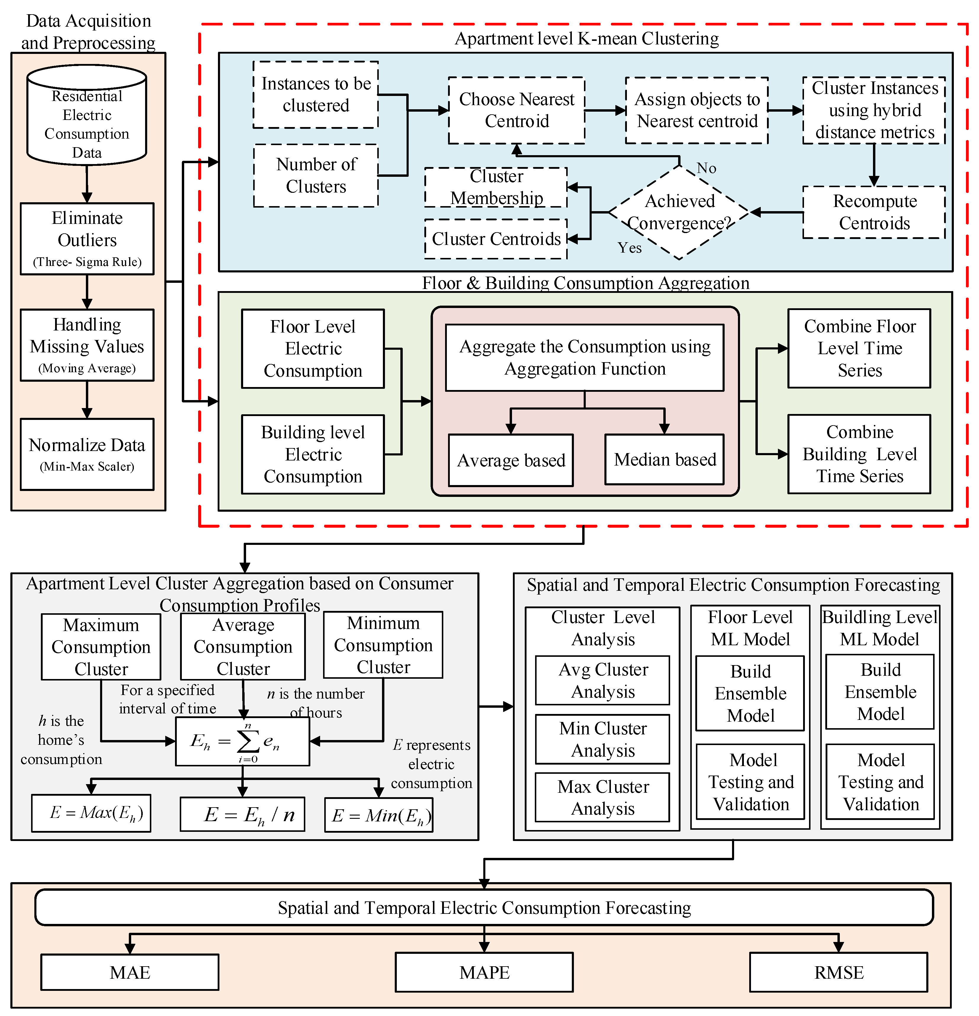
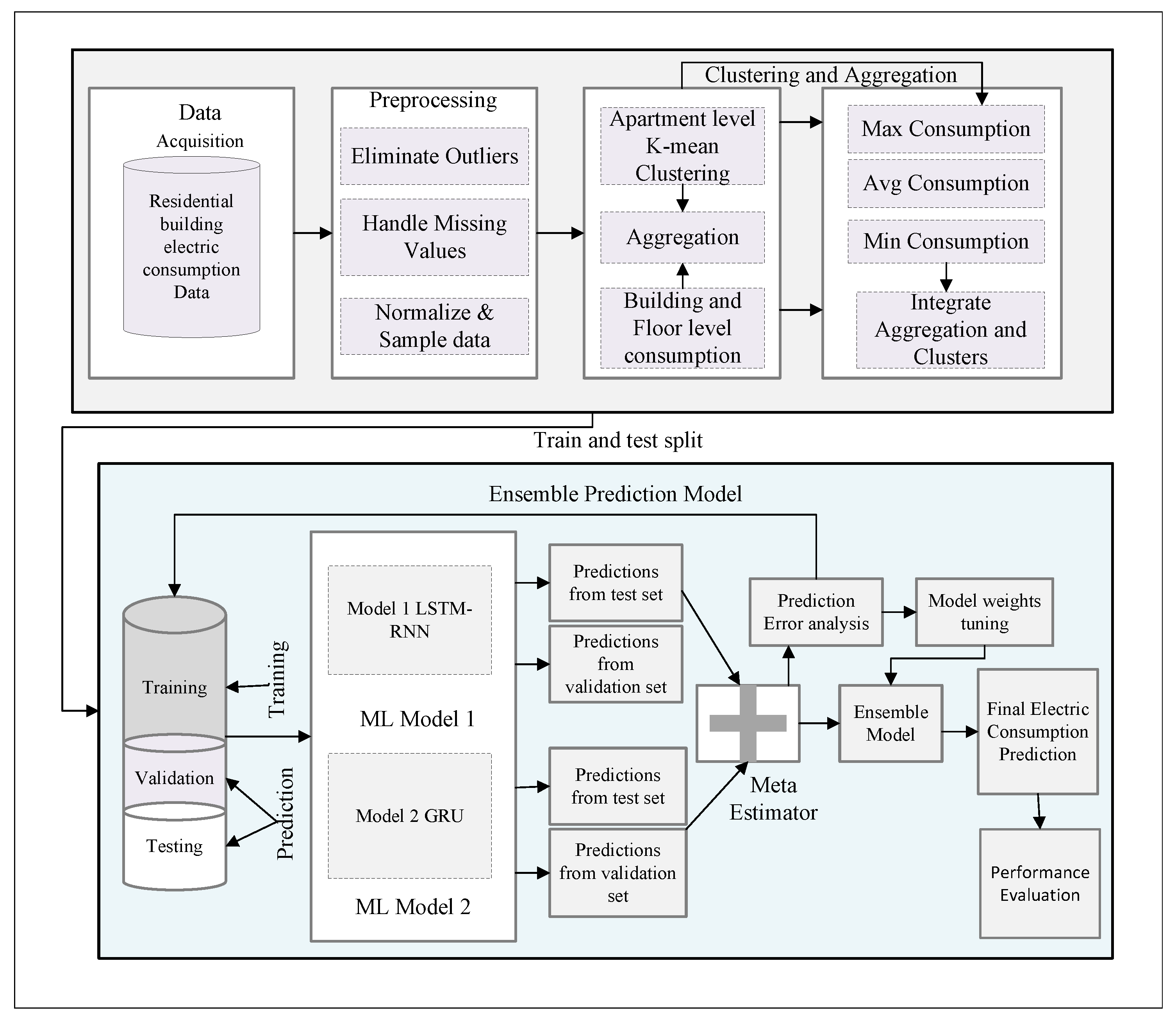
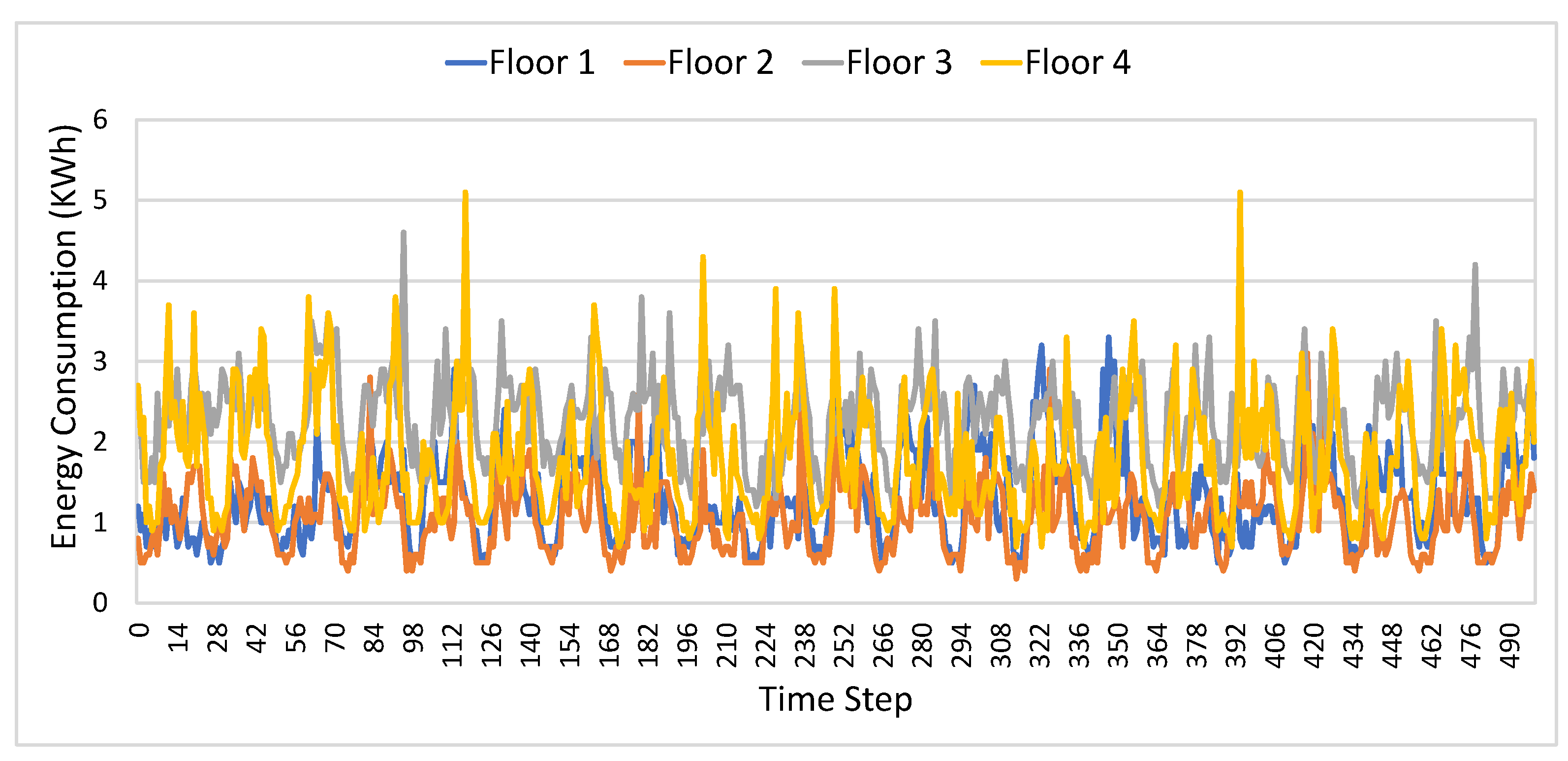
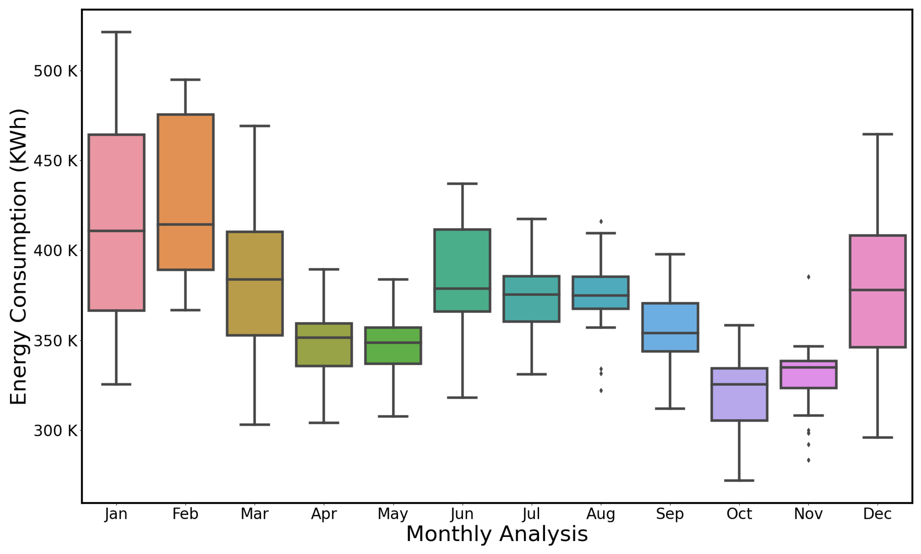
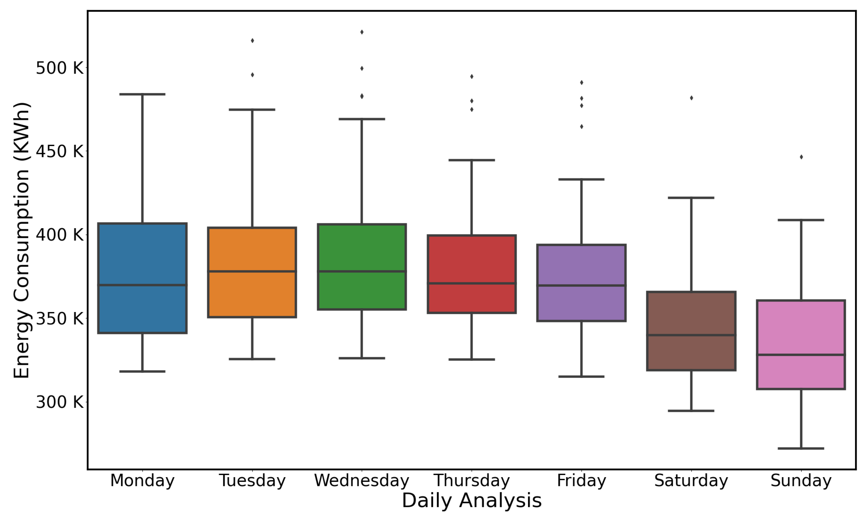
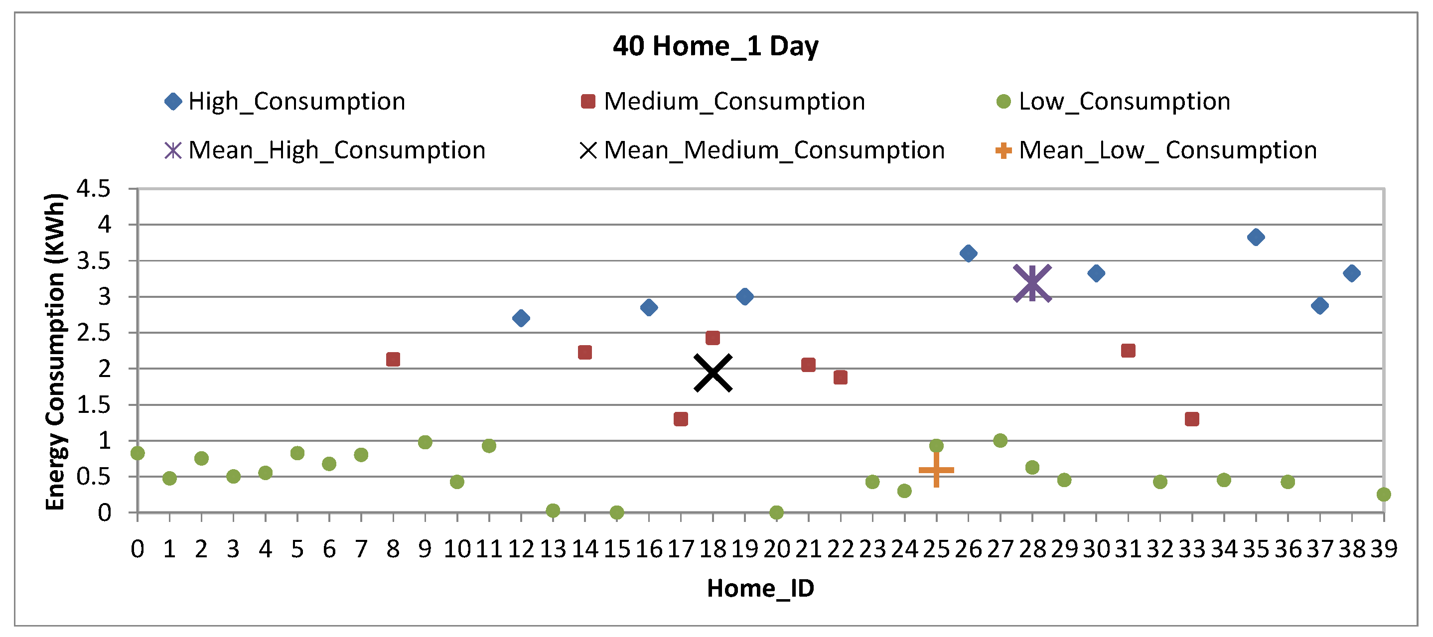
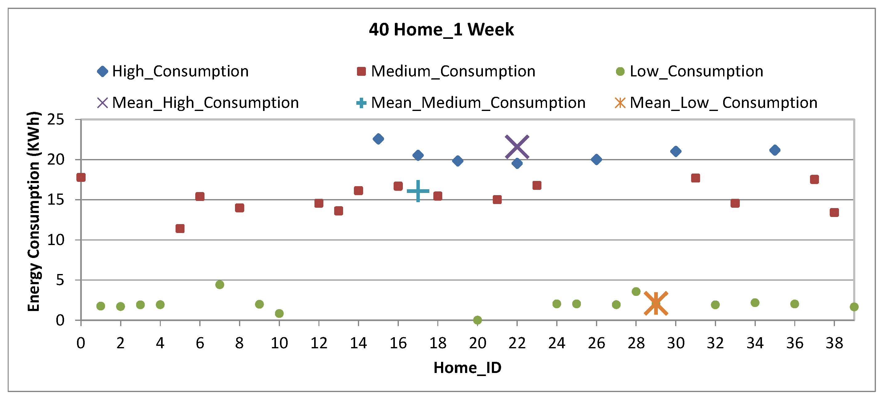
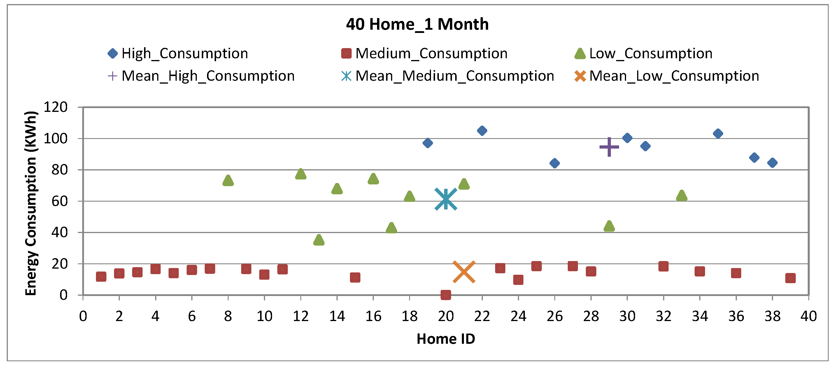
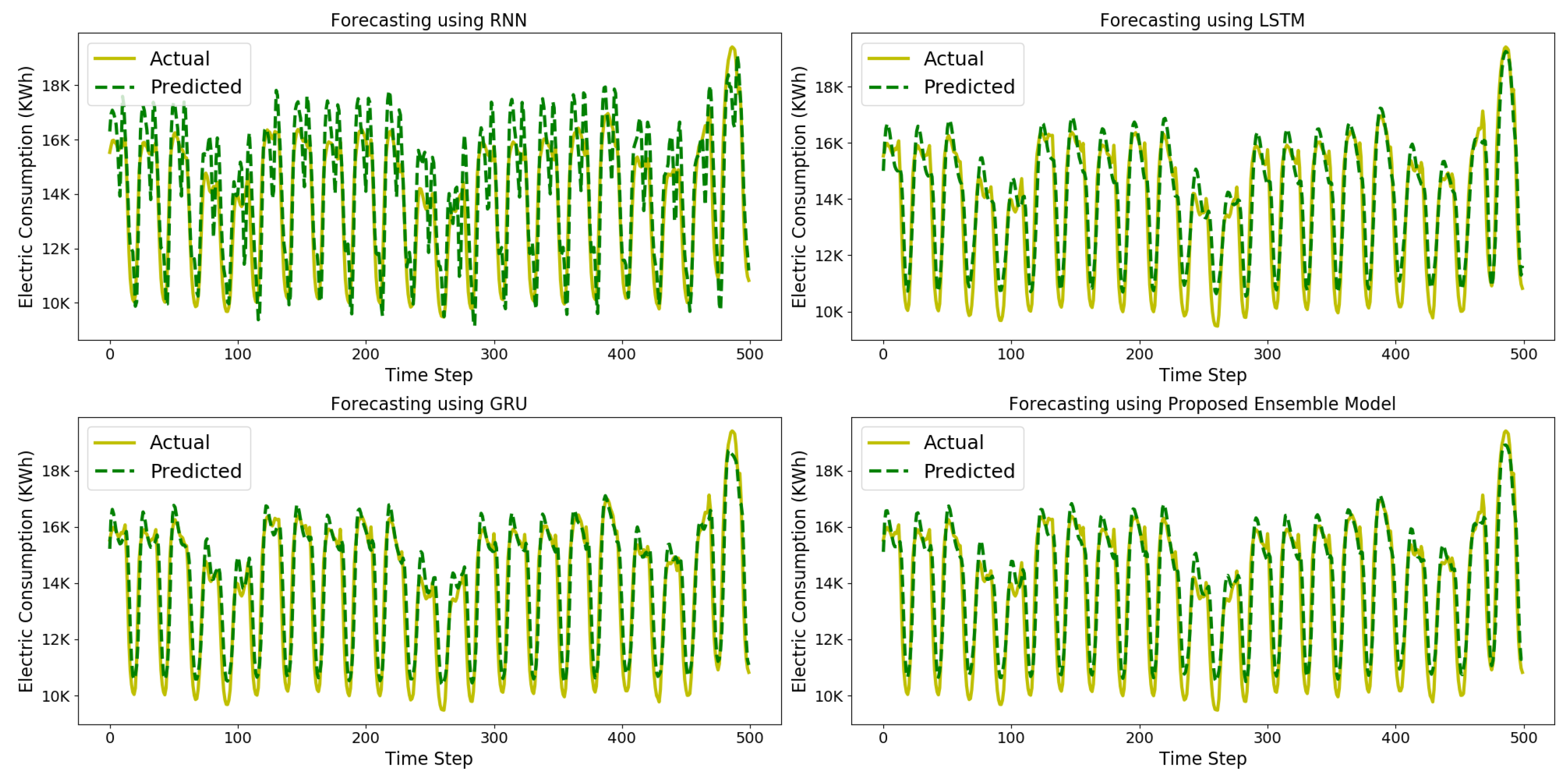
Table 1.
Experimental environment of the proposed spatial and temporal ensemble forecasting model.
| Components | Description |
|---|---|
| OS | Microsoft Windows 10 (64-bits) |
| Processor | Intel ®Core ™ i5-4300 CPU at 3.40 GHz |
| Main Memory | 16 GB |
| Programming Language | Python |
| Flowchart Maker | MS Visio |
| Persistence Storage | MySQL |
| IDE | PyCharm Professional |
| Core Libraries | Numpy, Pandas, Seaborn, Sklearn, Keras, and TensorFlow |
Table 2.
Statistical analysis of proposed ensemble approach with conventional time-series models for hourly electric consumption Forecasting on building level.
Table 2.
Statistical analysis of proposed ensemble approach with conventional time-series models for hourly electric consumption Forecasting on building level.
| Model | MAE | RMSE | MAPE | R2 Score |
|---|---|---|---|---|
| RNN | 1134.191 | 1402.722 | 7.721 | 0.798 |
| LSTM | 786.553 | 981.524 | 5.88 | 0.901 |
| GRU | 709.54 | 907.904 | 5.02 | 0.916 |
| Bi-LSTM | 856.249 | 1040.048 | 6.16 | 0.889 |
| Proposed Model | 572.693 | 737.369 | 4.182 | 0.944 |
Table 3.
Statistical analysis of proposed ensemble approach with conventional learning models for hourly electric consumption forecasting on building level.
Table 3.
Statistical analysis of proposed ensemble approach with conventional learning models for hourly electric consumption forecasting on building level.
| Model | MAE | RMSE | MAPE | R2 Score |
|---|---|---|---|---|
| RF | 2673.256 | 3210.105 | 17.56 | 0.065 |
| XGBoost | 2659.35 | 3208.967 | 17.82 | 0.066 |
| AdaBoost | 2783.009 | 3307.264 | 17.84 | 0.007 |
| GB | 2718.561 | 3242.257 | 17.64 | 0.046 |
| Proposed Model | 572.693 | 737.369 | 4.182 | 0.944 |
Table 4.
Comparative analysis of proposed ensemble model with DELM, ANFIS, ANN, RNN on Daily and Weekly Floor level prediction.
Table 4.
Comparative analysis of proposed ensemble model with DELM, ANFIS, ANN, RNN on Daily and Weekly Floor level prediction.
| Model | Daily Prediction | Weekly Prediction | ||||
|---|---|---|---|---|---|---|
| MAE | MAPE | RMSE | MAE | MAPE | RMSE | |
| DELM | 2.70 | 4.98 | 0.267 | 2.88 | 6.71 | 0.277 |
| ANFIS | 3.10 | 6.11 | 0.299 | 3.39 | 7.93 | 0.317 |
| ANN | 3.42 | 5.61 | 0.389 | 3.51 | 7.95 | 0.397 |
| Proposed Model | 2.06 | 4.54 | 0.231 | 2.19 | 4.71 | 0.239 |
Table 5.
Comparative analysis of proposed ensemble model with DELM, ANFIS, ANN on daily and weekly apartment level forecasting with clustering.
Table 5.
Comparative analysis of proposed ensemble model with DELM, ANFIS, ANN on daily and weekly apartment level forecasting with clustering.
| Model | Daily Prediction | Weekly Prediction | ||||
|---|---|---|---|---|---|---|
| MAE | MAPE | RMSE | MAE | MAPE | RMSE | |
| DELM | 4.60 | 6.43 | 0.310 | 5.00 | 6.99 | 0.356 |
| ANFIS | 5.61 | 9.59 | 0.351 | 5.76 | 8.55 | 0.411 |
| ANN | 5.99 | 10.11 | 0.360 | 6.11 | 9.12 | 0.418 |
| Proposed Model | 3.87 | 5.14 | 0.306 | 4.11 | 6.00 | 0.319 |
Table 6.
Comparative analysis of proposed ensemble model with DELM, ANFIS, ANN on daily and weekly apartment level forecasting without clustering.
Table 6.
Comparative analysis of proposed ensemble model with DELM, ANFIS, ANN on daily and weekly apartment level forecasting without clustering.
| Model | Daily Prediction | Weekly Prediction | ||||
|---|---|---|---|---|---|---|
| MAE | MAPE | RMSE | MAE | MAPE | RMSE | |
| DELM | 10.27 | 15.11 | 4.670 | 13.45 | 19.01 | 4.980 |
| ANFIS | 16.12 | 20.98 | 5.620 | 18.94 | 25.56 | 6.010 |
| ANN | 19.45 | 24.26 | 5.890 | 20.22 | 29.98 | 6.140 |
| Proposed Model | 9.99 | 12.76 | 3.990 | 11.32 | 13.43 | 4.520 |
Table 7.
Comparison of the proposed ensemble model with state-of-art techniques (using same multi-residential buildings data).
Publisher’s Note: MDPI stays neutral with regard to jurisdictional claims in published maps and institutional affiliations. |
© 2021 by the authors. Licensee MDPI, Basel, Switzerland. This article is an open access article distributed under the terms and conditions of the Creative Commons Attribution (CC BY) license (https://creativecommons.org/licenses/by/4.0/).
Share and Cite
MDPI and ACS Style
Khan, A.-N.; Iqbal, N.; Rizwan, A.; Ahmad, R.; Kim, D.-H. An Ensemble Energy Consumption Forecasting Model Based on Spatial-Temporal Clustering Analysis in Residential Buildings. Energies 2021, 14, 3020. https://doi.org/10.3390/en14113020
AMA Style
Khan A-N, Iqbal N, Rizwan A, Ahmad R, Kim D-H. An Ensemble Energy Consumption Forecasting Model Based on Spatial-Temporal Clustering Analysis in Residential Buildings. Energies. 2021; 14(11):3020. https://doi.org/10.3390/en14113020
Chicago/Turabian StyleKhan, Anam-Nawaz, Naeem Iqbal, Atif Rizwan, Rashid Ahmad, and Do-Hyeun Kim. 2021. "An Ensemble Energy Consumption Forecasting Model Based on Spatial-Temporal Clustering Analysis in Residential Buildings" Energies 14, no. 11: 3020. https://doi.org/10.3390/en14113020
Note that from the first issue of 2016, this journal uses article numbers instead of page numbers. See further details here.