
Large-Eddy Simulation Analyses of Heated Urban Canyon Facades


Department of Physics and Astronomy, University of Bologna, via Irnerio 46, 40126 Bologna, Italy
*
Author to whom correspondence should be addressed.
Energies 2021, 14(11), 3078; https://doi.org/10.3390/en14113078
Submission received: 18 April 2021
/
Revised: 20 May 2021
/
Accepted: 22 May 2021
/
Published: 25 May 2021
(This article belongs to the Special Issue Turbulent Flow Simulations: Laboratory and Numerical Modelling of Turbulent Flows)
Abstract
:Thermal convective flows are common phenomena in real urban canyons and strongly affect the mechanisms of pollutant removal from the canyon. The present contribution aims at investigating the complex interaction between inertial and thermal forces within the canyon, including the impacts on turbulent features and pollutant removal mechanisms. Large-eddy simulations reproduce infinitely long square canyons having isothermal and differently heated facades. A scalar source on the street mimics the pollutant released by traffic. The presence of heated facades triggers convective flows which generate an interaction region around the canyon-ambient interface, characterised by highly energetic turbulent fluxes and an increase of momentum and mass exchange. The presence of this region of high mixing facilitates the pollutant removal across the interface and decreases the urban canopy drag. The heating-up of upwind facade determines favourable convection that strengthens the primary internal vortex and decreases the pollutant concentration of the whole canyon by compare to the isothermal case. The heating-up of the downwind facade produces adverse convection counteracting the wind-induced motion. Consequently, the primary vortex is less energetic and confined in the upper-canyon area, while a region of almost zero velocity and high pollution concentration ( more than the isothermal case) appears at the pedestrian level. Finally, numerical analyses allow a definition of a local Richardson number based on in-canyon quantities only and a new formulation is proposed to characterise the thermo-dynamics regimes.
1. Introduction
The ongoing worldwide urbanisation and increasing population of the urban environments have raised awareness towards a series of environmental issues having adverse effects on public health [1,2]. Air pollution due to vehicular emissions is recognised as one of the major health threats [3], as a consequence of a large number of sources in a poorly ventilated environment and high level of exposure for the urban residents [4,5,6]. Understanding the flow circulation and ventilation within the urban canopy is paramount to predicting population exposure and developing solutions to improve residents’ livability and comfort, thus requiring a morphology revision of the canopy environment [7] or the introduction of novel techniques to reduce pollutant concentrations [8].
Most of the recent investigations on the flow circulation and ventilation processes in urban canopies have delved into the characterisation of the inertial flow regime under isothermal conditions (i.e., driven by the mechanical force exerted by the free-stream wind velocity above the canopy) and less so on the thermal effects. Thermal stratification and convection are caused by the buoyancy force induced by differential surface heating by solar irradiation and contribute to the modification of the canopy flow and turbulent regimes, especially under weak inertial forcing [9]. The horizontal temperature gradient establishing between differently heated building facades forces a thermally-driven circulation within the canopy that can modify or superimpose the already-established inertially-driven vortex [9,10,11,12,13]. Contextually, turbulent energy and momentum transport is also modified [14,15,16,17], playing a significant role in the canyon pollutant dispersion and scalar mixing [17,18]. Additional buoyancy forces arise from the street and building surfaces [19] and rooftop heating [20], enhancing the convective forcing according to the solar path [14,21], and thus modifying the heat transfer [22] and thermally-related ventilation [23]. Boundary-layer unstable stratification further enhances the in-canyon ventilation due to the interaction of the canopy vortex with the large convective eddies above [24].
Different non-dimensional coefficients have been introduced to discern inertial from thermal flow regimes within an urban canyon. Among others, Dallman et al. [9] derived a buoyancy parameter as the ratio between buoyancy force generated by opposite building facades at different surface temperature and the free-stream velocity to determine if the in-canyon circulation is inertially or thermally driven. Magnusson et al. [11] refined this parameter by further characterising the mixed-phase condition, where both mechanical and thermal forces impact the observed circulation. Most commonly, the canopy-flow regimes are investigated in terms of a bulk Richardson number
where g is the gravity acceleration, is the thermal expansion coefficient, is the characteristic temperature difference, H is the mean building height, and free-stream velocity. Such a quantity compares the buoyancy force per unit mass between canyon surfaces (e.g., street, building facades, rooftops) with the wind-driven mechanical force per unit mass . The results of the buoyancy–mechanical force balance is oftentimes addressed in terms of convection regimes. For , the in-canyon flow regime is inertially-driven and convection is suppressed (forced convection regime), while for both thermal and inertial forces become significant (mixed convection regime). The third regime of natural convection is obtained at 1 when buoyancy force dominates inertia (condition typically achieved under wind calm). Unlike the buoyancy parameter, the Richardson number does not have precise thresholds, but the convective regimes seem to depend on local atmospheric and morphology conditions. For instance, Li et al. [25] observed a direct transition between forced and natural convection at ∣ 20 in asymmetric urban canyons while Allegrini et al. [26] observed a mixed-phase at 1.
In the context of non-isothermal urban canyon flows, the use of non-dimensional parameters provides a useful tool to discern the mechanical and thermal force balance. However, the characteristic temperature difference and free-stream velocity required by the Richardson number are not unequivocally determined in the literature, somehow limiting the comparability between different studies. As revealed by Zhao et al. [27], the characteristic temperature difference has been computed between the air at the rooftop and street level, windward and leeward building facades or a heated surface and ambient air, thus limiting the inter-study comparability. Moreover, in field experiments the canyon and above atmosphere are rarely isothermal; thus, the ambient temperature is a critical parameter too. This aspect is typically overtaken in the laboratory and numerical experiments where an isothermal ambient flow is perturbed by heating a target surface. The free-stream velocity is also not unequivocally determined: if in field studies the computation of this quantity undergoes the limitation of the instrumental arrangement (i.e., how above the canyon we have managed to install an anemometer), there is not a unique definition for laboratory and numerical studies.
A limited number of studies have used the convective-regime classification given by the Richardson number to investigate the buoyancy force and thermally-driven flows in urban canyons, with no definitive conclusions on their impact on the observed regimes. Given the flow inertia, the intensity and direction of the buoyancy force have determined an intensification/enlargement or weakening/shrink of the inertial vortex [28,29], or the formation of one/more counter-rotating vortex/vortexes both from field measurements [30] and numerical simulations [31]. However, in the same study by Louka et al. [31], a single recirculation vortex has been observed from field data, with the heating effect of the building facade being confined in a thin layer close to the same building. This second outcome is in agreement with other studies (e.g., [14,32,33,34]) which only observed an intensification of the upwards motion at the heated facade. Xie et al. [35] also found that an increasing aspect ratio leads to the formation of multiple vortexes within the canyon, in contradiction to Magnusson et al. [11] where the number of vortexes decreased to only one when introducing a buoyancy force.
The present study aims at providing further insight into the mixed-convection regime of a single infinitely-long urban canyon of unity aspect ratio. This study will delve into the thermo-fluid dynamics and turbulence of the in-canyon region and impacts on the pollutant removal, as obtained from a stationary background flow and varying buoyancy forces. Thus, we will not explore the full extent of the boundary-layer processes above it nor the variations in the background flow structure. Highly-resolved large-eddy simulations (LESs) are employed to reproduce the non-linear interaction among the in-canyon inertial velocities induced by the surrounding flow, the natural convection arising from heated building facades, and the mechanisms of pollution removal. Numerically, this required a careful choice of numerical schemes to realistically reproduce the coupling between inertial and thermal turbulence. Physically, the simultaneous presence of these elements generates complex thermo-fluid dynamics and turbulence features which are analysed in details. Also, the in-canyon flow regimes are investigated to further characterise the potential issues related to pollutant concentration removal and pedestrian exposure.
This paper is organised as follows: Section 2 describes the case study of this investigation, while Section 3 is devoted to the numerical simulation approach adopted. In Section 4 the simulation settings are presented leading to the simulation-approach validation in Section 5. Section 6 provides the major results of this investigation. Finally, Section 7 draws the conclusions.
2. Case Study Description
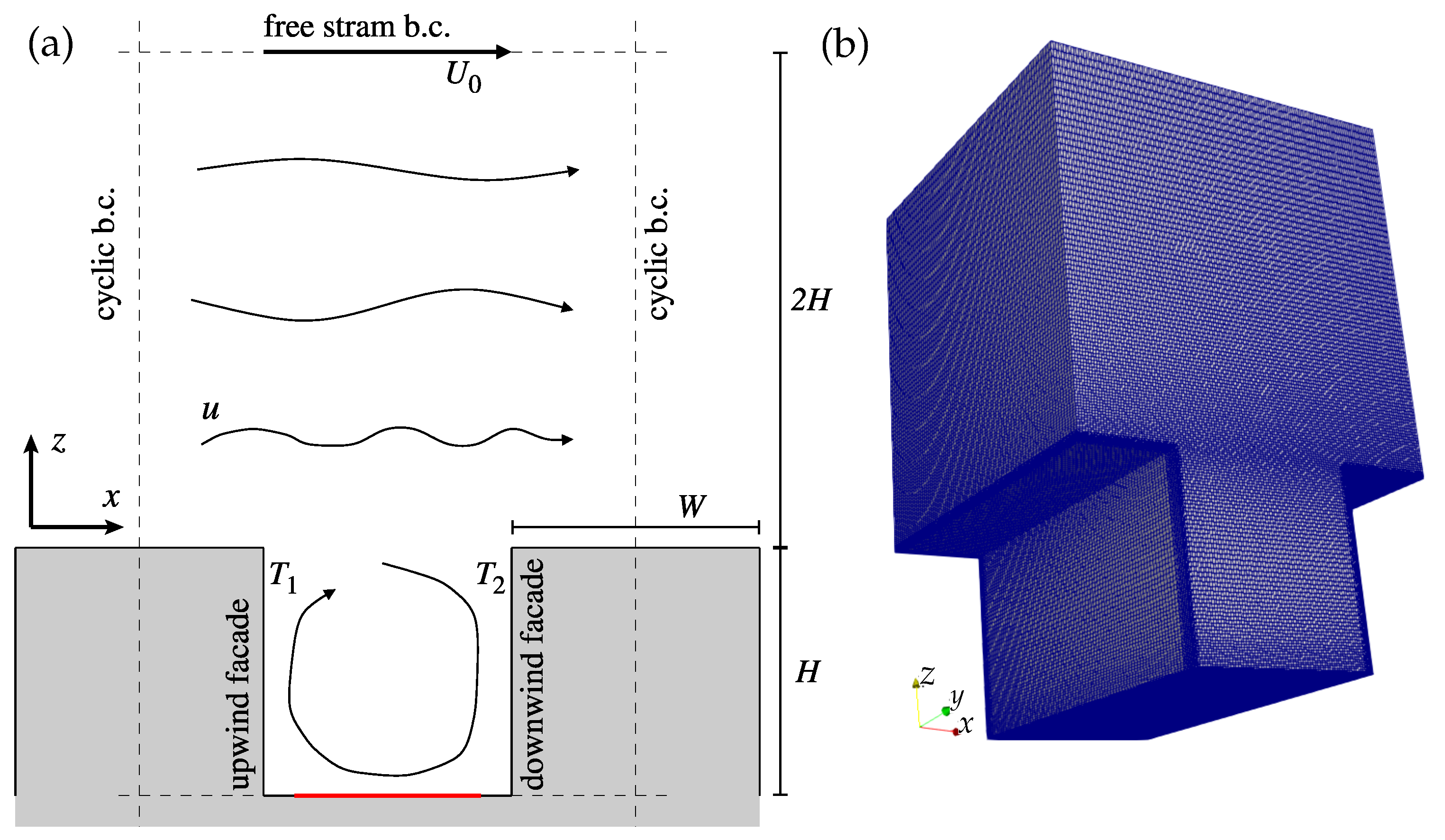
Numerical simulations reproduce the paradigmatic case of periodic arrays of infinitely long square canyons. The ambient wind is perpendicular to the canyon axis. A pollutant concentration is released from the bottom of the canyon with constant flux, while the facades of the buildings bordering the canyon heat up differently and generate natural convective motions (see Figure 1a). Two cases are analysed: (1) the favourable convection case, where the upwind facade is heated up and the other surfaces are at ambient temperature. In such a case, the convective velocity supports the velocity induced by ambient wind and the in-canyon circulation is strengthened. (2) The adverse convection case, where the downwind facade is heated up and the other surfaces are at ambient temperature. In this case, the convection flow opposes the ambient-induced velocity and the overall internal circulation is altered. The neutral case, where all the solid surfaces are at ambient temperature, is also reported as a reference.
Figure 1 displays the case study geometry and computational domain dimensions. Two square buildings of height m and width m delimit a canyon with an aspect ratio . The computational domain consists of a rectangular region that is wide (centred in the canyon), height (starting from the bottom canyon level), and deep along the canyon axis direction which is a direction of flow homogeneity. Since the attention is focused on the in-canyon dynamics, the height of the domain has been limited to following the example of similar studies [36,37]. The origin of the system of reference is placed at the bottom left corner of the computational domain; the vertical, streamwise and spanwise direction are the z, x and y direction, respectively.
The ambient flow is perpendicular to the canyon axis, i.e., directed in the x-direction, and the average free-stream velocity at the top boundary is . The source of pollutant concentration c is at the street level, in a region large and centred in the canyon. Such a region delimited the carriageway where motor vehicles release pollutant and do not extend the full width of the canyon to account for the presence of footpaths. The natural convection arises at the vertical building facade within the canyon. The buildings are at ambient temperature, while the temperature of the upwind facade () and downwind facade () are changed to produce two different horizontal thermal gradients. It should be noticed that in real case configurations, also the building roofs and the street can be heated up by solar radiation. Possibly, a mixed configuration where the rooftop, one building facade and the street are heated up, is also more common. The present study aims to analyse the effects of a horizontal thermal gradient, while additional setups can be investigated in future dedicated studies.
Non-Dimensional Parameters
The ambient wind fluid dynamics is characterised by the Reynolds number based on building height:
where is the kinematic viscosity of air. The natural convection is described by the Grashof number, which is the ratio between the buoyancy force and the viscous force:
The Richardson number can be interpreted also as the ratio of the buoyancy term to the flow shear term, and it is introduced to state the relative importance of the buoyancy force and the atmospheric wind:
where is the characteristic buoyancy velocity. Additional parameters are the Prandtl number , the ratio between kinematic viscosity and thermal conductivity, and the Schmidt number , the ratio between the kinematic viscosity and concentration diffusivity.
Quantities are made non-dimensional by means of the buildings height H for length and the free stream velocity for velocities. The ambient flow time scale is defined as . Temperature is normalised as where is the ambient reference temperature and is the difference of temperature between the two building facade. Concentration is made non-dimensional as and the reference concentration is defined from the concentration flux at the street level , where is the molecular diffusivity and n is the street-normal direction (see also Section 4.3).
3. Simulation Approach
The thermo-fluid dynamics proprieties of air are summarised in Table 1. The modelling approach is detailed in the following sections.
3.1. Mathematical Model
The air is modelled as an incompressible fluid and the Boussinesq approximation is adopted to account for the buoyancy force. The governing equations read:
where are the velocity components (), is the deviation from the kinematic hydrostatic pressure, is the gravity acceleration vector, T is temperature, is the molecular thermal conductivity, and are the reference density and temperature, respectively. The pollutant concentration is modelled as follows:
with the molecular pollutant diffusivity. Being a passive scalar, c is just advected and diffused by the flow.
3.2. Large-Eddy Simulation Approach
In the LES approach, the scales of motion larger than the computational cell width are directly resolved, while the smallest scales are modelled (for example see Rodi et al. [38]). The numerical resolution of the governing equations over a discrete mesh acts as an implicit spatial filter (denoted with an overlying bar), which decomposes the velocity field in a filtered and a residual component: . Applying the filter to momentum Equation (6), an extra term appears and is modelled through the dynamic Lagrangian model proposed by Meneveau et al. [39]. Details on the mathematical model implemented can be found in Cintolesi et al. [40] and are not here reported for the sake of conciseness. Such a model is particularly suitable for reproducing localised and anisotropic turbulence because it can determine the sub-grid scale (SGS) contribution to the resolved flow at each point of the computational domain, extracting information from the instantaneous velocity field. Hence, this is convenient for simulating the present case, where the largest part of the turbulent motion is localised at the canyon-atmosphere interface. It was also shown that it can adjust the value of the SGS viscosity near the solid boundaries, overcoming a well know shortcoming of the Smagorisnky model which uses damping function as the Van Driest function [41] to correctly reproduce the turbulent energy dissipation near walls [39]. Moreover, the empirical content and case-dependency of the model are reduced, since the value for the model parameter is not specified as in the original Smagorinsky model but inherently computed.
A model for SGS contribution is also required for temperature and concentration. When the implicit spatial filter is applied to temperature Equation (7), a SGS thermal flux appears and is modelled by the flux-gradient hypothesis:
where the last equation is the flux-gradient model and is the sub-grid scale thermal diffusivity. This is expressed using the Reynolds analogy as , where is the turbulent Prandt number. In a very similar way, the filtering of the concentration Equation (8) leads to a SGS concentration flux and a SGS pollutant diffusivity that is computed as , with the turbulent Schmidt number. Additional details on the SGS model for active and passive scalar are reported in Cintolesi et al. [42,43].
3.3. Algorithm and Numerical Schemes
The numerical simulations are carried out using OpenFOAM [44], open-source software for computational fluid dynamics. The solver pimpleFoam has been customised to include the resolution of temperature and concentration Equations (7) and (8). The SGS model described in Section 3.2 has been originally implemented and tested in several previous studies [40,43,45].
The solution algorithm is the Pressure-Implicit with Splitting of Operators (PISO) as it is implemented in OpenFOAM (see the software documentation [44]). The buoyancy term in momentum Equation (6) is added as an explicit source term. The discretisation schemes are of the second-order accuracy: the implicit Euler backward scheme is used for time derivative, the central-difference scheme is used for spatial derivative. To stabilised the simulation, the convective term in temperature and concentration equations are discretised using the Gauss–Gamma scheme () proposed by Jasak et al. [46], which is a bounded central-difference scheme based on the normalised variable diagram. A numerical clipping is enforced on T and c to prevent nonphysical values given by numerical instabilities. The clipping acts on a limited number of computational cells during the initial development of the flow and once the statistically steady state is reached, it is practically not activated.
4. Case Settings
This section reports the numerical settings of the cases under consideration, along with the physical parameters adopted and compared with typical field-experiment values.
4.1. Physical Parameters Set-Up in View of Field-Experiment Evidences
Table 1 summarises the non-dimensional numbers that characterised the flow regime, together with the characteristic velocity and temperature difference, and the physical parameters adopted in this investigation. The Reynolds number based on the building high is set to be which is larger than the critical value ensuring the fluid-dynamic Reynolds independence for square urban canyons [47,48]. Thus, the velocity field (suitably scaled) reproduces the same configuration obtained at higher that are characteristic of real atmospheric conditions. Nevertheless, caution should be paid on this point since no studies have verified the validity of the criterion of independence of the motion from Reynolds number in the presence of natural convection. The temperature gradient imposed between the two vertical building facades is set to be K, leading to a Grashof number , indicating that the convective flow along the vertical building surfaces is in a turbulent regime. The Richardson number is suggesting that convective forces introduce non-negligible effects in the overall circulation.
The physical parameters for this case study are derived because of evidence from several field experiments devoted to the investigation of convective forces in urban canyons. Table 2 summarises the typical values of Reynolds, Grashof and Richardson numbers in several urban canopies subjected to different free-stream velocities and temperature differences. Field studies encompass real cities and controlled environments (e.g., ad-hoc canopies build with containers or homogeneous concrete bodies positioned in unperturbed open spaces), with different mean building heights H and aspect ratios . It is paramount to be aware that free-stream velocity and temperature differences are not equally determined in these studies due to the diverse instrumentation equipment and setup of the field experiments. The free-stream velocity is defined as the speed of the background flow unperturbed by the canopy. This measurement is not commonly available in an urban environment, where is typically replaced by the wind speed measured at the highest available instrumented level above the canyon, which is necessarily different in each selected study. Conversely, the identification of the temperature difference is a matter of various definition adopted by individual authors. The is estimated using the temperature of a heated surface (e.g., building facades or street) measured with thermocouples or thermo-cameras and a reference air temperature from thermocouples or probes. The major issue with the temperature-difference definition is the computation of the reference air temperature. Most studies [12,13,14,31,49] in Table 2 chose the air temperature measured above the canyon rooftop as the reference (at the same elevation used for measuring the free-stream velocity). The remaining studies [30,34,50] in Table 2 used the mean canyon temperature as the reference. These differences open up a discussion on the necessity to define a clear and unique Richardson number, suitable for real urban environments where the canopy and the surrounding atmosphere are rarely isothermal. The absence of consensus leads to ambiguities in the set-up of physical and non-dimensional parameters for studying urban canyon flows, limiting the research comparability. Compared to Table 2, the Richardson number used in the present study is within the typical range observed in field experiments, while Reynolds and Grashof numbers are smaller by orders of magnitudes, which is due to the reduced ambient wind velocity and building height compare to real case settings.
4.2. Computational Domain
The computational domain is discretised with an unstructured and staggered mesh, which is depicted in Figure 1b. The mesh consists of 1,592,562 cells; it is refined near the solid boundaries to ensure the direct resolution of the wall boundary layer and slightly stretched near the canyon-atmosphere interface () where high turbulent motions are expected [40]. Preliminary simulations showed that the first computational point near the walls is placed within (note that to maintain the traditional notation, here y is the wall-normal coordinate and is the friction velocity); thus, the wall boundary layer is well resolved [51]. Also, the adequacy of spatial discretization was checked: an additional simulation has been performed over a finer grid having more cells in all directions. The first- and second-order statistics of velocity field along selected lines, computed using the present and the refined mesh, do not show differences. The time steps are dynamically computed to ensure the maximum Courant-Friedrichs-Lewy number , which preserves the numerical stability and accuracy (e.g., Trivellato and Raciti Castelli [52]).
4.3. Initial and Boundary Conditions
The flow is driven by a pressure gradient dynamically computed in a way that the average streamwise velocity at the top boundary is maintained at a fixed value . At the top boundary, the zero-gradient conditions are prescribed for velocity and temperature, while a zero value is set for pressure and concentration. These conditions mimic a free interface that allows the removal of pollutant and temperature from the domain. At solid walls, a non-slip condition is enforced for velocity and zero-gradient is imposed to pressure. The pollutant is released at the canyon street level () in the area , corresponding to the carriageway for motorcycles. In this area, it is imposed a constant flux of concentration , where n is the street-normal direction. At the remaining solid boundaries, a zero-gradient condition is imposed. Regarding temperature, different constant values are set at the various walls: the horizontal boundaries are at the atmospheric temperature (building roof and canyon street); the vertical boundaries composed by the upwind () and downwind () building facade have a fixed temperature and respectively (see Figure 1). In the favourable convection case, the upwind facade is heated up at while the downwind facade is at ambient temperature . Conversely, in the adverse convection case, the upwind facade is at ambient temperature and the downwind facade is at . Lastly, an isothermal configuration is imposed in the neutral case. The computational domain is made virtually infinite in the y direction and periodic in the x direction, by imposing a cyclic boundary condition for all variables.
The initial conditions are constant weak streamwise velocity m/s and zero values for others quantities. To accelerate the development of the flow dynamics, a preliminary simulation has been run to reach the statistical steady state for velocity and pressure, without resolving the temperature and concentration fields. Subsequently, the temperature and concentration have been transported as a passive scalar by an instantaneous configuration of the velocity field. Finally, the resolution of the complete model is activated and the coupling set of equations are resolved till a statistical steady state configuration is reached, after which the statistics are collected for a period of non-dimensional time.
Statistics are computed by averaging in time (over a period of ) and along the spanwise direction (y, which is a direction of homogeneity). The average in time and space of a generic variable is denoted by angular bracket ; the fluctuations are denoted ; the root-mean-square (RMS) are indicated and computed as .
5. Simulation Approach Validation
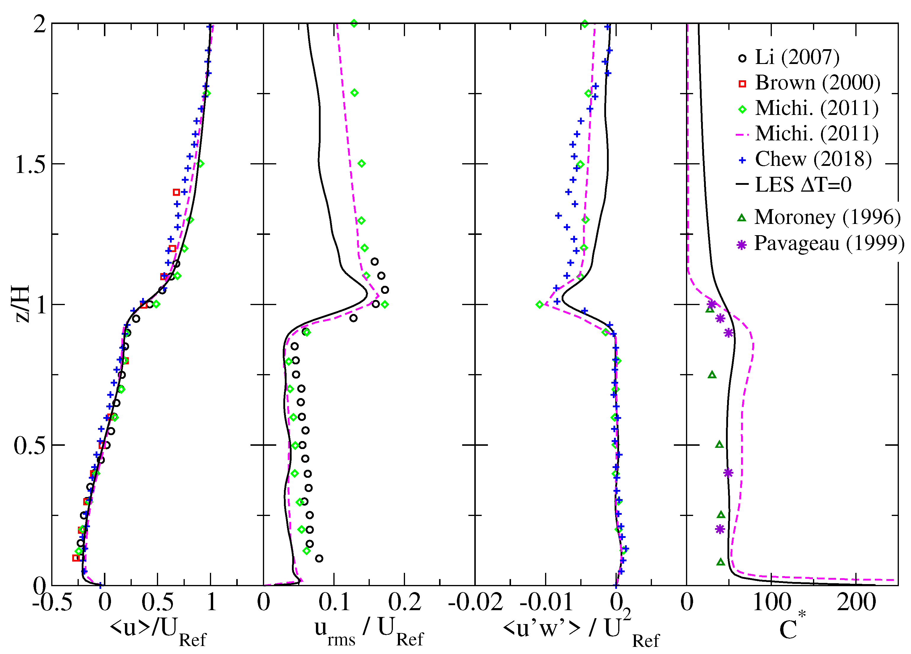
The accuracy of the simulation approach and the numerical solver has been assessed in Cintolesi et al. [40]. The neutral case, i.e., in absence of a temperature gradient and natural convection, has been reproduced and successfully validated against several experimental and numerical results from the literature. For the sake of completeness and to make this study as self-consistent as possible, the validation of the neutral case is here briefly reported and discussed. The simulation has been validated against laboratory experiments and one numerical simulation reported in the literature. Five datasets have been used for the comparison: Li et al. [36] and Chew et al. [48] perform a water-channel experiment considering seven canyons, collecting measurements at the central canyon. The former uses a two-colour laser Doppler anemometer, the latter uses an acoustic Doppler velocimeter with a sampling volume of m . Brown et al. [53] used a wind tunnel with six canyons and take the measurements with a pulsed-wire anemometer at the 3rd–4th canyons, where the flow reaches the equilibrium. Michioka et al. [47] perform a laboratory experiment in a wind tunnel with 24 canyons, collecting velocity measurements with a laser Doppler velocimeter. They also present an LES provided with the dynamic SGS model proposed by Germano [54] and Lilly [55]. Meroney et al. [56] and Pavageau and Schatzmann [57] provide concentration profiles obtained in laboratory experiments.
Figure 2 shows first- and second-order statistics for the streamwise velocity and the mean concentration profile along the canyon vertical centerline (). To be consistent with the reference datasets, the velocity has been made non-dimensional through m/s, which is the mean streamwise velocity at the height of . The profiles of the mean streamwise velocity collapse to the same line, while the RMS profile slightly underestimates the resolved fluctuations predicted by the experiments but is in agreement with the simulation of Michioka et al. [47]. The peak of the resolved turbulent kinematic momentum fluxes at the canyon-atmosphere interface () is lightly weaker, while the pollutant concentration within the canyon is satisfactorily reproduced. Given the validation performance, the simulation approach is considered adequate to reliably reproduce the case study under investigation.
6. Results
The three introduced configurations are herein numerically reproduced and discussed. The neutral case where the building facades are at the same ambient temperature and therefore no natural convection is generated. The favourable case where the upwind building facade is heated up and the convective motion develops in the same direction of the inertially-driven motion of the principal vortex within the canyon. The adverse case where the downwind building facade is heated up, triggering a vertical convective velocity that opposes the motion of the main canyon vortex generated by the overlying ambient wind. See Section 4.3 for a complete description of the numerical settings.
6.1. Overall Canyon Dynamics
A first insight into the general circulation within the canyon is given through the spatial distribution of the principal variables (averaged and made non-dimensional) at a vertical plane . A quantitative analysis is reported in the subsequent Section 6.2.
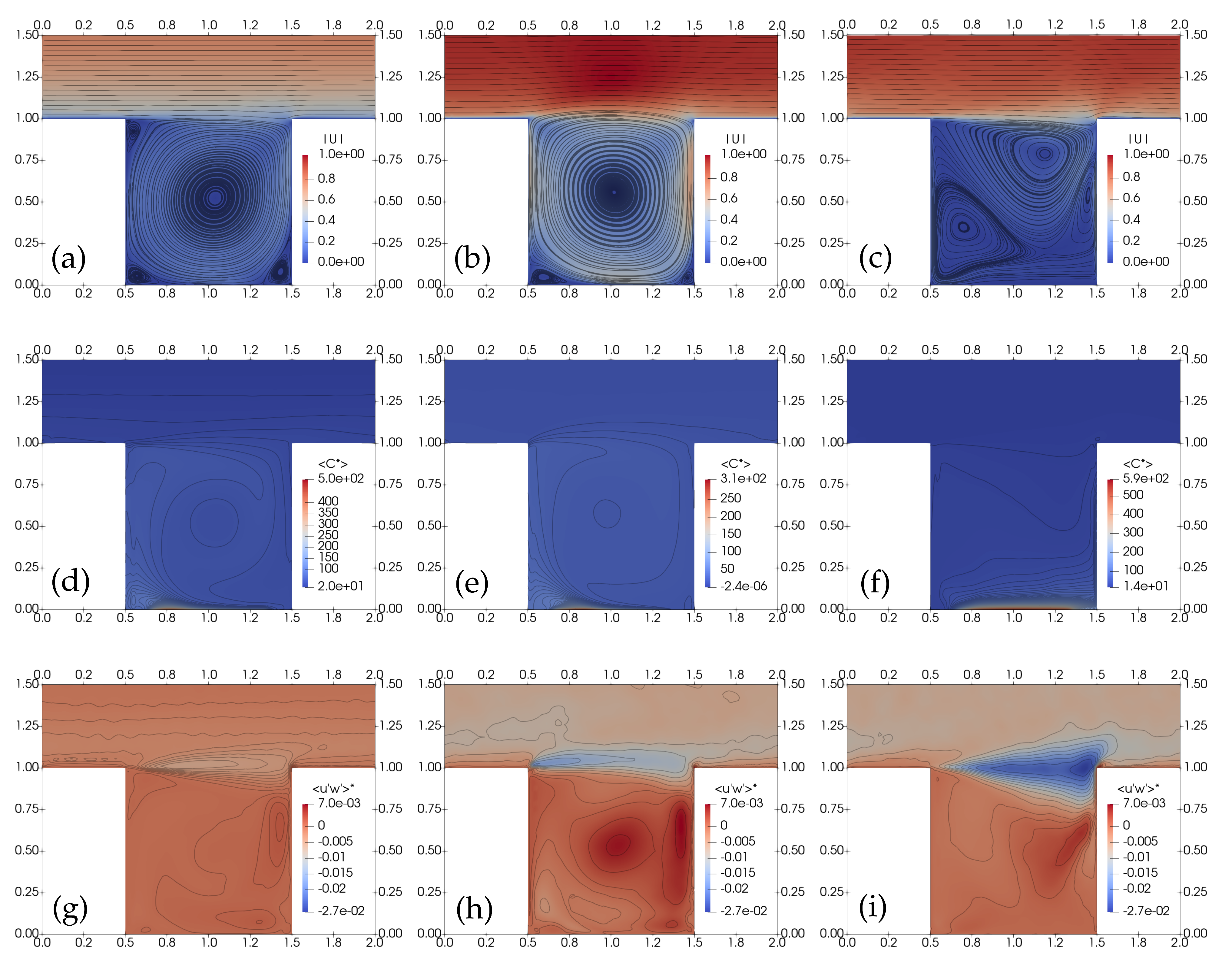
Figure 3a–c shows the velocity streamlines superimposed to the velocity magnitude distributions for the three cases under consideration. The neutral case (Figure 3a) exhibits the typical characteristics of the canyon flow induced by an ambient wind: the clockwise rotating principal vortex and three secondary counterclockwise recirculation regions at the top-left, bottom-left and bottom-right corner of the square canyon. Particularly, the top-left recirculation region is generated by the sharp horizontal shear produced by the ambient wind at the rooftop level. The canyon-ambient interface, defined as the upper boundary of the principal vortex is essentially a horizontal straight line that coincides with the rooftop level . The favourable case (Figure 3b) displays a more intense ascending motion near the upwind facade which, in turn, destroys the top-right recirculation region and bends the interface upward until its climax at and . The contribution of thermal convection impacts the overall canon recirculation, enhancing the primary vortex velocity also near the downwind facade and at the central region of the street while reducing the extensions of the two recirculation regions at the bottom corners. The adverse case (Figure 3c) shows a quite different configuration: the convective velocity at the downwind facade counteracts the downward flow from ambient wind by decreasing its intensity and deflecting its trajectory towards the canyon centre. The result is that the primary vortex is less energetic and confined in the upper-canyon (). The two recirculation regions located in the bottom corners of the canyon increase their extension and are displaced upward, while an area characterised by an almost zero velocity appears at the canyon bottom (), generating a zero-velocity region (see also discussion of Figure 5). The interface is a straight line starting at the upwind building top corner and intercepting the downwind building facade at .
Figure 3d–f reports the pollutant concentration distribution and contour lines. All the cases have a maximum concentration near the street, where the source of the pollutant is located. The neutral and favourable cases (Figure 3d,e) exhibit an accumulation of concentration in the bottom-left corner, in correspondence of the recirculation region, and near the upwind facade as a consequence of the transport by the primary vortex. Instead, the adverse case (Figure 3f) accumulates the larger part of the concentration in the zero-velocity region, while decreasing with an almost vertical gradient. This is due to the thermal stratification which characterises the zero-velocity region, see Figure 4.
Table 3 depicts the distribution of the pollutant concentration within the entire domain, the canyon (), and the zero-velocity region (), using the concentration density and the main recirculation quotient . The concentration density for each region is computed as
where is the volume of the region under consideration; the main recirculation quotient introduced by Göthe et al. [58] is defined as
On average, the concentration density in the domain is higher in the neutral case which is less effective in dispersing the pollutant across the top boundary. Within the canyon, the favourable case shows lower values thanks to the enhanced internal recirculation, while in the zero-velocity region the adverse case exhibits a very high level of concentration. This zero-velocity region approximately coincides with the pedestrian level defined by Buccolieri et al. [59] which corresponds to about 1 to 2 m above the street, and where a high concentration of pollutants particularly affects human health. The main recirculation quotient shows that the neutral and adverse cases are equivalent in the removal of pollutant concentrations from the canyon, with the favourable case being more effective. Also, it points out that in the adverse case the pollutant accumulates near the street, whilst the upper part has a level of concentration similar to the favourable case.
Figure 3g–i shows the turbulent kinematic momentum fluxes. Overall, two principal regions of negative and positive fluxes are common to all the cases:
- The interaction region,
- horizontally elongated and centred at the canyon-ambient interface, where the ambient flow interacts with the canyon recirculation and presents negative turbulent fluxes caused by the presence of ejection and sweep events enhancing mixing and pollutant dispersion.
- The descent-flow region,
- vertically elongated near the downwind facade, where the deflection of the ambient wind triggers a descending flow that enters the canyon and drives the principal clockwise vortex.
The turbulent fluxes are more intense in presence of natural convection which leads to a more energetic internal flow. The neutral case (Figure 3g) displays an interaction region centred above the canyon and spanning within in the vertical direction. The spot of minimum fluxes is detectable at , where the strong horizontal shear arising at the upwind building roof destabilises itself and the internal primary vortex starts to interact with the ambient wind. The descent-flow region is characterised by weak positive values localised in the zone close to the downwind facade (). The favourable case (Figure 3h) produces more intense fluxes with a similar distribution than the neutral case: large negative values are detectable at the interaction region, with a peak at where the vertical convective flow impacts the horizontal ambient wind and can prevent the formation of the strong horizontal shear. It is worth noticing that the principal vortex transports and accumulates the pollutant concentration in this area; hence, an increase of localised turbulent mixing is beneficial for enhancing the canyon pollutant removal. Positive fluxes are detectable in the descent region, which is slightly more vertically elongated () compared to the neutral case. Additionally, a spot of positive fluxes is located in correspondence to the centre of the primary vortex. The adverse case (Figure 3h) shows a different configuration. The interaction region has a larger vertical extension, spanning within and enlarging downstream. The negative peak is localised at the top corner of the downwind building, where the vertical convective flow perturbs the ambient wind. The descent-flow region is slightly detached from the downwind facade, reduced in the vertical direction (), and directed along the anti-diagonal of the square canyon.
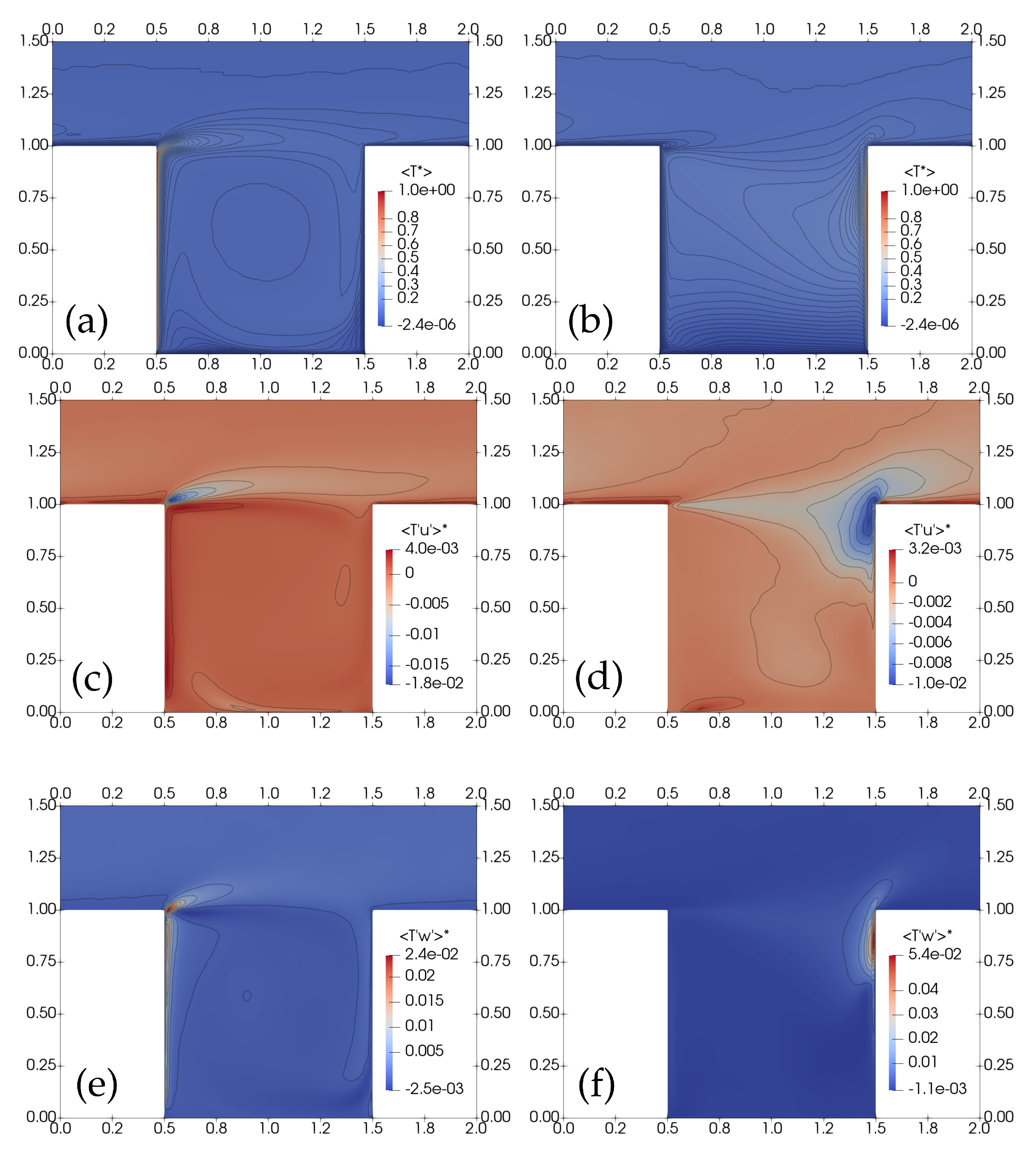
Figure 4a,b displays the temperature distributions for the cases with convection. The favourable case (Figure 4a) shows that temperature is transported from the upwind facade to the interaction and descent-flow regions. The adverse case (Figure 4b) is characterised by a vertical stratification of the canyon. A strong thermal stratification is detectable in the zero-velocity region near the street (see also discussion of Figure 3c), while in the upper-canyon () the high temperature is localised near the downwind facade and weakly transported toward the upwind building by the primary vortex. When the warm air reaches the upwind cold facade, an additional weak vertical convection is generated, leading to an expansion of the left-bottom recirculation region along the facade (see Figure 3c). This contributes to limit the horizontal extent of the main vortex, displacing its centre downwind.
Figure 4c–f presents the vertical and horizontal turbulent thermal fluxes. They can be interpreted through the eddy-viscosity hypothesis (e.g., see Pope [60]):
where is a positive constant, implying that negative (positive) turbulent flux increases (decreases) the temperature diffusion along the direction. Figure 4c,e shows a spot of intense vertical and horizontal fluxes at the left-top corner of the canyon, where the favourable convection deviates the ambient wind. The fluxes increase temperature diffusion in the streamwise direction in the interaction region and downward increasing the vertical mixing. Figure 4d,f displays a zone of high intense fluxes near the top part () of the downwind facade. In this zone, the adverse convection opposes the descent flow driven by the ambient wind. Turbulence diffuses temperature in the streamwise direction also above the building rooftop, and vertically within the canyon against the convective motion.
6.2. First- and Second-Order Statistics over Lines
The effects of favourable and adverse convection are quantitatively analysed comparing the profiles over selected vertical and horizontal lines.
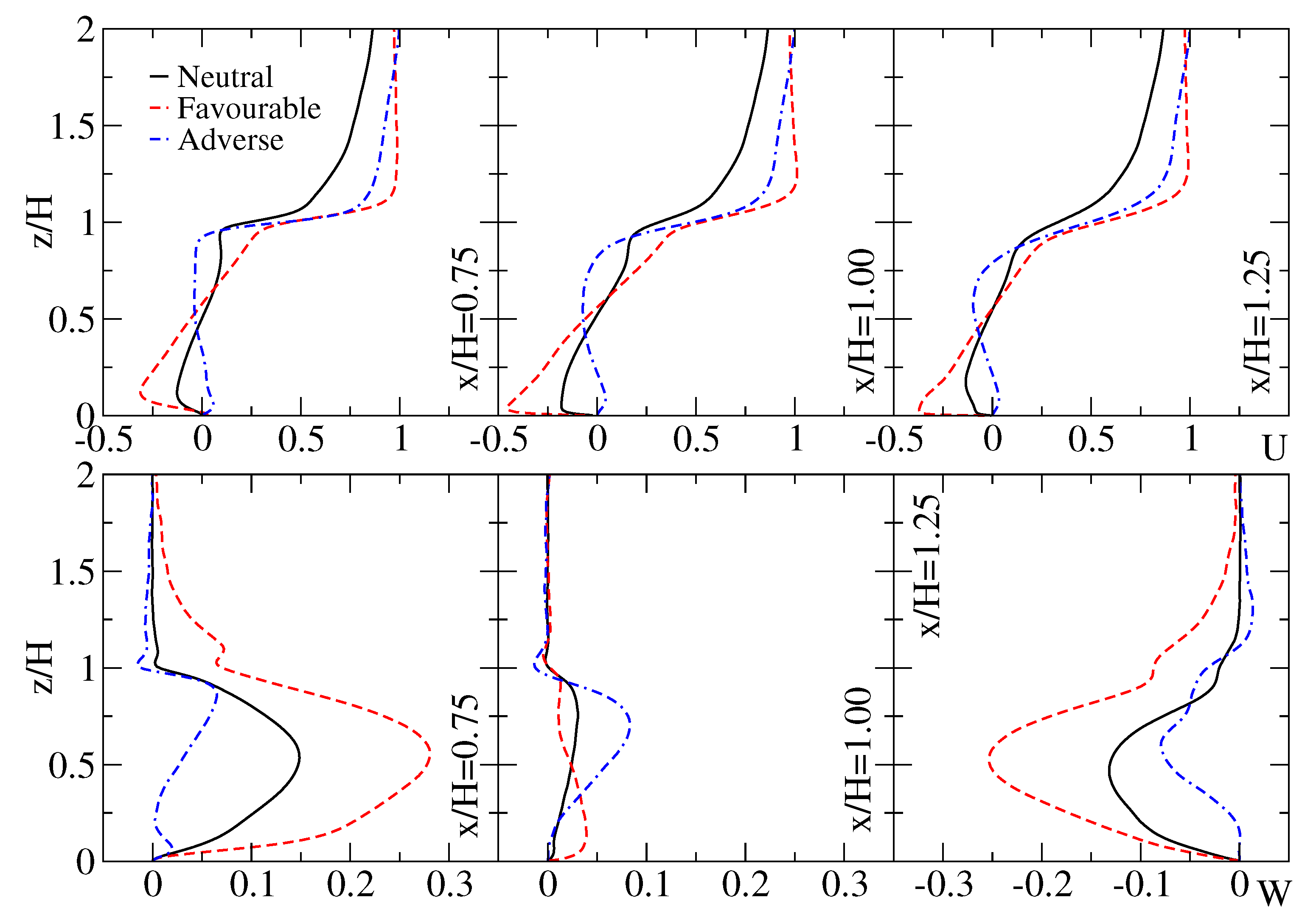
Figure 5 shows the mean non-dimensional vertical and horizontal velocity components along three vertical lines near the upwind building (), at the centerline (), and near the downwind building (). The streamwise velocity (Figure 5 upper panel) reveals that both convective cases produce a higher streamwise velocity above the canyon () compared to the neutral case. The latter shows an almost zero velocity at the rooftop level, and the development of a logarithm-like profile for the ambient wind. Such a behaviour can be ascribed to the strong horizontal shear at the roof level, which acts as a barrier between the canyon and ambient dynamics, mimicking the presence of a solid boundary. This effect is more evident at while it is damped at where the turbulence destabilises the sharp horizontal shear layer. The vertical convection within the canyon destroys the horizontal shear, increasing the turbulent transport of momentum and the mixing at the interface (see Figure 3); hence, the ambient wind velocity is more homogeneously distributed and reaches a constant value above the canyon. The favourable case shows a larger streamwise velocity above the canyon concerning the adverse case because it is more effective in vertical mixing, which is also amplified by the periodicity along the x-direction. Overall, turbulence reduces the drag of the urban canopy and allows more energetic wind velocities. Within the canyon (), the favourable case strengthens the circulation established by the principal vortex, increasing the flow intensity and generating more pronounced horizontal velocity peaks near the street and rooftop levels. On the contrary, the adverse case exhibits a very weak positive velocity in the zero-velocity region, whilst the upper-canyon () is dominated by the (weakened and spatially constrained) principal vortex: negative velocity are detectable in , positive velocity for . The vertical velocity profiles (Figure 5 bottom panel) highlight that in the favourable case the primary vortex velocity is reinforced if compared to the neutral case, and that a weak ascending motion is triggered also above the rooftop (see plot over lines ). The centerline () reports a positive peak in the bottom half of the canyon which is due to the reduction of the bottom-right reticulation region (see Figure 3e). The adverse case displays almost zero velocity in the zero-velocity region and weak values in the upper-canyon coherently with the three-vortex circulation described in Section 6.1. Overall, the profiles of the vertical and horizontal velocity components of the neutral case show intermediate values between the favourable (higher values) and adverse (lower values) cases. This is mainly due to the alteration of the principal vortex, which is enhanced by favourable convection and hampered by adverse convection.
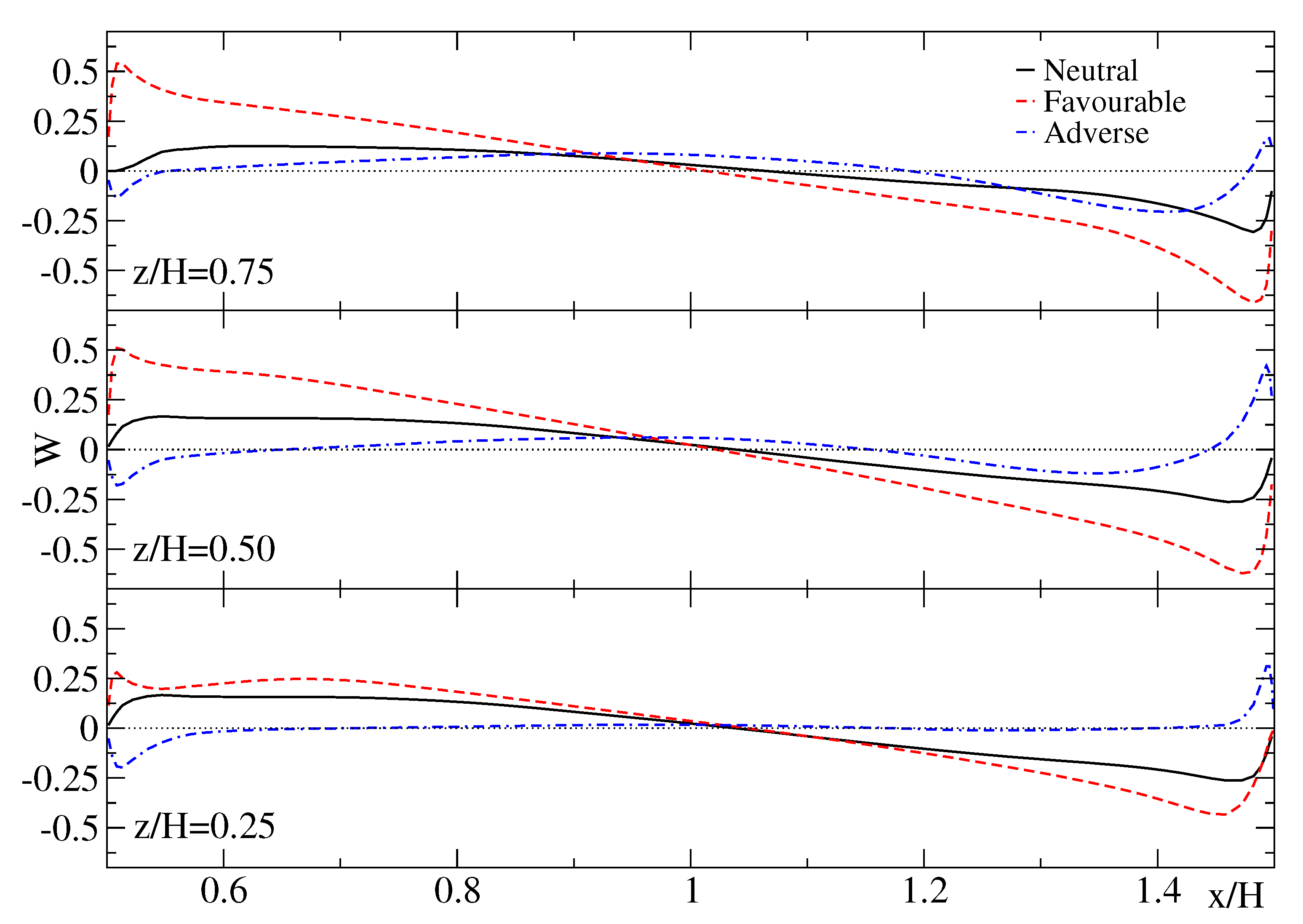
Figure 6 shows the non-dimensional mean vertical velocities along three selected horizontal lines within the canyon. The adverse convection reverses the profiles. Near the downwind facade, the positive velocity is localised in a thin layer near the building surface. The descending flow from the principal vortex has a similar magnitude as in the neutral case at , while becomes weaker at the mid-height and disappears at the lower level . Close to the upwind facade, a peak of weak negative velocity can be generated by the temperature gradient given by the thermal stratification of the canyon.
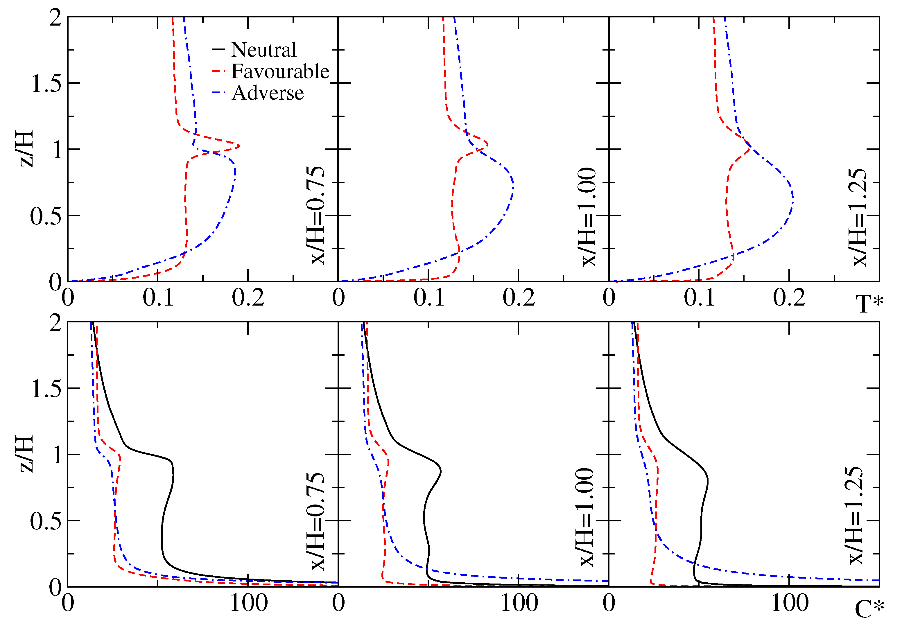
Figure 7 displays the temperature and concentration profiles along three vertical lines. Temperature profiles (top panel) inform that the favourable case is practically not stratified, having an almost constant temperature within and above the canyon. Exceptions are two narrow regions at the street and interface level. The peak of temperature at is due to the transport of temperature by the main canyon vortex, which drives air from the heated facade to the interface region. Instead, the adverse case is strongly stratified in the zero-velocity region and exhibits a moderate vertical temperature gradient in the upper canyon. Outside the canyon, the stratification is almost absent. The overall temperature of the canyon is higher than in the favourable case because the internal air mixing enhances the heat exchange with the hot boundaries. Concentration profiles (bottom panel) shows that convection within the canyon largely improves the pollution removal: both convective cases decrease the concentration levels of the at the canyon mid-high () compare to the neutral case. This is ascribed to the large turbulent mixing triggered by convective motion at the canyon-ambient interface, which improves considerably the exchanges between the canyon and its surroundings. The profiles of the favourable and adverse cases are comparable, but some discrepancies are detectable: the former has a lower level of concentration near the street (lines ) and shows a weak peak at the interface as a consequence of the pollutant transport by the primary vortex. The latter has larger values of concentration in the zero-velocity region, which decreases smoothly with height. Near the upwind facade () the concentration near the street of the favourable case is similar to the adverse case because of the corner recirculation region that entraps part of the pollutant.
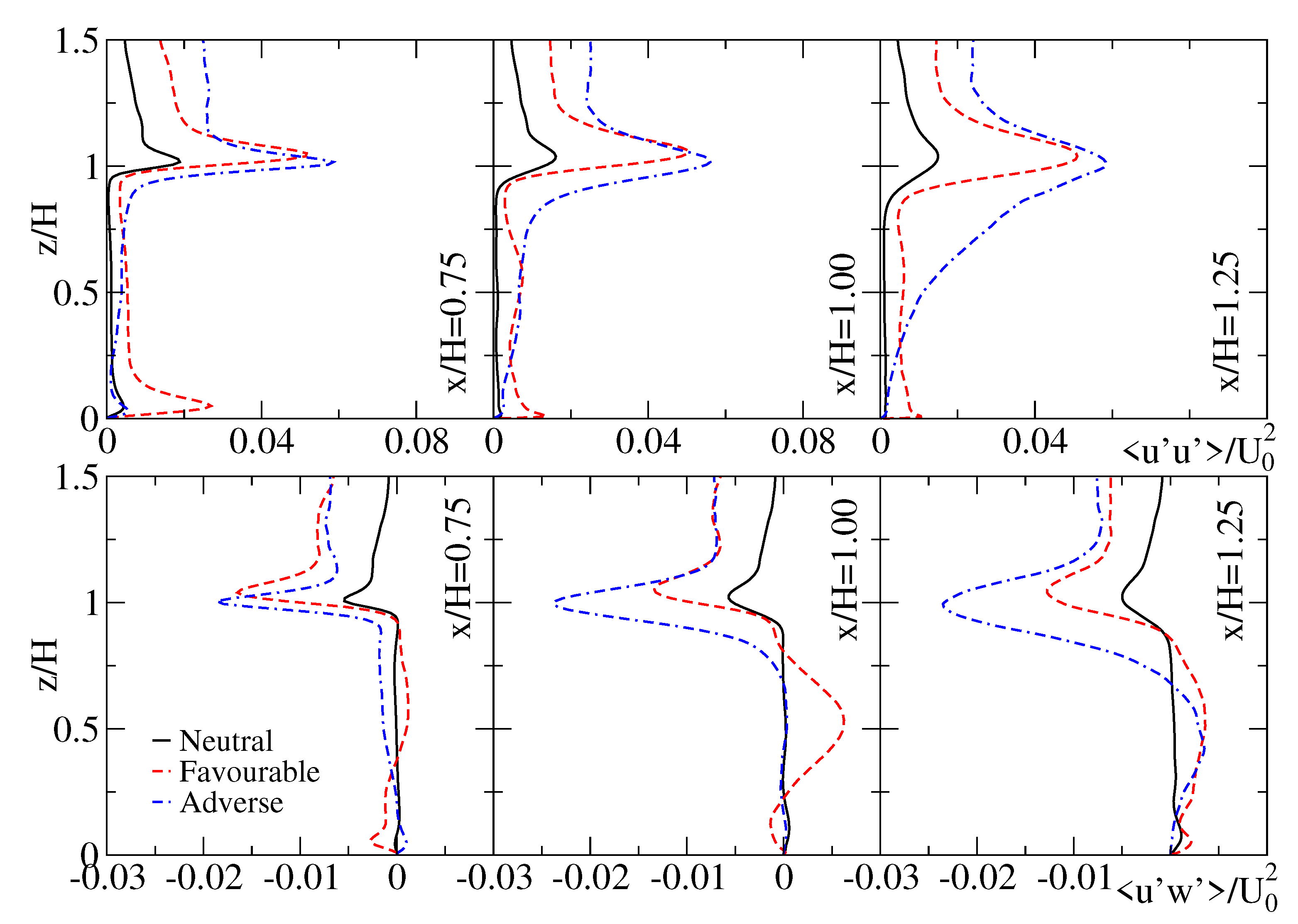
Figure 8 top-panel displays the streamwise fluctuations along three vertical lines. In the neutral case, the fluctuations are almost absent within the canyon, while a local maximum appears at the interface; moderate values characterised the ambient wind. The favourable case shows a similar behaviour but with larger values of streamwise fluctuations: a moderate and constant level of turbulence is detected within the canyon, except near the street level where a local increase is due to the interaction with the recirculation region located in the bottom-left corner (detectable at ). Profiles peak at the interface, as expected. The adverse case exhibits increasing values of fluctuations with the height: in the zero-velocity region are almost zero and smoothly increase until the maximum located at the interface, which is slightly shifted downwards concerning the favourable case. This is caused by the deflection of the interface described in Figure 3. The adverse case displays larger fluctuations in the external region () and a slightly high peak value at the interface. This can be ascribed to the stronger perturbation of the wind flow produced by the adverse convection.
Figure 8 bottom-panel shows the turbulent kinematic momentum fluxes. In neutral case, fluxes are almost zero except at the interface and in a limited area above it. The favourable case has higher values around the canyon centre at line , where inward/outward interdiction events are observed around the low-velocity vortex centre. The positive value within the canyon at line corresponds to the descent-flow region, while the peak of negative fluxes is located at the interface, and non-zero values are detectable in the surrounding ambient flow (see Figure 3). The adverse case reports almost zero fluxes within the canyon, positive values in correspondence with the descent-flow region. The negative peak at the interface is almost twice the value observed in the favourable case at lines , denoting a higher turbulent mixing. The fluxes in ambient flow are similar to the favourable case.
6.3. Additional Thoughts on the Use of a Local Richardson Number
Based on numerical simulations and laboratory experiments reported in the literature, it is noted that a clear definition of Richardson number based only on the quantities characteristic of the canyon region is somehow missing. Although non unequivocally defined, the classical formulation of the Richardson number requires the use of a free-stream velocity and a reference temperature, both computed or measured outside the canopy. On a more theoretical level, we can argue about the effectiveness of these non-dimensional parameters in representing the in-canyon flow regime. Driven respectively by the free-stream velocity and characteristic temperature differences, the inertially- and thermally-driven circulations involve the air volume confined within the canyon. Thus, the definition of a local non-dimensional parameter seems more appropriate although rather complex. In this context, the use of building–building or surface–canyon air temperature differences seem suitable choices: the former addresses the local source of the buoyancy force but it can become of critical computation when the street is also heated; the latter directly infers the buoyancy effect of the canyon air temperature, a fair approximation if the canopy air temperature is isothermal away from the surfaces (e.g., Louka et al. [31]). As for the reference velocity, a characteristic canyon velocity would address the typical flow intensity of the investigated in-canyon circulation. The research of a local parameter can be considered in view of the confined canyon region where the buoyancy force is produced and the effects of the wind force are declined as flow inertia. Examples of local Richardson numbers have been given by Allegrini et al. [26] and Fernando et al. [61]. Both computed a surface-canyon air temperature difference based on an in-canyon air temperature and introduced a characteristic canyon velocity. Allegrini et al. [26] computed the in-canyon quantities in the closest proximity of the heated surface, defining a Richardson number representative of the direct (near-surface) consequences of the buoyancy force exerted by the heated building facade on the canopy flow. Fernando et al. [61] used an inertially-driven canyon velocity determined as the free-stream velocity scaled on the canyon aspect ratio discerned from the continuity equation (see Magnusson et al. [11]). This definition directly addresses the in-canyon effects of the two driving forces.
In this context, the authors propose an alternative formulation for a local Richardson number as follows. The temperature difference involves the characteristic (main) temperature of the upwind building facade and the downwind building facade . Notice that this quantity can be negative. Such a is representative of a configuration where the thermal gradient within the canyon is mealy horizontal, typically observed when the sun heats up a single facade while the opposite one remains in the shadow. Different dynamics arise in presence of vertical thermal gradient, that appears, for example, when the street or the ambient wind has a different temperature with respect to the canyon buildings. In such cases, a vertical thermal gradient tends to impose a stable or unstable temperature stratification within the canyon, with convection from vertical facades being triggered when the hot/cool air is transported near them. Hence, the thermo-dynamics regimes produced by horizontal and vertical temperature gradients are qualitatively different and should be characterised by two different non-dimensional numbers. Since we are interested in vertical interaction between convection and induced flows, the w component along the mid-high horizontal line (thus avoiding boundary effects from the canyon top and bottom) in Figure 6 is scrutinised as characteristic inertial velocity. Specifically, we compute the integral vertical velocity in the left- and right-half canyon as
which are equal thanks to the continuity equation. It is worth noticing that this definition is general and not depending on the particular here considered, by virtue of the principle of Reynolds independence ensured by the case setting (see Section 4.1). As an alternative approximated formulation, can be estimated locally by measuring the maximum and the minimum of the vertical velocity at the mid-high and approximating the integral of the left- and right-half canyon with triangles. The average between the two triangles is a first approximation of the reference velocity: in the present case, this estimation gives .
Using these local formulations of the temperature difference and characteristic canyon velocity, the canyon Richardson number becomes
The has a positive sign if the thermal gradient is directed in the streamwise direction, otherwise, it is negative. Following the setup of this study, a positive indicates a regime of favourable convection, while a negative value indicates adverse convection. The critical values to switch from an inertia-dominated regime to a convection-dominated regime are to be determined separately for the two cases, which is reasonable since the two canyon dynamics are qualitatively different. In the present case, for favourable (positive sign) and adverse (negative sign) convection. It is worth noticing that the definition of here proposed can be further developed to take into account different geometries (e.g., various aspect ratios) and the different heating of the canyon surfaces (e.g., including vertical thermal gradient and surface roughness effects) to better describe the complex configurations that can rise in realistic urban setups.
7. Conclusions
The present contribution analysed and quantified the effects that heated walls in urban canyons have on the flow structures and pollutant removal, which is relevant for practical applications. The large-eddy simulation (LES) approach is adopted to reproduce periodic arrays of infinitely long canyons with unity aspect ratio, where the ambient wind is at and vertical building facades have been set to different temperatures. A flux of pollutant is released at the street level. The dynamic Lagrangian turbulent model by Meneveau et al. [39] has been adopted to reproduce the localised and anisotropic turbulence. Two convective cases have been analysed: the favourable convection case where the upwind facade is heated-up, and the adverse convection case where the downwind facade is heated-up. The Richardson number is set to , being in the range of values measured in real urban canyons. A neutral case with isothermal buildings is also presented as a reference and for validating the numerical approach.
Both the convective cases show an increase in turbulence levels, quantified by the turbulent kinematic momentum and thermal fluxes. The significant increase of turbulence in the interaction region (around the canyon-ambient interface) enhances the vertical mixing and destroys the rooftop horizontal shear layer, increasing the exchange of momentum and mass between the canyon and the surrounding ambient. As a major consequence, the velocity intensity above the canyon exhibits an almost linear profile. Moreover, the pollutant removal from the canyon is largely increased with respect to the neutral case.
In the favourable case, convection strengthens the internal primary clockwise vortex that strongly advects temperature and pollutants along canyon boundaries. The in-canyon pollutant concentration is reduced by compare to the neutral case. In the adverse case, convection counteracts the descending flow of the ambient wind at the downwind facade, strongly reducing the internal circulation. The primary vortex is less energetic and mainly confined in the upper-canyon (). A region of almost zero velocity generates above the street (), having strong thermal stratification and high pollutant concentration values: more than in neutral case and more than in the favourable case. In real settings, this is a critical region since corresponds to the pedestrian level. Also, a thermal stratification arises within the canyon, which further inhibits the internal recirculation. To characterised the different regimes reached by the two convective cases, a definition of a local Richardson number based on in-canyon quantities only (which is lacking in the literature) is proposed.
Author Contributions
Investigation, C.C.; writing—original draft preparation, C.C. and F.B.; supervision and funding acquisition, S.D.S. All authors have read and agreed to the published version of the manuscript.
Funding
This research was funded by the iSCAPE project funded by the European Union’s H2020 Research and Innovation programme (H2020-SC5-04-2015) funded under the Grant agreement No. 689954.
Institutional Review Board Statement
Not applicable.
Informed Consent Statement
Not applicable.
Data Availability Statement
The data can be accessed upon request any of the authors.
Acknowledgments
The authors acknowledge the use of computational resources from the parallel computing cluster of the Open Physics Hub at the Physics and Astronomy Department in Bologna.
Conflicts of Interest
The authors declare no conflict of interest.
References
- Luo, Z.; Li, Y.; Nazaroff, W.W. Intake fraction of nonreactive motor vehicle exhaust in Hong Kong. Atmos. Environ. 2010, 44, 1913–1918. [Google Scholar] [CrossRef]
- Scungio, M.; Stabile, L.; Rizza, V.; Pacitto, A.; Russi, A.; Buonanno, G. Lung cancer risk assessment due to traffic-generated particles exposure in urban street canyons: A numerical modelling approach. Sci. Total. Environ. 2018, 631, 1109–1116. [Google Scholar] [CrossRef] [PubMed]
- Vardoulakis, S.; Fisher, B.E.; Pericleous, K.; Gonzalez-Flesca, N. Modelling air quality in street canyons: A review. Atmos. Environ. 2003, 37, 155–182. [Google Scholar] [CrossRef] [Green Version]
- Buccolieri, R.; Sandberg, M.; Di Sabatino, S. City breathability and its link to pollutant concentration distribution within urban-like geometries. Atmos. Environ. 2010, 44, 1894–1903. [Google Scholar] [CrossRef]
- Buccolieri, R.; Salizzoni, P.; Soulhac, L.; Garbero, V.; Di Sabatino, S. The breathability of compact cities. Urban Clim. 2015, 13, 73–93. [Google Scholar] [CrossRef]
- Chen, L.; Hang, J.; Sandberg, M.; Claesson, L.; Di Sabatino, S.; Wigo, H. The impacts of building height variations and building packing densities on flow adjustment and city breathability in idealized urban models. Build. Environ. 2017, 118, 344–361. [Google Scholar] [CrossRef]
- Barbano, F.; Di Sabatino, S.; Stoll, R.; Pardyjak, E.R. A numerical study of the impact of vegetation on mean and turbulence fields in a European-city neighbourhood. Build. Environ. 2020, 186, 107293. [Google Scholar] [CrossRef]
- Pulvirenti, B.; Baldazzi, S.; Barbano, F.; Brattich, E.; Di Sabatino, S. Numerical simulation of air pollution mitigation by means of photocatalytic coatings in real-world street canyons. Build. Environ. 2020, 186, 107348. [Google Scholar] [CrossRef]
- Dallman, A.; Magnusson, S.; Britter, R.; Norford, L.; Entekhabi, D.; Fernando, H.J. Conditions for thermal circulation in urban street canyons. Build. Environ. 2014, 80, 184–191. [Google Scholar] [CrossRef]
- Cheng, W.C.; Liu, C.H.; Leung, D.Y.C. On the correlation of air and pollutant exchange for street canyons in combined wind-buoyancy-driven flow. Atmos. Environ. 2009, 43, 3682–3690. [Google Scholar] [CrossRef]
- Magnusson, S.; Dallman, A.; Entekhabi, D.; Britter, R.; Fernando, H.J.; Norford, L. On thermally forced flows in urban street canyons. Environ. Fluid Mech. 2014, 14, 1427–1441. [Google Scholar] [CrossRef] [Green Version]
- Chen, G.; Yang, X.; Yang, H.; Hang, J.; Lin, Y.; Wang, X.; Wang, Q.; Liu, Y. The influence of aspect ratios and solar heating on flow and ventilation in 2D street canyons by scaled outdoor experiments. Build. Environ. 2020, 185, 107159. [Google Scholar] [CrossRef]
- Di Sabatino, S.; Barbano, F.; Brattich, E.; Pulvirenti, B. The Multiple-Scale Nature of Urban Heat Island and Its Footprint on Air Quality in Real Urban Environment. Atmosphere 2020, 11, 1186. [Google Scholar] [CrossRef]
- Offerle, B.; Eliasson, I.; Grimmond, C.; Holmer, B. Surface heating in relation to air temperature, wind and turbulence in an urban street canyon. Bound. Layer Meteorol. 2007, 122, 273–292. [Google Scholar] [CrossRef]
- Cai, X.M. Effects of wall heating on flow characteristics in a street canyon. Bound. Layer Meteorol. 2012, 142, 443–467. [Google Scholar] [CrossRef]
- Nazarian, N.; Martilli, A.; Norford, L.; Kleissl, J. Impacts of Realistic Urban Heating. Part II: Air Quality and City Breathability. Bound. Layer Meteorol. 2018, 168, 321–341. [Google Scholar] [CrossRef] [Green Version]
- Barbano, F.; Brattich, E.; Di Sabatino, S. Characteristic scales for turbulent exchange processes in a real urban canopy. Bound. Layer Meteorol. 2021, 178, 119–142. [Google Scholar] [CrossRef]
- Nazarian, N.; Martilli, A.; Kleissl, J. Impacts of Realistic Urban Heating, Part I: Spatial Variability of Mean Flow, Turbulent Exchange and Pollutant Dispersion. Bound. Layer Meteorol. 2017, 166, 367–393. [Google Scholar] [CrossRef]
- Li, X.X.; Britter, R.E.; Norford, L.K.; Koh, T.Y.; Entekhabi, D. Flow and Pollutant Transport in Urban Street Canyons of Different Aspect Ratios with Ground Heating: Large-Eddy Simulation. Bound. Layer Meteorol. 2012, 142, 289–304. [Google Scholar] [CrossRef] [Green Version]
- Nazarian, N.; Kleissl, J. Realistic solar heating in urban areas: Air exchange and street-canyon ventilation. Build. Environ. 2016, 95, 75–93. [Google Scholar] [CrossRef] [Green Version]
- Pulvirenti, B.; Di Sabatino, S. CFD characterization of street canyon heating by solar radiation on building walls. arXiv 2020, arXiv:2006.04800. [Google Scholar]
- Bottillo, S.; Vollaro, A.D.L.; Galli, G.; Vallati, A. Fluid dynamic and heat transfer parameters in an urban canyon. Sol. Energy 2014, 99, 1–10. [Google Scholar] [CrossRef]
- Battista, G.; Mauri, L. Numerical study of buoyant flows in street canyon caused by ground and building heating. Energy Procedia 2016, 101, 1018–1025. [Google Scholar] [CrossRef]
- Gronemeier, T.; Raasch, S.; Ng, E. Effects of Unstable Stratification on Ventilation in Hong Kong. Atmosphere 2017, 8, 168. [Google Scholar] [CrossRef] [Green Version]
- Li, Z.; Zhang, H.; Wen, C.Y.; Yang, A.S.; Juan, Y.H. Effects of height-asymmetric street canyon configurations on outdoor air temperature and air quality. Build. Environ. 2020, 183, 107195. [Google Scholar] [CrossRef]
- Allegrini, J.; Dorer, V.; Defraeye, T.; Carmeliet, J. An adaptive temperature wall function for mixed convective flows at exterior surfaces of buildings in street canyons. Build. Environ. 2012, 49, 55–66. [Google Scholar] [CrossRef]
- Zhao, Y.; Chew, L.W.; Kubilay, A.; Carmeliet, J. Isothermal and non-isothermal flow in street canyons: A review from theoretical, experimental and numerical perspectives. Build. Environ. 2020, 184, 107163. [Google Scholar] [CrossRef]
- Sini, J.F.; Anquetin, S.; Mestayer, P.G. Pollutant dispersion and thermal effects in urban street canyons. Atmos. Environ. 1996, 30, 2659–2677. [Google Scholar] [CrossRef]
- Kim, J.J.; Baik, J.J. Urban street-canyon flows with bottom heating. Atmos. Environ. 2001, 35, 3395–3404. [Google Scholar] [CrossRef]
- Santamouris, M.; Papanikolaou, N.; Koronakis, I.; Livada, I.; Asimakopoulos, D. Thermal and air flow characteristics in a deep pedestrian canyon under hot weather conditions. Atmos. Environ. 1999, 33, 4503–4521. [Google Scholar] [CrossRef]
- Louka, P.; Vachon, G.; Sini, J.F.; Mestayer, P.; Rosant, J.M. Thermal effects on the airflow in a street canyon–Nantes’ 99 experimental results and model simulations. Water Air Soil Pollut. Focus 2002, 2, 351–364. [Google Scholar] [CrossRef]
- Uehara, K.; Murakami, S.; Oikawa, S.; Wakamatsu, S. Wind tunnel experiments on how thermal stratification affects flow in and above urban street canyons. Atmos. Environ. 2000, 34, 1553–1562. [Google Scholar] [CrossRef]
- Kovar-Panskus, A.; Moulinneuf, L.; Savory, E.; Abdelqari, A.; Sini, J.F.; Rosant, J.M.; Robins, A.; Toy, N. A wind tunnel investigation of the influence of solar-induced wall-heating on the flow regime within a simulated urban street canyon. Water Air Soil Pollut. Focus 2002, 2, 555–571. [Google Scholar] [CrossRef]
- Idczak, M.; Mestayer, P.; Rosant, J.M.; Sini, J.F.; Violleau, M. Micrometeorological measurements in a street canyon during the joint ATREUS-PICADA experiment. Bound. Layer Meteorol. 2007, 124, 25–41. [Google Scholar] [CrossRef]
- Xie, X.; Liu, C.H.; Leung, D.Y. Impact of building facades and ground heating on wind flow and pollutant transport in street canyons. Atmos. Environ. 2007, 41, 9030–9049. [Google Scholar] [CrossRef]
- Li, X.X.; Leung, D.Y.C.; Liu, C.H.; Lam, K.M. Physical Modeling of Flow Field inside Urban Street Canyons. J. Appl. Meteorol. Climatol. 2007, 47, 2058–2067. [Google Scholar] [CrossRef]
- Cui, Z.; Cai, X.; Baker, J.C. Large-eddy simulation of turbulent flow in a street canyon. Q. J. R. Meteorol. Soc. 2004, 130, 1373–1394. [Google Scholar] [CrossRef]
- Rodi, W.; Constantinescu, G.; Stoesser, T. Large-Eddy Simulation in Hydraulics, 3rd ed.; CRC Press, Taylor and Francis Group: Boca Raton, FL, USA, 2013. [Google Scholar]
- Meneveau, C.; Lund, T.; Cabot, W. A Lagrangian dynamic subgrid-scale model of turbulence. J. Fluid Mech. 1996, 316, 353. [Google Scholar] [CrossRef] [Green Version]
- Cintolesi, C.; Pulvirenti, B.; Di Sabatino, S. Large-Eddy Simulations of Pollutant Removal Enhancement from Urban Canyons. Bound. Layer Meteorol. 2021. [Google Scholar] [CrossRef]
- Van Driest, E. On turbulent flow near a wall. J. Aeronaut. Sci. 1956, 23, 1007–1011. [Google Scholar] [CrossRef]
- Cintolesi, C.; Petronio, A.; Armenio, V. Large eddy simulation of turbulent buoyant flow in a confined cavity with conjugate heat transfer. Phys. Fluids 2015, 27. [Google Scholar] [CrossRef] [Green Version]
- Cintolesi, C.; Petronio, A.; Armenio, V. Large-eddy simulation of thin film evaporation and condensation from a hot plate in enclosure: First order statistics. Int. J. Heat Mass Transf. 2016, 101, 1123. [Google Scholar] [CrossRef] [Green Version]
- OpenFOAM. The OpenFOAM Foundation. 2018. Version 6.0. Available online: openfoam.org (accessed on 1 May 2019).
- Cintolesi, C.; Petronio, A.; Armenio, V. Turbulent structures of buoyant jet in cross-flow studied through large-eddy simulation. Environ. Fluid Mech. 2019, 19, 401–433. [Google Scholar] [CrossRef] [Green Version]
- Jasak, H.; Weller, H.; Gosman, A. High resolution NVD differencing scheme for arbitrarily unstructured meshes. Int. J. Numer. Meth. Fluids 1999, 31, 431–449. [Google Scholar] [CrossRef]
- Michioka, T.; Sato, A.; Takimoto, H.; Kanda, M. Large-Eddy Simulation for the Mechanism of Pollutant Removal from a Two-Dimensional Street Canyon. Bound. Layer Meteorol. 2011, 138, 195–213. [Google Scholar] [CrossRef]
- Chew, L.; Aliabadi, A.; Norford, L. Flows across high aspect ratio street canyons: Reynolds number independence revisited. Environ. Fluid Mech. 2018, 18, 1275–1291. [Google Scholar] [CrossRef]
- Nakamura, Y.; Oke, T.R. Wind, temperature and stability conditions in an east-west oriented urban canyon. Atmos. Environ. 1988, 22, 2691–2700. [Google Scholar] [CrossRef]
- Aliabadi, A.; Moradi, M.; Clement, D.; Lubitz, W.; Gharabaghi, B. Flow and temperature dynamics in an urban canyon under a comprehensive set of wind directions, wind speeds, and thermal stability conditions. Environ. Fluid Mech. 2019, 19, 81–109. [Google Scholar] [CrossRef]
- Piomelli, U.; Balaras, E. Wall-Layer Models for Large-Eddy Simulations. Annu. Rev. Fluid Mech. 2002, 34, 349–374. [Google Scholar] [CrossRef] [Green Version]
- Trivellato, F.; Raciti Castelli, M. On the Courant–Friedrichs–Lewy criterion of rotating grids in 2D vertical-axis wind turbine analysis. Renew. Energy 2014, 62, 53–62. [Google Scholar] [CrossRef]
- Brown, M.J.; Lawson, R.E.; Decroix, D.S.; Lee, R.L. Mean Flow and Turbulence Measurement around a 2-D Array of Buildings in a Wind Tunnel. In Proceedings of the AMS 11th Joint Conference on The Applications of Air Pollution Meteorology, Long Beach, CA, USA, 9–14 January 2000; Report LA-UR-99-5395. [Google Scholar]
- Germano, M. Turbulence: The filtering approach. J. Fluid Mech. 1992, 238, 325. [Google Scholar] [CrossRef]
- Lilly, D. A proposed modification of Germano subgrid-scale closure method. Phys. Fluids 1992, A4, 633. [Google Scholar] [CrossRef]
- Meroney, R.N.; Pavageau, M.; Rafailidis, S.; Schatzmann, M. Study of line source characteristics for 2-D physical modelling of pollutant dispersion in street canyons. J. Wind. Eng. Ind. Aerodyn. 1996, 62, 37–56. [Google Scholar] [CrossRef]
- Pavageau, M.; Schatzmann, M. Wind tunnel measurements of concentration fluctuations in an urban street canyon. Atmos. Environ. 1999, 33, 3961–3971. [Google Scholar] [CrossRef]
- Göthe, C.J.; Bjurström, R.; Ancker, K. A Simple Method of Estimating Air Recirculation in Ventilation Systems. Am. Ind. Hyg. Assoc. J. 1988, 49, 66–69. [Google Scholar] [CrossRef]
- Buccolieri, R.; Gromke, C.; Di Sabatino, S.; Ruck, B. Aerodynamic effects of trees on pollutant concentration in street canyons. Sci. Total. Environ. 2009, 407, 5247–5256. [Google Scholar] [CrossRef] [PubMed]
- Pope, S. Turbulent Flows; Cambridge University Press: Cambridge, UK, 2000. [Google Scholar]
- Fernando, H.J.; Zajic, D.; Di Sabatino, S.; Dimitrova, R.; Hedquist, B.; Dallman, A. Flow, turbulence, and pollutant dispersion in urban atmospheres. Phys. Fluids 2010, 22, 051301. [Google Scholar] [CrossRef]
Figure 1.
Sketch of the simplified urban canyon geometry and computational mesh used. (a) The geometry of the case study. The computational domain is bounded by dashed lines; the red line in the canyon delimits the pollutant release region. (b) Overview of the computational mesh.
Figure 1.
Sketch of the simplified urban canyon geometry and computational mesh used. (a) The geometry of the case study. The computational domain is bounded by dashed lines; the red line in the canyon delimits the pollutant release region. (b) Overview of the computational mesh.

Figure 2.
Non-dimensional mean streamwise velocity u, its root-mean square , the turbulent kinematic momentum flux and the concentration . Quantities are plotted along the canyon centre line . Lines are numerical simulations: black solid line, present LES of neutral case (); pink dashed line, LES by Michioka et al. [47]. Symbols are laboratory measurements: black ∘, Li et al. [36]; red □, Brown et al. [53]; light green ⋄, experiment Michioka et al. [47]; blue +, Chew et al. [48]; dark green △, Meroney et al. [56]; violet *, Pavageau and Schatzmann [57].

Figure 3.
Velocity streamlines, concentration and turbulent kinematic momentum flux contour lines at a vertical plane perpendicular to the canyon () for the thee cases under consideration: first column, neutral case; second column, favourable case; third column, adverse case. The colour background shows the spatial distribution of quantities, which are made non-dimensional and averaged. (a–c) The non-dimensional mean velocity magnitude . (d–f) The non-dimensional mean concentration . (g–i) The non-dimensional mean turbulent kinematic momentum flux .

Figure 4.
Non-dimensional mean temperature, streamwise and vertical thermal fluxes distribution at a vertical plane perpendicular to the canyon () for the thee cases under consideration: first column, favourable case; second column, adverse case. (a,b) Temperature. (c,d) Horizontal thermal fluxes ). (e,f) Vertical thermal fluxes ).

Figure 5.
Non-dimensional mean velocity components, and , along three selected vertical lines .

Figure 6.
Non-dimensional mean vertical velocity, , along three selected horizontal lines .

Figure 7.
Non-dimensional mean temperature and concentration along three selected vertical lines .

Figure 8.
Resolved Reynolds stress component in streamwise direction and turbulent kinematic momentum fluxes , averaged and made non-dimensional through . Profiles along three selected vertical lines .
Figure 8.
Resolved Reynolds stress component in streamwise direction and turbulent kinematic momentum fluxes , averaged and made non-dimensional through . Profiles along three selected vertical lines .


Table 1.
Non-dimensional numbers that characterised the case study and thermo-dynamic parameters of the working fluid (air).
Table 1.
Non-dimensional numbers that characterised the case study and thermo-dynamic parameters of the working fluid (air).
| Parameter | |||
|---|---|---|---|
| Reynolds | Re | ... | |
| Grashof | Gr | ... | |
| Richardson | Ri | ... | |
| Prandlt | Pr | ... | |
| Schmidt | Sc | ... | |
| Free-stream velocity | m/s | ||
| Temperature difference | K | ||
| Gravity acceleration | g | m/s | |
| Kinematic viscosity | m/s | ||
| Thermal conductivity | m/s | ||
| Concentration conductivity | m/s | ||
| Expansion coefficient | 1/K |
Table 2.
Typical values of several thermo-dynamic quantities and parameters from field investigations. The dash highlights the values range, while values on different lines for are separately investigated in the reference study.
Table 2.
Typical values of several thermo-dynamic quantities and parameters from field investigations. The dash highlights the values range, while values on different lines for are separately investigated in the reference study.
| Field Study | H [m] | H/W | [m/s] | ∣∣ [K] | Re (×10) | Gr (×10) | Ri |
|---|---|---|---|---|---|---|---|
| Nakamura and Oke [49], | 17 | 1.06 | 0.71–1.71 | 2–14 | 0.81–1.93 | 0.68–2.05 | 0.28–3.19 |
| Kyoto (JP) | |||||||
| Santamouris et al. [30], | 21 | 2.47 | 1.00–4.00 | 0.5–13 | 1.40–5.60 | 1.00–25.6 | 0.81–13.04 |
| Athens (GR) | |||||||
| Louka et al. [31], | 21.1 | 1.40 | 1.00 | 0–18 | 1.41 | 0–25.5 | 0–12.83 |
| Nantes (FR) | |||||||
| Offerle et al. [14], | 15 | 2.10 | 0.84–1.86 | ≥1 | 0.84–1.86 | ≤0.35 | ≤0.10 |
| Gothenburg (SE) | ≤16 | ≥0.71 | ≥1.00 | ||||
| Aliabadi et al. [50], | 13 | 1.00 | 1.00 | 0–10 | 1.00 | 0–0.10 | 0–0.10 |
| Guelph (CA) | |||||||
| Di Sabatino et al. [13], | 33 | 1.67 | 0.65–2.50 | 1–10 | 1.43–5.94 | 10.9–18.1 | 0.61–6.34 |
| Bologna (IT) | |||||||
| Controlled field study | ... | ... | ... | ... | Re (×10) | Gr (×10) | ... |
| Idczak et al. [34], | 5.2 | 2.48 | ≤2.00 | 0.5–9 | ≤6.93 | 0.05–2.40 | 0.01–0.50 |
| Guerville (FR) | |||||||
| Chen et al. [12], | 1.2 | 1/3 | 0.10–2.00 | 10 | 0.08–1.64 | 2.65–2.70 | 0.10–39.2 |
| Guangzhou (CN) |
Table 3.
Non-dimensional concentration density and the main recirculation quotient within three selected regions: the entire domain (), the canyon region (), and the zero-velocity region (). Percentage are computed with respect to the entire domain concentration.
Table 3.
Non-dimensional concentration density and the main recirculation quotient within three selected regions: the entire domain (), the canyon region (), and the zero-velocity region (). Percentage are computed with respect to the entire domain concentration.
| Entire Domain | Canyon Region | Zero-Velocity Region | ||
|---|---|---|---|---|
| Neutral case | 24.05 | 55.88 | 69.14 | |
| 1.00 | 0.46 | 0.11 | ||
| Favourable case | 18.52 | 28.77 | 36.50 | |
| 1.00 | 0.31 | 0.08 | ||
| Adverse case | 18.79 | 40.67 | 96.627 | |
| 1.00 | 0.43 | 0.20 |
Publisher’s Note: MDPI stays neutral with regard to jurisdictional claims in published maps and institutional affiliations. |
© 2021 by the authors. Licensee MDPI, Basel, Switzerland. This article is an open access article distributed under the terms and conditions of the Creative Commons Attribution (CC BY) license (https://creativecommons.org/licenses/by/4.0/).
Share and Cite
MDPI and ACS Style
Cintolesi, C.; Barbano, F.; Di Sabatino, S. Large-Eddy Simulation Analyses of Heated Urban Canyon Facades. Energies 2021, 14, 3078. https://doi.org/10.3390/en14113078
AMA Style
Cintolesi C, Barbano F, Di Sabatino S. Large-Eddy Simulation Analyses of Heated Urban Canyon Facades. Energies. 2021; 14(11):3078. https://doi.org/10.3390/en14113078
Chicago/Turabian StyleCintolesi, Carlo, Francesco Barbano, and Silvana Di Sabatino. 2021. "Large-Eddy Simulation Analyses of Heated Urban Canyon Facades" Energies 14, no. 11: 3078. https://doi.org/10.3390/en14113078
Note that from the first issue of 2016, this journal uses article numbers instead of page numbers. See further details here.