Modelling Morphological Changes and Migration of Large Sand Waves in a Very Energetic Tidal Environment: Banks Strait, Australia

Abstract

Banks Strait, Tasmania, Australia, has been identified as a potential site for the deployment of tidal turbines. In this study, the characterization of sediment transport and large sand waves for this site is performed. Observations of bed level change collected from surveys in 2018 showed a migration of large sand waves over a period of nine months. Migration rates in an excess of one hundred meters for nine months were found, which are large compared to the rate reported at other coastal sites, by several meters per year. A validated hydrodynamic model is coupled with a morphodynamic model to perform sensitivity tests and identify what parameters influence migration to better understand sediment dynamic in the Banks Strait. Numerical analysis showed a constant shift of the sand waves profile in an eastward direction, consistent with the observations. This migration was strongly linked with tidal asymmetry, with a residual current flowing towards the east. The principal parameters driving the migration of sand waves in the Banks Strait were found to be sediment sorting, bed friction and residual current. This study gives new insights for the seabed of Banks Strait and provides an assessment of the natural variability of sediment for futures tidal farms deployments.

1. Introduction

Increasing activity in ocean renewables and blue economy is driving the need to understand natural sediment processes and their variability and also to understand the potential influence of anthropogenic activities on them. In coastal environments, sediment plays an important role in the functioning and structuring of coastal ecosystems and is a crucial component for tidal site assessment [1,2]. In shallow straits with sandy bed formations, tidal motion influences the bedform, and rhythmic, large-scale bedforms are commonly present. Tidal sand waves are the most dynamic bedform and very large sand waves were found recently in the Banks Strait, a promising site for future deployment of tidal farm, connecting the Bass Strait to the Tasman Sea (Figure 1). Such large sand waves of more than five meters heights and wavelengths of more than 100 m have also been found in other areas, such as the Taiwan banks, San Francisco bay, North Sea, and in more energetic sites, such as the Torres Strait (Australia), in the Alderney Race (English channel) and are listed alongside other observed sand waves in

Table 1. Characteristics of sand waves from observations.

Environment	Source	Location	Wave Length (m)	Wave Height (m)	Migration Rate (m/Year)	Max Tidal Velocity (m/s)
Coastal regions	Besio [4]	North Sea	120–500	2–10	1–8	/
Coastal regions	Tonnon [5]	North Sea	250–370	1.3–4	average: 5.5	/
Coastal regions	Van Dijck [6]	North Sea	100–800	1–10	0–40	/
Coastal regions	Knaapen [7]	North Sea	110–340	0.7–3.4	0–8.4	/
Coastal regions	Roos [8]	Southern North Sea	145–760	1.5–7.3	/	/
Coastal regions	Bellec [9]	Western Barrents Sea	300–700	4–19	/	1
Coastal regions	Hoozemans [10]	Dutch Sea	/	/	up to 200	/
Strait	Daniell [11]	Torres Strait (AUS)	∼62	5–10	15–48 m over 7 month	2
Strait	Katoh [12]	Bisanseto Sea (JAP)	80–180	2–6	up to 20	/
Strait	Malikides [13]	Bass strait (AUS)	55–1730	2–12	/	1
Strait	Zhou [14]	Taiwan Banks	100–2000	1.5–15	1–5	1
Strait	Blunden [15]	Alderney Race (UK–FR)	/	5–10	0–70 m for 50days	/
Strait (not shallow)	Santoro [16]	Messina strait (ITA)	50–150	0.5–6	/	1.5
Bay	Barnard [17]	San Francisco (USA)	30–220	4–10	7	2–2.5
Tidal Bay	Dalrymple [18]	Bay of Fundy (CAN)	10–215	0.15–3.4	/	0.5–2
Tidal inlet	Buijsman [19]	North Sea	125–250	1–7	0–90	/
Tidal inlet	Bartholdy [20]	Danish Wadden Sea	50–250	1.3–3.6	average: 32	1.5–1.25

. Sediment dynamics and migration of sand waves alter the profile of the seabed and may pose risks to the tidal energy industry, exposing cables and affecting the stability of offshore structures. It is essential to investigate the mechanisms responsible for sediment dynamics, as part of a global environmental impact assessment of large arrays installations, to better understand the influence induced by human activities. Moreover, regulators want to know how tidal farms might affect the marine environment, thus an assessment of the natural variability of the sediments must be carried out at prospective sites. Given the scarcity of in situ data, improving our understanding of the complex processes of sediment transport and sand waves migrations is one of the challenges in high energetic sites.

Few studies on sediment dynamics and seabed characterisation exist for the south of Bass Strait. Only earlier studies, mostly conducted in the 1980–1990s, are available [3,13,21,22,23,24,25,26,27]. More recently, two surveys by Geoscience Australia (GA) took place in this area (GA 226/233) [28,29]. Of these studies, only one study has focused on the Banks Strait [3], which describes the geology of this channel as cold-water carbonates, and is a valuable source of sediment grabs information in this region (Figure 1). Information on the Banks Strait can be found from larger studies of the Bass strait, such as [24] who proposed a map of the sediment types for Bass Strait, including the Banks Strait, with results in accordance with the observations of [29], who indicates for Banks Strait a mean grain size between 0.5 and 2 mm (coarse sand). Sand waves in the Banks strait area were first reported by Slater in 1969 [3] (Figure 1) and then by Malikides in 1988 [13] based on the work of [3] but were not studied. During these studies, only sand waves around Flinders Island were investigated with sediment sampling and side-scan sonar [13,23]. Since then, no other seafloor features of Banks Strait has been investigated, due to limited data and harsh conditions in this energetic site.

Observations and numerical modelling are the keys to understanding the sediment and sand wave dynamics. However, full-scale bathymetry survey are often limited, as surveys are expensive and challenging in highly energetic sites with current speeds above 2 m/s. The initial formation of sand waves has been extensively studied with linear and nonlinear stability analysis [4,30,31,32,33,34,35,36]. From these studies, the migration of sand waves was found to occur as the result of the residual current and tide asymmetry. More recently, more complex numerical shallow models were used to investigate the formation, migration and also the effect of parameters (tidal forcing, significant wave height, turbulence scheme, sediment size) on the evolution of sand waves: Tonnon [5] with the study of artificial sand waves, Borsje [37] who studied two turbulence models associated with bed load transport only, Van Gerwen [38] who focussed on formation of sand waves with comparable migration patterns to observations, and Wang [39] who examined the sensitivity of sand waves to environmental factors. All of them found that the variation of the shape and evolution of the sand waves was linked to sediment grain sizes, tidal characteristics, and residual currents. So far, all of these studies considered medium sand in less energetic areas than the Banks Strait and did not include models with waves. According to King [40] and Fairley [41], waves could heavily influence sediment dynamic in energetic tidal environments. The presence of waves increases turbulence at the seabed, leading to an increase in the bed shear stress and therefore, a greater potential for sediment movement. In the Banks Strait, significant wave–tide interactions were found by [42,43]; thus, it is crucial to consider wave forcing for the sand transport in this tidal energetic site.

In this study, sediment observations and a high resolution sand transport model coupled with the hydrodynamic model with waves forcing (the shallow water model MIKE 21FM [44]) were combined to model and, therefore, enhance our knowledge of the sediment transport processes and the mechanisms driving the migration of sand waves in the Banks Strait. Numerical sensitivity experiments were performed to investigate the response of sand waves to environmental parameters and compared with the survey data set (including data from multi-beam surveys and sub bottom profiling). Parameters driving most of the sand wave morphology were identified in this high energetic site and compared with the literature. Section 2 presents the description of the model with the set up of hydrodynamics, sediment parameters and the surveys performed in 2018, followed by the validation of the hydrodynamic model. Finally the results for the sensitivity analysis are presented and discussed in Section 3, and the conclusion in Section 4.

2. Morphological Set Up

This section first describes the surveys performed by the AUSTEn project in the Banks Strait, whose main goal was to assess Australia’s tidal energy resource through several field surveys to highlight the opportunities available for the emerging tidal industry, the scientific community and the Australian Renewable Energy Agency (ARENA) [45]. Second, the model set-up for the hydrodynamics and sediment transport processes are presented as well as the method for the sand waves analysis. Then, the validation of the hydrodynamic model against in situ data from Acoustic Doppler Current Profilers (ADCP) deployed during the campaigns is described.

2.1. Survey of Banks Strait

The Banks Strait is a shallow channel located in the north east of Tasmania between Cape Portland and Clarke Island, with the tidal constituent $M_2$ as the dominant. Multiple data sets, including hydrodynamic (current speed, waves) and sediment data, were collected by the AUSTEn project [45] to develop and model the Banks Strait area during four campaigns: March, July and December 2018 and February 2019 [43,46,47,48]. During this period, significant wave height (Hs) were measured and varied between 1 and 2 m (maximum up to 5 m) with wave period between 7 and 12 s [48]. High current speed (>2 m/s) suitable for implementation of tidal farm were found near the area of the sand waves which were also found by numerical modelling of the area [43,47,49]. It should be noted that two ADCP frames were buried under at least 1 m of sand at the location of sand waves and could not be retrieved. Seabed characterisation performed during the AUSTEn project included the following: multi-beam transects to collect accurate bathymetry of the site; sub-bottom profiling for high-resolution imaging of sub-seabed sediments; penetrometer casts to describe the hardness of surficial seafloor sediments as well as the collection of sediment samples to determine sediment size and type with bottom grabs and sediment traps.

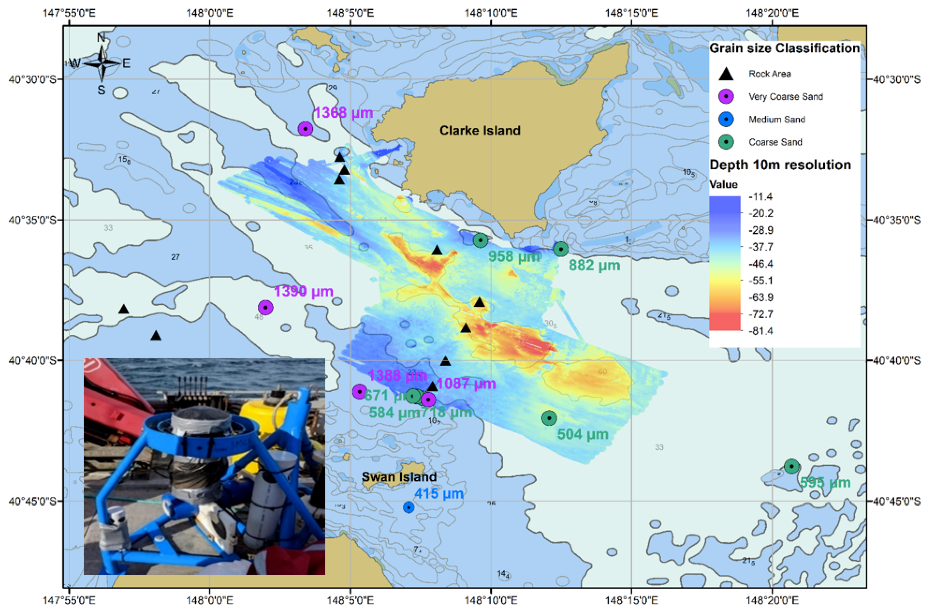
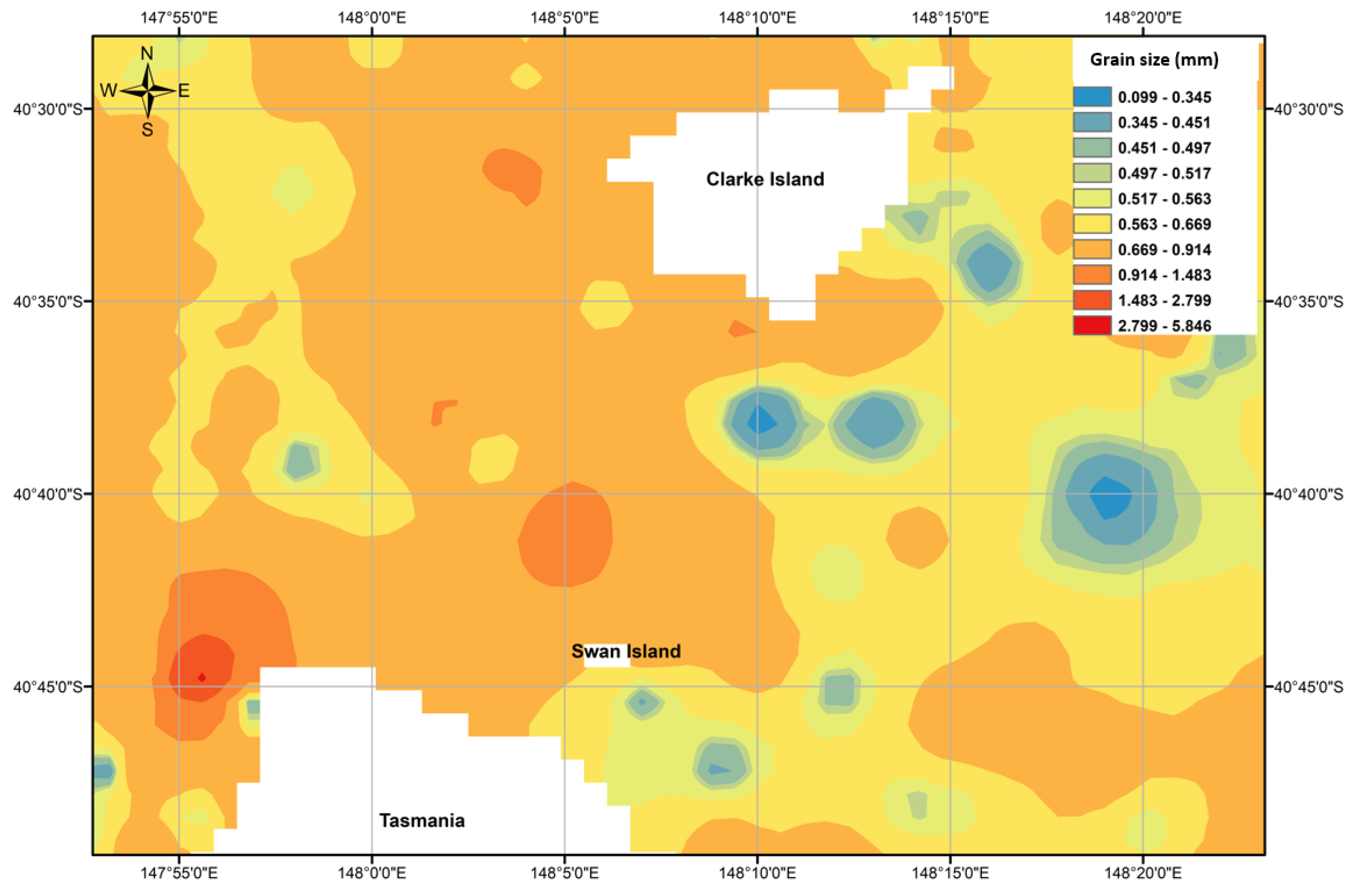
2.1.1. Multi-Beam/Bottom Grab/Sediment Traps

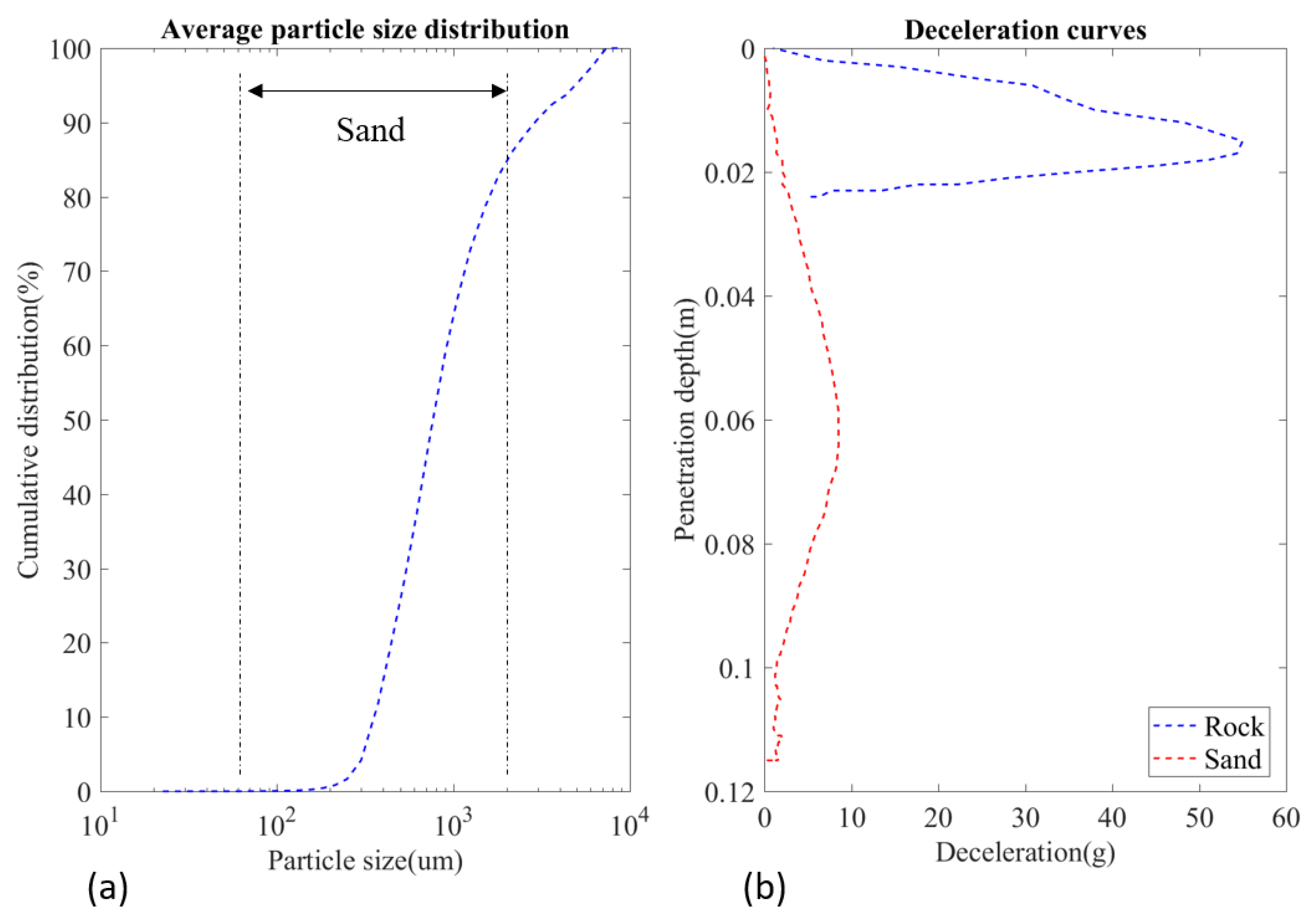
Bathymetry was measured with the Bathyswath interferometric bathymetry system (234 kHz unit from ITER Systems). The bathymetry survey covered an area of approximately 210 km${}^2$ with depths ranging from 10 m to depths exceeding 90 m (Figure 2). To complete the sediment data set, bottom grabs and sediment trap samplings were performed using a Van Veen Grab sampler [50] and sediment sampling traps (

Table A1. Bottom Grab (G) and Sediment Traps (ST) characteristics.

	Latitude	Longitude	Date	Mean Grain Size	Wentworth [51] Classification
G1/ ST_C1	−40.6727	148.2388	6 December 2019–16 February 2019	671 µm	CS
G2	−40.69005	148.1296	8 December 2018	1087 µm	VCS
G6	−40.6354	148.0332	10 December 2018	1390 µm	VCS
G9	−40.59549	148.1606	10 December 2018	958 µm	CS
G10	−40.60083	148.2083	10 December 2018	882 µm	CS
G11	−40.68528	148.089	10 December 2018	1388 µm	VCS
G12	−40.75377	148.118	10 December 2018	415 µm	MS
ST_CW2	−40.701	148.2013	12 July 2018–7 December 2018	504 µm	CS
ST_CW4	−40.7296	148.345	13 July 2018–7 December 2018	595 µm	CS
ST_CW1	−40.5294	148.0568	12 July 2018–12 December 2018	1368 µm	VCS
ST_Swan1	−40.68815	148.1228	6 December 2019–16 February 2019	584 µm	CS
ST_Swan2	−40.68788	148.1205	6 December 2018–8 December 2018	718 µm	CS

in Appendix A). Twelve bottom grabs were conducted during the December campaign: eight were successful, and four were rejected from analysis, given that the grabs trapped nothing indicating a rocky area. Sediments traps were put on six ADCP frames during the campaign in July and December 2018 and retrieved in December 2018 and February 2019 (Figure 2). All sediment samples were emptied into a plastic container after retrieval and stored in a refrigerator. For the grain size analysis, 100 g to 200 g of each sample were oven dried at 60 degrees Celsius for 24 h. The samples were analysed using a Sympatec QICPIC particle size analyser.

The Wentworth scale [51] was used to classify the sediment size from the mean diameter with the results shown on Figure 2. The sediment size for twelve locations were obtained; for different samples at the same location, the mean of grain size was taken (

Table A2. Bottom Grab (G) and Sediment Traps (ST) characteristics with Folk diagram modified from [53].

	Mud%	Sand%	Gravel%	Sediment Type
G1/ST_C1	/	85	14	gravelly Sand
G2	/	89	11	gravelly Sand
G6	/	59	41	sandy Gravel
G9	/	88	12	gravelly Sand
G10	/	88	12	gravelly Sand
G11	/	68	32	sandy Gravel
G12	/	100	0.2	Sand
ST_CW2	/	98	2	slighty gravelly Sand
ST_CW4	/	97	3	slighty gravelly Sand
ST_CW1	/	67	33	sandy Gravel
ST_Swan1	/	96	4	slighty gravelly Sand
ST_Swan2	/	88	12	gravelly Sand

in Appendix A). Sand was a dominant fraction in all samples, consisting mainly of coarse and very coarse sand (Figure 3a). The only exceptions were samples at the south of Swan Island where medium sand was found. The results for the sorting following the classification of [52] revealed that one sample consisted of well sorted (near Swan Island), eight moderately sorted and three poorly sorted sediment (concentrated in the middle of the strait). Mixed sediment was classified according to the modified Folk diagram [53], which relates the proportions of mud, sand and gravel by the ratio of sand to mud and the percentage of gravel (

Table A3. Bottom Grab (G) from the 2018 AUSTEn survey compared to the 1966 survey performed by R.Slater [3].

	2018	1966
G6	sandy Gravel	gravelly Sand
G11	sandy Gravel	sandy Gravel
G12	Sand	Sand

in Appendix A). This analysis confirmed sand was the dominant fraction. Data from a previous seabed survey in Banks Strait [3] were used for comparison. The comparison of three samples showed the same classification, except for grab 6 (West of the Banks Strait), where it was slightly different: sandy gravel in 2018 and gravelly sand in 1966 [54]. This can be explained by the lower quantity collected for this sample (20,000 particles analysed against a mean of 325,000 for the two other samples), which does not cover the whole spectrum of sediment in this location.

2.1.2. Penetrometer

In situ measurements of surficial seafloor sediment strength was determined with the BlueDrop penetrometer described by [55,56]. The characteristics of the impact signature were analysed to obtain the kind of substrate—soft, medium, and hard substrate—based on the deceleration curves after impact. Hard substrate is indicated by the deceleration to zero velocity in a shorter period of time, than into a soft ground (Figure 3b). Each penetrometer drop included three casts from which the mean penetration depth (distance between free fall and complete stop after impact with seafloor) was taken. The majority of penetration depths range between 0.01 and 0.04 m, which is typical for bedrock dominated area. Five drops had penetration depths superior to 0.1 m characteristic of sandy area and were located South of the Clarke Island, towards Swan Island and at the east of the channel.

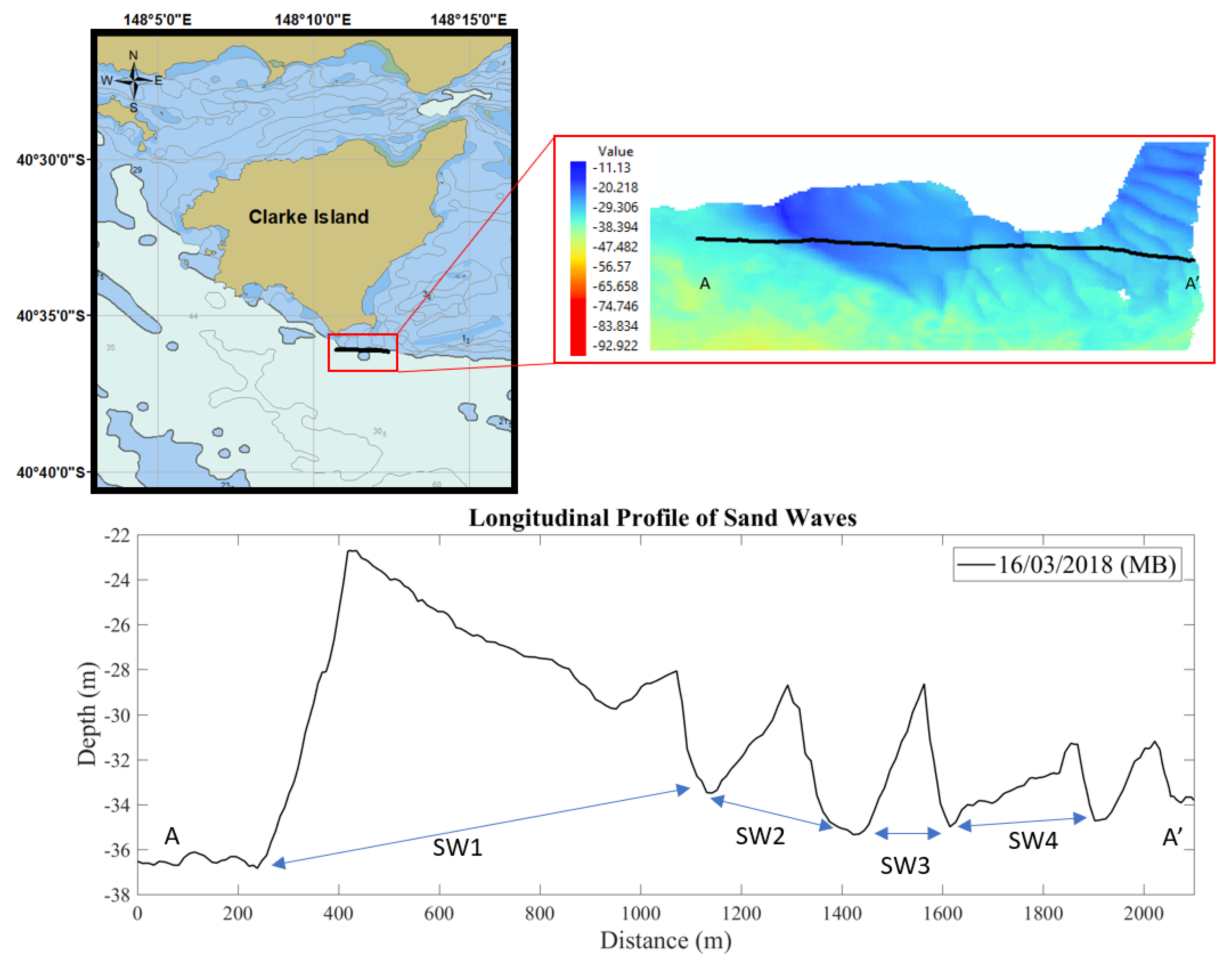
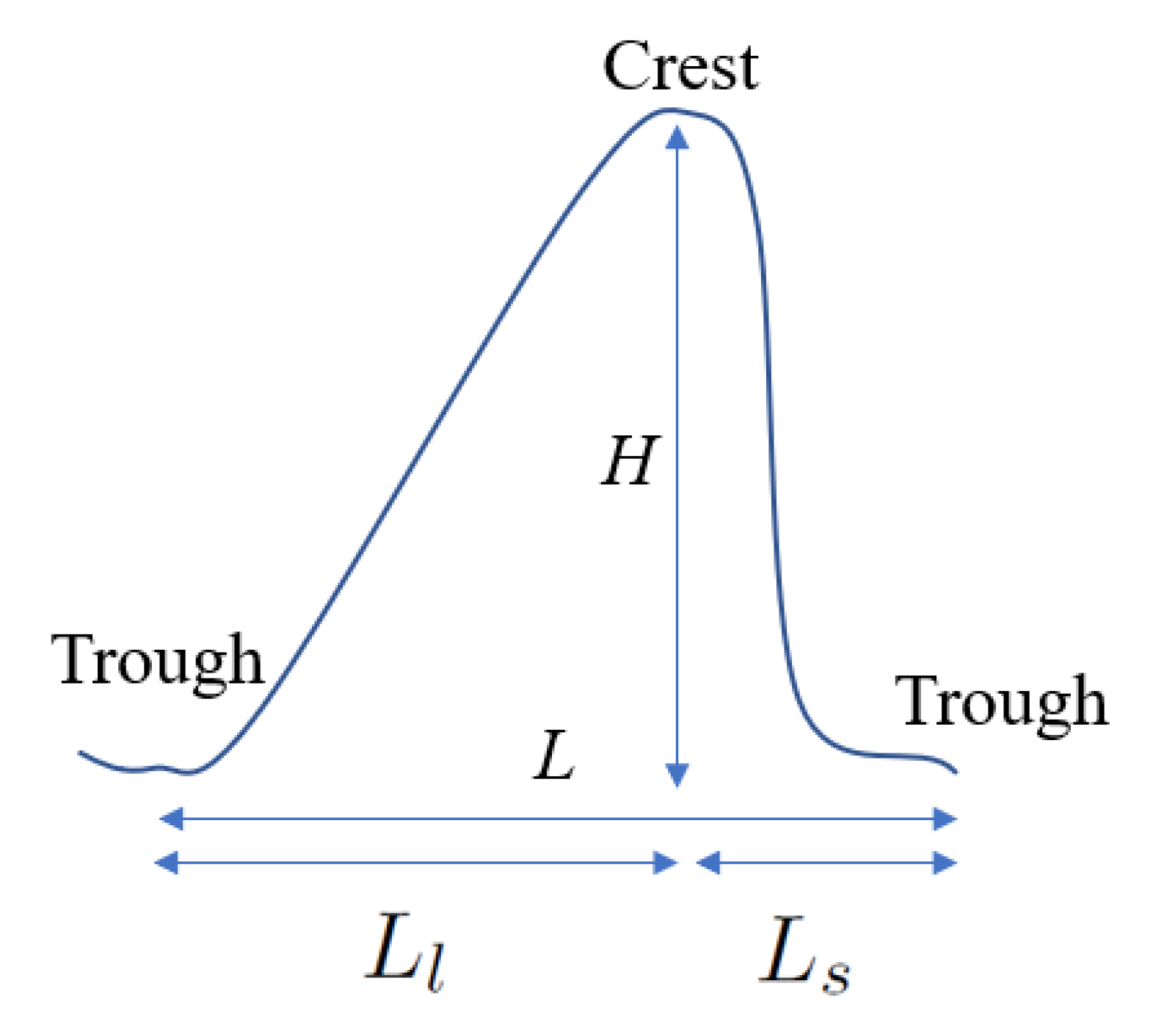
2.1.3. Sand Waves Area and Methods for Analysis

The multi-beam survey found large sand waves South of Clarke Island between South Head and Moriarty Point (Figure 4). These sand waves had their crest almost aligned perpendicular to the dominant tidal currents, with their key characteristics: wavelength, wave height and asymmetry (Figure 5) defined in

Table 2. Characteristics of the sand waves in Banks Strait south of Clarke Island.

Sand Waves	Wavelength (m)	Wave Height (m)	Asymmetry
SW1	902	13.4	−0.58
SW2	281	5.6	0.08
SW3	194	6.6	0.46
SW4	289	3.6	0.67

.

Crest and troughs were detected as local maxima and minima [7,57]. In this study, the wavelength was defined as the true length between two adjacent trough points, whereas wave height was defined as the difference between the crest level and the baseline of the two trough levels. (Equation (1)) and sand wave asymmetry were obtained with Equation (2) [58,59]:

$$H=z_{\mathrm{crest}}-\frac{z_s{L}_l+z_l{L}_s}{L}$$

(1)

$$A=\frac{L_l-L_s}{L}=\frac{\left|x_l-x_{\mathrm{crest}}\right|-\left|x_{\mathrm{crest}}-x_s\right|}{L}$$

(2)

with L as the wave length, $L_l$ the length of lee side and $L_s$ as the length of the stoss side (for symmetrical sand waves A = 0).

The height of the sand waves was between 10 and 36% of the water height, which is the range generally observed [60]. Three of the sand waves had heights larger than 5 m, corresponding to very large sand waves [61]. Most of the sand waves had asymmetry profiles with a steeper slope on the east side.

To further characterise the survey area, transects were undertaken in December 2018, using a sub-bottom (SB) profiling system. Georeferenced, sub-bottom data were acquired, using an acoustic profiling system (StrataBox 3510 HD, Syqwest Inc., Cranston, RI, USA) operating at 3.5 kHz. Transects were focused regions previously mapped for bathymetry and possible sandy sediment. Most of the sub-bottom data determined that the seafloor in the Banks Strait is largely homogenous rock or reef. However, the region to the South-East of the Clarke Island had a significant region of sand coverage on the seabed with the sand waves identified during the bathymetry survey. To compare the total load transport observed with the one from the numerical model, residual bed load sediment transport rates were calculated for the crest from the two data sets (multi-beam and sub bottom) over the 9 month period with the following:

$$q_{b_{obs}}=0.5H{V}_{mig}$$

(3)

where H is the height of sand waves and $V_{mig}$ is the migration speed [52].

Using the Soulsby-Van Rijn equations below for total load transport by waves plus current [52], the residual total load transport was estimated for the observations with the relation $A_{\mathrm{s}\mathrm{s}}/A_{\mathrm{s}\mathrm{b}}$ = 3.63, with $A_{\mathrm{s}\mathrm{b}}$ equal to $q_{b_{obs}}$ (Term $A_{\mathrm{s}\mathrm{s}}$ gave the suspended load transport). A factor of 2 was added in this relation, given that [52] indicated that bedform migration could underestimate the bedload transport by this factor. Then, this relation was reinjected into Equations (4) and (5) to obtain the total load rates:

$$q_{\mathrm{t}}=A_{\mathrm{s}}\overline{U}{\left[{\left({\overline{U}}^2+\frac{0.018}{C_{\mathrm{D}}}{U}_{\mathrm{rms}}^2\right)}^{1/2}-{\overline{U}}_{\mathrm{cr}}\right]}^{2.4}(1-1.6tan\beta )$$

(4)

with $\overline{U}$ equal to the depth-averaged current velocity, $U_{\mathrm{r}\mathrm{m}\mathrm{s}}$ the root-mean square wave orbital velocity, ${\overline{U}}_{\mathrm{c}\mathrm{r}}$ the threshold current velocity, $C_D$ the drag coefficient due to current alone and $\beta$ the slope of bed in streamwise direction.

where

$$A_{\mathrm{s}}=A_{\mathrm{sb}}+A_{\mathrm{ss}}$$

(5)

$$A_{\mathrm{sb}}=\frac{0.005h{\left(d_{50}/h\right)}^{1.2}}{{\left[(s-1)\mathrm{g}{d}_{50}\right]}^{1.2}}$$

(6)

$$A_{\mathrm{ss}}=\frac{0.012d_{50}{D}_{*}^{-0.6}}{{\left[(s-1)\mathrm{g}{d}_{50}\right]}^{1.2}}$$

(7)

$$D_{*}={\left[\frac{\mathrm{g}(s-1)}{{\nu }^2}\right]}^{1/3}{d}_{50}$$

(8)

$$C_{\mathrm{D}}={\left[\frac{0.40}{ln\left(h/z_0\right)-1}\right]}^2$$

(9)

where g is the acceleration due to gravity, h is the water depth, $\nu$ is the kinematic viscosity of water, s the relative density of sediment and $z_0$ the bed roughness length.

$${\overline{U}}_{\mathrm{cr}}=8.5{\left(d_{50}\right)}^{0.6}{log}_{10}\left(\frac{4h}{d_{90}}\right)\mathrm{for}0.5\le d_{50}\le 2\mathrm{mm}$$

(10)

$U_{\mathrm{r}\mathrm{m}\mathrm{s}}$ can be calculated from the parameters $H_{\mathrm{s}}$ (significant wave height), $T_{\mathrm{z}}$ (zero-crossing period of waves), and $T_{\mathrm{n}}$ (scaling period for waves) with the help of a curve derived from the JONSWAP spectrum [52].

$$T_{\mathrm{n}}=\left(h/{\mathrm{g}}^{1/2}\right)$$

(11)

$$T_{\mathrm{z}}=11{\left(\frac{H_{\mathrm{s}}}{\mathrm{g}}\right)}^{1/2}$$

(12)

The results are described in Section 3.1 and compared to the numerical results in Section 3.2.

2.2. Numerical Model

MIKE21 FM was used to model hydrodynamics and sediment transport in the area of the Banks Strait [44,62]. To model sediment transport, the module quasi three-dimensional “Sand Transport” (STPQ3D) was used, which determines the transport of non-cohesive particles (a common feature in high energy sites) based on both the hydrodynamic conditions (current and waves) and sediment properties [63]. The integrated momentum approach of [64] was used for the time evolution of the boundary layer, due to the combined wave-current motion. The mean bed shear stress was calculated from the turbulent boundary layer model and an additional constant velocity, found by iteration, was added to the wave orbital motion. Under the action of the wave and current, sediment transport rates were derived by linear interpolation of a sediment transport table using inputs from the hydrodynamic simulation. The bed load transport was calculated from the instantaneous Shields parameter using the Engelund and Fredsøe formula, with the suspended transport calculated as the product of the instantaneous flow velocities and sediment concentration [64,65]. When generating the sediment transport table, the model calculated bed and suspended load separately but saved only the total load to speed up the simulations; therefore, the description of sediment transport in this case was in equilibrium conditions. For the morphodynamic evolution of the bed, the Exner sediment continuity equation was solved at each timestep using the following:

$$-(1-n)\frac{\partial z}{\partial t}=\frac{\partial S_x}{\partial x}+\frac{\partial S_y}{\partial y}-\mathsf{\Delta }S$$

(13)

where n is the bed porosity, z is the bed level, t is the time, $S_x$ is the total load in the x direction, $S_y$ is the total load in the y direction and $\mathsf{\Delta }S$ is the sediment sink or source rate.

The numerical domain extended between 38${}^{\circ }$ S and 44${}^{\circ }$ S and 141${}^{\circ }$ E and 150${}^{\circ }$ E based on [47]. Near the model boundaries, mesh sizing of 3 km was used with resolution increasing at the approach of the Banks Strait with a sizing of 100 × 10 m for the area around the sand waves near Clarke Island. Sensitivity tests were performed for mesh size at the location of the sand waves, with a density of 10 m found to be the best compromise (time cost/accuracy) to represent the crests and troughs in the sand waves area as shown in Figure 6. The model data shoreline, bathymetry, wind data and open boundaries are detailed in

Table 3. Modelling parameters.

Vertical discretisation	2D
Shoreline	Geoscience Australia (GA)/Australian Hydrography Service(AHS) [67,68]
Bathymetry	GA/AHS/AUSTEn Project [45,67,68]
Tidal constituents	$S_1$, $K_1$, $O_1$, $P_1$,$Q_1$, $M_2$, $S_2$, $N_2$, $K_2$ and $M_4$ [69]
Wind/Sea level Pressure	ERA 5 [70]
Waves	Centre for Australian Weather and Climate Research (CAWCR) using Wawewatch III [66]
Validation	5 ADCP Measurements [47]

. Data sets from the Centre for Australian Weather and Climate Research (CAWCR) were used for the wave components with a spatial resolution of 4 km around Australian coastlines [66]. These data sets were used as a forcing in the sand transport module.

The models were run for the period of 16 March 2018 to 7 December 2018, with a one week spin up to match the data collected for sand waves migration (one survey in March 2018 with the multi-beam and one survey in the same area with transect conducted with the sub-bottom profiler in December 2018). A Barotropic model was used, given that the water column is well mixed and uniform in this energetic environment in the area [71]. For all simulations, the Manning value was set to 32 given the results of the sensitivity study of [47], representing a coarse sand habitat [52]. Sediment data were specified at a constant d50 of 0.8 mm (coarse sand) for the reference case. A sediment transport table was created based on the hydrodynamic characteristics of Banks Strait (

Table 4. Specifications of parameters for the sediment transport table.

Parameters	First Value	Value Max	No of Points
Current speed	0.1	4.1	20
Wave height	0.1	12.6	25
Wave period	1	29	14
Wave height/Water depth	0.05	20	20
Angle current/waves	0	360	12
Grain size	0.8	0.8	1
Sediment grading	1.1	1.1	1

) and served as a reference for the sensitivity tests. For the bed layer, an infinite supply of sediment was assumed as in [72].

Feedback between the evolving bed and the hydrodynamic model was included in the simulations to ensure dynamic interaction of the morphodynamic system. The bed evolution can be accelerated at each time step by means of a morphological speed up factor (SUF). A simulation of 1 month with a SUF of 10 represents 10 months. The reference scenario was compared to a simulation with a SUF of 20. Given that the difference was negligible (less than 0.01%) for the profile AA’ of the sand waves, this factor was applied to all sensitivity tests to optimize the computational time of 12 days to 20 h; all the tests are listed in

Table 5. List of sensitivity cases (SC).

	d50	Layer Thickness	Sorting	Manning	ST Formula	Waves Forcing	Tidal Current	Residual Current
Reference case	0.8	Infinite	1.1	32	cf. STQP3	Hs	Tides	Tidal
SC1	0.4
SC2	1.2
SC3	Varying
SC4		0 except sand waves area
SC5			1.3
SC6			1.62
SC7			2
SC8				28 in sand waves area
SC9				40 in sand waves area
SC10					Van Riijn Equilibrium	No
SC11					Van Riijn Non-Equilibrium	No
SC12					Engelund and Fredsøe Non-equilibrium	No
SC13							Tides × 2
SC14							Tides/2
SC15						Hs × 2
SC16						Hs/2
SC17								u + 0.005 m/s
SC18								u + 0.1 m/s

.

2.3. Hydrodynamic Model

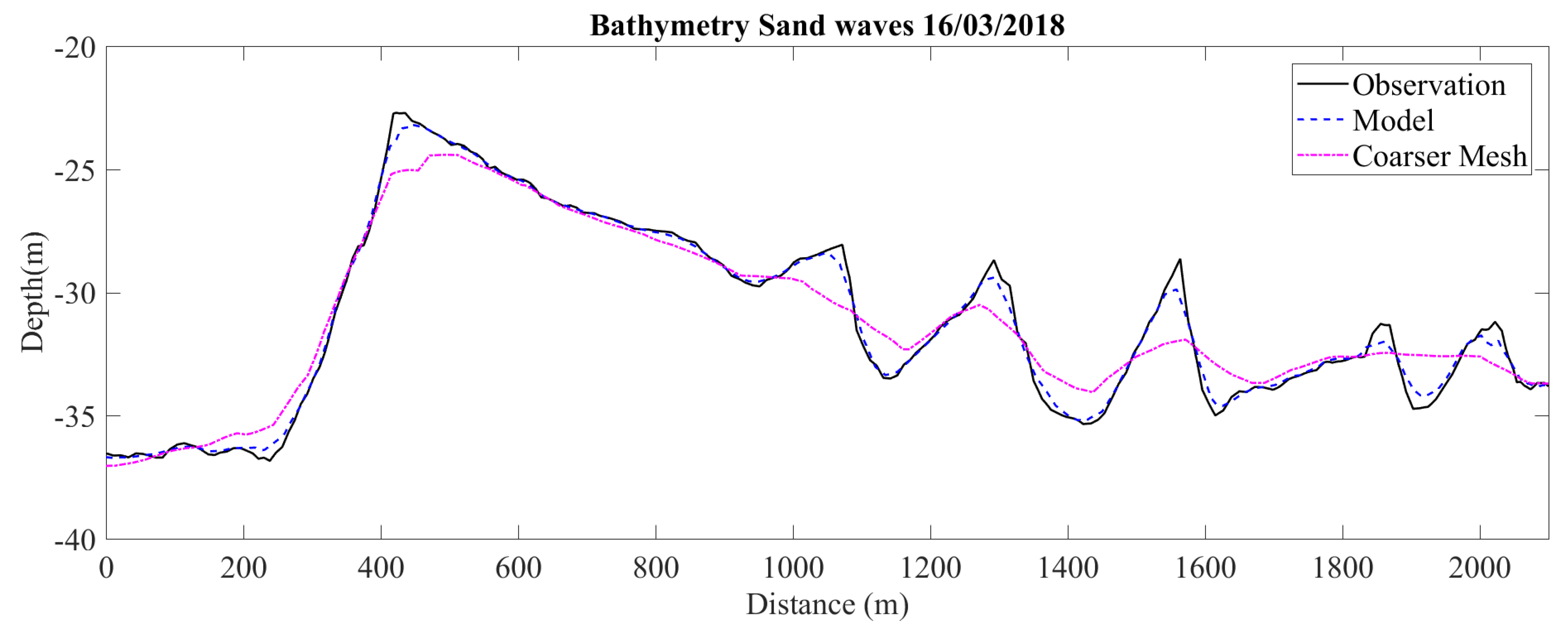
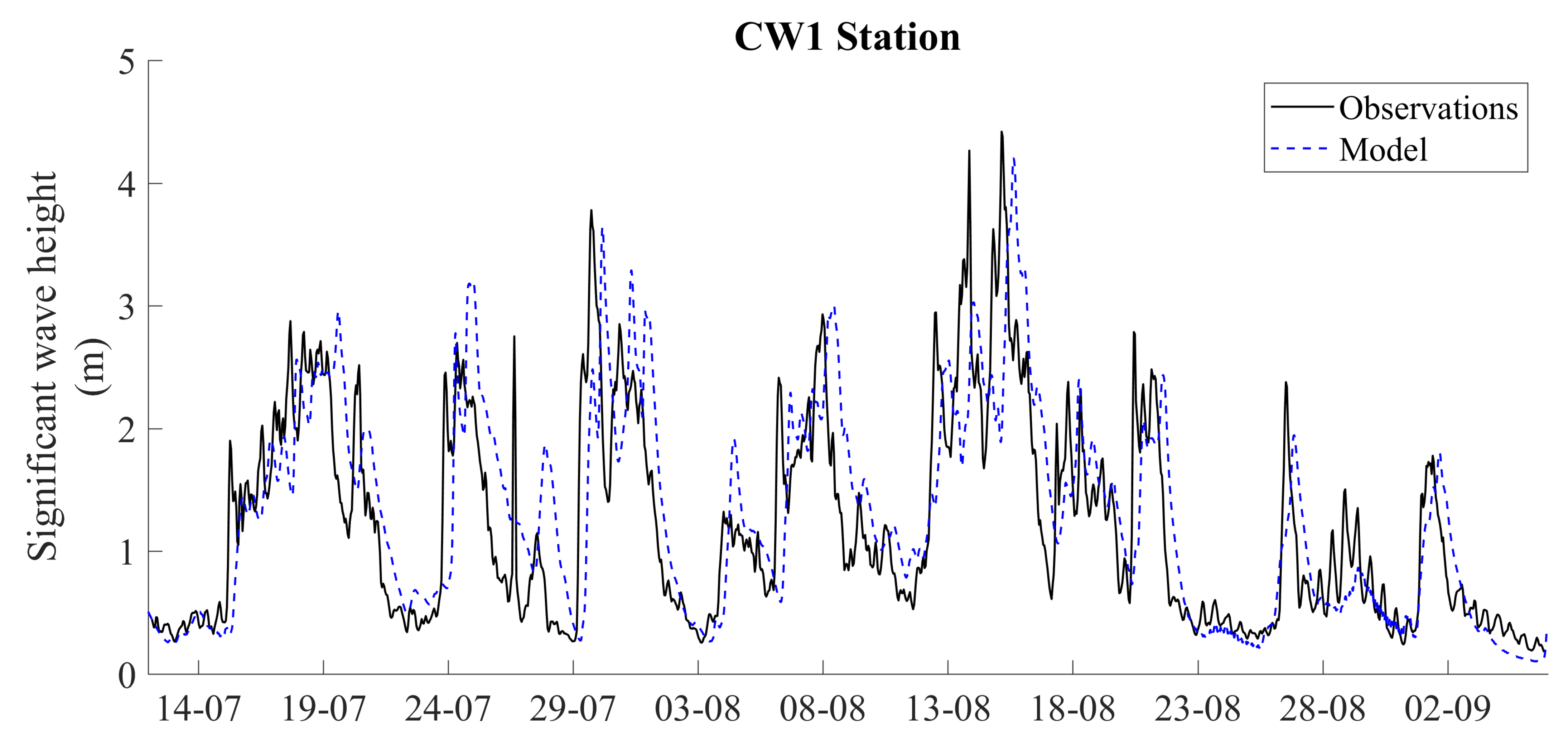
2.3.1. Validation of the Hydrodynamic Model

The model was calibrated and validated in a previous study with tidal forcing only [47] against five ADCP measurements, for 35 days and then for a whole year to assess the model for seasonal variations. Given the inclusion of waves in the model, as well as the slight alteration to the geographical extent and finer mesh in the key area, three statistics metrics (standard deviation, correlation coefficient and centered root mean square) were recalculated for depth-averaged velocities (DAV) to check the accuracy of the new domain (called R4 ND). Results showed good agreement with the field measurements and were slightly higher than the previously developed model (

Table 6. Comparison of statistics metrics (STD: m/s, R: unit-free, RMSE: m/s) for depth-averaged velocities between numerical models (R4: tidal current alone; R4 ND: waves + current) and field measurements for 35 days.

Stats	R4 [47] (Pure Current)	R4 ND (Waves + Current)
STD (0.403)	0.409	0.406
R	0.929	0.944
RMSE	0.153	0.135

and

Table 7. Comparison of Statistics metrics (STD: m/s, R: unit-free, RMSE: m/s) between numerical models and field measurements for autumn (22 March 2018 to 9 July 2018 for 3 ADCP) and winter (13 July 2018 to 6 September 2018 for 2 ADCP).

	Autumn			Winter
	STD (0.369)	R	RMSE	STD (0.279)	R	RMSE
R4 [47] Pure current)	0.384	0.922	0.149	0.302	0.861	0.155
R4 ND (Waves + Current)	0.38	0.943	0.127	0.299	0.908	0.126

).

A comparison between the model with waves forcing and the observations for the significant wave height (average height of the highest one-third of the waves) was performed, a slight time shift can be noticed, but overall the general pattern was reproduced. However, the model did not capture all the peaks which may lead to a difference in the sediment dynamic results (Figure 7).

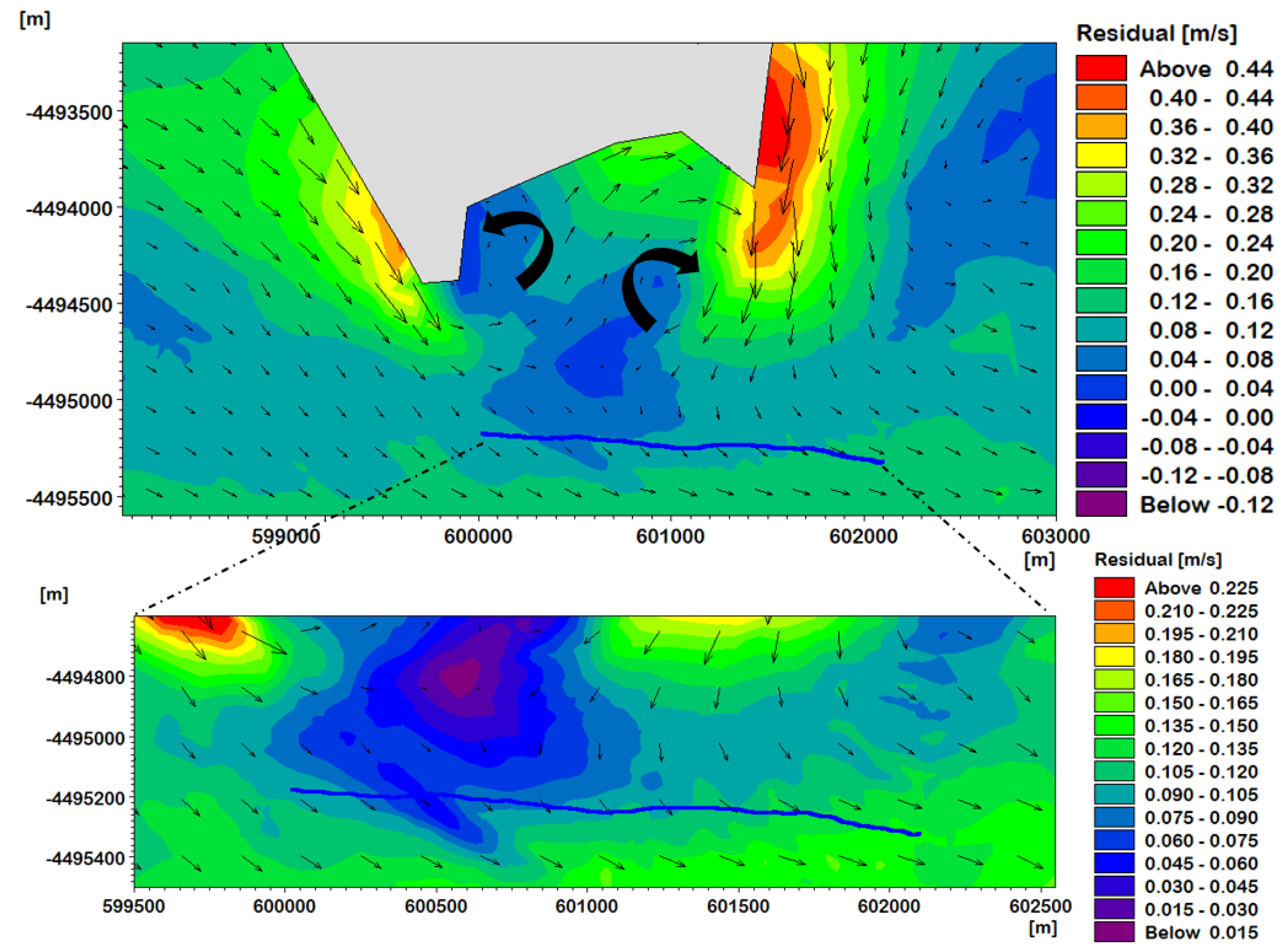
2.3.2. Estimation of the Residual current

The tidal residual current can be of significance for the movements of sediments and thus the migration of sand waves [73]. Residual currents were calculated from the ADCP data (

Table A4. Details of ADCP [47].

Name Station	Type of Instrument	Longitude	Latitude	Depth(m)	Date of Deployment	End of Data Collected
CW2	RDI Sentinel V50 500 kHz	148.10188	−40.5848	46.47	22/03/2018	11/07/2018
C1	RDI Workshorse 300 kHz	148.23882	−40.6727	57.94	17/03/2018	10/07/2018
CW3	Nortek AWAC 1 MHz	148.07778	−40.5454	34.95	22/03/2018	16/06/2018
CW4	Nortek AWAC 1 MHz	148.09241	−40.6664	30.67	15/03/2018	09/06/2018
CWTb1	Nortek Signature 500 kHz	148.22626	−40.6672	63.57	22/03/2018	09/07/2018
CW1	RDI Sentinel V50 500 Hz	148.05684	−40.5294	27.11	12/07/2018	06/09/2018
CW2 bis	RDI Sentinel V50 500 Hz	148.20132	−40.701	46.08	12/07/2018	22/09/2018
CW4bis	Nortek AWAC 1 MHz	148.34497	−40.7296	25.42	13/07/2018	08/09/2018
C1 bis	RDI Workshorse 300 kHz	148.12498	−40.6891	29.07	05/12/2018	15/02/2019

) and extracted from the simulations (

Table 8. Comparison of residual current between ADCP (location in Table A4) and numerical model.

			ADCP			Model
Period of Deployment		Stations	Residual (m/s)	Direction (Degree)	Cardinal Direction	Residual (m/s)	Direction (Degree)	Cardinal Direction
12 July 2018	6 September 2018	CW-1	0.063	246.6302	WSW	0.0626	265.8477	W
23 March 2018	9 July 2018	CW-2	0.085	119.2808	ESE	0.0564	143.5048	SE
23 March 2018	9 June 2018	CW-3	0.037	117.4155	ESE	0.0426	122.8949	ESE
23 March 2018	9 June 2018	CW-4	0.0534	257.946	WSW	0.0615	217.1545	SW
13 July 2018	8 September 2018	CW-4b *	0.0434	264.0938	W	0.0876	120.6333	ESE
23 March 2018	9 July 2018	CWTb-1	0.1453	130.2978	SE	0.101	142.7076	SE
23 March 2018	9 July 2018	C-1	0.118	132.6295	SE	0.1103	145.2016	SE
12 July 2018	18 September 2018	CW-2b	0.1082	156.8022	SSE	0.0657	155.9911	SSE

* outside of the channel.

). Results showed good correlation in the channel for the direction and the values were in the same range but weaker for most of the ADCP stations in the model. The observed residual currents account for the asymmetry of the tides as well as the residual large-scale circulation characterized by the sub-Antarctic surface water (SASW) or the East Australian Current (EAC) outside of the channel [74]. However, the simulations only accounted for tidal residual current, as no large-scale ocean circulation currents were applied at the boundaries. The analysis of residual current vectors from the simulation around the area of the sand waves indicated the presence of two eddies between Clarke Island and the sand waves (Figure 8). The residual direction was in the ebb direction towards the east, in the direction of the migration of the sand waves. The value of residual current in the area of the sand waves were slightly higher to those observed in the literature, such as in the North Sea, where Borsje [37] and Van Gerwen [38] used in their model a typical value of 0.05 m/s for residual current. According to [75], 10 percent of the observed residuals are in the range 0.15–0.25 m/s; the Banks Strait is, therefore, one of the few places with a high residual current.

3. Results

First the analysis of sand waves is presented. Secondly, the reference case scenario is analysed. Then, sensitivity studies are completed to investigate which parameters influence the most migration and are discussed.

3.1. Dynamics of the Sand Waves South of Clarke Island

The comparison between sand waves in March and December showed a distinct migration pattern of the sand waves towards the east, indicative of a dynamic sediment transport regime (Figure 9). To directly measure the long term migration rates and directions of sand waves would require several bathymetric surveys with multi-beam over a period of years which is not presently available. Caution, therefore, should be taken about the evolution of the sand waves here because for December, only one transect was available in the area. Migrations rates were quantified (

Table 9. Migration rates for sand waves.

Sand Waves	Migration Rate (Crest) for ∼9 Months (m)	Migration Rate (Trough) for ∼9 Months (m)
SW1	27.4	−25.4/99
SW2	135	87/99
SW3	21	7/87
SW4	−50	−7/−24

) using the equations described in Section 2.1.3. These results were comparable to other areas, such as tidal inlets. For example in the Marsdiep inlet (North sea) [76] found migrations rates up to 90 m/y and [20] an average of 32 m/y in the Gradyb inlet (Danish Wadden Sea). These rates were superior to rates in the coastal shelf: ref. [4] up to 8.8 m/y, ref. [6] up to 40 m/y, ref. [5] an average of 5.5 m/year and [7] up to 9 m/y. More recently, [15] found a migration of up to 70 m over a 50-day period in the Alderney South Banks, another promising tidal energy site.

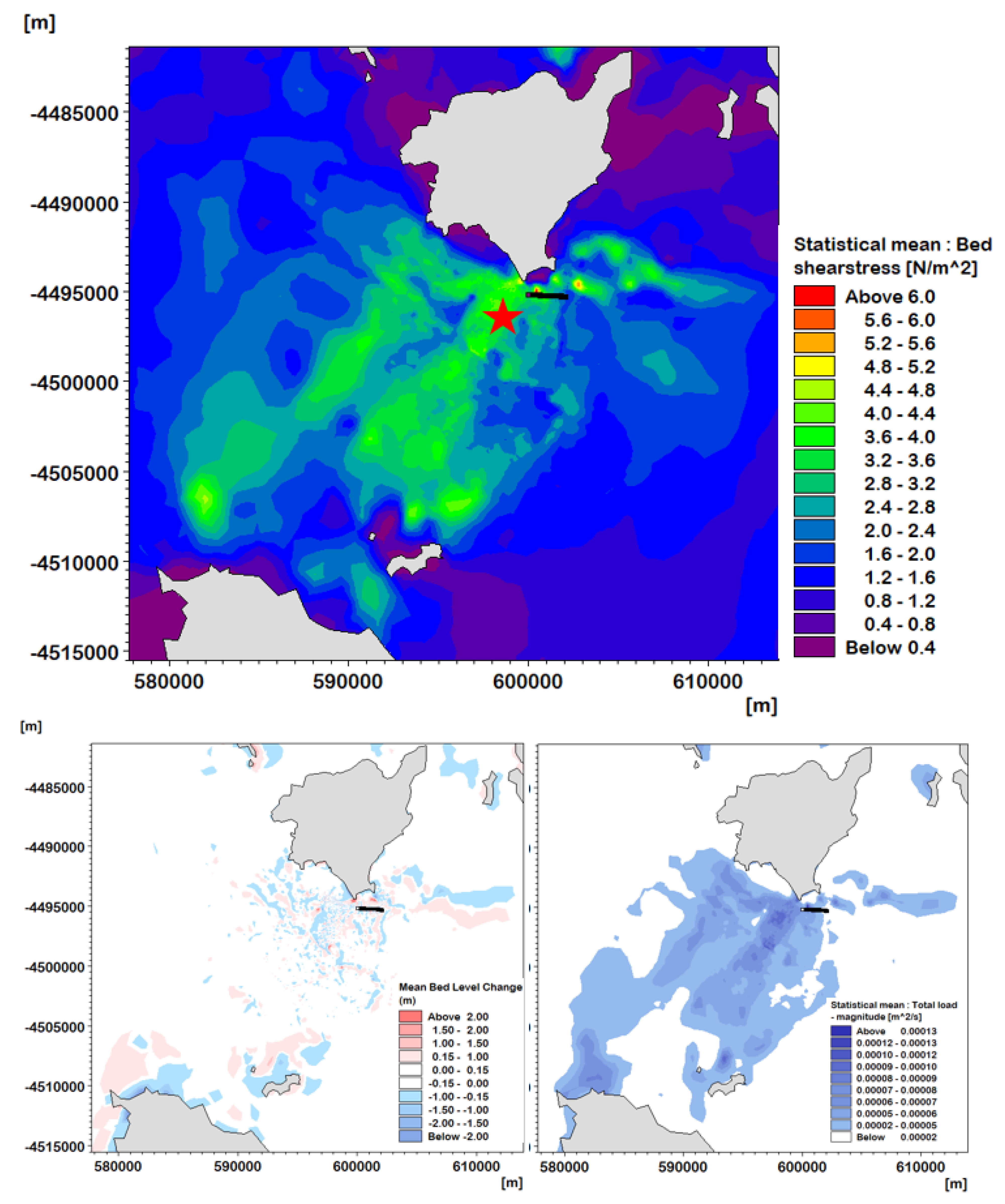
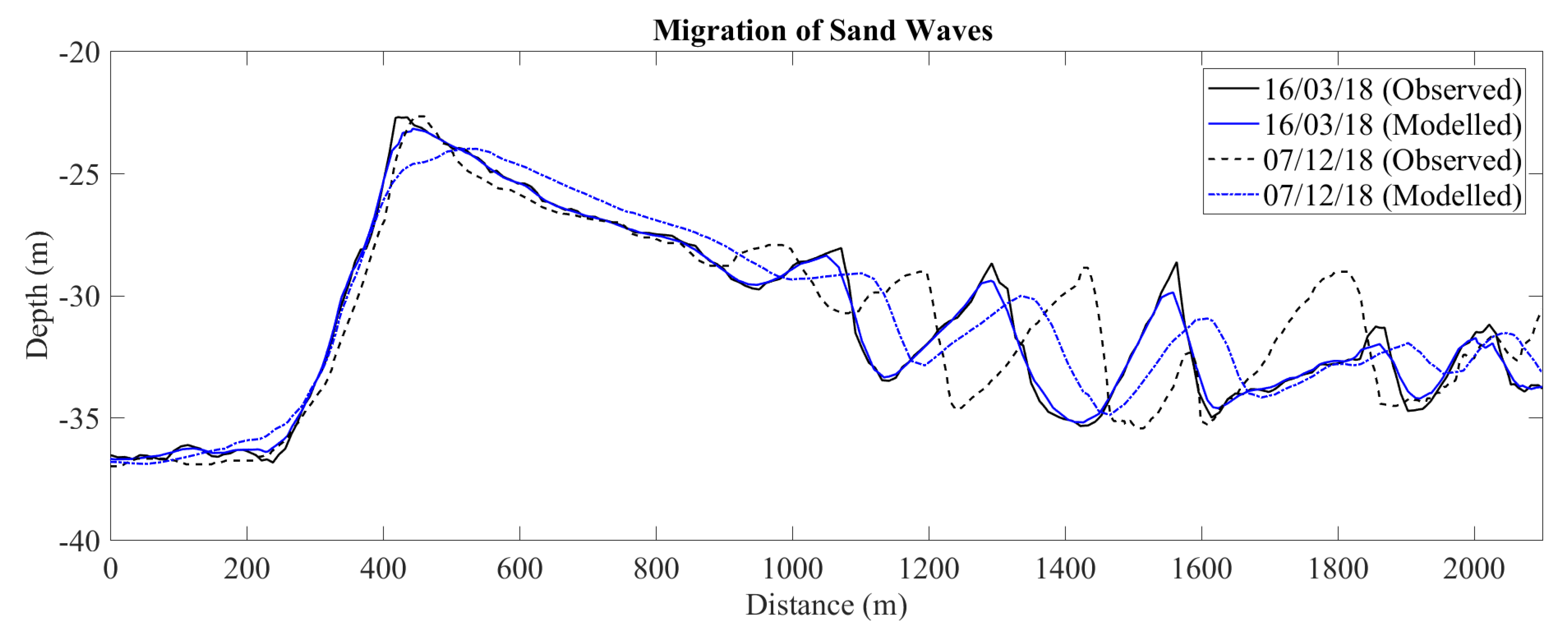
3.2. Reference Scenario

The model was developed to evaluate the sediment dynamics in the Banks Strait and the reference case revealed a high value of the mean bed shear stress, the principal parameter driving sediment transport (Figure 10). For coarse sand, the critical shear stress was in the range of 0.27–1.26 (N/m${}^2$) [77,78] and bed shear stress in Banks Strait exceeded this critical value. The bed level change map showed an erosion and accretion pattern in the sandy area south of Clarke Island and at the potential location of a tidal farm. The comparison of the two data sets of the AUSTEn project for the sand waves south of Clarke Island in 2018 (Figure 9) showed a migration towards the east, in accordance with the study of Slater [3] who showed that sediment transport rates in Banks Strait were in the east direction. For the reference scenario, migration in the eastward direction was also observed but with less migration than the observations (

Table 10. Characteristics of the sand waves modelled in the Banks Strait south of Clarke Island.

Sand Waves	Wavelength (m)	Wave Height (m)	Asymmetry	Migration Rate (Crest) for ∼9 Months (m)	Migration Rate (Trough) for ∼9 Months (m)
SW1	907	12.5	0.52	83.3	59.5/59
SW2	290	4.8	0.08	43	59/40
SW3	199	5.1	0.34	50	40/64
SW4	294	2.53	0.61	43	64/39

, Figure 11). Averaged values of bed shear stress in the range of 1.9 to 5.5 Pa were found along the profile AA’ with maximum values between 15 and 6 Pa, characterizing the high energetic site, which explained the high migration rates. This area was located near the eddies (Figure 8), at the corner of Clarke Island with residual flow from different direction and with more frictional interaction with the seabed.

A comparison between the total load transport rates estimated from observed crests migrations (total load rates from Equation (4)) and numerical model results were performed, with the results shown in

Table 11. Estimated total load magnitude for the crests of SW1 to SW4 (profile AA’).

${\mathit{Q}}_{\mathit{t}}$ (m${}^2$/d)	C1	C2	C3	C4
Model	9.08	3.71	2.92	2.02
OBS	1.03	0.63	0.03	−0.06
Equation (4)	11.4	2.5	1.46	0.67

. Sediment transport rates from the model did not match those estimated from the sand wave migration with a minimum of 80% of difference for C2 (crest of SW2) corresponding to 3.08 m${}^3$/day/m. Better agreement was observed by Blunden [15] in their studies of sand waves in the Alderney race, with a minimum difference of 4% (0.17 m${}^3$/day/m) and a maximum of 70% difference (2.27 m${}^3$/day/m), close to the minimum difference results here. Differences from 1.2 to 3 were found for the results between the model based on the equation of Engelund and Fredsøe and the Soulsby-Van Rijn equation (Equation (4)). The discrepancies between the rates calculated with Equation (4) and those estimated from the migrations of the sand waves were still very high with a minimum difference of 75% for C2. Using the migration of the sand waves to obtain the bed load rates was not conclusive in this case. The challenge for the observation in December was that only a sub-bottom transect was available not a full multi-beam survey, so an error margin (<15 m) could exist for the exact position of the sand waves.

The only direction pattern not reproduced in the propagation of sand waves in the model was the migration of SW4. Observations showed an increase of the sand waves, which was not captured by the model. This could be explained by the change of directions observed in the residual current, residual sediment transport and in the orientation of the sand waves at this particular location (Figure 8 and Figure 12). This increase in the sand wave height could also be related to a dominant bed load transport in this area. Moreover, the model did not reproduce well the peaks of large waves during storm events, which may also explain the discrepancies for the sediment transport rates. Large waves or swell resulting from storms may affect the magnitude and direction of sediment transport for a short period [73]. The region further north of the sand waves was not surveyed and unknown topographic features may also influence the magnitude of the current. Moreover, the model was not forced with large-scale ocean circulation at the boundaries, which might influence the results. The observed migrations highlighted how the large-scale circulation combined with asymmetry of the tides and waves interaction was important in this area, which may not be the case for other areas such as the Alderney race in the English Channel. Nevertheless, the model showed a migration in the correct direction for the sand waves. Sensitivity experiments were performed to further analyse the major driver of sand wave migration and to determine whether the model results could be improved.

3.3. Sensitivity Tests: Morphology

The reference scenario was compared to sensitivity tests with varying grain size, distribution (constant or varying), sorting of sediment and differencing bed frictions.

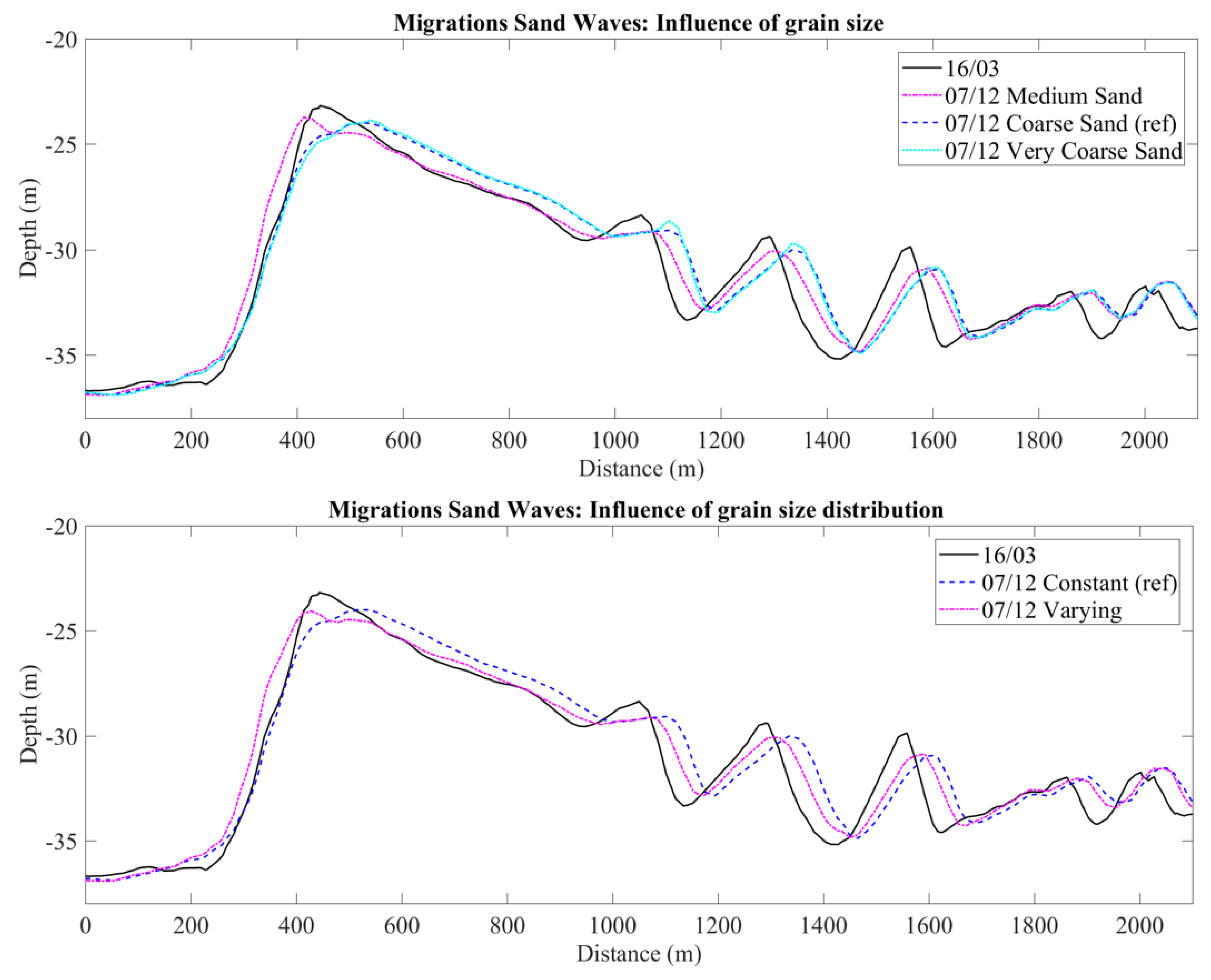
3.3.1. Influence of the Median Grain Size (d50)

The migration of sand waves using a d50 of 0.4 mm (medium sand), 0.8 mm (coarse sand, reference scenario) and 1.2 mm (very coarse sand) with a sorting of 1.1 are shown on Figure 13. This range of values was found during the AUSTEn surveys in the Banks Strait. The sediment grain size altered the evolution of the sand waves, with differences noticed between the different classifications. Coarse and very coarse sand showed the same pattern for the evolution of the sand waves with a smaller increase in the crests for coarser sand. For finer sand, the sand wave heights were flattened, certainly due to an increase of erosion of crests and deposition away from the sand waves, resulting from the high velocity fine particles, which are easily lifted up and can be transported further. This was in accordance with the findings of [5]. For coarse and very coarse sand, the difference was negligible; the migration for medium sand was 55% slower than the coarse sand case.

3.3.2. Grain Size Distribution

An interpolation of sediment samples was performed to test whether more detailed information on sediment distribution and grain sizes in the area was necessary. For this distribution map of sediment, 1085 samples of seabed sediment (AUSTEn project and Marine Sediments Database [45,54]) were used to interpolate median grain size with the Inverse Distance Weighting method (Figure A1 in Appendix A). The varying grain size model resulted in less migration towards the east than the reference scenario, with 76% less migration for the sand wave SW2 than the reference case (Figure 13).

3.3.3. Layer of Thickness

The SB data showed that the seafloor in Banks Strait is largely homogeneous rock or reef, except in the area of sand waves. However, the layer thickness of sediments above bedrock in the Banks Strait could not be determined precisely and seemed to vary according to the SB survey. As a result, an infinite supply of sediment was chosen for the reference scenario (also the default case in MIKE21). To try to reproduce a scenario with bedrock and the sandy area, the simulation SC4 was set with a non-erodible layer, except at the location of the sand waves where 5 m was chosen for the area of SW2–SW4 and 12 m for SW1 (value estimated from the SB survey). The migration of the sand waves was slower with a non-erodible layer around the sand waves (Figure 14). Berthot [79] tested 2 m and 4 m of availability of sand in his model for the evolution of sandbank and showed that when the layer thickness was smaller, the evolution was slower.

3.3.4. Sorting

Sorting values of 2 to 1.1 (reference case) were varied to determine their influence on the migration of sand waves. The value of 2 corresponded with poorly sorted, 1.62 for the limit between poorly and moderately sorted [52], 1.3 was chosen to see the sensitivity in the range of well sorted sediment, and 1.1 was the default case in MIKE21. All the values tested gave higher migration rates for SW2 crest, compared to the reference case. When the sediments were more mixed, the evolution was faster, with the migration rates being very sensitive to this sorting parameter (Figure 14).

3.3.5. Bed Friction

The bed friction represented in the model by the Manning number (M) was modelled with a constant value of 32 (from the calibration of [47]) for the whole domain for all of the runs, except for two simulations where the Manning number was modified just at the location of the sand waves with the value of 28 for SC8 and 40 for SC9. With a smoother bed (M = 40) at the location of the sand waves, the migration rates for SW2 were two times higher compared to the reference case approaching the observed rates and shape (asymmetrical) (Figure 14). With a smaller Manning number (M = 28), the evolution of sand waves for SW2 was almost twice as small compared to the reference case and slightly more symmetrical. A smaller Manning number induced an increased bed shear stress, leading to more turbulence and possibly more suspended load transport which could explain the slower evolution.

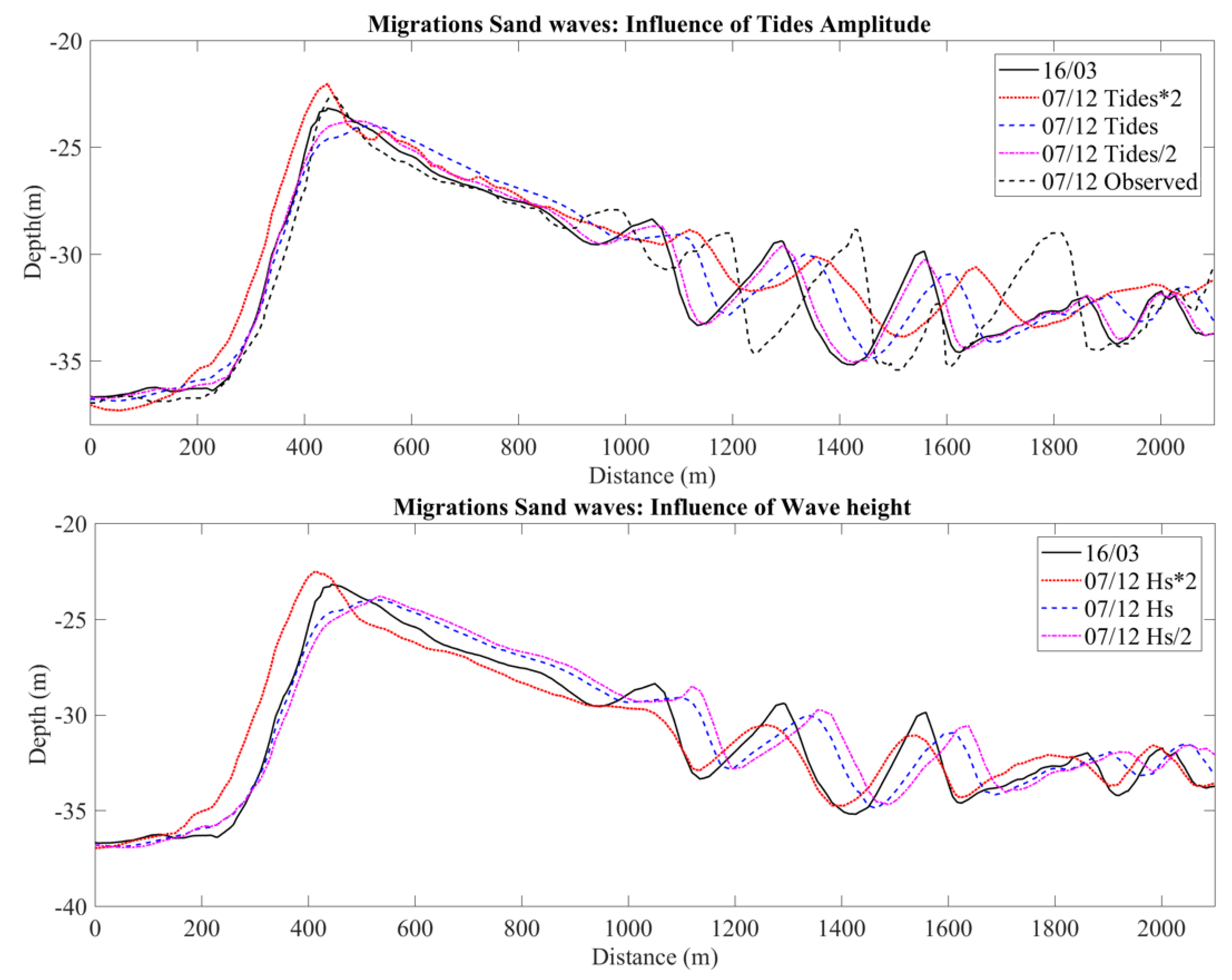
3.4. Sensitivity Tests: Tides & Waves, Pure Current

The reference scenario (wave and current) was compared to simulations without wave forcing (SC10/11/12) for the period of 9 months. For the pure current cases, three different sediment transport formulae were tested: Van Rijn (VR) equations [60,80] in equilibrium and non-equilibrium mode and Engelund and Fredsøe (EF) [65] in non-equilibrium mode. The EF formula in equilibrium mode was not tested, given the instability [81] found in their sensitivity tests for energetic sites. For the three cases with current forcing only, the migration of crests and troughs was not well represented as shown in Figure 13. The sand waves were totally flattened, and the bottom of the seabed was lower with the EF formula. Auguste [81] found that the EF formula was more sensitive to basic physical properties, such as strong currents, than the VR formula and may not be suitable in a highly energetic site. For the reference scenario (wave + current) the depth-averaged current was reduced up to 0.1 m/s with an average reduction of 0.02 m/s for the profile AA’. The wave–current interaction is important in the Banks Strait [82] and thus simulations with just tidal current alone are not relevant here for investigating the evolution of the sand waves as shown in Figure 15 with the flat lines for pure current.

Another sensitivity test was carried out to investigate the influence of tidal amplitude on the migration of sand waves. The amplitude for this test case was modified by a factor of two when compared to the reference scenario (Figure 16). Higher amplitude showed larger migration of the sand waves towards with east (+68% for SW2) with more deposition in the troughs, inducing a reduction in the sand wave height. The smaller amplitude resulted in almost no migration of the sand waves, with a slight reduction in the sand wave height compared to the initial state (16/03); the results were comparable to the study of [38] for a reduction of the amplitude of symmetrical tide.

For the significant wave height (Hs), the same sensitivity tests were performed with a factor of 2 (Figure 16). No migration was observed for the sand waves with higher waves; the crests were flattened, except for SW1. Increasing waves height involved more turbulence and increased the bed shear stress compared to the reference case +17% along the profile AA’. In this shallow area, the amount of sediment lifted into suspension was greater with the higher wave height, which may have led to greater suspended load transport and deposition in other locations. This was in accordance with the findings of Tonnon [5] who showed no migration for the artificial sand waves, due to the increasing stirring effect with increasing waves. The reversal of SW1 can be explained by the dominance of the waves on the tides in case of higher waves as King [40] suggested in his study. Smaller waves led to higher crests and more migration towards the east. Smaller waves enhanced sand transport in the residual direction, and there was an increase in the total load transport of +87% along the profile AA’, compared to the reference case.

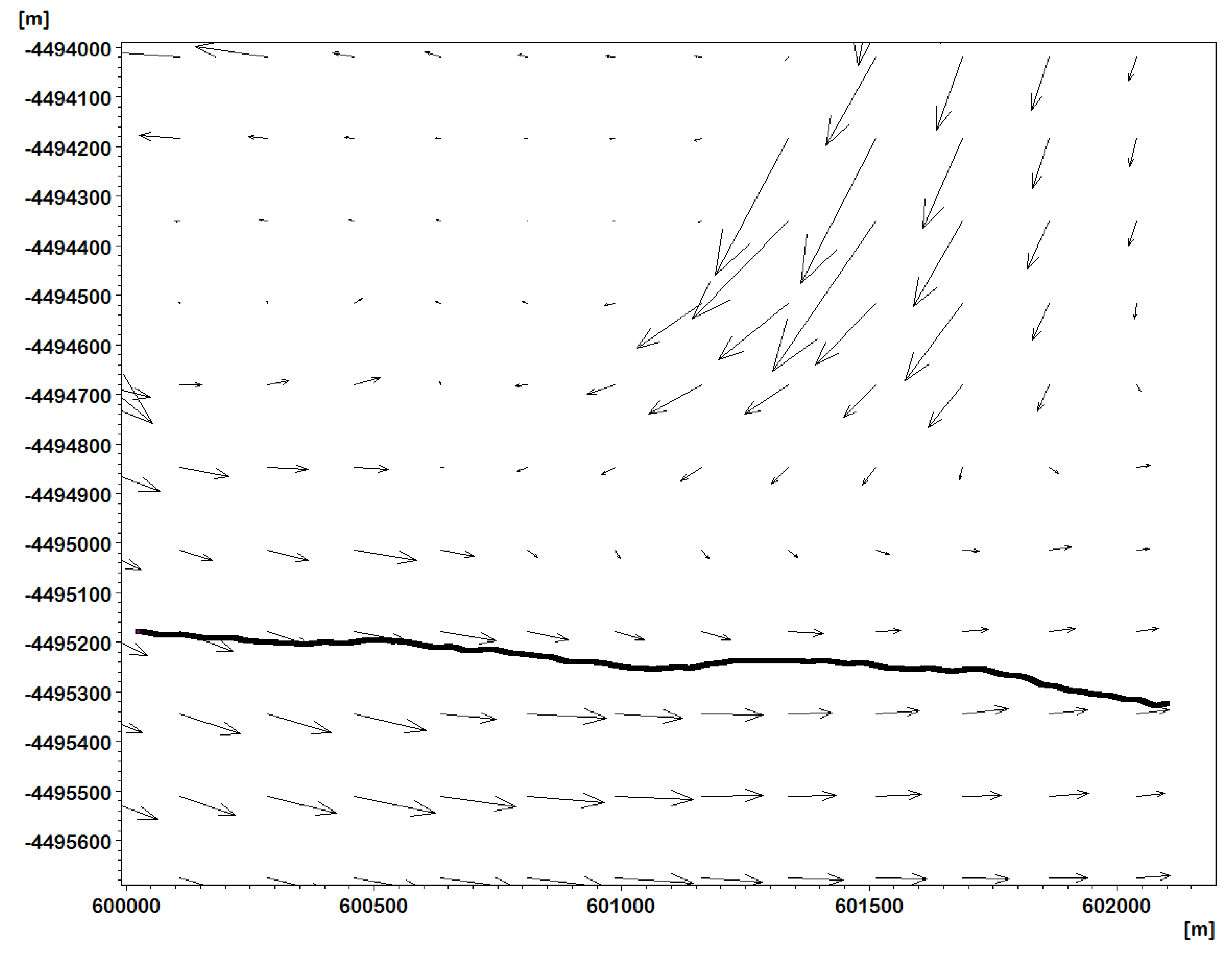
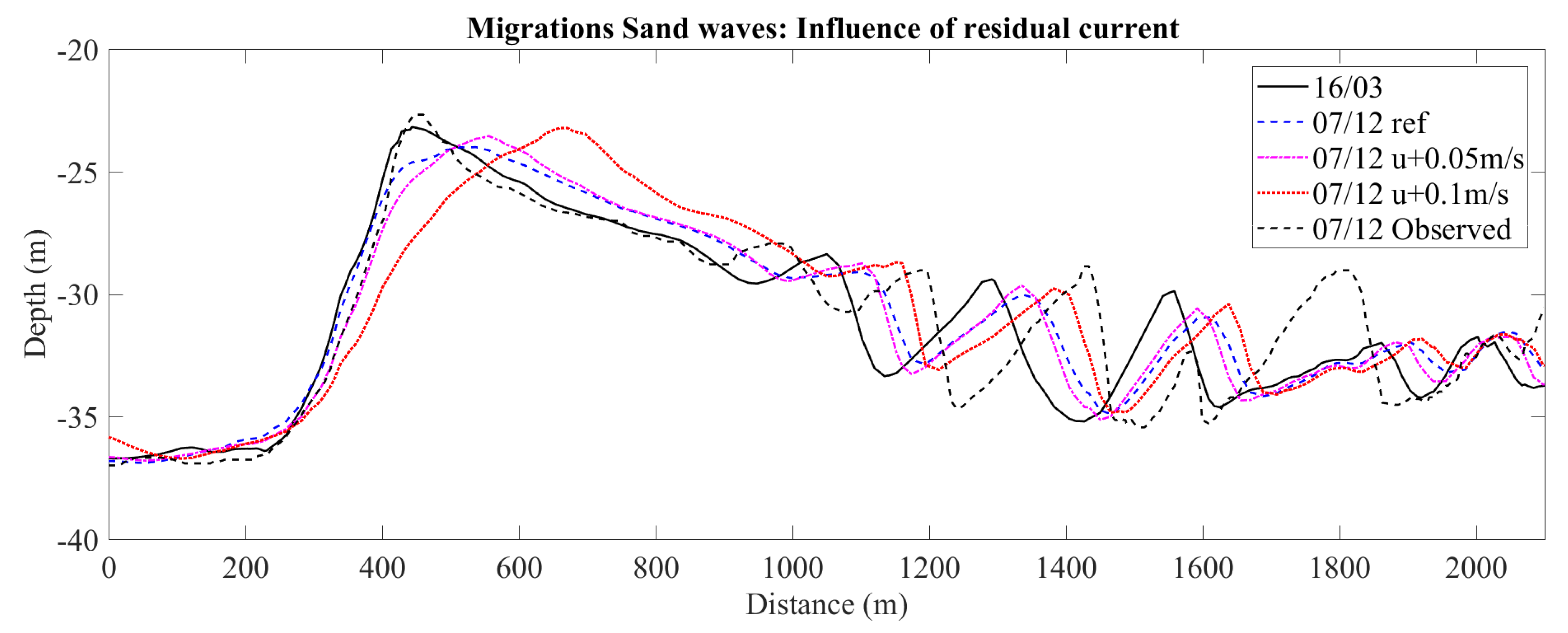
3.5. Sensitivity Tests: Residual Current

The residual current is one of the dominant factors for the migration of the sand waves. In order to determine the influence of the magnitude of residual current on the evolution of sand waves, a residual current was added to the tidal residual. In Section 2.3.2, the difference between ADCP residual and tidal residual from the model were measured with a maximum of 0.05 m/s. Thus, the value of 0.05 m/s was added in the forcing for the u component, and the double of this value was also tested. The sand waves migrated more towards the east approaching the observed rates for the high (+0.1 m/s) residual model (SC18), with an increase to the east of 47 m compared to the reference scenario for the crest of SW2. For the value of 0.05 m/s, the evolution was quite similar to the reference scenario with an increase of 0.6 m for the height of SW2 crest (Figure 17). A constant value for the residual current was added in this study, but residual currents vary seasonally, and the direction of the added component may also be important for the evolution of the sand waves [73].

3.6. Summary and Recommendations

3.6.1. Summary of Sensitivity Experiments

In the Banks Strait, the migration of sand waves was studied, and special attention was given to the influence of several parameters on the migration: properties of sediment (grain size, spatial distribution of sediment, layer thickness for the seabed, sorting of sediment and bed friction) and hydrodynamics (pure current, amplitudes of tides, height of significant wave and value of residual current) (Table 5). Various model parameters were found to affect the migration of sand waves.

The cases of pure current (SC10/11/12) showed flat lines for the migration of sand waves, highlighting the importance of the wave–current interaction for sediment dynamics in the Banks Strait. Compared to tidal forcing alone, the combined wave–current model generates more turbulence from the wave boundary layer and from energy dissipation, due to wave breaking. More sediment is available to influence the sand wave migration. Spatial distribution of the grain size (SC3) and the non-erodible layer case (SC4) revealed less migration compared to the reference case. Variations of grain size (SC1/2) displayed similar results for coarse and very coarse sand but were two times slower for medium sand. Identification of the classification (Wentworth scale [51]) of sediment is an important element especially if finer sand is the dominant component. Amplitude of tides (SC13/14) and waves (SC15/16) modify the propagation of the sand waves and the dynamic of sediment with more migration than the reference case for higher values.

Of all the sensitivity tests cases, only three showed migration rates approaching the observed rates especially for SW2: poorly sorted sediment (SC7), mixed bed friction with a constant value in the domain and a higher value in the sand waves area (SC9) and an added value of 0.1 m/s for the residual current (SC18).

For the case of SC7 (poorly sorted sediments), the sediments were more mixed and thus reacted differently to critical bed shear stress. With an increase in the grading coefficient, finer fractions were suspended and coarser fractions moved, as the bedload had a greater tendency to settle. More migration was observed compared to the reference case, certainly due to an increase in the deposition rates. Values between 2 and 1.62 may correspond to the sorting representation for the 12 AUSTEn samples, but more detailed in situ data are needed to optimize the value of this coefficient and were not available. Further processes that could be investigated is the separation of the sand waves in different size fractions; observations have mostly found coarser sediment on the crests and finer in the troughs as discussed by Roos [8] and Van Oyen [34]. For this analysis, more sediment samples are needed at the location of the sand waves.

Simulation using a higher Manning coefficient value in the sand waves area (SC9) led to migration rates twice as great as those of the reference scenario. Using less friction in the model domain and thus less turbulence in this area could have implied more deposition. The hydrodynamic model was validated with a constant value of M = 32 [47]. However, a variable bed roughness should be tested in future work to see the influence of the distribution on the validation, ideally by using more in situ sediment and current data in proximity to the area to refine the validation process. For current data, this is a challenging task, given that two ADCP frames were buried and could not be retrieved at the location of the sand waves. Boat mounted ADCP can be used in future surveys to overcome this difficulty.

Increased residual current (SC18) resulted in an increase in the migration of the sand waves towards the east, with model results close to the measured migration rates of SW2. The tidal asymmetry is not the only driver of the sand wave migration. It is a combined effect of tidal asymmetry and large-scale ocean circulation. Further investigations about the variations of the residual current in this area or inclusion of large-scale ocean circulation at the boundaries could potentially lead to better agreement with observations but are outside the scope of this study.

3.6.2. Recommendations for Future Field Work

Based on these results, future field work should aim at deploying the instruments listed in

Table 12. Recommendations for “Ideal” field surveys for tidal energy.

	High Energetic Site		High Energetic Site with Known Bedforms
	Limited Budget	Desired	Limited Budget	Desired
Multi-beam survey	x		x
Several multi-beam surveys (3 years)				x
Grab sampler/Sediment trap	x		x	x 1
Penetrometer		x		x
Sub-bottom profiler			x
ADCP (90 days of data)	x		x
ADCP (1 year of data)		x		x

¹ in the crests, troughs, and along the slopes of the bedforms.

to collect data for preliminary environmental impact assessment for tidal energy sites, in complement to the EMEC/IEC-TS guidelines [83,84]. This will help tidal project developers and researchers to prepare while reducing cost for future campaigns for potential tidal sites.

3.6.3. Recommendations for Numerical Modelling

For numerical modelling, the authors recommend the following parameters for preliminary morphological assessment:

• Constant grain size identified as the most typical for the area considered based on the Wentworth scale/ISO 14688 [85].
• Optimized value of sediment sorting of sediment (if a large set of sediment samples is available).
• Infinite supply for the layer of thickness for a first approximation.
• Spatial distribution of bed friction coefficient (if a large set of in situ data is available).
• The site’s exposure to waves should be assessed when analysing sediment transport, especially in the presence of bedforms, such as sand waves. If the wave–current interaction is important, wave forcing or a coupled wave/current model should be considered.
• Ocean circulation forcing at the boundaries, if a larger model is available.

4. Conclusions

A high resolution 2D hydrodynamic–morphodynamic model with wave forcing was used to explore the dynamics of sediment transport and of sand waves located in the Banks Strait, a promising site for tidal arrays deployment in Australia. The hydrodynamic model was validated against a large data set of ADCP data with good agreement for the depth average velocities and elevations. Averaged bed shear stresses for the whole period showed high rates largely higher to the critical value for coarse sand, highlighting the turbulent environment in this area. The area of South Clarke Island is very energetic, as evidenced by the silting of two ADCP frames up to 1 m within 5 months. Migration rates in excess of one hundred meters for the period of deployment (9 months) were found in the Banks Strait and were superior to the values usually found in the literature (several meters by year) for other sites. The developed model was able to reproduce migration patterns towards the east; however, the model produced smaller sand wave evolution rates compared to the observation. Long-term surveys on the scale of years/decades would indicate the validity of these shorter-term observations.

For preliminary environmental assessment in tidal energy sites, in situ data sets are necessary to validate the hydrodynamics and have insight about the sediment properties. The study investigated the parameters that mostly drive sediment transport under the action of waves and current and uses sand waves migrations south of Clarke Island to perform sensitivity testing. The sensitivity tests showed that sorting, bed roughness and residual current were key factors to the migration of the sand waves, whilst grain size, amplitude of tides and waves revealed weaker impact on sand wave migration. The migration of the sand waves in Banks Strait is strongly linked to the hydrodynamics, therefore any changes to the hydrodynamic conditions, such as tidal energy extraction may alter the sediment dynamics. The numerical model was run with wave forcing. Further work should investigate the difference between this approach and a fully coupled spectral wave/hydrodynamic/sand transport model. The full coupled model may give better agreement since it may better capture higher peaks in waves heights during extreme events, which are significant for sediment dynamics.

This paper gives new insights into the seafloor characteristics in this area and provides crucial information for tidal projects developers: an increased knowledge of the substrate type for turbines foundations and an assessment of natural sediment activity for future turbines deployments. Further studies using this model are in progress to investigate the influence of tidal stream energy extraction on the morphology of the Banks Strait and especially the migration of sand waves.

References

1. Nash, S.; Phoenix, A. A review of the current understanding of the hydro-environmental impacts of energy removal by tidal turbines. Renew. Sustain. Energy Rev. 2017, 80, 648–662. [Google Scholar] [CrossRef]
2. Copping, A.; Hemery, L. OES-Environmental 2020 State of the Science Report: Environmental Effects of Marine Renewable Energy Development Around the World; Report for Ocean Energy Systems (OES); Technical Report; U.S. Department of Energy: Washington, DC, USA, 2020.
3. Slater, R. Marine Geology of Banks Strait-Furneaux Islands Area, Tasmania. Ph.D. Thesis, University of Sydney, Sydney, Australia, 1969. [Google Scholar]
4. Besio, G.; Blondeaux, P.; Brocchini, M.; Vittori, G. On the modeling of sand wave migration. J. Geophys. Res. C Ocean. 2004, 109, 1–13. [Google Scholar] [CrossRef] [Green Version]
5. Tonnon, P.; van Rijn, L.; Walstra, D. The morphodynamic modelling of tidal sand waves on the shoreface. Coast. Eng. 2007, 54, 279–296. [Google Scholar] [CrossRef]
6. van Dijk, T.; van der Tak, C.; de Boer, W.; Kleuskens, M.; Doornenbal, P.J.; Noorlandt, R.; Marges, V. The Scientific Validation of the Hydrographic Survey Policy of the Netherlands Hydrographic Office, Royal Netherlands Navy. Technical Report. 2011. [Google Scholar]
7. Knaapen, M. Measuring sand wave migration in the field. Comparison of different data sources and an error analysis. In Proceedings of the Marine Sandwave and River Dune Dynamics II, Enschede, The Netherlands, 1–2 April 2004; pp. 152–159. [Google Scholar]
8. Roos, P.; Hulscher, S.; Meer, F.; Wientjes, I. Grain size sorting over offshore sandwaves: Observations and modelling. In Proceedings of the 5th IAHR Symposium on River, Coastal and Estuarine Morphodynamics, Enschede, NL, USA, 17–21 September 2007. [Google Scholar] [CrossRef]
9. Bellec, V.K.; Bøe, R.; Bjarnadóttir, L.R.; Albretsen, J.; Dolan, M.; Chand, S.; Thorsnes, T.; Jakobsen, F.W.; Nixon, C.; Plassen, L.; et al. Sandbanks, sandwaves and megaripples on Spitsbergenbanken, Barents Sea. Mar. Geol. 2019, 416, 105998. [Google Scholar] [CrossRef]
10. Hoozemans, F.M.J. Horizontale ZandgolvenL Literatuurstudie; Technical Report; Deltares, Hydraulic Engineering Reports: Delft, The Netherlands, 1991. [Google Scholar]
11. Daniell, J.J.; Harris, P.T.; Hughes, M.G.; Hemer, M.; Heap, A. The potential impact of bedform migration on seagrass communities in Torres Strait, northern Australia. Cont. Shelf Res. 2008, 28, 2188–2202. [Google Scholar] [CrossRef]
12. Katoh, K.; Kume, H.; Kuroki, K.; Hasegawa, J. The development of sand waves and the maintenance of navigation channels in the bisanseto sea. Coast. Eng. 1998, 1, 3490–3502. [Google Scholar] [CrossRef]
13. Malikides, M.; Harris, P.T.; Jenkins, C.J.; Keene, J.B. Carbonate sandwaves in Bass Strait. Aust. J. Earth Sci. 1988, 35, 303–311. [Google Scholar] [CrossRef]
14. Zhou, J.; Wu, Z.; Jin, X.; Zhao, D.; Cao, Z.; Guan, W. Observations and analysis of giant sand wave fields on the Taiwan Banks, northern South China Sea. Mar. Geol. 2018, 406, 132–141. [Google Scholar] [CrossRef]
15. Blunden, L.S.; Haynes, S.G.; Bahaj, A.S. Tidal current power effects on nearby sandbanks: A case study in the Race of Alderney. Philos. Trans. R. Soc. A Math. Phys. Eng. Sci. 2020, 378, 20190503. [Google Scholar] [CrossRef]
16. Santoro, P.; Fossati, M.; Tassi, P.; Huybrechts, N.; Van Bang, D.P.; Piedra Cueva, I. A coupled wave-current-sediment transport model for an estuarine system: Application to the Río de la Plata and Montevideo Bay. Appl. Math. Model. 2017, 52, 107–130. [Google Scholar] [CrossRef]
17. Barnard, P.L.; Hanes, D.M.; Rubin, D.M.; Kvitek, R.G. Giant sand waves at the mouth of San Francisco Bay. Eos Trans. Am. Geophys. Union 2006, 87, 285–289. [Google Scholar] [CrossRef]
18. Dalrymple, R.W.; Knight, R.J.; Lambiase, J.J. Bedforms and their hydraulic stability relationships in a tidal environment, Bay of Fundy, Canada. Nature 1978, 275, 100–104. [Google Scholar] [CrossRef]
19. Buijsman, M.C.; Ridderinkhof, H. Long-term ferry-ADCP observations of tidal currents in the Marsdiep inlet. J. Sea Res. 2007, 57, 237–256. [Google Scholar] [CrossRef]
20. Bartholdy, J.; Bartholomae, A.; Flemming, B. Grain-size control of large compound flow-transverse bedforms in a tidal inlet of the Danish Wadden Sea. Mar. Geol. 2002, 188, 391–413. [Google Scholar] [CrossRef]
21. Jones, H.A.; Davies, P.J. Superficial Sediments of the Tasmanian Continental Shelf and Part of Bass Strait; Australian Government Publishing Service: Canberra, Australia, 1983; p. 25.
22. Blom, W.M.; Alsop, D.B. Carbonate mud sedimentation on a temperate shelf: Bass Basin, southeastern Australia. Sediment. Geol. 1988, 60, 269–280. [Google Scholar] [CrossRef]
23. Malikides, M.; Harris, P.; Tate, P. Sediment transport and flow over sandwaves in a non-rectilinear tidal environment: Bass Strait, Australia. Cont. Shelf Res. 1989, 9, 203–221. [Google Scholar] [CrossRef]
24. Lavering, I.H. Marine environments of Southeast Australia (Gippsland Shelf and Bass Strait) and the impact of offshore petroleum exploration and production activity. Mar. Georesour. Geotechnol. 1994, 12, 201–226. [Google Scholar] [CrossRef]
25. Black, K.P. Evidence of the Importance of Deposition and Winnowing of Surficial Sediments at a Continental Shelf Scale. J. Coast. Res. 1992, 8, 319–331. [Google Scholar]
26. Whiteway, T.; Heap, A.; Lucieer, V.; Hinde, A.; Ruddick, R.; Harris, P. Seascapes of the Australian Margin and Adjacent Sea Floor: Methodology and Results; Technical Report; University of Tasmania: Hobart, Australia, 2007. [Google Scholar]
27. Harris, P.; Heap, A. Geomorphology and Holocene Sedimentology of the Tasmanian Continental Margin; Geology Society of Australia: Hornsby, NSW, Australia, 2009. [Google Scholar]
28. Exon, N.; Hill, P.; Keene, J.; Chaproniere, G.; Howe, R.; Harris, P.; Heap, A.; Leach, A. Basement Rocks an Younger Sediments on the Southeast Australian Continental Margin: RV Franklin Cruise FR3/01; Geoscience Australia: Symonston, ACT, Australia, 2002. [Google Scholar]
29. Passlow, V.; O’Hara, T.; Daniell, T.; Beaman, R.J.; Twyford, L.M. Sediments and benthic biota of Bass Strait: An approach to benthic habitat mapping. Geosci. Aust. Rec. 2006, 23, 1–97. [Google Scholar]
30. Besio, G.; Blondeaux, P.; Brocchini, M.; Hulscher, S.; Idier, D.; Knaapen, M.; Németh, A.; Roos, P.; Vittori, G. The morphodynamics of tidal sand waves: A model overview. Coast. Eng. 2008, 55, 657–670. [Google Scholar] [CrossRef] [Green Version]
31. Németh, A.A.; Hulscher, S.J.; de Vriend, H.J. Modelling sand wave migration in shallow shelf seas. Cont. Shelf Res. 2002, 22, 2795–2806. [Google Scholar] [CrossRef]
32. Nemeth, A.; Hulscher, S.; van Damme, R. Modelling offshore sand wave evolution. Cont. Shelf Res. 2007, 27, 713–728. [Google Scholar] [CrossRef]
33. Blondeaux, P.; Vittori, G. Flow and sediment transport induced by tide propagation: 1. The flat bottom case. J. Geophys. Res. Ocean. 2005, 110. [Google Scholar] [CrossRef]
34. Van Oyen, T.; Blondeaux, P. Tidal sand wave formation: Influence of graded suspended sediment transport. J. Geophys. Res. Ocean. 2009, 114. [Google Scholar] [CrossRef]
35. Van Oyen, T.; Blondeaux, P.; Van den Eynde, D. Sediment sorting along tidal sand waves: A comparison between field observations and theoretical predictions. Cont. Shelf Res. 2013, 63, 23–33. [Google Scholar] [CrossRef]
36. Sterlini-Van der Meer, F.; Hulscher, S.; Hanes, D. Simulating and understanding sand wave variation: A case study of the Golden Gate sand waves. J. Geophys. Res. 2009, 114. [Google Scholar] [CrossRef] [Green Version]
37. Borsje, B.; Roos, P.; Kranenburg, W.; Hulscher, S. Modeling tidal sand wave formation in a numerical shallow water model: The role of turbulence formulation. Cont. Shelf Res. 2013, 60, 17–27. [Google Scholar] [CrossRef]
38. van Gerwen, W.; Borsje, B.; Damveld, J.; Hulscher, S. Modelling the effect of suspended load transport and tidal asymmetry on the equilibrium tidal sand wave height. Coast. Eng. 2018, 136, 56–64. [Google Scholar] [CrossRef] [Green Version]
39. Wang, Z.; Liang, B.; Wu, G.; Borsje, B. Modeling the formation and migration of sand waves: The role of tidal forcing, sediment size and bed slope effects. Cont. Shelf Res. 2019, 190, 103986. [Google Scholar] [CrossRef]
40. King, E.V.; Conley, D.C.; Masselink, G.; Leonardi, N.; McCarroll, R.J.; Scott, T. The Impact of Waves and Tides on Residual Sand Transport on a Sediment-Poor, Energetic, and Macrotidal Continental Shelf. J. Geophys. Res. Ocean. 2019, 124, 4974–5002. [Google Scholar] [CrossRef]
41. Fairley, I.; Karunarathna, H.; Masters, I. The influence of waves on morphodynamic impacts of energy extraction at a tidal stream turbine site in the Pentland Firth. Renew. Energy 2018, 125, 630–647. [Google Scholar] [CrossRef]
42. Marsh, P.; Penesis, I.; Nader, J.R.; Couzi, C.; Cossu, R. Assessment of tidal current resources in Banks. In Proceedings of the 3th European Wave and Tidal Energy Conference, Napoli, Italy, 1–6 September 2019. [Google Scholar]
43. Cossu, R.; Penesis, I.; Nader, J.R.; Marsh, P.; Perez, L.; Grinham, A.; Osman, P. Tidal energy site characterisation in a large tidal channel in Banks Strait, Tasmania, Australia. Renew. Energy 2021, in press. [Google Scholar]
44. DHI. MIKE 21 & MIKE 3 Flow Model FM, Hydrodynamic Module Scientific Documentation; DHI: Hørsholm, Denmark, 2017. [Google Scholar]
45. AUSTeN. Australian Tidal Energy. Available online: http://austen.org.au/ (accessed on 30 November 2019).
46. Penesis, I.; Hemer, M.; Cossu, R.; Nader, J.; Marsh, P.; Couzi, C.; Hayward, J.; Sayeef, S.; Osman, P.; Rosebrock, U.; et al. Tidal Energy in Australia Assessing Resource and Feasibility in Australia’s Future Energy Mix. Technical Report. 2020. [Google Scholar]
47. Auguste, C.; Marsh, P.; Nader, J.R.; Cossu, R.; Penesis, I. Towards a Tidal Farm in Banks Strait, Tasmania: Influence of Tidal Array on Hydrodynamics. Energies 2020, 13, 5326. [Google Scholar] [CrossRef]
48. Perez, L.; Cossu, R.; Couzi, C.; Penesis, I. Wave-Turbulence Decomposition Methods Applied to Tidal Energy Site Assessment. Energies 2020, 13, 1245. [Google Scholar] [CrossRef] [Green Version]
49. Marsh, P.; Irene, P.; Nader, J.R.; Cossu, R.; Auguste, C.; Peter, O.; Camille, C. Assessment of tidal current resources in Banks Strait, Australia including Turbine Extraction Effects. Renew. Energy 2021. under review. [Google Scholar]
50. van Veen, J. Measurements in the Strait of Dover, and Their Relation to the Netherlands Coasts. Ph.D. Thesis, Leiden University, Leiden, The Netherlands, 1936. [Google Scholar]
51. Wentworth, C.K. A Scale of Grade and Class Terms for Clastic Sediments. J. Geol. 1922, 30, 377–392. [Google Scholar] [CrossRef]
52. Soulsby, R. Dynamics of Marine Sands; Thomas Telford Publishing: London, UK, 1997. [Google Scholar] [CrossRef]
53. Long, D. BGS Detailed Explanation of Seabed Sediment Modified Folk Classification; Technical Report; MESH: Bristol, UK, 2006. [Google Scholar]
54. Heap, A. Marine Sediments (MARS) Database. 2009. Available online: http://catalogue.aodn.org.au/geonetwork/srv/eng/metadata.show?uuid=a05f7892-eef2-7506-e044-00144fdd4fa6 (accessed on 1 February 2018).
55. Stark, N.; Hanff, H.; Svenson, C.; Ernstsen, V.; Lefebvre, A.; Winter, C.; Kopf, A. Coupled penetrometer, MBES and ADCP assessments of tidal variations in surface sediment layer characteristics along active subaqueous dunes, Danish Wadden Sea. Geo-Mar. Lett. 2011, 31, 249–258. [Google Scholar] [CrossRef]
56. Cossu, R.; Heatherington, C.; Penesis, I.; Beecroft, R.; Hunter, S. Seafloor Site Characterization for a Remote Island OWC Device Near King Island, Tasmania, Australia. J. Mar. Sci. Eng. 2020, 8, 194. [Google Scholar] [CrossRef] [Green Version]
57. van Dijk, T.A.G.P.; Lindenbergh, R.C.; Egberts, P.J.P. Separating bathymetric data representing multiscale rhythmic bed forms: A geostatistical and spectral method compared. J. Geophys. Res. Earth Surf. 2008, 113. [Google Scholar] [CrossRef]
58. Knaapen, M.A.F. Sandwave migration predictor based on shape information. J. Geophys. Res. Earth Surf. 2005, 110. [Google Scholar] [CrossRef] [Green Version]
59. Damen, J.M.; van Dijk, T.A.G.P.; Hulscher, S.J.M.H. Spatially Varying Environmental Properties Controlling Observed Sand Wave Morphology. J. Geophys. Res. Earth Surf. 2018, 123, 262–280. [Google Scholar] [CrossRef]
60. Van Rijn, L.C. Sediment Transport, Part II: Suspended Load Transport. J. Hydraul. Eng. ASCE 1984, 110, 1613–1641. [Google Scholar] [CrossRef]
61. Ashley, G.M. Classification of large-scale subaqueous bedforms; a new look at an old problem. J. Sediment. Res. 1990, 60, 160–172. [Google Scholar] [CrossRef]
62. DHI. MIKE 21 & MIKE 3 Flow Model FM Sand Transport Module Scientific Documentation; DHI: Hørsholm, Denmark, 2017. [Google Scholar]
63. Elfrink, B.; Broker, I.; Deigaard, R.; Hansen, E.A.; Justesen, P. Modelling of 3d sediment transport in the surf zone. Coast. Eng. 1996, 1, 3805–3817. [Google Scholar] [CrossRef]
64. Fredsøe, J. Turbulent Boundary Layer in Wave-current Motion. J. Hydraul. Eng. 1984, 110, 1103–1120. [Google Scholar] [CrossRef]
65. Engelund, F.; Fredsoe, J. Sediment Transport Model for Straight Alluvial Channels. Nord Hydrol. 1976, 7, 293–306. [Google Scholar] [CrossRef] [Green Version]
66. Durrant, T.; Greenslade, D.; Hemer, M.; Trenham, C. A Global Wave Hindcast focussed on the Central and South Pacific; CSIRO: Clayton, Australia, 2014.
67. Whiteway, T. Australian Bathymetry and Topography Grid; Technical Report Record 2009/021; Geoscience Australia: Symonston, ACT, Australia, 2009. [Google Scholar] [CrossRef]
68. Australian Hydrographic Office Charts. Available online: http://www.hydro.gov.au/prodserv/paper/auspapercharts.htm (accessed on 1 February 2018).
69. Yongcun, C.; Ole Baltazar, A. Improvement in Global Ocean Tide Model in Shallow Water Regions, Ocean Surface Topography from Space (OSTST); Poster, SV.1-68 45, OSTST, Lisbon, 18–22 October 2010; Technical University of Denmark: Lyngby, Denmark, 2010. [Google Scholar]
70. Copernicus Climate Change Service (C3S) (2017): ERA5: Fifth Generation of ECMWF Atmospheric Reanalyses of the Global Climate. Copernicus Climate Change Service Climate Data Store (CDS). Available online: https://cds.climate.copernicus.eu/cdsapp#!/search?text=ERA5%20back%20extension&type=dataset (accessed on 1 February 2018).
71. Sandery, P.A.; Kämpf, J. Winter-Spring flushing of Bass Strait, South-Eastern Australia: A numerical modelling study. Estuar. Coast. Shelf Sci. 2005, 63, 23–31. [Google Scholar] [CrossRef]
72. Neill, S.P.; Jordan, J.R.; Couch, S.J. Impact of tidal energy converter (TEC) arrays on the dynamics of headland sand banks. Renew. Energy 2012, 37, 387–397. [Google Scholar] [CrossRef]
73. The Open University (Ed.) Waves, Tides and Shallow-Water Processes; Open University Oceanography, Butterworth-Heinemann: Oxford, UK, 1999; p. 9. [Google Scholar] [CrossRef]
74. Sandery, P.A.; Kämpf, J. Transport timescales for identifying seasonal variation in Bass Strait, south-eastern Australia. Estuar. Coast. Shelf Sci. 2007, 74, 684–696. [Google Scholar] [CrossRef]
75. Pugh, D.; Woodworth, P. Sea-Level Science: Understanding Tides, Surges, Tsunamis and Mean Sea-Level Changes; Cambridge University Press: Cambridge, UK, 2014. [Google Scholar]
76. Buijsman, M.C.; Ridderinkhof, H. Long-term evolution of sand waves in the Marsdiep inlet. I: High-resolution observations. Cont. Shelf Res. 2008, 28, 1190–1201. [Google Scholar] [CrossRef]
77. Martin-Short, R.; Hill, J.; Kramer, S.; Avdis, A.; Allison, P.; Piggott, M. Tidal resource extraction in the Pentland Firth, UK: Potential impacts on flow regime and sediment transport in the Inner Sound of Stroma. Renew. Energy 2015, 76, 596–607. [Google Scholar] [CrossRef] [Green Version]
78. Neill, S.P.; Litt, E.J.; Couch, S.J.; Davies, A.G. The impact of tidal stream turbines on large-scale sediment dynamics. Renew. Energy 2009, 34, 2803–2812. [Google Scholar] [CrossRef]
79. Berthot, A.; Pattiaratchi, C. Mechanisms for the formation of headland-associated linear sandbanks. Cont. Shelf Res. 2006, 26, 987–1004. [Google Scholar] [CrossRef]
80. Van Rijn, L.C. Sediment transport, Part I: Bed load transport. J. Hydraul. Eng. ASCE 1984, 110, 1431–1456. [Google Scholar] [CrossRef] [Green Version]
81. Auguste, C.; Nader, J.R.; Marsh, P.; Cossu, R.; Penesis, I. Variability of sediment processes around a tidal farm in a theoretical channel. Renew. Energy 2021, 171, 606–620. [Google Scholar] [CrossRef]
82. Larissa Perez, R.C.; Penesis, I. Seasonality of turbulence characteristics and wave-current interaction in two prospective tidal energy sites. Renew. Energy 2021, in press. [Google Scholar]
83. European Marine Energy Centre. Assessment of Tidal Energy Resource; Technical Report; EMEC: Orkney Campus, UK, 2009. [Google Scholar]
84. Publication, B.S.I.S. IEC/TS 62600-201: Marine Energy—Wave, Tidal and Other Water Current Converters-Part 201: Tidal Energy Resource Assessment and Characterization; Technical Report; International Electrotechnical Committee: Geneva, Switzerland, 2015. [Google Scholar]
85. European Marine Energy Centre. Geotechnical investigation and testing—Identification and classification of soil – Part 1: Identification and description; Technical Report; Technical Committee ISO/TC 182: Geneva, Switzerland, 2017. [Google Scholar]
Figure 1. Localisation of Banks Strait, eastern part of Bass Strait, with the morphology of Banks Strait in 1969 from Slater in the zoom [3].
Energies 14 03943 g001
Figure 2. Distribution of grain size in Banks Strait from the AUSTEn survey with the results of the multi-beam survey. Rock areas were defined with the results of the penetrometer and the classification of grain size from bottom grabs and sediment traps.
Energies 14 03943 g002
Figure 3. (a) Average particle size distribution of the seabed sediment found in the Banks Strait during the AUSTEn surveys. (b) Deceleration curves for penetrometer profiles taken in the Banks Strait showing example for rock (North West of Clarke Island; −40.56382, 148.08664) and sandy area (East of the channel; −40.67903, 148.23241).
Energies 14 03943 g003
Figure 4. The location of the transect of sand waves in Banks Strait with a zoom of bathymetry from the multi-beam survey for this area. Bottom: Profile AA’ for the multi-beam survey (MB).
Energies 14 03943 g004
Figure 5. Definition of sand wave characteristics.
Energies 14 03943 g005
Figure 6. Difference of bathymetry between the profile extracted from multi-beam data and from the model.
Energies 14 03943 g006
Figure 7. Timeseries of significant wave height for the Acoustic Doppler Current Profiler CW1 (148.05684; −40.5294) and the numerical model for the period 14 July 2018–2 September 2018.
Energies 14 03943 g007
Figure 8. Residual current, south of Clarke Island for the period 22 March 2018–7 December 2018, showing eddies (thick black arrows) between the island and the sand waves (blue line corresponding the profile AA’). Zoom on the area of sand waves (for clarity vectors are interpolated on a structured grid).
Energies 14 03943 g008
Figure 9. Comparison of two transects (MB: multi-beam, SB: sub-bottom) for the profile AA’ (localisation on Figure 4).
Energies 14 03943 g009
Figure 10. Mean Bed shear stress for the reference scenario for the period 22 March–7 December 2018 in the Banks Strait; Bottom: Magnitude of bed level change (left) and Magnitude of Total Load (right) averaged for the same period. (Profile AA’ represented by a black line, with the red star showing the possible location for a tidal farm).
Energies 14 03943 g010
Figure 11. Comparison of the migration of the waves between observation and model.
Energies 14 03943 g011
Figure 12. Vector for residual sand transport (total load) for the period 22 March 2018–7 December 2018, with the profile AA’ in black (for clarity vectors have been interpolated on a structured grid).
Energies 14 03943 g012
Figure 13. (Top): Comparison of the migration of the sand waves between three grain sizes (d50) (SC1/SC2), (Bottom): Comparison of the migration of the sand waves between a constant grain size and a variable distribution of grain size (SC3) based on interpolation of the MARS database and the recent AUSTEn data set [45,54].
Energies 14 03943 g013
Figure 14. (Top): Comparison of the migration of the sand waves between a variable availability of sand (SC4), Deigaard (Middle) Four sorting value for the sediment (SC5/6/7). (Bottom): Three different values of Manning Strickler (SC8/SC9).
Energies 14 03943 g014
Figure 15. Comparison of the migration of the waves for simulation with (reference case) and without waves (SC10/11/12) with different sediment transport formula: VR = Van Rijn [80]; EF = Engelund and Fredsøe [65] (E = Equilibrium, NE = Non-equilibrium).
Energies 14 03943 g015
Figure 16. Comparison of the migration of the sand waves for simulations with different amplitude for the tides (SC13/14) and different significant wave height (Hs) (SC15/16).
Energies 14 03943 g016
Figure 17. Influence of the residual current on the migration of the sand waves (SC17/18).
Energies 14 03943 g017