Identifying the Optimal Packing and Routing to Improve Last-Mile Delivery Using Cargo Bicycles

Abstract

Efficient vehicle routing is a major concern for any supply chain, especially when dealing with last-mile deliveries in highly urbanized areas. In this paper problems considering last-mile delivery in areas with the restrictions of motorized traffic are described and different types of cargo bikes are reviewed. The paper describes methods developed in order to solve a combination of problems for cargo bicycle logistics, including efficient packing, routing and load-dependent speed constraints. Proposed models apply mathematical descriptions of problems, including the Knapsack Problem, Traveling Salesman Problem and Traveling Thief Problem. Based on synthetically generated data, we study the efficiency of the proposed algorithms. Models described in this paper are implemented in Python programming language and will be further developed and used for solving the problems of electric cargo bikes’ routing under real-world conditions.

1. Introduction

In 2018, over 50% of the world population lived in cities and produced around 80% of global gross domestic product. This number is even higher in regions such as Europe, Latin America, the Caribbean and Northern America, reaching values around 70%. It is estimated, that by 2030 urban populations are going to increase all around the world to values exceeding 60% [1] and to 85% by the year 2100 [2]. It is projected that Africa and Asia that currently has around 40% of the population living in rural areas will increase to 60% by 2050 with mega-cities (with over 10 million inhabitants) will become more common. Urban freight transportation is one of the key aspects of every city’s economics.

Freight transport creates problems in urban areas, due to high population density. Modern cities need solutions to reduce external costs such as congestion, pollution and others, which have increased in the last few years, especially due to the increase in the supply of goods. Online sales and globalization are leading to new trends in freight transport, and more goods are expected to be delivered in the near future. In this context, most of the goods delivered go to city centers. Last-mile logistics is the least efficient stage in the supply chain, accounting for up to 28% of the total cost of delivery [3]. Therefore, improving last-mile logistics and significantly reducing externalities are very important challenges for scientists. New technologies and means of transport, innovative techniques and organizational strategies allow for more effective last-mile deliveries in urban areas.

Challenges described above led to formulating the concept of “green logistics”. This idea intends to replace currently used combustion engine vehicles with zero-emissions technologies such as electric vehicles, cargo bikes, hybrid vehicles, etc. The use of zero-emission technologies leads to several benefits for logistics service providers and cities involved such as lower maintenance and operational costs, reduced noise emissions, access to pedestrian-only zones or access to historical city centers often inaccessible or accessible in off-duty hours (off-hour delivery) by internal combustion vehicles [4,5]. Due to the high total cost of ownership electric trucks with a payload of over one ton are not competitive over their diesel engine counterparts [6], due to the high purchase cost, lower range in winter and battery degradation during vehicle lifetime. In consideration of all presented advantages and limitations, the use of cargo bicycles and cargo e-bikes is very appealing for last-mile delivery.

The last-mile logistics concept using cargo bikes have been described in [3,7,8,9,10]. Location and planning of micro hubs was addressed in [11,12,13]. Methods for routing cargo bicycles have been described in [14,15]. Technical requirements for implementing cargo bicycles were researched in [16]. Last-mile delivery using cargo bikes have been introduced in many cities around the world including Seoul [15], Vienna, Budapest, Copenhagen [9] and Rio the Janeiro [17]. Tools for improving bicycle safety, routing and user behavior was studied in [18]. The difference in travel time between cargo bicycles and cars have been studied in [19].

In this paper, we aim to develop a theoretical framework for the optimization of deliveries by cargo bikes under real-world conditions: obtaining the solution that can be treated as an answer to both the routing problem and packing problem is an extremely challenging task, as far as two NP-hard (nondeterministic polynomial) problems must be solved simultaneously.

Routing problem can be addressed by a Travelling Salesman Problem (TSP) [20] approach, where we aim to create a route that visits all given nodes, minimizing distance. Creating a feasible packing plan can be tackled by Knapsack Problem (KP) [21] approach. In knapsack problem we aim to find a packing plan that does not exceed maximum cargo bicycle payload. Two problems given above are connected by Travelling Thief Problem [22]. This benchmark problem tackles combination and interdependence of two sub problems namely TSP and KP. In this problem there are n cities, ant the distance matrix between them is given. There are m items, each with value and weight. There is also maximum weight constraint, and the travel speed is related to the knapsack current weight.

The paper has the following structure in the next part we depict the categories of cargo bikes as the means of sustainable transport; a brief review of publications related to the research problem and the existing tools are presented in the third part; the fourth part contains the problem description followed by the overview of the developed algorithms; the fifth section introduces a synthetically generated case study of solving the combined knapsack and traveling salesman problem; the last part offers brief conclusions and directions of future research.

2. Cargo Bike Categories

The definition, categorization and commercial use cases such as postal, courier services, package delivery and passenger transport have been described by Gruber et al. [7]. Cargo bikes can be divided into several categories, according to their frame build, cargo distribution on the bike, number of wheels and maximum load. Different types of cargo bikes and variations of them are described in

Table 1. Categorization of cargo bikes [23].

Name	Description	Cargo Space Location
Post bike/bakers’ bike	Two wheeled bikes with a frame geometry similar to conventional bicycle. Cargo can be located in front of the bike and/or behind the saddle. Main disadvantage of this type of cargo bike is high center of mass, which may cause stability issue, especially at low speeds with heavy loads. The maximum transport weight is usually 50 to 70 kg
Longtail	Two wheeled bikes with longer rear frame triangle compared to conventional bicycle. More stable than the post bike, but the cargo space needs to be split to accommodate the wheel. The maximum transport weight goes up to 50 kg
Front-loader/Long John	The cargo compartment is placed in front of the cyclist, between the steering tube and the front wheel. This allows for lower center of mass thus improving stability and maneuverability, even in low speed and high load scenarios. This type of bikes can be equipped with two wheels on front axle improving stability even further, but at the cost of widening the vehicle and decreasing maneuverability. This type of bikes can usually carry up to 120 kg of cargo
Rear-loader/Trike	In this case of rear loaded cargo bike the payload is placed behind the rider not to obstruct the view. This type of bike can accommodate 3 or 4 wheels and load cargos up to 500 kg in 4-wheel models. These bikes have a high degree of stability, at the cost of lower maneuverability than front loaders
Bike trailer	Cargo bikes can also be equipped with additional trailer. This type of cargo compartment is easy to adapt to existing bicycles, although according to EN 15918:2011 their gross weight cannot exceed 60 kg

. Additionally, every type of bike presented below can be fitted with an electric motor to assist riders (e-cargo bike), especially when accelerating or going uphill, which will be very useful when servicing densely populated areas with routes consisting of many short travels with many stops. Electric variants of cargo bikes mostly have a quickly changeable battery and can go over 100 km on a single charge [8]. This range is sufficient for servicing city centers.

There are multiple advantages to using cargo bikes instead of delivery trucks for last-mile delivery, especially in congested city centers. Cargo bikes or e-cargo bikes are considered no emission vehicles, as no greenhouse gases are emitted when operating this type of bike. Operation of cargo bikes is mostly noiseless, except for geared motors, which can produce a barely noticeable sound, but still quieter than combustion engines. E-Cargo bikes can also be ridden on non-motorized vehicle zones and historical city centers. They are treated as regular bicycles in the EU and numerous countries in the world. Due to their small size, they cause less traffic congestion and use much less parking space. They also do not require driver licenses in EU countries. Small size, being one of the biggest advantages of cargo bikes is also one of its biggest drawbacks. Cargo bike compartments are limited, especially when comes to their cubic capacity. For example, Fiat Ducato L3H3, being one of the most popular small delivery trucks in Europe has a payload of 1415 kg and a cargo area cubic capacity of 14.1 m³ [9]. This gives around 100 kg/m³ of cargo density. We will compare it to Yokler U [10], a cargo bike made especially for last-mile logistics with a payload up to 150 kg and 1 m³ cubic capacity [10]. Yoklers cargo density is 150 kg/m³. This comparison clearly states that optimizing cubic capacity is even more important for cargo bikes, than for conventional small trucks. Another disadvantage of cargo e-bikes is much lower range than trucks, so only a narrow area can be serviced on a single charge. In addition, due to regulatory limited maximum motor power (250 W in EU), cargo e-bike acceleration and top speed are highly dependent on vehicle load, so that also should be considered when planning cargo bike routes.

3. Overview about Related Problems and Corresponding Tools

As given in the introduction to this paper, solving the combined problem for packing and routing is not trivial. The software needs to calculate travel routes for multiple bikes with constraints according to maximum weight, cubic capacity and load-dependent speed constraints.

As this problem consists of multiple connected sub-problems, it is reasonable to try to inspect how different combination of solution algorithms affect the final outcomes. The sub problems consist of Knapsack Problem for finding the feasible packing plan, and the Travelling Salesman Problem for routing. These problems can also be combined by use of multiple Capacitated Vehicle Problem (CVRP). All of the problems given above are NP-hard, so optimally solving large instances of this problems is not possible due to computational complexity growing exponentially.

Routing problem can be addressed by a Travelling Salesman Problem approach. This mathematical description of the problem was formulated in 1930s by Karl Menger is one of the most studied combinatorial optimization problems. This problem and its generalizations and combinations such as Multiple Travelling Salesman Problem (MTSP) are widely adopted in real-life situations such as transport and delivery planning, agriculture, PCB drilling etc.

This problem can be formulated as follows: there are n cities and the distances between them are given by a distance matrix $D=\left\{d_{ij}\right\}$, where $d_{ij}$ is the distance between city i and j. The salesman has to visit each city exactly once and minimize the distance of the complete tour. The objective function is given in Equation (1):

$$f\left(\overline{x}\right)={{\displaystyle \sum }}_{i=1}^{n-1}\left(d_{x_i,x_{i+1}}\right),\overline{x}=\left(x_1,\dots ,x_n\right).$$

(1)

where $\overline{x}$ represents a tour, containing all of the cities exactly once. The aim is to find $\overline{x}$ which minimizes total tour distance $f\left(\overline{x}\right)$.

Generalization of this problem is Multiple Salesman Problem, where multiple salesmen are needed to visit a given number of cities exactly once and return to the initial position with the minimum travelling cost. MTSP is a simplified version of VRP, by means of not considering the vehicle capacity or customer demands.

Recent approaches to solving the TSP and its generalizations include: Grey Wolf Optimizer [24], Genetic Algorithms [25,26], Swarm Optimization [27], Simulated Annealing [28] and hybrid approaches [29].

Knapsack Problem (KP) is a NP-hard optimization problem. The problem was first formulated in 1957 by George Dantzig. In this problem there are $m$ items $I_1,\dots , I_m$, which have a profit $p_i$ and weight $w_i$. The knapsack is constrained by maximum weight $W$ it can support. The aim of the problem is to pick items, maximizing total profit while their total weight does not exceed the maximum weight.

The problem is modelled as shown on:

$$maximizeg\left(\overline{y}\right)={{\displaystyle \sum }}_{i=1}^m{p}_i{y}_i,\overline{y}=\left(y_i,\dots ,y_m\right),$$

(2)

$$subjectto{{\displaystyle \sum }}_{i=1}^m{w}_i·y_i\le Wwhere{y}_1=\{\begin{array}{l}1 \mathrm{when} \mathrm{item} i \mathrm{is} \mathrm{picked},\\ 0 \mathrm{when} \mathrm{it} \mathrm{is} \mathrm{not}.\end{array}$$

(3)

Vehicle Routing Problem was formulated by Danzig and Ramser in 1959 as a Truck Dispatching Problem [30]. The problem is defined as follows:

“There is an undirected and complete graph of $\mathrm{N}$ locations ($\mathrm{N}-1$ customers and a depot) and a fleet of m vehicles. Each edge connecting two locations has a traverse cost (Euclidean distance). The goal is to visit each customer exactly once by a vehicle while minimizing the total cost of the routes. Each route must originate and terminate in the depot”.

[30]

Vehicle routing problems define a set of combinatorial optimization problems that allow optimizing planning for a fleet of vehicles, when vehicles operate trips that have multiple stops along the route.

There are multiple combinations and generalizations of this problem, including 3L-CVRP (Capacitated Vehicle Routing Problem with 3D Loading constraint) [31] consisting of CVRP with mass constraint and 3D packing constraint, SDVRP–Split Delivery Vehicle Routing Problem [32], 3L-SDVRP–3D Loading Split Delivery Vehicle Routing Problem [33], 3L-CVRPTWSDO–Split Delivery Vehicle Routing Problem with 3D Loading and Time Windows constraints [34].

Travelling Thief Problem [22] is an approach to create a new benchmark problem, to better approximate real-world problems. This benchmark problem tackles combination and interdependence of two sub problems namely TSP and KP. In this problem there are n cities, ant the distance matrix between them is given. There are m items, each with value and weight. There is also maximum weight constraint, and the travel speed is related to the knapsack current weight. The aim of the problem is to find a tour that visits all of the cities exactly once and heads back to the starting city, optimizing objective function while the total weight of the knapsack is not exceeded.

4. Problem Description and Algorithms Overview

In comparison to conventional cargo trucks bikes have more restriction according to cubic capacity than trucks, that is why it is important to focus on dimension constraints and not only consider maximum weight as it is in classical Capacitated Vehicle Routing Problem (CVRP) formulations. It is also important that the overall bike weight (consisting of rider weight, bicycle weight and cargo weight) will affect acceleration times and top speed. This is similar to Travelling Thief Problem, but instead of adding weight during trip the vehicle leaves depot fully loaded, and then it reduces cargo weight at delivery locations thus increasing its speed.

The problem can be formulated as follows: There are $n$ homogenous cargo bicycles with maximum cargo compartment dimensions and maximum cargo weight. There also are $m$ consignments each with its weight, length, width, height and destination coordinates. Each bicycle must start and end its route in depot which coordinates are given. Bike maximum speed depends on the bicycle load. The goal of this problem is to find a set of routes, which allows for serving all consignments and minimizing total time needed for delivery.

The problem is represented by the set of following interdependent and connected parameters:

• Bin packing sub-problem:

  ⚬

  Parameters:

  ◾

  Number of bicycles: $n$

  ◾

  Maximum bicycle cargo weight: $Wmax$

  ◾

  Cargo Bike compartment length: $lmax$

  ◾

  Cargo Bike compartment width: $wmax$

  ◾

  Cargo Bike compartment height: $hmax$

  ◾

  Number of consignments: $m$

  ◾

  Weight of each consignment: $W_i$

  ◾

  Length of each consignment: $l_i$

  ◾

  Width of each consignment: $w_i$

  ◾

  Height of each consignment: $h_i$

  ⚬

  Solution:

  ◾

  The solution is a matrix of binary values called $packing plan \left(X_{nm}\right)$ where: $x_{ij}=1$when consignment $j$ is placed inside the bike $i$ or 0 when its not

• TSP sub-problem:

  ⚬

  Parameters:

  ◾

  Number of consignments: $m$ which corresponds to number of nodes/cities for classical TSP formulation

  ◾

  Number of bicycles n

  ◾

  Coordinates’ vectors $coordinates{X}_{m+1}$ and $coordinates{Y}_{m+1}$, where: $coordinates{X}_0, coordinates{Y}_0$ being depot coordinates and $coordinates{X}_j, coordinates{Y}_j$ being target coordinates for consignment $j$. From these vectors distance matrix can be calculated

  ◾

  Velocity $v_c$

  ⚬

  Solution:

  ◾

  The solution is called routes, where single route $\overline{r}$ consists of visited nodes for each bicycle

In TSP sub-problem velocity is calculated depending on the current load of the bicycle. Velocity calculation is carried out in a similar matter as in TTP approaches [22]:

$$v_c=v_{c}max-load·\frac{v_{c}max-v_{c}min}{Wmax},$$

(4)

where $v_{c}max$ and $v_{c}min$ are maximal and minimal cargo bike velocities.

4.1. Bin-Pack-3D Algorythm

First method used called bin pack 3D is used as benchmark, because it can deterministically calculate routes, find all possible solutions and then choose the best one according to service times or total distances. It consists of two sub-problems tackled independently, with problem constraints distributed accordingly. First tackled problem is generating all possible knapsack combinations as a constraint programming problem. This problem can be formulated as:

There are $n$ cargo bicycles with capacity $c_i$ and maximum cubic capacity$vo{l}_i$. There are also $m$ packages, each having its weight$w_j$, length $l_i$, width $w_i$ and height $h_i$. The objective of this algorithm is to find all feasible solutions $x_{ij}$, where:

$$x_{ij}=\{\begin{array}{l}1 \mathrm{when} \mathrm{package} j \mathrm{is} \mathrm{placed} \mathrm{in} \mathrm{the} \mathrm{bicycle} i,\\ 0 \mathrm{when} \mathrm{package} j \mathrm{is} \mathrm{not} \mathrm{placed} \mathrm{in} \mathrm{the} \mathrm{bicycle} i,\end{array}$$

(5)

subject to constraints:

$${{\displaystyle \sum }}_{i=1}^n{x}_{ij}=1,$$

(6)

$${{\displaystyle \sum }}_{j=1}^m{w}_j·x_{ij}\le c_i,\forall i\in \left(1,\dots ,n\right),$$

(7)

$${{\displaystyle \sum }}_{j=1}^m{v}_j·x_{ij}\le vo{l}_i,\forall i\in \left(1,\dots ,n\right).$$

(8)

First constraint Equation (6) ensures that every package is packed on exactly one bike. Second constraint Equation (7) checks that no bike have exceeded its maximum cargo weight. Volume constraint Equation (8) is a simplification of 3D packing as this constraint is computationally faster, than checking 3D packing feasibility for every single package and bike. Routes fulfilling those constraints will be referenced to as 2D feasible.

After generating all feasible knapsack packing plans, all possible permutations of routes are calculated for every single bike packing plan obtained from feasible knapsack generator, with restriction that every route needs to start and end at the depot. In this case depot is set to be node no. 0 and it is a beginning of the Cartesian coordinates system used for routing. Every node coordinate is a X or Y distance from the depot. After calculating all possible route permutations, the route with lowest travel time is taken. This brute force approach is described in Algorithm 1.

In this deterministic approach all possible TSP routes are calculated. Each TSP route starts and ends at depot. For each TSP route total transport time is calculated.

After calculating all route times, the results are searched for a minimal total time solution. When solution is found it is checked for 3D feasibility according algorithm (packer) described in [21,35]. This algorithm verifies 3D feasibility according to cargo space and packages dimensions, not only volume. If the solution is found not 3D feasible, next best solution is found and 3d feasibility check is conducted, until feasible solution is found. Not every route is checked for 3d feasibility, because 3D packer algorithm is computationally expensive and there is no need for it especially when best solution has been found.

This algorithm may not be suitable for large data instances due to its data capacity and computation time. However, it is very helpful as a benchmark, as it checks all possible outcomes and can generate optimal solution. That is why it is used to compare CVRP and TSP-first approaches.

Algorithm 1: Bin-Pack-3D
Input:
	Consignments–vector consignment number used for indexing Distance matrix–matrix containing distances between consignment target locations Weight–vector, which holds weight of every package $\mathrm{Maximum}\mathrm{bike}\mathrm{load},\mathrm{maximum}\mathrm{velocity}{v}_{c}max$ and$\mathrm{minimum}\mathrm{velocity}{v}_{c}min$ Packing plan$X_m$ is a vector containing Boolean values for a single bike obtained from knapsack generator
Output: Vector containing route with lowest service time, total service time, total distance Procedure:
	1. Create temporary vector $nodes$ used for storing 2. For every$x_j\ne 0$ in packing plan: append temporary vector $node{s}_n$ with Consignment number for $x_j$ 3. Acquire all permutations of nodes and store it in the permutations matrix 4. For each permutation in permutations:
Create variables $time=0$, $distance=0$ and vector route Create dataset containing routes, total times and total distances Calculate initial load for vehicle in route by summing weights of all nodes in nodes Append route with $\left(0, nodes\left[0\right],\dots nodes\left[n\right],0\right)$ as every route starts and ends at depot For every node in permutation: Calculate $v_c=v_{c}max-load·\frac{v_{c}max-v_{c}min}{Wmax}$ Acquire Distance matrix[node][previous node] (if no previous node, use depot instead) Increase time by $distance/v_c$ Decrease load by $Weight\left[node\right]$ Append dataset with route, time and distance
	5. Search dataset for lowest route time
Return route, distances and time for a route with lowest time

4.2. MTSP-First Algorithm

In this approach at first MTSP routes for all vehicles are calculated without any restrictions considering weight or cubic capacity using Cheapest Arc method as a first solution strategy and Guided Local Search as local search metaheuristic. The algorithm of this experimental approach is described in Algorithm 2.

Algorithm 2: MTSP-First
Input:
	Consignments–dataset containing consignment ID, target locations, weights, lengths, widths, heights and calculated volumes Data model–dataset containing depot location, number of bikes, bike maximum capacity, cargo compartment length, width, height, maximum and minimum velocity
Output: Feasible route with best travel time Procedure: Create DistanceMatrix containing Euclidean distances between every node Solve MTSP with time limit of 2 s and save every generated route Check feasibility of generated routes according to weight and cubic capacity constraints and save KP feasible routes For every KP feasible route check feasibility using packer() function and save 3D feasible routes For every 3D feasible route: Create variables time = 0, distance = 0 and vector route Calculate initial load for vehicle in route by summing weights of all nodes in the route from Consignments For every node in 3D feasible route: $\mathrm{Calculate}{v}_c=v_{c}max-load·\frac{v_{c}max-v_{c}min}{Wmax}$ Acquire DistanceMatrix[node][previous node] (if no previous node, use depot instead) $\mathrm{Increase}\mathit{time}\mathrm{by}\mathit{Distance}/v_c$ Decrease load by Weight[node] Append dataset for 3D feasible routes with route, times and distances Search dataset for lowest route time Return route, distances for every vehicle, total distance, delivery time for a single vehicle and total time for a route with lowest time

After calculating possible MTSP routes, every route for every vehicle is verified for mass and cubic capacity feasibility and rejecting solutions that are not feasible.

Later remaining solutions are verified for 3D feasibility using packer algorithm. When all solutions are deemed feasible total distances and times for all vehicles in all routes is calculated. Next, the results are searched for a feasible solution with lowest time. For sake of documentation and result analysis, all routes were saved instead of removing them from the memory, which would improve algorithm memory usage for large datasets.

4.3. CVRP-First Algorithm

In this approach at first CVRP routes for all vehicles are calculated with restrictions considering weight or cubic capacity using Cheapest Arc method as a first solution strategy and Guided Local Search as local search metaheuristic. Next the 3D feasibility is checked the same way as in MTSP and Bin Pack approaches. The algorithm for this approach is shown on Algorithm 3. As in previous approaches non feasible data was not removed for research documentation purposes.

Algorithm 3: CVRP-First
Input:
	Consignments–dataset containing consignment ID, target locations, weights, lengths, widths, heights and calculated volumes Data model–dataset containing depot location, number of bikes, bike maximum capacity, cargo compartment length, width, height, maximum and minimum velocity
Output: Feasible route with lowest travel time Procedure: Create Distance matrix containing Euclidean distances between every node Solve CVRP with time limit of 2 s with constraints according to maximum cargo weight and volume. Save every generated route For every CVRP feasible route check feasibility using packer () function and save 3D feasible routes For every 3D feasible route: Create variables time = 0, distance = 0 and vector route Calculate initial load for vehicle in route by summing weights of all nodes in the route from Consignments For every node in 3D feasible route: $\mathrm{Calculate}{v}_c=v_{c}max-load·\frac{v_{c}max-v_{c}min}{Wmax}$ Acquire Distance matrix[node][previous node](if no previous node, use depot instead) $\mathrm{Increase}\mathit{time}\mathrm{by}\mathrm{Distance}/v_c$ Decrease load by Weight[node] Append dataset for 3D feasible routes with route, times and distances Search dataset for lowest route time Return route, distances for every vehicle, total distance, delivery time for a single vehicle and total time for a route with lowest time

5. Numerical Results and Discussion

In this chapter we will compare three approaches to the problem formulated in Section 4. These approaches were chosen to check the impact of interdependence between sub-problems. First one called Bin-Pack-3D is deterministic method used for generating all feasible solutions to the given problem, and it is used as a benchmark for comparing other combinations of sub-problems. Other two namely: MTSP-First and CVRP are using metaheuristic algorithms to find feasible solutions.

For experiments a simple dataset was created consisting of 4 bicycles and 7 consignments. Vehicle capacity was set to 100 kg, cargo compartment length is 800 mm, width was 500 mm and height was 400 mm. The depot was set as point of origin of Cartesian coordinates system with coordinates $x=0$ and $y=0$. Bicycle maximum velocity was set to 25 km/h as it is a legal maximum assisted speed for e-bike in the EU. Minimum velocity was set to 5 km/h.

Consignment data was set that the total weight and cubic capacity does not exceed maximum values for all cargo bikes, so that all the consignments can be delivered. The consignment coordinates $x$ and $y$ were selected randomly in the following range:$\left\{distance ϵ \mathbb{Z}|-1000\le distance\le 1000\right\}$. Cargo dimension was generated semi-randomly so that they fit the normal distribution with mean value 320 mm and standard deviation of 100 mm. Cargo weight was generated in a similar manner but with mean value of 15.0 kg and standard deviation of 5.0 kg. The generated data is presented in

Table 2. Experiment data.

Consignment	1	2	3	4	5	6	7	8	9	10
X coordinate [m]	322	−348	835	53	346	−340	−482	−696	956	−168
Y coordinate [m]	−524	−517	751	−425	529	35	−988	537	535	−602
Cargo weight [kg]	33.257	21.254	25.058	5.188	18.634	7.416	21.037	7.568	26.254	23.697
Cargo length [mm]	103	155	167	252	354	236	384	290	36	219
Cargo width [mm]	484	298	443	280	309	278	194	384	197	164
Cargo height [mm]	204	343	152	521	306	403	778	327	703	328

. Graphical representation of node locations and best route according to delivery time is shown on Figure 1.

For constraint programing solver and all metaheuristic approaches Google OR-Tools [36] libraries were used. The programming was carried out in Jupyter Lab using Python 3.9.4 as a kernel.

5.1. Bin-Pack-3D Results

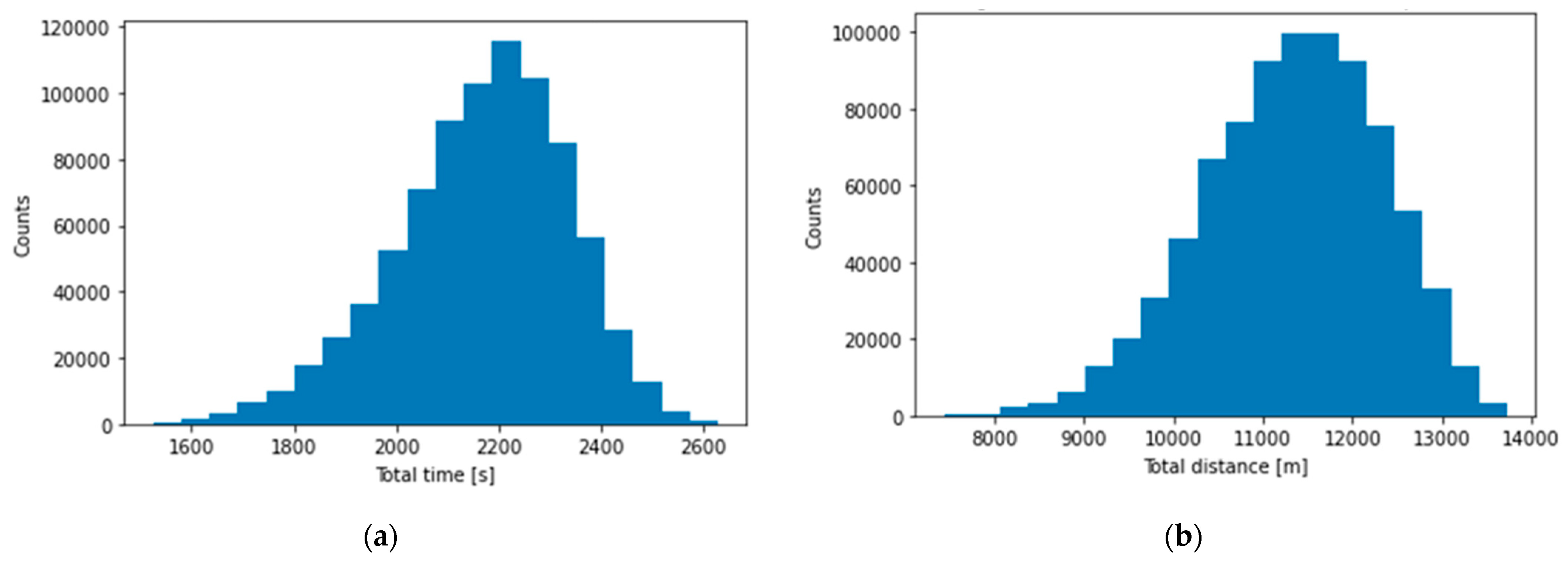
Using this approach all feasible solutions were achieved. Due to large number of permutations, only best routes according to time were taken into consideration. The histograms for all 2D feasible, time-optimal routes are shown on Figure 2.

All TSP-optimal routes for all knapsacks have a mean time of 2780 s, maximum spread is 855 s and standard deviation of population is 164 s.

All 2D feasible solutions count was 827,772. They were calculated in 565 s. There were 41,253,456 route permutations, which were calculated in 298 s. Total algorithm runtime was 864 s. Average time of all 2D feasible routes was 2168 s with population standard deviation of 168 s and range of 1105 s. Mean distance of all 2D feasible routes was 11,325 m with population standard deviation of 991 m and range of 6290 m.

This algorithm managed to find optimal route [[0, 0, 3, 5, 9], [0, 0, 6, 8], [0, 0, 2, 7, 10], [0, 0, 1, 4]] with total travel time of 1525 s and total travel distance of 7914 m. Distance of optimal solution was also the minimum of all feasible distances.

5.2. MTSP-First Results

After calculating possible MTSP routes, every route for every vehicle is verified for mass and cubic capacity feasibility and rejecting solutions that are not feasible.

Histograms of total times and distances for all generated routes is presented on Figure 3.

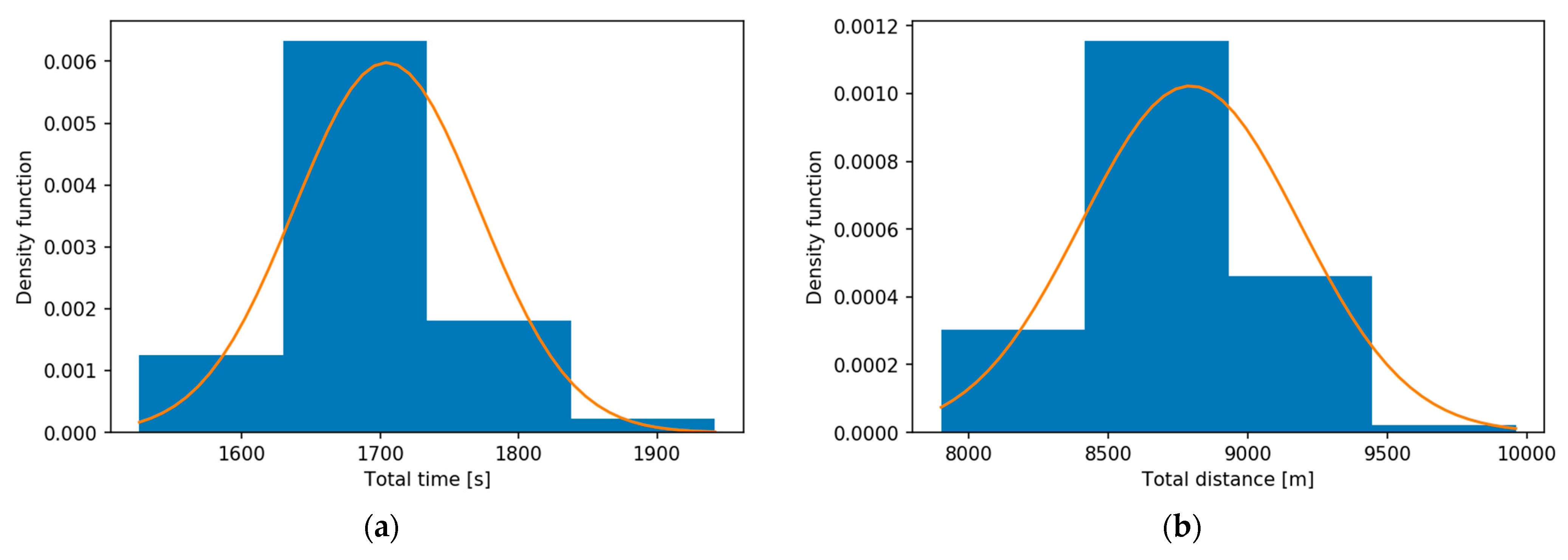
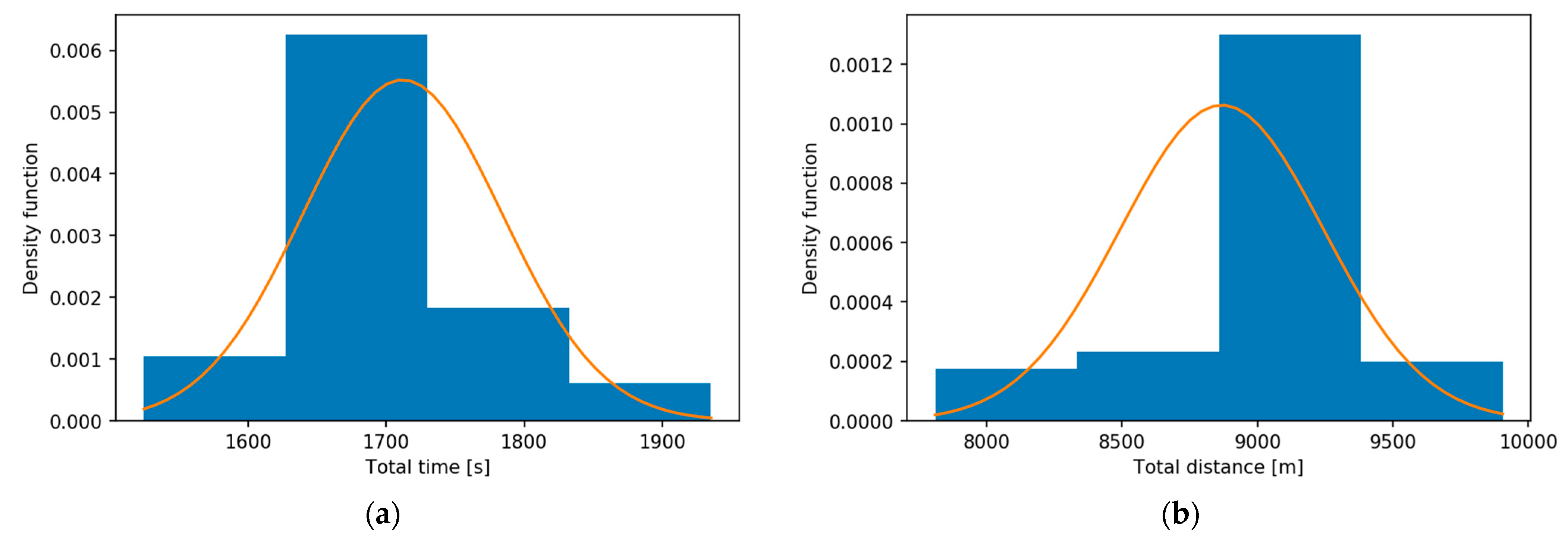
With MTSP solver being time-limited to 2 s total of 239 TSP solutions was found, 231 solutions were deemed feasible according to the weight and volume constraint. Total of 15 solutions were feasible according to packer algorithm thus being 3D feasible. 3D feasible routes histogram is shown on Figure 4.

Mean total time for all 3D feasible solutions was 1652 s, with population standard deviation of 88 s and spread between maximum and minimum time was 305 s. Mean distance for all those routes was 8376 m with population standard deviation of 392 m and spread between maximum and minimum distances was 1416 m. All given values were rounded to a full second or meter accordingly.

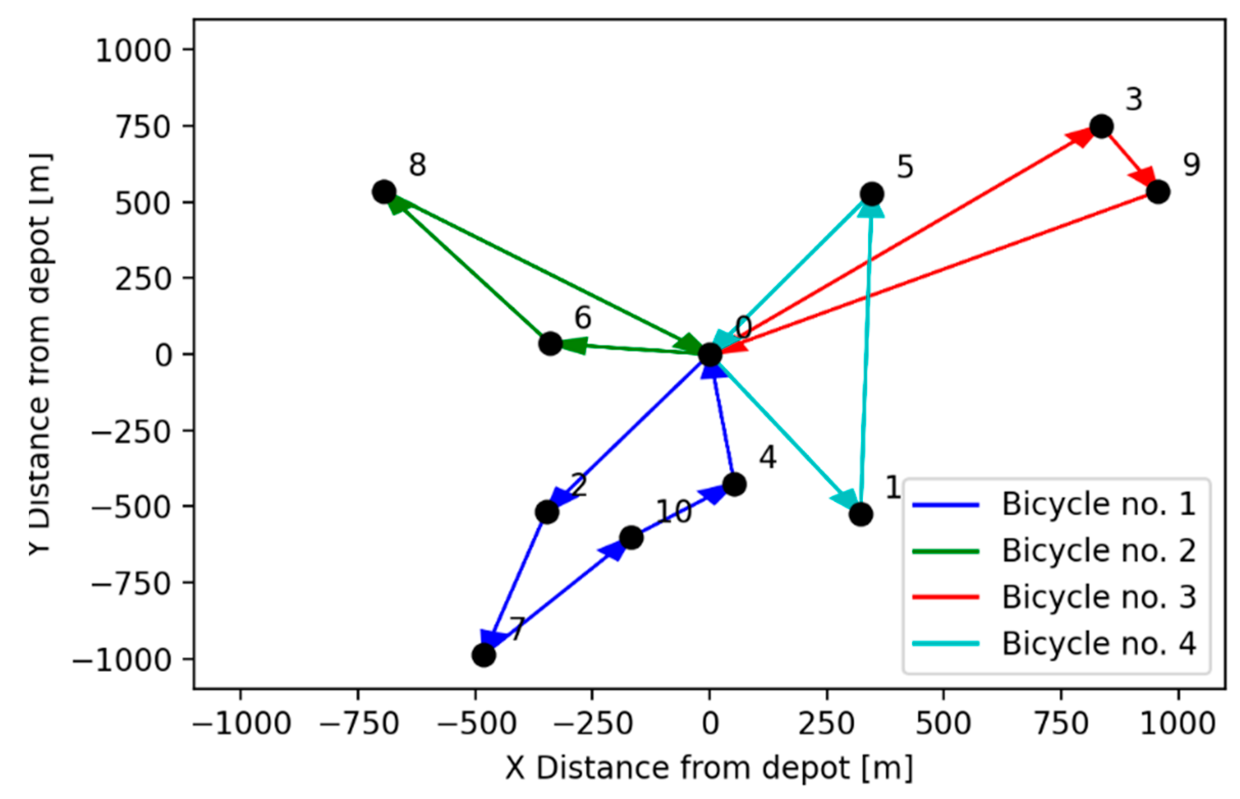
Best found route, according to total travel time using MTSP-First algorithm was [[0, 5, 3, 9, 0], [0, 6, 8, 0], [0, 10, 7, 2, 0], [0, 1, 4, 0]] with total time of 1526 s and total distance of 7913 m. This route is shown on Figure 5.

5.3. CVRP Approach Results

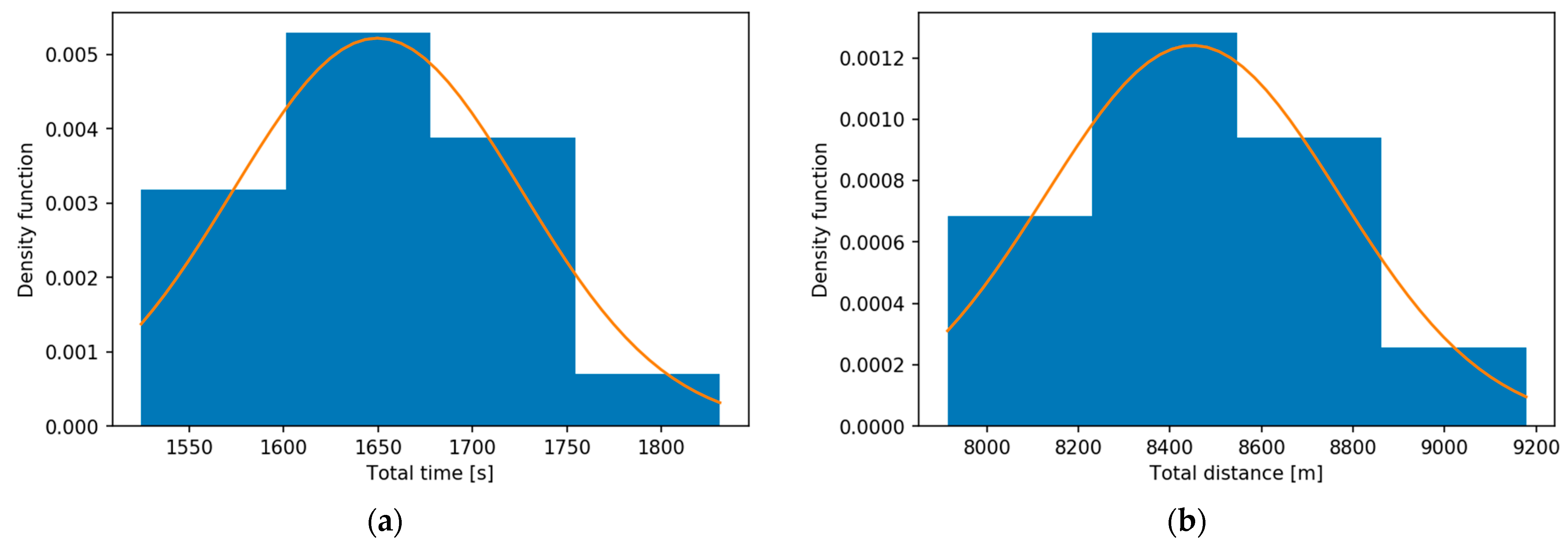
With CVRP solver runtime limited to 2 s it was able to generate 211 solutions, which were 2D feasible. Histograms of those values according to total travel time and distance are shown on Figure 6. 28 of those solutions were deemed 3D feasible.

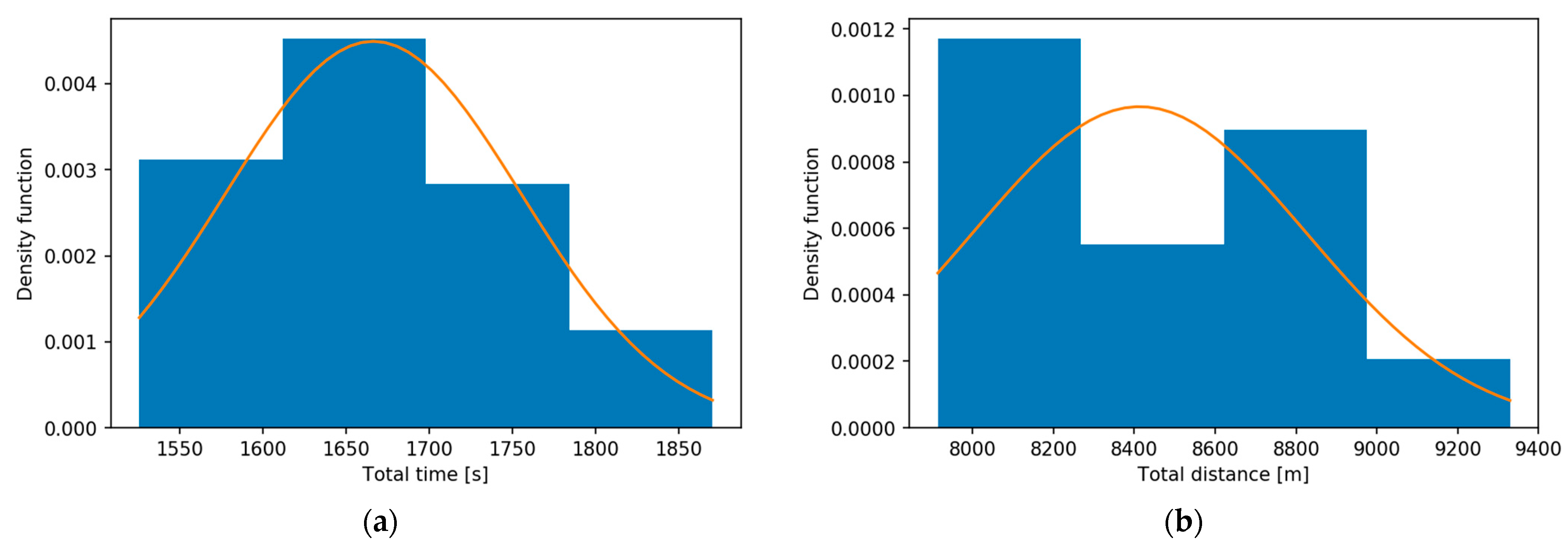
Best found route according to total travel time was [[0, 10, 7, 2, 0], [0, 6, 8, 0], [0, 5, 3, 9, 0], [0, 1, 4, 0]], with travel time of 1525 s and distance of 7 914 m. Average total travel time of all 3D feasible solutions was 1705 s with population standard deviation of 70 s and range of 411 s. Mean distance of all 3D feasible routes was 8817 m with population standard deviation of 398 m and difference between maximum and minimum values of 2095 m. Histograms representing those data are shown on Figure 7.

As can be seen on Figure 8 the bicycle routes with best total travel time had the same nodes as the route with minimum total travel distance, but the sequence of node visits was different.

5.4. Result Comparison

Results, achieved by metaheuristic methods (MTSP and CVRP) were similar to values calculated deterministically. The results are presented in

Table 3. Experiment results.

Parameters	Used Algorithm
	Bin Pack 3D	MTSP	CVRP
Total route time [s]	1525	1526	1525
Total route distance [m]	7914	7913	7914

.

As can be seen from the numbers in Table 3, for the synthetic dataset used in this research, the route parameters for the best solution generated by the corresponding algorithms are almost identical, although the shapes of the obtained routes differ insignificantly. Thus, the main criterion to choose the heuristic method is the time needed to achieve the result by running the corresponding algorithm: both proposed metaheuristics are characterized by the calculation time feasible under real-world conditions. However, the CVRP approach in contrast with the MSTP heuristics was able to find an optimal solution, which is why it will be used for further research under real-life applications.

6. Conclusions

In this work, we deal with a combination vehicle routing problem with 3D loading constraints and load-dependent time. This approach is similar to CVRP formulated by Dantzig and Ramser except for additional constraints, namely, speed being dependent on the load carried by a vehicle as into traveling thief problem. This research is given by the problem of last-mile delivery with the use of cargo bicycles, which are powered by the strength of human muscles thus low power so they cannot achieve high speeds and those speeds will be even lower when the bicycle is fully loaded. Two wheeled cargo bicycles have capacity lower to their three or four wheeled counterparts, but with the lighter load it would allow for faster deliveries, due to being less cumbersome to ride in densely populated urban areas and being less susceptible to traffic congestions.

We have achieved an optimal solution for a given dataset by deterministically calculating all possible knapsack combinations and calculating the best route according to the total travel time for each knapsack combination. This deterministic approach was used as a benchmark for comparing two metaheuristic approaches, the first being CVRP with total load and cubic capacity and 3D packing feasibility restrictions. The second approach was made as an MTSP approach with a check for feasibility according to mass, volume and 3D packing constraints. Testing of algorithms proved that the CVRP approach was able to produce optimal solutions in 2 s for 4 bicycles and 10 consignments, which concludes that this approach is better suited for real-life applications with dynamically appearing consignments and will be further investigated. MTSP approach was not able to produce an optimal solution.

Future work should enable implementing efficient 3D packing plans with LIFO constraints so that packages can be removed without moving other consignments. In addition, a constraint programming approach to the whole problem will be attempted with various metaheuristic approaches.

References

- United Nations, Department of Economic and Social Affairs. The World ’s Cities in 2018. In The World’s Cities in 2018—Data Booklet (ST/ESA/ SER.A/417); United Nations, Department of Economic and Social Affairs, Population Division: New York, NY, USA, 2018; p. 34. [Google Scholar]
- United Nations. World Population Prospects Key Findings & Advance Tables; ESA/P/WP.241; United Nations: New York, NY, USA, 2015. [Google Scholar]
- Ranieri, L.; Digiesi, S.; Silvestri, B.; Roccotelli, M. A Review of Last Mile Logistics Innovations in an Externalities Cost Reduction Vision. Sustainability 2018, 10, 782. [Google Scholar] [CrossRef] [Green Version]
- Taefi, T.T.; Kreutzfeldt, J.; Held, T.; Fink, A. Supporting the adoption of electric vehicles in urban road freight transport—A multi-criteria analysis of policy measures in Germany. Transp. Res. Part A Policy Pract. 2016, 91, 61–79. [Google Scholar] [CrossRef]
- Taefi, T.T.; Kreutzfeldt, J.; Held, T.; Konings, R.; Kotter, R.; Lilley, S.; Baster, H.; Green, N.; Laugesen, M.S.; Jacobsson, S.; et al. Comparative Analysis of European Examples of Freight Electric Vehicles Schemes—A Systematic Case Study Approach with Examples from Denmark, Germany, the Netherlands, Sweden and the UK. Optim. Decis. Support Syst. Supply Chains 2016, 495–504. [Google Scholar] [CrossRef] [Green Version]
- Taefi, T.T. Viability of electric vehicles in combined day and night delivery: A total cost of ownership example in Germany. Eur. J. Transp. Infrastruct. Res. 2016, 16, 512–553. [Google Scholar] [CrossRef]
- Elbert, R.; Friedrich, C.; Boltze, M.; Pfohl, H.-C. Urban Freight Transportation Systems: Current Trends and Prospects for the Future; Published in Cooperation with WCTRS; Elsevier BV: Amsterdam, The Netherlands, 2020; pp. 265–276. [Google Scholar]
- CIVITAS. Making urban freight logistics more sustainable. Civ. Policy Note 2015, 1–63. Available online: http://www.eltis.org/ (accessed on 4 June 2021).
- Anderluh, A.; Hemmelmayr, V.; Nolz, P.C. Sustainable Logistics with Cargo Bikes—Methods and Applications. Sustain. Transport. Smart Logist. 2019, 207–232. [Google Scholar] [CrossRef]
- Wrighton, S.; Reiter, K. CycleLogistics—Moving Europe Forward! Transp. Res. Procedia 2016, 12, 950–958. [Google Scholar] [CrossRef] [Green Version]
- Baum, L. Planning of Cargo Bike Hubs. A Guide for Municipalities and Industry for the Planning of Transshipment Hubs for New Urban Logistics Concepts. 2020. Available online: https://cyclelogistics.eu/sites/default/files/downloads/Hub%20Planning%20Brochure_EN_Web_final.pdf (accessed on 4 June 2021).
- Chiffi, C.; Reiter, K. Shared Micro-Hubs, Locker Systems and Cycle-Based Delivery Services for Achieving Zero Emission Urban Logistics. 2015. Available online: https://civitas.eu/sites/default/files/documents/cyclelogistics-civitas_final.pdf (accessed on 4 June 2021).
- Naumov, V.; Starczewski, J. Choosing the Localisation of Loading Points for the Cargo Bicycles System in the Krakow Old Town. In International Conference on Reliability and Statistics in Transportation and Communication; Lecture Notes in Networks and Systems; Springer Science and Business Media LLC: Cham, Switzerland, 2019; pp. 353–362. [Google Scholar]
- Enthoven, D.L.; Jargalsaikhan, B.; Roodbergen, K.J.; Broek, M.A.J.U.H.; Schrotenboer, A.H. The two-echelon vehicle routing problem with covering options: City logistics with cargo bikes and parcel lockers. Comput. Oper. Res. 2020, 118, 104919. [Google Scholar] [CrossRef]
- Lee, K.; Chae, J.; Kim, J. A Courier Service with Electric Bicycles in an Urban Area: The Case in Seoul. Sustainability 2019, 11, 1255. [Google Scholar] [CrossRef] [Green Version]
- Gruber, J.; Ehrler, V.; Lenz, B. Technical Potential and User Requirements for the Implementation of Electric Cargo Bikes in Courier Logistics Services. In Proceedings of the 13th World Conference on Transport Research (WCTR), Rio de Janeiro, Brazil, 15–18 July 2013; pp. 1–16. [Google Scholar]
- De Mello Bandeira, R.A.; Goes, G.V.; Gonçalves, D.N.S.; de Almeida D’Agosto, M.; De Oliveira, C.M. Electric vehicles in the last mile of urban freight transportation: A sustainability assessment of postal deliveries in Rio de Janeiro-Brazil. Transp. Res. Part D Transp. Environ. 2019, 67, 491–502. [Google Scholar] [CrossRef]
- Stamatiadis, N.; Pappalardo, G.; Cafiso, S. Use of technology to improve bicycle mobility in smart cities. In Proceedings of the 5th IEEE International Conference on Models and Technologies for Intelligent Transportation Systems, MT-ITS 2017, Naples, Italy, 26 June 2017; pp. 86–91. [Google Scholar]
- Gruber, J.; Narayanan, S. Travel Time Differences between Cargo Cycles and Cars in Commercial Transport Operations. Transp. Res. Rec. J. Transp. Res. Board 2019, 2673, 623–637. [Google Scholar] [CrossRef] [Green Version]
- Cheikhrouhou, O.; Khoufi, I. A comprehensive survey on the Multiple Traveling Salesman Problem: Applications, approaches and taxonomy. Comput. Sci. Rev. 2021, 40, 100369. [Google Scholar] [CrossRef]
- Dube, E.; Kanavathy, L.R. Optimizing Three-Dimensional Bin Packing Through Simulation. MSO. 2006. Available online: https://www.academia.edu/35965688/OPTIMIZING_THREE-DIMENSIONAL_BIN_PACKING_THROUGH_SIMULATION (accessed on 4 June 2021).
- Bonyadi, M.R.; Michalewicz, Z.; Barone, L. The travelling thief problem: The first step in the transition from theoretical problems to realistic problems. IEEE Congr. Evolut. Comput. 2013, 1037–1044. [Google Scholar] [CrossRef]
- Gruber, J.; Rudoph, C.; Lenz, B.P.; Liedtje, G.P.; Spath, C.; Wrighton, S. Untersuchung des Einsatzes von Fahrrädern im Wirtschaftsverkehr (WIV-RAD). 2016. Available online: https://elib.dlr.de/104273/1/WIV-RAD-Schlussbericht.pdf (accessed on 4 June 2021).
- Shaheen, A.; Sleit, A.; Al-Sharaeh, S. A solution for traveling salesman problem using grey wolf optimizer algorithm. J. Theor. Appl. Inf. Technol. 2018, 96, 6256–6266. [Google Scholar]
- Xu, J.; Pei, L.; Zhu, R.-Z. Application of a Genetic Algorithm with Random Crossover and Dynamic Mutation on the Travelling Salesman Problem. Procedia Comput. Sci. 2018, 131, 937–945. [Google Scholar] [CrossRef]
- Hacizade, U.; Kaya, I. GA Based Traveling Salesman Problem Solution and its Application to Transport Routes Optimization. IFAC PapersOnLine 2018, 51, 620–625. [Google Scholar] [CrossRef]
- Marinakis, Y.; Marinaki, M.; Dounias, G. A hybrid particle swarm optimization algorithm for the vehicle routing problem. Eng. Appl. Artif. Intell. 2010, 23, 463–472. [Google Scholar] [CrossRef]
- Tatavarthy, A.; Rao, T.S.; Marimuthu, K.P. A Simulated Annealing and Nearest Neighborhood Approach to Solve a Vehicle Routing Problem in a FMCG Company. Int. J. Mech. Prod. Eng. Res. Dev. 2018, 8, 349–354. [Google Scholar] [CrossRef]
- Mahi, M.; Baykan, O.K.; Kodaz, H. A new hybrid method based on Particle Swarm Optimization, Ant Colony Optimization and 3-Opt algorithms for Traveling Salesman Problem. Appl. Soft Comput. 2015, 30, 484–490. [Google Scholar] [CrossRef]
- Dantzig, G.B.; Ramser, J.H. The truck dispatching problem. Manag. Sci. 1959, 6, 80–91. [Google Scholar] [CrossRef]
- Gendreau, M.; Iori, M.; Laporte, G.; Martello, S. A Tabu Search Algorithm for a Routing and Container Loading Problem. Transp. Sci. 2006, 40, 342–350. [Google Scholar] [CrossRef]
- Ozbaygin, G.; Karasan, O.; Yaman, H. New exact solution approaches for the split delivery vehicle routing problem. EURO J. Comput. Optim. 2017, 6, 85–115. [Google Scholar] [CrossRef] [Green Version]
- Bortfeldt, A.; Yi, J. The Split Delivery Vehicle Routing Problem with three-dimensional loading constraints. Eur. J. Oper. Res. 2020, 282, 545–558. [Google Scholar] [CrossRef]
- Chen, Z.; Yang, M.; Guo, Y.; Liang, Y.; Ding, Y.; Wang, L. The Split Delivery Vehicle Routing Problem with Three-Dimensional Loading and Time Windows Constraints. Sustainability 2020, 12, 6987. [Google Scholar] [CrossRef]
- Li, X.; Zhao, Z.; Zhang, K. A Genetic Algorithm for the Three-Dimensional Bin Packing Problem with Heterogeneous Bins. 2014. Available online: https://www.researchgate.net/profile/Xueping-Li-4/publication/273121476_A_genetic_algorithm_for_the_three-dimensional_bin_packing_problem_with_heterogeneous_bins/links/54f742460cf2ccffe9dafbc2/A-genetic-algorithm-for-the-three-dimensional-bin-packing-problem-with-heterogeneous-bins.pdf (accessed on 4 June 2021).
- Perron, L.; Furnon, V. OR-Tools. 2019. Available online: https://developers.google.com/optimization (accessed on 4 June 2021).
Figure 1.
Node location and route with lowest total time.
Figure 2.
Histograms for all Bin Pack routes according to (a) time and (b) distance.
Figure 3.
Histograms for all MTSP routes according to time (a) and distance (b).
Figure 4.
Histograms for 3D feasible MTSP routes according to time (a) and distance (b).
Figure 5.
Route with best total travel time achieved from MTSP approach.
Figure 6.
Histograms for all CVRP routes according to time (a) and distance (b).
Figure 7.
Histograms for all 3D feasible CVRP routes according to time (a) and distance (b).
Figure 8.
Diagram representing route for calculated routes with lowest time (a) and distance (b).