
Health Assessment and Remaining Useful Life Prediction of Wind Turbine High-Speed Shaft Bearings

School of Electrical Engineering, Xinjiang University, Urumqi 830047, China
*
Author to whom correspondence should be addressed.
Energies 2021, 14(15), 4612; https://doi.org/10.3390/en14154612
Submission received: 15 May 2021
/
Revised: 7 July 2021
/
Accepted: 15 July 2021
/
Published: 30 July 2021
Abstract
:Vibration signals contain abundant information that reflects the health status of wind turbine high-speed shaft bearings ((HSSBs). Accurate health assessment and remaining useful life (RUL) prediction are the keys to the scientific maintenance of wind turbines. In this paper, a method based on the combination of a comprehensive evaluation function and a self-organizing feature map (SOM) network is proposed to construct a health indicator (HI) curve to characterizes the health state of HSSBs. Considering the difficulty in obtaining life cycle data of similar equipment in a short time, the exponential degradation model is selected as the degradation trajectory of HSSBs on the basis of the constructed HI curve, the Bayesian update model, and the expectation–maximization (EM) algorithm are used to predict the RUL of HSSBs. First, the time domain, frequency domain, and time–frequency domain degradation features of HSSBs are extracted. Second, a comprehensive evaluation function is constructed and used to select the degradation features with good performance. Third, the SOM network is used to fuse the selected degradation features to construct a one-dimensional HI curve. Finally, the exponential degradation model is selected as the degradation trajectory of HSSBs, and the Bayesian update and EM algorithm are used to predict the RUL of the HSSB. The monitoring data of a wind turbine HSSB in actual operation is used to validate the model. The HI curve constructed by the method in this paper can better reflect the degradation process of HSSBs. In terms of life prediction, the method in this paper has better prediction accuracy than the SVR model.
1. Introduction
Grid-connected wind turbines are required to operate in harsh environments for a long time. Due to long-term uninterrupted operation and the impact of extreme weather, rainfall, snowfall, etc., the health status and reliability of various wind turbine components will inevitably decline over time, eventually leading to failure. Studies have shown that the main sources of wind turbine failure include transmission shaft systems, gearboxes, generators, electrical control systems, and other key components. The maintenance cost of these faults will directly affect the economic benefits of wind farms [1]. According to surveys, the maintenance cost of onshore wind turbines with a design service life of 20 years accounts for about 15–20% of the total profit of the wind farm, while the maintenance cost of offshore wind turbines accounts for as much as 20–25% of the total profit [1,2]. As a key and vulnerable mechanical component of wind turbine transmission systems, high-speed shaft bearings (HSSBs) are of great practical significance for improving the safe operation of wind turbines and reducing wind farm operation and maintenance costs [3,4].
The health status assessment of equipment uses state monitoring data to model the performance degradation process, thereby constructing a one-dimensional health indicator (HI) curve to characterize the performance degradation process of the equipment [5]. As the running time increases, the health status of wind turbine HSSB is gradually degraded. The health assessment is a quantitative assessment of HSSB from an intact state to a series of different degradation states. The constructed HI curve should be able to accurately reflect the degradation process of the equipment in time. In recent years, researchers have focused on the assessment of equipment health status and achieved fruitful results. Reference [6] extracted time domain features from the vibration signal of rolling bearings and used monotonicity indicators to evaluate the degradation process of time domain features. Reference [7] used kurtosis to describe the degradation process of wind turbine HSSBs and applied this indicator to the prediction of the remaining life of HSSBs. The transmission structure of wind turbines is complex, a single feature cannot fully reflect the operating state of the HSSB in the transmission system, and a single time-domain or frequency-domain feature is easily affected by changes in operating conditions. Jin et al. [8] first calculated the energy values of the wavelet decomposition coefficient of the monitoring signal and fused them to construct an HI using the Mahalanobis distance between the energy values. Reference [9] used principal component analysis (PCA) for data fusion and constructs system health indicators using the first principal component with the largest variance. Jianbo Yu [10] extracted principal components from multiple features using dynamic PCA to construct the Mahalanobis distance based on the hidden Markov model and used the distance as an HI to reflect the equipment degradation process. If PCA is directly performed on all the extracted features, the first principal component after dimensionality reduction has a very low contribution rate, and the first principal component cannot accurately reflect the degradation trend of the equipment because some of these features contain a large amount of useless and redundant information that cannot be used to characterize the performance degradation and failure of the equipment. Reasonable selection of the degradation characteristics that can reflect the degradation state of equipment is the key to constructing an HI curve. Javed K et al. [11] used trigonometric functions and cumulative transformations for feature extraction, combined monotonicity, and trendability to screen the extracted features and fuse them to construct an HI curve. Zhang B et al. [12] constructed a feature evaluation function based on monotony, correlation, and robustness, and screened the extracted features accordingly. Finally, the moving average method was used to extract the selected degradation feature trends and construct HI curves. Reference [13] used an improved restricted Boltzmann machine to extract features from one-dimensional information and used the self-organizing mapping (SOM) network to integrate multiple features into the HI curve. Rai A et al. [14] used conventional signal processing techniques to extract multiple time-domain and frequency-domain features and used a SOM network to fuse the manually selected features into a one-dimensional HI curve. Due to the harsh operating environment and the complex transmission system of wind turbines, the vibration signals of each component are coupled and superimposed with each other. For these reasons, a comprehensive evaluation function is constructed to select excellent time domain, frequency domain, and time–frequency domain degradation features. The SOM network is used to fuse the selected degradation features and construct an HI curve to characterize the health status of wind turbine HSSBs.
In the field of equipment health management, a health index curve can be used for anomaly detection [15], fault prediction [16], etc. among which the remaining useful life (RUL) prediction of equipment is a key area of research [17,18,19]. The conventional RUL method is based on the full life cycle data of the equipment. However, in actual industrial fields, it is difficult to obtain the full life cycle data of a large amount of similar equipment in a short period of time. For expensive equipment such as wind turbines, the cost of obtaining the full life cycle data of key components is too high, and it is difficult to apply the conventional RUL prediction method based on full life cycle data to expensive equipment. Due to extreme environments and loads, the performance of the equipment will degrade with time and ultimately fail [20]. Therefore, establishing the degradation trajectory model by monitoring the equipment degradation data and predicting the RUL of the equipment is an economical and feasible method. Thus far, the exponential degradation model is one of the most popular degradation models [21]. In [22], an exponential stochastic model was used to describe the cumulative degradation process of bearings, and the Bayesian method was used to update the random parameters of the exponential degradation model and predict the RUL of bearings. Si X S et al. [23] used an exponential stochastic degradation model to model the cumulative degradation process of equipment and used the Bayesian update and expectation–maximization (EM) algorithm to estimate the model parameters and predict the RUL. Li N et al. [20] proposed an improved exponential stochastic degradation model to predict the RUL of rolling bearings. In [24], an exponential stochastic degradation model was used to model the life cycle of lithium batteries. In practice, it is often difficult to obtain sufficient historical degradation data for similar equipment, especially for newly operating equipment and expensive equipment. Considering these problems, this work uses the Bayesian update and expectation–maximization algorithm to predict the RUL of wind turbine HSSBs.
This work can be summarized into four steps: (1) extract the time domain, frequency domain, and time–frequency domain degradation characteristics of the vibration signal of the wind turbine HSSB; (2) use the comprehensive evaluation function constructed by monotonicity, correlation, and robustness to screen the degradation features; (3) use the SOM network to fuse the selected degradation features and construct the HI curve; (4) combine the Bayesian update and the expectation–maximization algorithm on the basis of the constructed HI curve to predict the RUL of the wind turbine HSSB.
2. Theoretical Methodology
2.1. Feature Evaluation Indicators
At present, the commonly used evaluation indicators for degradation include monotonicity, correlation, and robustness. The definition of each evaluation index is given below [12,25].
2.1.1. Monotonicity
The monotonicity index reflects the consistency degree of performance degradation between extracted features and equipment, namely, the intensity of a monotonically increasing or monotonically decreasing trend. The value range of this index is (0–1). The larger the monotonicity index is, the better the monotonicity trend of the features with the deterioration of equipment is. The monotonicity index is defined as follows:
where is the time series of the selected feature; represents the length of the selected feature; represents the differential of adjacent values in a sequence; and represent the counting values of the positive and negative derivatives, respectively.
2.1.2. Correlation
The correlation index reflects the degree of correlation between the extracted features and the equipment running time, and its value range is (0–1). The larger the correlation index is, the greater is the time correlation between the feature and equipment performance degradation; in other words, the degradation feature can better describe the equipment degradation process. The correlation index is defined as follows:
where is the time series of the selected feature, is the sample number, and is the sampling time series.
2.1.3. Robustness
The robustness index reflects the anti-interference ability of feature extraction, and its value range is (0–1). The larger the robustness index is, the smoother the variation rule of the feature with the degradation of equipment performance. This indicates that the uncertainty of the feature in the equipment performance degradation model and the prediction for the remaining life will be reduced.
where is the time series of the selected feature, and is the trend of the selected feature.
2.2. Minimum Quantization Error Based on SOM
2.2.1. SOM
SOM is a typical unsupervised competitive neural network [26]. The target output does not need to be given in advance and adaptive feature mapping can be performed according to the input data, which is very suitable for feature mapping and dimension reduction. The basic principle of SOM is to search and calculate the nearest neuron to the winning neuron according to Euclidean distance. The neuron with the minimum Euclidean distance is the winning neuron. The weights are adjusted according to the winning neuron. The specific implementation steps of the algorithm are as follows:
(1) The number of neurons in the topological layer is set as , and the maximum training time is . In general, the number of neurons in the topological layer is [27], and is the number of input samples;
(2) The network weights are randomly initialized;
(3) The input eigenvectors , a group of input samples are randomly selected , and the Euclidean distance between and the network weights is calculated, as shown in Equation (4)
where, is the weight vector between the i-th neuron in the input layer and the j-th neuron in the topology layer;
(4) Select the neuron with the minimum distance in as the best matching neuron, as shown in Equation (5)
where is the weight vector of the winning neuron , and updates its neighborhood neuron set at the same time;
(5) The inner star rule is used for weight learning, and the connection weight of the winning neuron c is updated and corrected, as shown in Equation (6)
where is the learning rate, , which decreases gradually with increasing training times;
(6) Training step , return to step (3) until the maximum number of training is reached, and is the weight vector of the best matching unit .
2.2.2. Minimum Quantization Error
In most cases, accurately collecting failure mode data is difficult, but obtaining data in the normal state is more convenient. Therefore, the quantization error deviating from the normal feature space can be used to describe the performance degradation process of equipment. First, the SOM is trained with data in the normal state, and the minimum quantization error is calculated by inputting the acquired measurement data into the SOM trained with normal data, which can be used as a new performance evaluation index. The distance between and the input data indicates that the input data deviates from the normal state, and therefore, the health index of the device equipment can be defined as follows [28]:
where MQE is the minimum quantization error, is the input eigenvector, and the health indicator is the health index curve of the equipment.
2.3. Degradation Model and Life Prediction
2.3.1. Degradation Modeling
The exponential degradation model is one of the most common methods used to describe the degradation process of components. At present, the exponential degradation model has been widely used in describing bearing wear, equipment corrosion, and other fields and has achieved good prediction results [21,22,24]. Let denote the degradation at a time ; then, the equipment adopts the exponential degradation model at the discrete-time monitoring point.
where is a fixed constant; and are random variables, and are used to describe the individual differences between different devices; is a random error term that obeys a Gaussian distribution . are independent and identically distributed random variables, and are independent of each other. Generally, logarithmic change is used to simplify the exponential degradation modeling process. After transforming Equation (8), Equation (9) can be obtained.
where , , and .
2.3.2. Stochastic Parameter Update of the Degradation Model Based on the Bayesian Method
Let and ; since are independent and identically distributed random variables, under the conditions of and , the conditional joint density function of the degenerate sample is
Since the prior distributions of and are Gaussian distributions, the posterior distributions of and still obey a Gaussian distribution under given conditions , [23]. Thus,
where
and are the mean values of the posterior estimate of and , , and are variances of the posterior estimate of and , and is the corresponding correlation coefficient.
2.3.3. RUL Prediction
To predict the RUL of the wind turbine HSSB, it is necessary to predict the future degradation trend of the equipment based on . When the degradation of HSSB exceeds the given failure threshold , the equipment will fail, and the useful life will end; therefore, the prediction of RUL is transformed into a predicted time when the degradation reaches the failure threshold . For the current time at through time , its logarithmic degradation is , can be proven to obey a Gaussian distribution [24], that is
where
Suppose the time interval from the current time to equipment failure is , that is, is the remaining useful life of the time . From the above definition of degradation failure and the logarithmic transformation characteristics of the degradation model, should satisfy . Then, for a given , the conditional cumulative distribution function of the RUL is
where , obeys a standard normal distribution, and is the cumulative distribution function of the standard normal distribution random variables. Since represents the RUL of the moment , is a non-negative real number, namely, . The RUL conditional cumulative distribution function is truncated under the condition of , and the following estimation results are obtained:
Then, the conditional probability density function of the corresponding RUL is
where is the probability density function of standard normal distribution random variables.
Equations (20) and (21) are the conditional cumulative distribution function and conditional probability density function of the RUL, respectively. It is difficult to calculate the RUL directly through Equations (20) and (21). According to the previous definition of degradation failure and the logarithmic transformation characteristics of the degradation model, we can obtain . The mean value of the predicted degradation is replaced with , and we can obtain . The approximate estimated value of the RUL at moment under the maximum probability is [25]
where and can be calculated according to Equations (12) and (13), but , , , , and are unknown in Equations (12) and (13). The abovementioned unknown parameters can be estimated using the maximum expectation algorithm.
2.3.4. Parameter Estimation Based on EM Algorithm
Reference [22] used the EM algorithm to estimate the parameter vector of five unknown parameters. Based on the method of maximum likelihood estimation, after obtaining the monitoring data at time , the logarithmic likelihood function of is calculated as follows:
where represents the joint probability density function of the degraded data, and therefore, the of maximum likelihood estimation at moment is
where is the value of the parameter vector corresponding to the maximum value, i.e., .
Using the Bayesian method and EM method, the estimation method of can be implemented through the following iterative process.
- (1)
- Calculatewhere represents the latest value of the ith iteration.
- (2)
- Calculate .
Usually, when the difference between and is less than a relatively small value, the iteration is terminated, and the result of the final estimation is taken as the final parameter estimation result at time [29]. Then, the EM algorithm is used to estimate the unknown parameters. For all the degradation monitoring data up to the time , the unknown estimation parameters are expressed as
The results of the ith iteration under the maximum expectation algorithm are as follows:
Then, the complete log-likelihood function can be expressed as
From Equations (25) and (28), we can obtain
Let , and we can obtain the parameter estimation of step . References [22,29] show that this is the only solution of .
Among which
The abovementioned parameter estimation method is an iterative process to estimate unknown parameters based on the degradation data to time . The iteration termination condition is that when the norm of the difference between the parameter vectors of the two iterations is less than a certain threshold, the iteration will be stopped, and the last is taken as the parameter used to calculate the RUL at time .
3. Plan Steps
3.1. Construct Comprehensive Evaluation Function
To select features with excellent performance, the above monotonicity, correlation, and robustness should be considered comprehensively [12]. A linear combination equation is established, and the features with larger weights are selected as sensitive features for constructing the HI curve and RUL prediction through multiobjective optimization. The linear combination is established as follows:
where is the comprehensive evaluation function of multiobjective optimization and are the weights of the three evaluation indexes. can be used as a comprehensive evaluation function to extract features by weighted fusion. The larger the of a certain feature is, the better the overall performance of the feature, which can better describe the degradation process of equipment performance.
3.2. Construct HI Curve
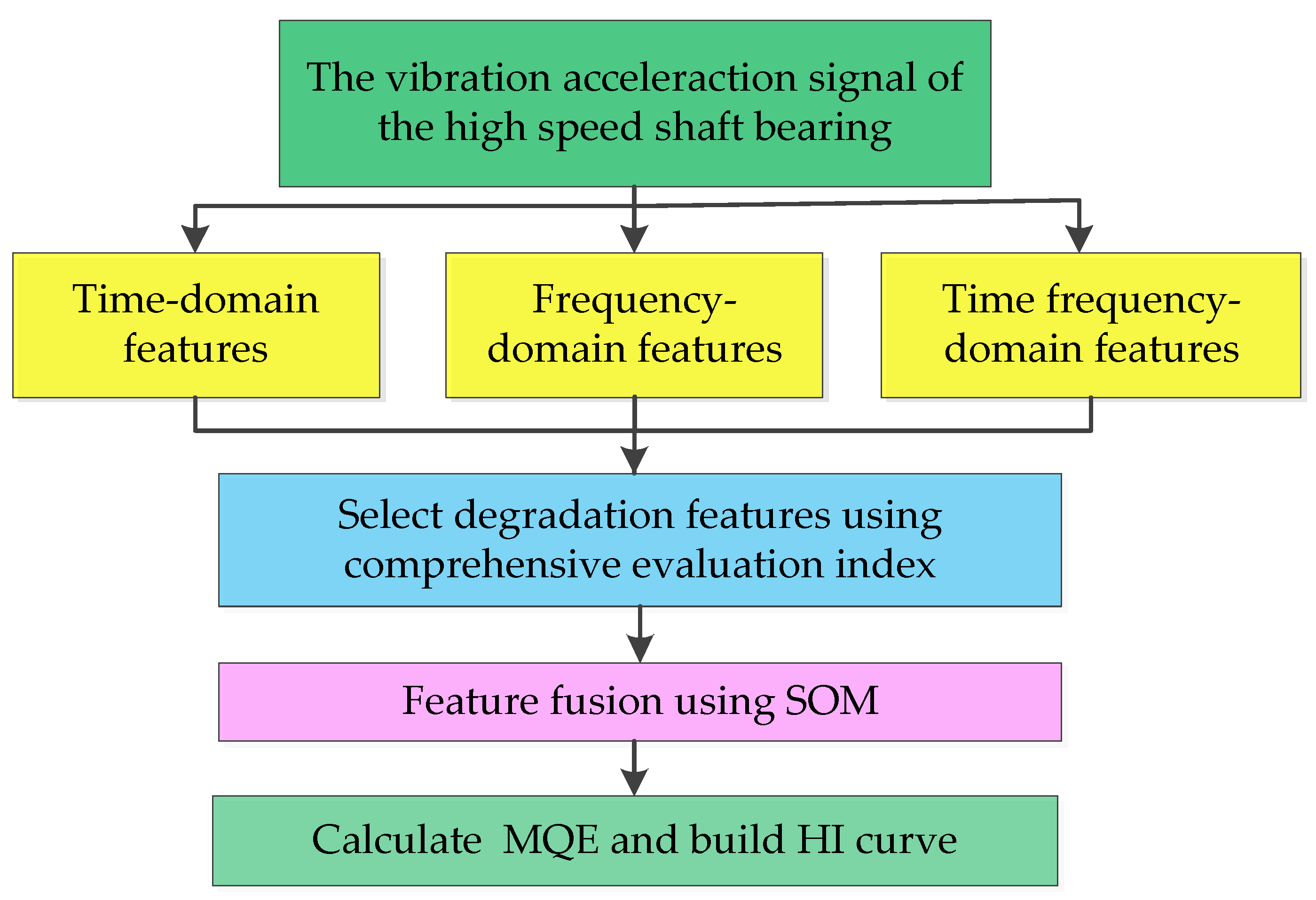
To evaluate the health status of a wind turbine HSSB, the HI curve is constructed using a comprehensive feature evaluation function and SOM. The flow chart used to construct the HI curve is shown in Figure 1 below.
The specific steps are as follows:
- Collect acceleration vibration signals of wind turbine HSSB;
- Extract degradation features of the vibration signal in the time, frequency, and time–frequency domain;
- Construct a comprehensive evaluation function considering monotonicity, correlation, and robustness and use the comprehensive evaluation function to select degradation features with excellent performance;
- Use SOM to fuse the selected degradation features;
- Calculate the minimum quantization error and construct the HI curve.
3.3. Use Exponential Degradation Model to Predict the RUL of HSSB
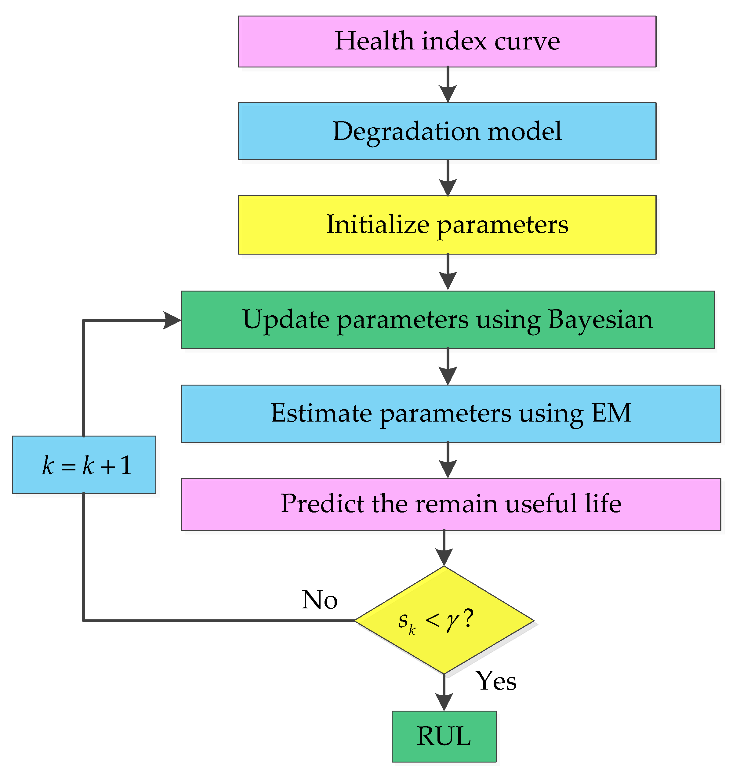
Based on the constructed health index curve, an exponential degradation model is selected to describe the degradation process of high-speed shaft bearings in wind turbines. The Bayesian update and expectation–maximization algorithm are combined to calculate the parameters of the exponential degradation model and predict the remaining life of the high-speed shaft bearings. The flow chart of the exponential degradation model is shown in Figure 2 below.
The specific steps are as follows:
- Select the exponential degradation model according to the constructed health index curve;
- Initialize the degradation model parameters;
- Utilize the method combining Bayesian update and expectation–maximization algorithm to update and estimate the exponential degradation model parameters;
- Predict the RUL of high-speed shaft bearings.
4. Data Analysis
4.1. Data Sets
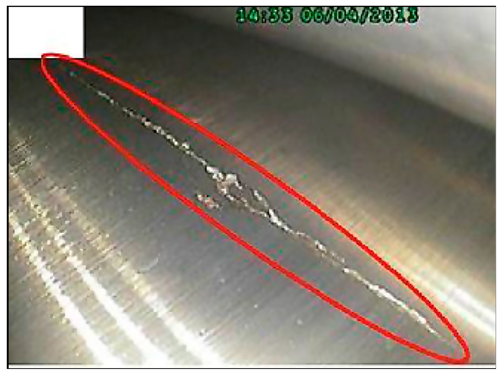
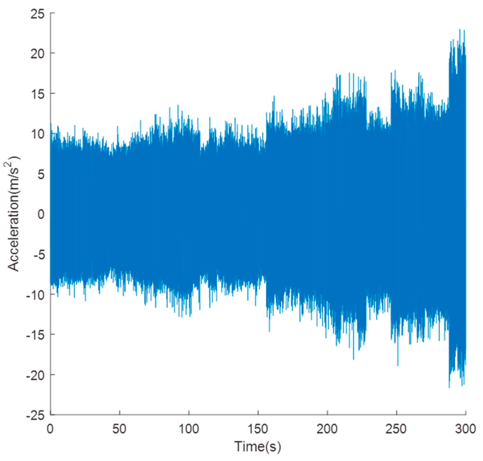
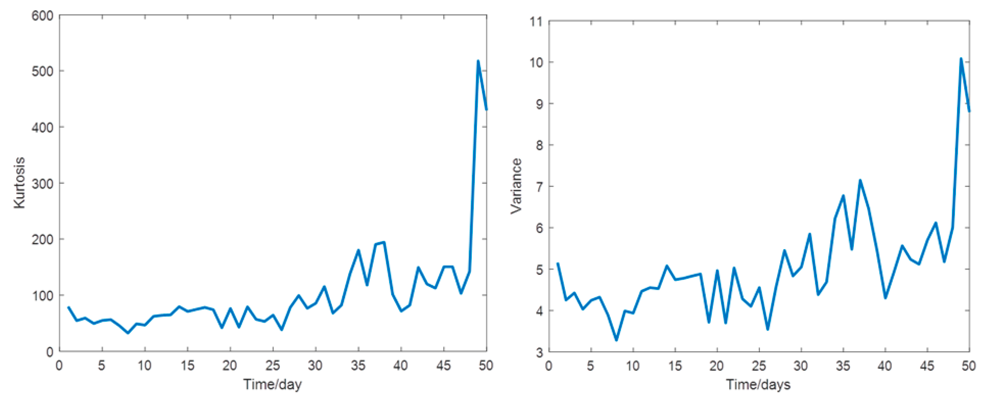
The HSSB test data in this work are from a real wind turbine provided by the US Green Power Monitoring System [7,30]. The wind turbine is 2.2 MW, and the vibration data are continuously sampled for 50 days. Each sample is 6 s, and the sampling frequency is 97,656 Hz. The sensor is installed radially on the high-speed shaft, the HSSB is supported by the gearbox bearing, and the sensor measures the vibration signal perpendicular to the shaft. The bearing model is a 32222-J2-SKF tapered roller bearing, which has 20 rolling elements, 16 degrees taper, and weighs approximately 20 pounds. The bearing was running at approximately 30 Hz, and on the last day, there was an inner race fault during the inspection. The HSSB test set is shown in Figure 3. As the recording time of vibration signals was 6 s per day for 50 days, the raw run-to-failure history of the tested bearing is shown in Figure 4. The time-domain features based on Table 1 provide 50 values of each feature where Figure 5 presents the evolution of some from the healthy bearing state to the failure state.
4.2. Extract Degradation Features
Due to the complex structure of the wind turbine transmission system, the harsh operating environment, and the superposition and mutual coupling of vibration signals of various components, a single feature cannot fully reflect the operating state of the wind turbine HSSB. Therefore, for 50 consecutive days of data, 36 features in the time domain, frequency domain, and time-frequency domain for each day of sampled data are extracted to reflect the operating status of the HSSB as comprehensively as possible [30,31].
4.2.1. Time Domain Features
The time-domain features directly calculate statistics on the vibration signal time series, which reflects the amplitude distribution and energy of the vibration signal. Let be the vibration signal sequence, n = 1, 2, …, N, where N is the number of samples. The time-domain feature calculation formula is shown in Table 1.
4.2.2. Frequency-Domain Features
The frequency-domain feature is the calculation of statistics on the frequency and amplitude of the frequency spectrum after the signal is transformed by FFT. The frequency spectrum of the signal after FFT transformation is (k = 1, 2, …, K), K is the number of spectral lines, and is the frequency value of the k-th spectral line. The frequency-domain feature calculation formula is shown in Table 2.
4.2.3. Time–Frequency Domain Features
Compared with ensemble empirical mode decomposition (EEMD), complementary ensemble empirical mode decomposition (CEEMD) has almost zero reconstruction error and can be used to solve the problem of different numbers of modes realized by different signals plus noise [32]. Entropy is a description of the degree of system uncertainty [33]. The more uncertain the information in the system is, the larger the corresponding entropy value is. Therefore, CEEMD decomposition and entropy can be combined to make use of their advantages and achieve impact signal analysis. The intrinsic mode function (IMF) energy entropy can reflect the change in amplitude energy in each frequency band of the signal, and therefore, this paper chooses to extract the IMF energy entropy as the time–frequency domain features of the vibration signal. The detailed calculation process of the CEEMD method is described in [32,34], which will not be repeated here. The calculation steps of IMF energy entropy are as follows:
The vibration signals of the wind turbine HSSB are decomposed by CEEMD, and the sum of a group of IMF components and residual terms are obtained [35,36,37]. The first n IMF energies are calculated as follows:
where is the number of IMF component data points, and is the amplitude of each point in the i-th IMF component.
The total energy of the first N IMF components is calculated as
The proportion of IMF components of each order is
From this, the energy entropy of IMF is
According to the above calculation process, the first 7 IMF energy entropies are selected as the time–frequency domain features.
4.3. Select Degradation Features
Since some of the extracted degradation features contain much useless information that cannot characterize the performance degradation and failure of HSSB, some features cannot be used for degradation assessment, HI construction, and RUL prediction. Therefore, the degradation features must be effectively selected.
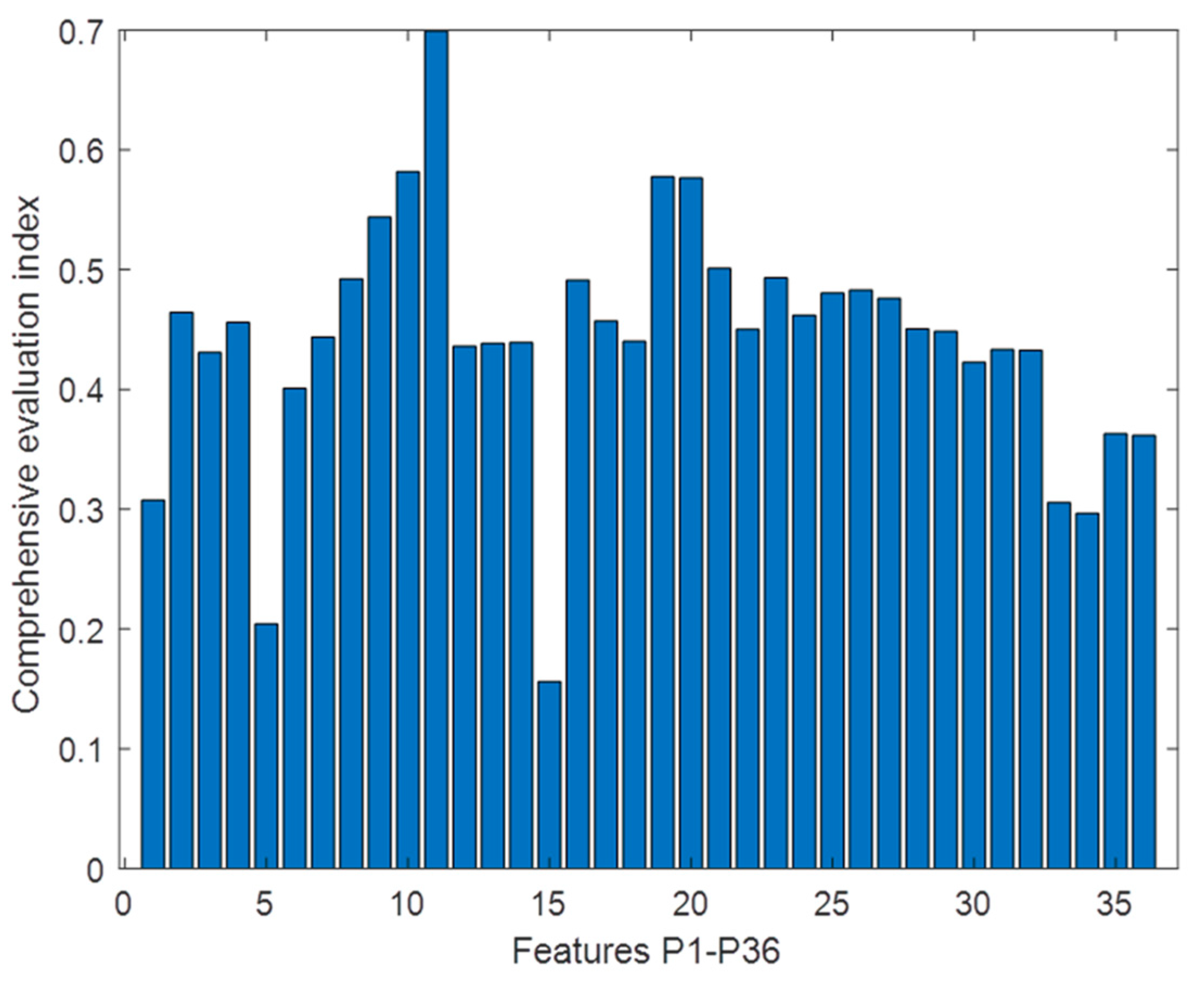
Monotonicity is more important when modeling the degradation process. Therefore, for Equation (30), the weights assigned to monotonicity, correlation, and robustness allocation are , , and . With the addition of the weights into Equation (30), the comprehensive evaluation values of each feature are shown in Figure 6. A histogram, that can be used to show the comprehensive evaluation index of each degradation feature more intuitively.
Select the features of the comprehensive evaluation index . The final selected degradation features are , , , , , , , , , , , , , , , , , , for a total of 18-dimensional features.
4.4. Construct HI Curve
After the degraded features are selected, multiple degraded features must be fused into a curve that can reflect the degradation state. In this paper, the SOM algorithm, combined with the minimum quantization error, is used to perform unsupervised feature fusion for the selected degradation features.
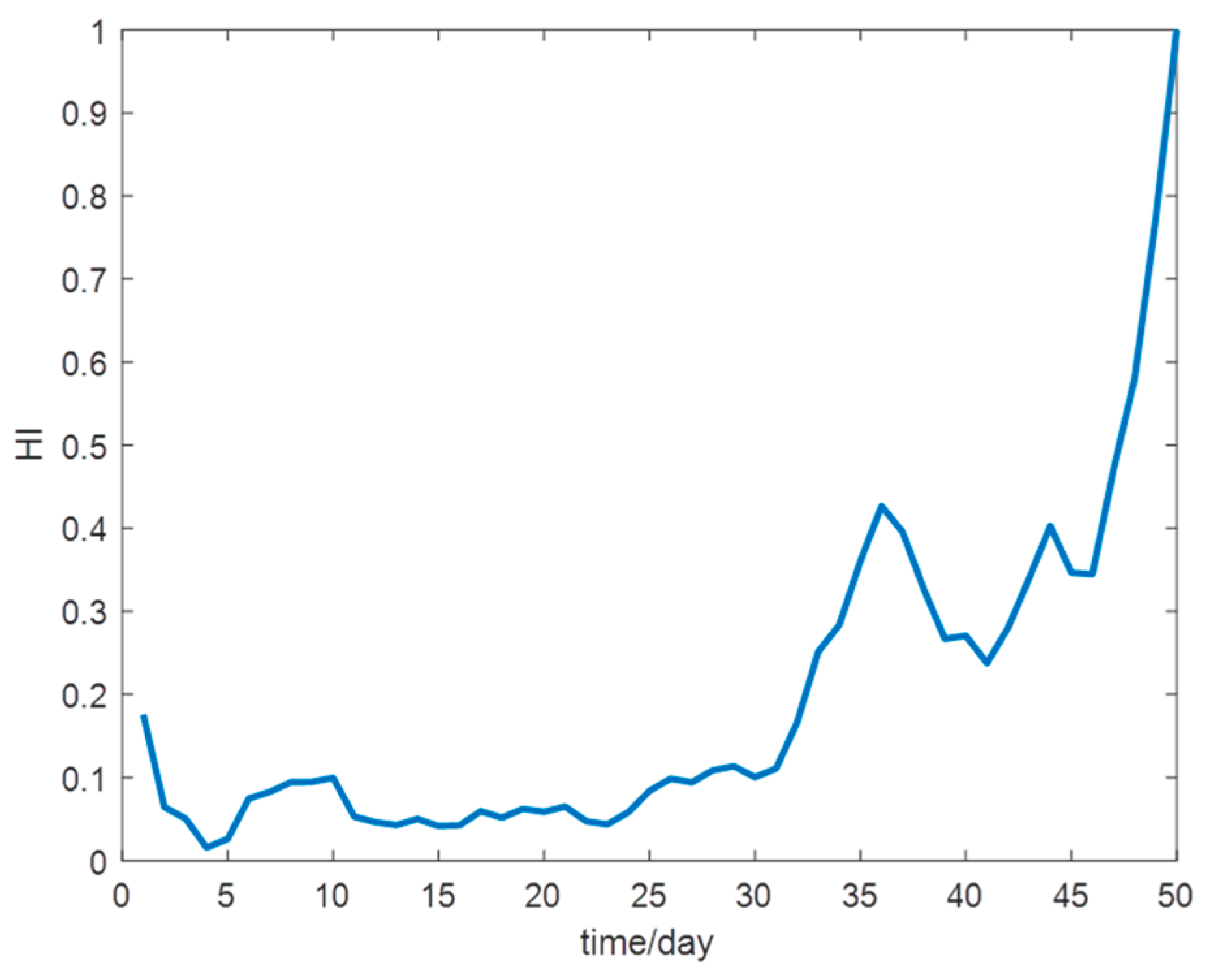
The number of nodes in the input layer of the SOM network is 18, which is consistent with the degradation feature dimension; the number of neurons is , and the number of feature iterations is 500. The normal state data of the first 5 days are selected to obtain the weight vector of the best winning unit. Then, according to Equation (7), the distance between the degradation characteristic data of 50 days and the best winning unit is calculated, which represents the HI of HSSB every day, and the distance quantitatively describes the performance degradation of bearings. The curve is processed by a moving average with a window size of 5 to reduce local noise, and the results are normalized and shown in Figure 7.
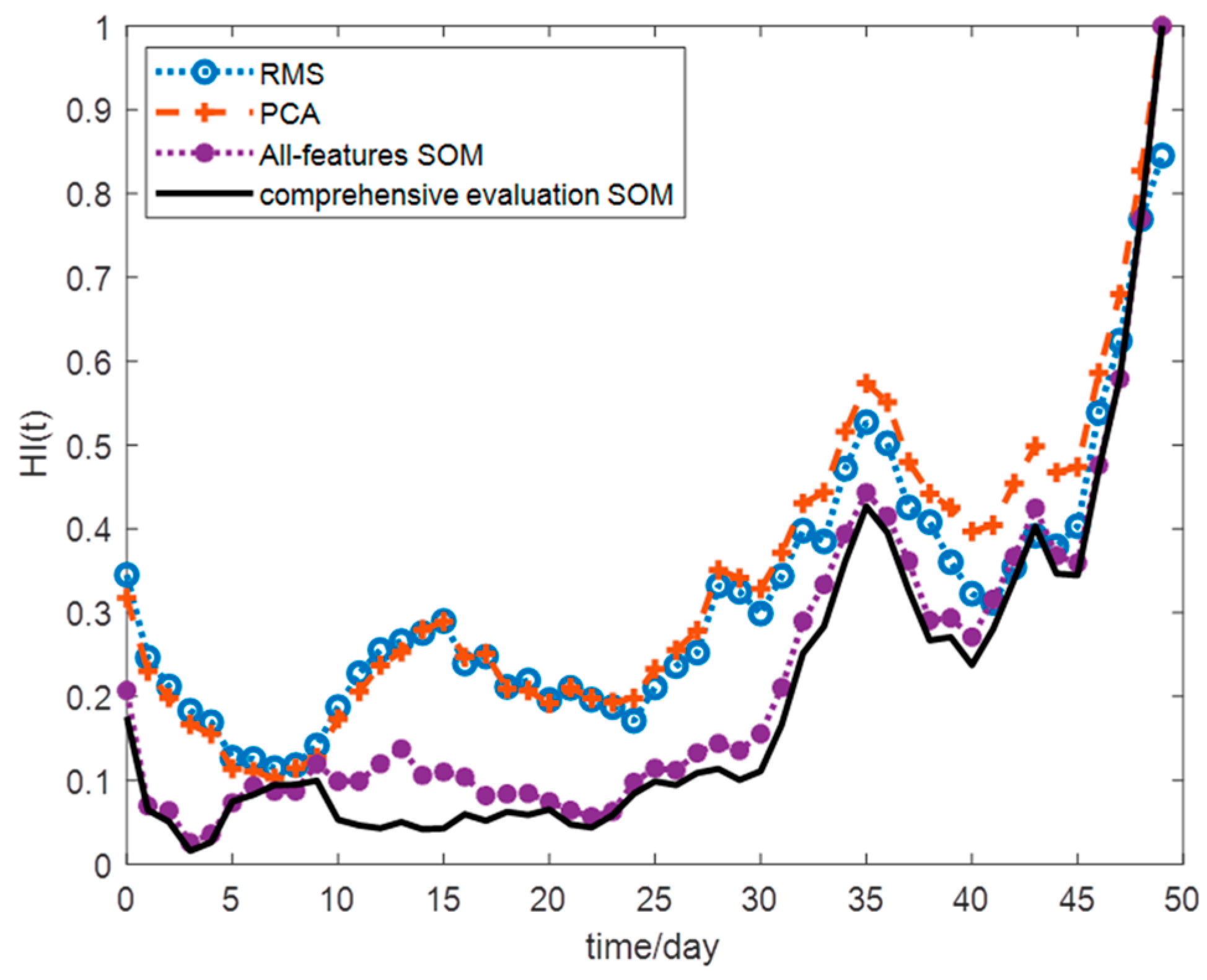
To verify the advantages of this method, RMS, PCA, and the HI curves constructed by SOM network fusion of all degradation features are used for comparative analysis. These curves are processed using a moving average with a window size of 5. The HI curve is constructed by the method in this paper, and the abovementioned comparison algorithm is shown in Figure 8. Obviously, the resulting HI curve is smoother and has better monotonicity and trend. The HI curve constructed by the method in this paper is an exponential function curve, and hence, the HI curve can be described by the exponential degradation model.
4.5. Using an Exponential Degradation Model to Predict the RUL of HSSB
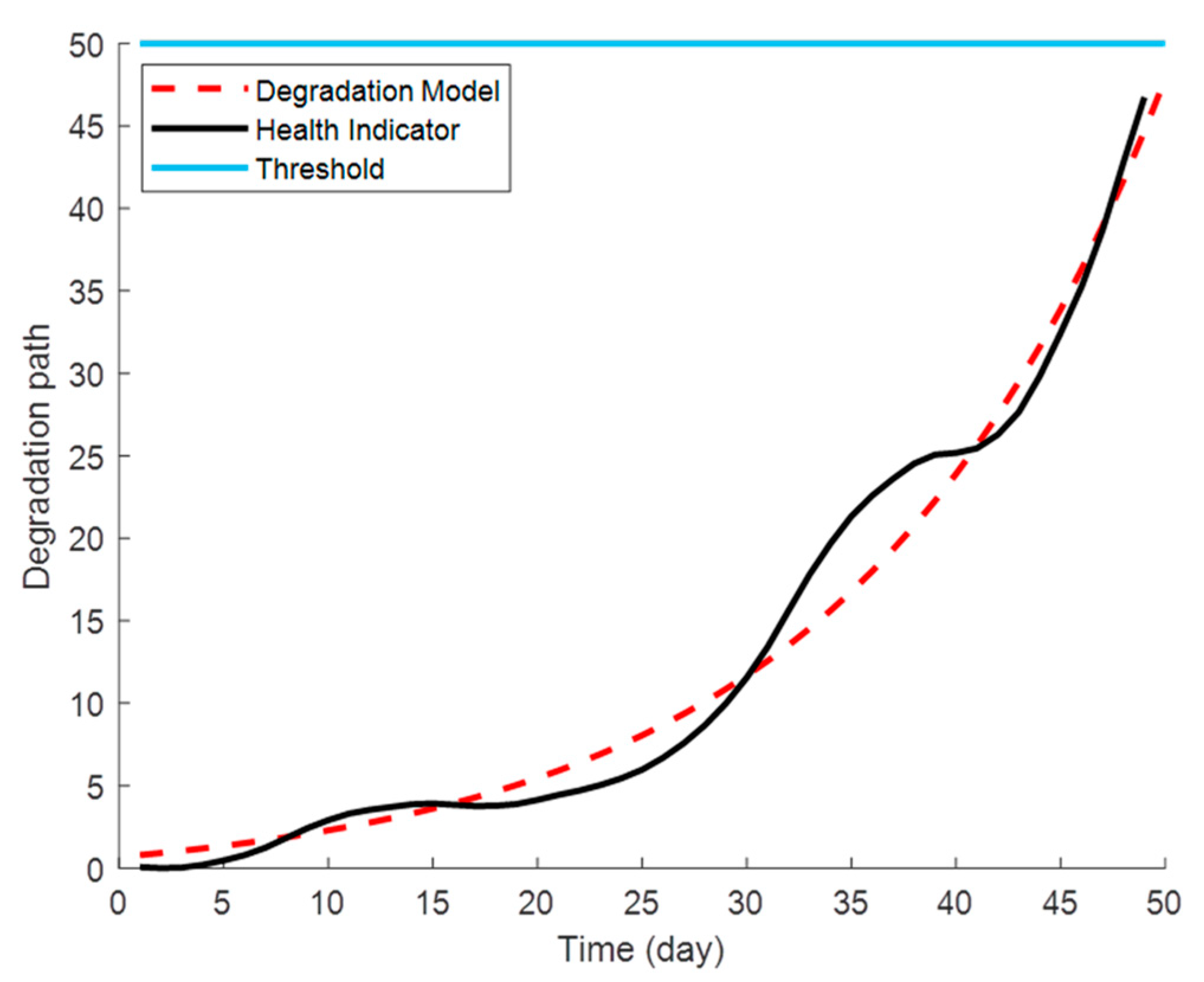
To eliminate the influence of burrs on the model parameters, db5 wavelet packet decomposition is used to decompose the HI curve constructed above. Equation (8) is selected as the exponential degradation model. Let the parameters of the model be , , , , and . The failure threshold is the HI value of the high-speed shaft bearing on the last day, namely, . The data of the first 30 days are selected to train and modify the parameters of the degradation model, and the parameters of the modified degradation model are , , , , and . Based on this, the actual degradation trajectory of the wind turbine HSSB and the degradation trajectory predicted by the exponential degradation model are shown in Figure 9.
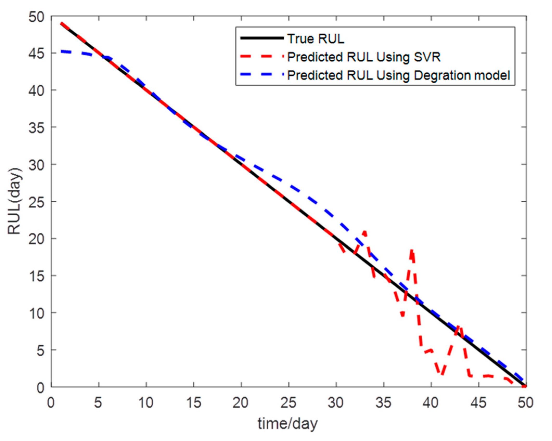
The point estimation of the RUL mentioned in this paper can be obtained through Equation (22). After the prediction is made, the parameters of the exponential degradation model are adjusted to , , , , and . Figure 10 shows the prediction results of the HSSB’s RUL using the method in this paper and the method in [7].
4.6. Evaluation Index
To analyze the effectiveness and accuracy of the prediction results of HSSB with the method in this paper and [7], the mean absolute error (MAE) [38] and root mean square error (RMSE) [39] are used as evaluation indexes for the prediction results of the two methods. According to these two indexes, the absolute error and relative error of each prediction result can be calculated. The calculation formulas are as follows:
where is the observed value; is the predicted value; N is the number of samples.
5. Conclusions
In this paper, a method combining a comprehensive evaluation function and a self-organizing neural network is proposed to construct an HI curve to evaluate the health status of wind turbine HSSBs. The method also uses an exponential degradation model to predict the RUL of the HSSB. This work can provide a theoretical basis for the subsequent maintenance plan of wind turbines.
- For the extracted high-dimensional degradation features, the comprehensive evaluation function can be used to eliminate features that do not reflect the degradation process of the wind turbine HSSB and that cannot reflect the degradation process effectively.
- It is difficult to reflect the degradation trend of wind turbine HSSB with a single time-frequency degradation feature. The HI curve generated by fusing the selected degradation features with the SOM algorithm can more accurately reflect the health status of HSSB.
- For the wind turbine HSSB, which lacks similar life cycle degradation data, the exponential degradation model based on the Bayesian update and expectation–maximization algorithm has degradation model parameters that will continue to update and continuous improvement of RUL prediction accuracy with the continuous accumulation of historical operation data.
This work has significance for the health assessment and RUL prediction of wind turbine HSSBs and provides scientific and reasonable support for subsequent maintenance plans.
Author Contributions
Conceptualization, Z.L. and X.Z.; methodology, Z.L.; software, Z.L.; validation, Z.L., X.Z. and W.H.; formal analysis, X.Z.; investigation, T.K.; resources, Z.L.; data curation, Z.L.; writing—original draft preparation, Z.L.; writing—review and editing, X.Z.; visualization, W.H.; supervision, X.Z.; project administration, X.Z.; funding acquisition, T.K. All authors have read and agreed to the published version of the manuscript.
Funding
This work was supported by the excellent youth scientific and technological talents plan of Xinjiang, China (Grant No. 2019Q012) and the Natural Science Foundation of autonomous region joint fund project, China (Grant No. 2021D01C044).
Institutional Review Board Statement
Not applicable.
Informed Consent Statement
Not applicable.
Data Availability Statement
HSSB data: https://www.mathworks.com/help/predmaint/ug/wind-turbine-high-speed-bearing-prognosis.html (accessed on 21 July 2021).
Conflicts of Interest
The authors declare no conflict of interest.
References
- Nie, M.Y.; Wang, L. Review of condition monitoring and fault diagnosis technologies for wind turbine gearbox. Procedia CIRP 2013, 11, 287–290. [Google Scholar] [CrossRef] [Green Version]
- Martinez-Luengo, M.; Kolios, A.; Wang, L. Structural health monitoring of offshore wind turbines: A review through the Statistical Pattern Recognition Paradigm. Renew. Sustain. Energy Rev. 2016, 64, 91–105. [Google Scholar] [CrossRef] [Green Version]
- Wiese, B.; Pedersen, N.L.; Nadimi, E.S.; Herp, J. Estimating the Remaining Power Generation of Wind Turbines—An Exploratory Study for Main Bearing Failures. Energies 2020, 13, 3406. [Google Scholar] [CrossRef]
- Dávila, Á.; Puruncajas, B.; Tutivén, C.; Vidal, Y. Wind Turbine Main Bearing Fault Prognosis Based Solely on SCADA Data. Sensors 2021, 21, 1–22. [Google Scholar]
- Lei, Y.G.; Li, N.P.; Guo, L.; Li, N.B.; Yan, T.; Jing, L. Machinery health prognostics: A systematic review from data acquisition to RUL prediction. Mech. Syst. Signal. Process. 2018, 104, 799–834. [Google Scholar] [CrossRef]
- Camci, F.; Medjaher, K.; Zerhouni, N.; Nectoux, P. Feature Evaluation for Effective Bearing Prognostics. Qual. Reliab. Eng. Int. 2013, 29, 477–486. [Google Scholar] [CrossRef] [Green Version]
- Saidi, L.; Ali, J.B.; Bechhoefer, E.; Benbouzid, M. Wind turbine high-speed shaft bearings health prognosis through a spectral Kurtosis-derived indices and SVR. Appl. Acoust. 2017, 120, 1–8. [Google Scholar] [CrossRef]
- Jin, X.H.; Sun, Y.; Que, Z.J.; Wang, Y.; Chow, W.S.T. Anomaly Detection and Fault Prognosis for Bearings. IEEE Trans. Instrum. Meas. 2016, 65, 2046–2054. [Google Scholar] [CrossRef]
- Zhao, S.K.; Jiang, C.; Long, X.Y. A residual life prediction method for mechanical systems based on data driven and Bayesian theory. J. Mech. Eng. 2018, 54, 115–124. [Google Scholar] [CrossRef]
- Yu, J.B. Health Condition Monitoring of Machines Based on Hidden Markov Model and Contribution Analysis. IEEE Trans. Instrum. Meas. 2012, 61, 2200–2211. [Google Scholar] [CrossRef]
- Javed, K.; Gouriveau, R.; Zerhouni, N.; Nectoux, P. Enabling Health Monitoring Approach Based on Vibration Data for Accurate Prognostics. IEEE Trans. Ind. Electron. 2015, 62, 647–656. [Google Scholar] [CrossRef] [Green Version]
- Zhang, B.; Zhang, L.J.; Xu, J.W. Degradation Feature Selection for Remaining Useful Life Prediction of Rolling Element Bearings. Qual. Reliab. Eng. Int. 2016, 32, 547–554. [Google Scholar] [CrossRef]
- Liao, L.X.; Jin, W.J.; Pavel, R. Enhanced Restricted Boltzmann Machine with Prognosability Regularization for Prognostics and Health Assessment. IEEE Trans. Ind. Electron. 2016, 63, 7076–7083. [Google Scholar] [CrossRef]
- Rai, A.; Upadhyay, S.H. Intelligent bearing performance degradation assessment and remaining useful life prediction based on self-organising map and support vector regression. J. Mech. Eng. Sci. 2017, 1–15. [Google Scholar] [CrossRef]
- Kudela, P.; Radzienski, M.; Ostachowicz, W.; Yang, Z.B. Structural Health Monitoring system based on a concept of Lamb wave focusing by the piezoelectric array. Mech. Syst. Signal. Process. 2018, 108, 21–32. [Google Scholar] [CrossRef]
- Shi, J.M.; Li, Y.X.; Wang, G.; Li, X.Z. Health index synthetization and remaining useful life estimation for turbofan engines based on run-to-failure datasets. Eksploat. I Niezawodn. Maint. Reliab. 2016, 18, 621–631. [Google Scholar] [CrossRef]
- Tian, Q.; Wang, H. An Ensemble Learning and RUL Prediction Method Based on Bearings Degradation Indicator Construction. Appl. Sci. 2020, 10, 346. [Google Scholar] [CrossRef] [Green Version]
- Berghout, T.; Benbouzid, M.; Mouss, H. Leveraging Label Information in a Knowledge-Driven Approach for Rolling-Element Bearings Remaining Useful Life Prediction. Energies 2021, 14, 2163. [Google Scholar] [CrossRef]
- Tian, Q.; Wang, H. Predicting Remaining Useful Life of Rolling Bearings Based on Reliable Degradation Indicator and Temporal Convolution Network with the Quantile Regression. Appl. Sci. 2021, 11, 4773. [Google Scholar] [CrossRef]
- Park, J.I.; Bae, S.J. Direct Prediction Methods on Lifetime Distribution of Organic Light-Emitting Diodes from Accelerated Degradation Tests. IEEE Trans. Reliab. 2010, 59, 74–90. [Google Scholar] [CrossRef]
- Li, N.P.; Lei, Y.G.; Lin, J.; Ding, S.X. An Improved Exponential Model for Predicting Remaining Useful Life of Rolling Element Bearings. IEEE Trans. Ind. Electron. 2015, 62, 7762–7773. [Google Scholar] [CrossRef]
- Gebraeel, N.Z.; Lawley, M.A.; Li, R.; Ryan, J.K. Residual-life distributions from component degradation signals: A Bayesian approach. IIE Trans. 2005, 37, 534–557. [Google Scholar] [CrossRef]
- Si, X.S.; Wang, W.B.; Chen, M.Y.; Hu, C.H.; Zhou, D.H. A degradation path-dependent approach for remaining useful life estimation with an exact and closed-form solution. Eur. J. Oper. Res. 2013, 226, 53–66. [Google Scholar] [CrossRef]
- Sun, G.X.; Zhang, Q.H.; Wen, C.L.; Duan, Z.H. A Stochastic Degradation Modeling Based Adaptive Prognostic Approach for Equipment. Chin. J. Electron. 2015, 43, 1119–1126. [Google Scholar]
- Qiao, G.N. Fault Diagnosis and Health Prediction of High-Speed Train Transmission System Based on Multi-Sensor Fusion. Ph.D. Thesis, Ji Lin University, Changchun, China, December 2019. [Google Scholar]
- Kohonen, T.; Kaski, S.; Somervuo, P.; Lagus, K.; Oja, M.; Paatero, V. Self-organizing map. Proc. IEEE 1990, 78, 1464–1480. [Google Scholar] [CrossRef]
- Hong, S.; Zhou, Z.; Zio, E.; Hong, K. Condition assessment for the performance degradation of bearing based on a combinatorial feature extraction method. Digit. Signal Process. 2014, 27, 159–166. [Google Scholar] [CrossRef]
- Qiu, H.; Lee, J.; Lin, J.; Yu, G. Robust performance degradation assessment methods for enhanced rolling element bearing prognostics. Adv. Eng. Inform. 2003, 17, 127–140. [Google Scholar] [CrossRef]
- Si, X.S.; Hu, C.H.; Li, J.; Chen, M.Y. Degradation Data-Driven Remaining Useful Life Estimation Approach under Collaboration between Bayesian Updating and EM Algorithm. Pattern Recognit. Artif. Intell. 2013, 26, 357–365. [Google Scholar]
- ALI, J.B.; SAIDI, L.; Harrath, S.; Bechhoefer, E.; Benbouzid, M. Online automatic diagnosis of wind turbine bearings progressive degradations under real experimental conditions based on unsupervised machine learning. Appl. Acoust. 2018, 32, 167–181. [Google Scholar]
- Ou, L.; Yu, D.J. Rolling Bearing Fault Diagnosis Based on Supervised Laplaian Score and Principal Component Analysis. J. Mech. Eng. 2014, 50, 88–94. [Google Scholar] [CrossRef]
- Yeh, J.R.; Shieh, J.S.; Huang, N.E. Complementary Ensemble Empirical Mode Decomposition: A Novel Noise Enhanced Data Analysis Method. Adv. Adapt. Data Anal. 2010, 2, 135–164. [Google Scholar] [CrossRef]
- Yan, H.; Deng, Y. An Improved Belief Entropy in Evidence Theory. IEEE Access 2020, 99, 57505–57516. [Google Scholar] [CrossRef]
- Zhang, Y.A.; Yan, B.B.; Aasma, M. A novel deep learning framework: Prediction and analysis of financial time series using CEEMD and LSTM. Expert Syst. Appl. 2020, 159, 113609–113629. [Google Scholar] [CrossRef]
- An, G.; Tong, Q.; Zhang, Y.; Liu, R.; Li, W.; Cao, J.; Lin, Y. An Improved Variational Mode Decomposition and Its Application on Fault Feature Extraction of Rolling Element Bearing. Energies 2021, 14, 1079. [Google Scholar] [CrossRef]
- Xu, S.; Hou, Y.; Deng, X.; Ouyang, K.; Zhang, Y.; Zhou, S. Conflict Management for Target Recognition Based on PPT Entropy and Entropy Distance. Energies 2021, 14, 1143. [Google Scholar] [CrossRef]
- Li, H.; Li, F.; Jia, R.; Zhai, F.; Bai, L.; Luo, X. Research on the Fault Feature Extraction of Rolling Bearings Based on SGMD-CS and the AdaBoost Framework. Energies 2021, 14, 1–19. [Google Scholar]
- Tian, G.D.; Zhang, H.H.; Feng, Y.X.; Jia, H.F.; Zhang, C.Y.; Jiang, Z.G.; Li, Z.W.; Li, P.G. Operation patterns analysis of automotive components remanufacturing industry development in China. J. Clean. Prod. 2017, 164, 1363–1375. [Google Scholar] [CrossRef]
- Wang, D.; Tsui, K.L.; Miao, Q. Prognostics and Health Management: A Review of Vibration Based Bearing and Gear Health Indicators. IEEE Access 2018, 6, 665–676. [Google Scholar] [CrossRef]
Figure 1.
Flow chart for constructing HI curve.

Figure 2.
Flow chart of exponential degradation model.

Figure 3.
High-speed shaft bearing test set with inner race fault [30].
Figure 3.
High-speed shaft bearing test set with inner race fault [30].

Figure 4.
Raw vibration signals bearing run to failure, 6 s per day, 50 days in total [30].
Figure 4.
Raw vibration signals bearing run to failure, 6 s per day, 50 days in total [30].

Figure 5.
Two time-domain features over the 50 days of vibration signals [30].
Figure 5.
Two time-domain features over the 50 days of vibration signals [30].

Figure 6.
Comprehensive evaluation index of degradation features.

Figure 7.
High-speed shaft bearing HI curve.

Figure 8.
Bearing HI curves constructed using different methods.

Figure 9.
Degradation trajectory of HSSB and prediction trajectory of the exponential degradation model.
Figure 9.
Degradation trajectory of HSSB and prediction trajectory of the exponential degradation model.

Figure 10.
Comparison of prediction results of exponential degradation model and SVR.


Table 1.
Time-domain features.
| Expression | Expression | Expression | Expression |
|---|---|---|---|
Table 2.
Frequency-domain features.
| Feature Parameters | Expression | Feature Parameters | Expression |
|---|---|---|---|
Table 3.
Prediction error of the two methods.
| Prediction Methods | MAE (%) | RMSE |
|---|---|---|
| SVR | 2.27 | 2.3090 |
| Degration Model | 2.11 | 1.4113 |
Publisher’s Note: MDPI stays neutral with regard to jurisdictional claims in published maps and institutional affiliations. |
© 2021 by the authors. Licensee MDPI, Basel, Switzerland. This article is an open access article distributed under the terms and conditions of the Creative Commons Attribution (CC BY) license (https://creativecommons.org/licenses/by/4.0/).
Share and Cite
MDPI and ACS Style
Li, Z.; Zhang, X.; Kari, T.; Hu, W. Health Assessment and Remaining Useful Life Prediction of Wind Turbine High-Speed Shaft Bearings. Energies 2021, 14, 4612. https://doi.org/10.3390/en14154612
AMA Style
Li Z, Zhang X, Kari T, Hu W. Health Assessment and Remaining Useful Life Prediction of Wind Turbine High-Speed Shaft Bearings. Energies. 2021; 14(15):4612. https://doi.org/10.3390/en14154612
Chicago/Turabian StyleLi, Zhenen, Xinyan Zhang, Tusongjiang Kari, and Wei Hu. 2021. "Health Assessment and Remaining Useful Life Prediction of Wind Turbine High-Speed Shaft Bearings" Energies 14, no. 15: 4612. https://doi.org/10.3390/en14154612
Note that from the first issue of 2016, this journal uses article numbers instead of page numbers. See further details here.