Topological Modeling Research on the Functional Vulnerability of Power Grid under Extreme Weather

Abstract

The large-scale interconnection of the power grid has brought great benefits to social development, but simultaneously, the frequency of large-scale fault accidents caused by extreme weather is also rocketing. The power grid is regarded as a representative complex network in this paper to analyze its functional vulnerability. First, the actual power grid topology is modeled on the basis of the complex network theory, which is transformed into a directed-weighted topology model after introducing the node voltage together with line reactance. Then, the algorithm of weighted reactance betweenness is proposed by analyzing the characteristic parameters of the power grid topology model. The product of unit reliability and topology model’s characteristic parameters under extreme weather is used as the index to measure the functional vulnerability of the power grid, which considers the extreme weather of freezing and gale and quantifies the functional vulnerability of lines under wind load, ice load, and their synergistic effects. Finally, a simulation using the IEEE-30 node system is implemented. The result shows that the proposed method can effectively measure the short-term vulnerability of power grid units under extreme weather. Meanwhile, the example analysis verifies the different effects of normal and extreme weather on the power grid and identifies the nodes and lines with high vulnerability under extreme weather, which provides theoretical support for preventing and reducing the impact of extreme weather on the power grid.

1. Introduction

The power grid is the foundation of the national power supply, and its safe and reliable operation exerts a profound impact on national security, stability, and economic development [1]. In recent years, the rapid development of China’s economy and society has been witnessed, along with a decline in regional isolated grid operation. The completion and operation of a 500 kV substation in Jilong county indicate that the main power grid in Tibet has achieved complete regional coverage, further indicating the success of the national interconnection of the power grid in mainland China [2].

The trend for power system development worldwide lies in the large-scale interconnection of the power grid, which has brought great benefits to the development of the national economy as well as other fields. Power grid accidents are characterized by their rapid spread, wide influence, and serious accident consequences, and thus large-scale interconnection has left demanding requirements for the safe and reliable operation of the power grid. Power grid accidents have been occurring frequently recently, inflicting enormous losses on physical and economic security and seriously hindering social harmony, stability, and long-term development. The complex and changing climate, together with seasonal weather in China, increases the frequency of grid failures caused by extreme weather [3,4].

Table 1. Large-scale power grid accidents caused by extreme conditions.

Occurrence Date	Occurrence Region	Occurrence Cause	Affected Area and Scope
January 1998	USA, Canada	Snowstorm caused icing on lines	The electricity blackout affected 90% of users in the Great Lakes region
September 2003	Switzerland, Italy	Tree toppling caused by lightning strike led to short circuit	Affected about 56 million users
May 2005	Moscow, Russia	Transformer overheating caused by high temperature led to fire and explosion	Affected about 10 million users
November 2005	The Netherlands	High voltage transmission lines were covered with ice and then broken	Affected 252,000 users with an average outage time of 30 h
January 2008	South China	Large area icing	About 110 million users experienced power failure
November 2009	Brazil, Paraguay	Storm	About 60 million users were affected
September 2016	Australia	Storm	Power failure affected the whole area of South Australia
August 2019	The United Kingdom	Lightning strike caused a line fault	Affected 1 million users
February 2021	Texas, USA	Winter storm	More than 3.3 million people cannot use electricity normally, electricity prices soared, and power operators went bankrupt

lists the typical large-scale grid failure accidents caused by extreme conditions worldwide [5,6,7,8,9,10,11,12,13].

Most of the extreme conditions affecting the power grid are extreme weather. Therefore, extreme weather will accelerate the failure rate of power grid units and lead to large-scale power grid failures; it is thus necessary to carry out research on improving power grid reliability and reducing the occurrence of large-scale power grid faults under extreme weather. As an important indicator evaluating whether the power grid system is strong, power grid vulnerability is appealing in the field of power grid reliability. The power grid has the characteristics of a small-world network, and complex network modeling has been extensively applied into power grid vulnerability modeling and analysis, providing a developed method for power grid vulnerability assessment [14,15,16]. At present, the research on the power grid mainly focuses on reliability, vulnerability, and resilience; reliability and vulnerability measure the stability of the power system, and resilience considers its ability to maintain its function after damage [17]. Power grid vulnerability can be divided into functional vulnerability and structure vulnerability. Functional vulnerability is associated with power grid units, and structural vulnerability is associated with the whole power grid system [18]. Taking into account the functional features critical to large-scale blackouts and exploring the failure law of power grid units, power grid functional vulnerability has attracted great research interest recently [19]. Therefore, the study of power grid functional vulnerability under extreme weather can provide theoretical support for the solution of large-scale power grid faults, yet recent research seldom considers the impact of extreme weather synergism.

Consequently, considering the deficiencies of current research on power grid functional vulnerability, this paper establishes a topology model of the power grid based on complex network modeling to study the functional vulnerability of power grid units, and an analysis method of power grid functional vulnerability under extreme conditions, including gale and freezing weather, is proposed to measure the short-term vulnerability of power grid units. The major contributions of this paper are the power network topology modeling based on complex network modeling and power system functional vulnerability analysis based on a reliability and example analysis. The key points of the proposed method are as follows.

(1)

First, the topology of the power grid is modeled, analyzing the characteristics of the power grid from a macro perspective, in which the internal structure of the power grid is ignored. The grid model is transformed into a directed weighted topology model through grid nodes classification and line reactance weighting, of which the characteristic parameters are analyzed after improving the betweenness algorithm.

(2)

Second, extreme weather (gale weather and freezing weather) is introduced into the power grid functional vulnerability, and the power grid functional vulnerability model based on reliability under extreme weather is proposed.

(3)

Last, on the foundation of the functional vulnerability model under extreme weather based on reliability, the topology modeling and functional vulnerability of the power grid system are analyzed through the IEEE-30 (Institute of Electrical and Electronics Engineers) node system. The simulation result, outputting the nodes and edges with high vulnerability under extreme weather, verifies the rationality of the proposed power grid functional vulnerability model.

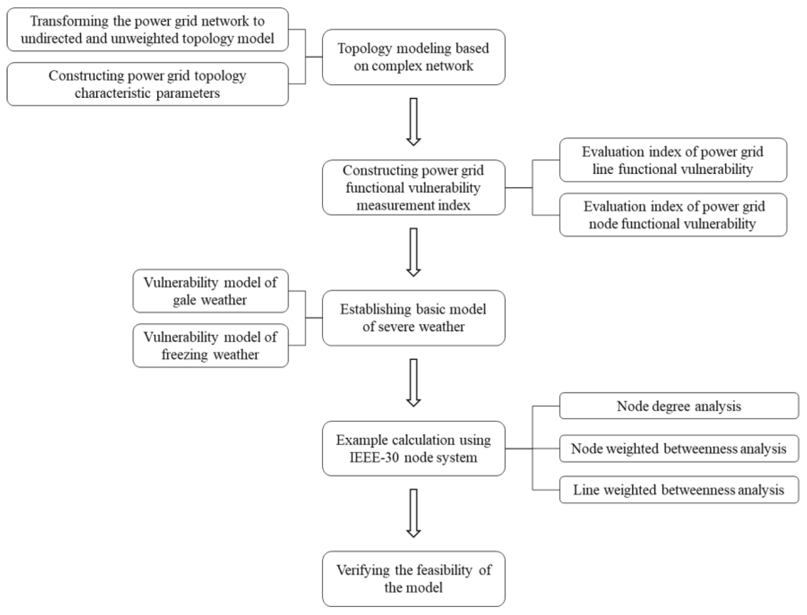
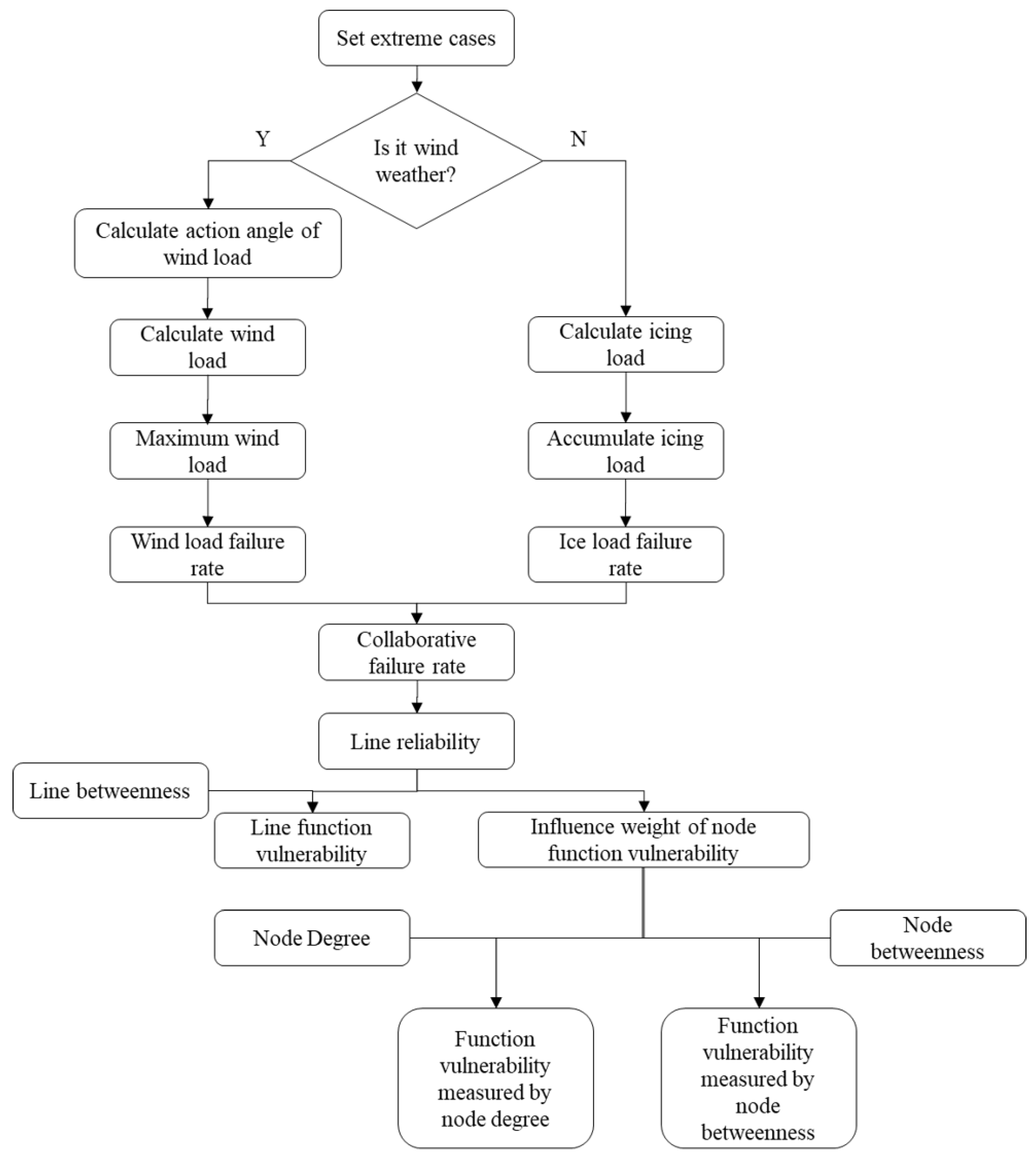
The results of the final example analysis indicate that our proposed model can serve as theoretical support for the research field of power grid large-scale faults under extreme conditions, improving the adaptability of traditional models to different situations so as to fit the real situation. The framework of the proposed method is shown in Figure 1.

The rest of this paper is constructed as follows. Section 2 presents the research status related to extreme weather and power grid functional vulnerability. Section 3 and Section 4 introduce the power grid topology modeling method based on complex network modeling and power grid functional vulnerability based on reliability, respectively. Section 5 performs an example analysis using the IEEE-30 node system. The final analysis and conclusion are presented in Section 6.

2. Related Work

There is extensive relevant research on the functional vulnerability of power grid units and relevant theoretical models under extreme weather. Extreme weather is the main influence on power grid failure. The general modeling methods of power grid reliability, vulnerability, and resilience under extreme weather are two-state models and three-state models according to the severity of extreme weather, performing a comparative analysis of reliability under different weather conditions [20].

The influences of extreme weather on the reliability and vulnerability of the power grid are mainly the destruction and increased failure rate of power grid units. Zhou T. et al. [21] utilized the detrended fluctuation method to analyze the impact of extreme weather conditions on grid unit failures. Billiton R. et al. [22] researched the normal case and the extreme weather of a gale disaster simultaneously, obtaining the grid reliability models under the two states through comparative analysis. R. Billinton et al. [23] established a three-state climate model to study the reliability of the power grid. Lightning weather [24,25], gale weather [26,27], and line icing [28,29,30] were separately researched to search the impact on power grid reliability. Yong Liu et al. [31] integrated the extreme conditions of gale disasters and lightning, studying the reliability models under different severities. Bhuiyan M. R. et al. [32] integrated the three-state climate model into the establishment of the failure rate model, in which the weather superposition state of transmission lines was considered at the same time, and the Monte Carlo method was utilized to sample and simulate the climate region and unit state. Kiel E. S. et al. [33] connected severe weather with power grid vulnerability, exploring the influence of severe weather on the power system reliability index through the failure rate model.

Power grid resilience involves the four stages of anticipation, absorption, recovery, and adaptability, and each stage is easily influenced by extreme weather. The energy management system, optimal power flow, and dynamic control are widely applied to the resilience modeling of the power grid under extreme weather [34]. In terms of frequently concerning typhoon weather, Nguyen H. T. et al. [35] utilized a stochastic optimization model based on resilience improvement, and Zhou J. et al. [36] proposed a coordinated optimization method based on the regional integrated energy system to realize resilience improvement. The mathematical programming model is an important optimization method to study the resilience of power grid; Hou H. et al. [37] used machine learning methods to analyze the impact of wind disasters on transmission lines, and Karangelos E. et al. [38] combined the failure rate of grid units sensitive to weather with an optimization model based on vulnerability identification through the Monte Carlo method. Under extreme weather, the power grid capabilities related to resilience include physical hardiness and operational capability, and each capability enhancement strategy improves the overall power grid system resilience [39]. With the rapid development of smart grid technology, the power grid resilience evaluation method based on modularity can effectively reduce the failure rate of power grid units under extreme weather [40].

In the above works researching the impact of extreme weather on the power grid, the extreme weather considered is limited, mainly focusing on lightning, icing, and gale disasters, and it lacks consideration of extreme conditions with the synergism of multi-disaster competition. In particular, most case studies of power grid resilience have been carried out under stormy weather. In the research on power grid reliability and vulnerability, although the failure rate of power grid units in different extreme weather conditions is taken into account, there are few specific physical models carried out in quantitative research.

Various research methods describing the different characteristics of power grid units have attracted more and more attention in terms of power grid functional vulnerability. Functional vulnerability analysis methods can be divided into complex network theory and power flow analysis. Nima Amja et al. [41] studied node voltage vulnerability based on energy function. Ubeda J. R. et al. [42] studied power grid functional vulnerability using an analytical method, yet this method failed to work when there were many network nodes with high complexity; this can be solved through the Monte Carlo method when the complexity of the power grid is high. Singh C. et al. [43] modeled reliability based on the uncertainty probability and guarantee time of hidden failure. Yu Xingbin et al. [44] defined grid vulnerability parameters, including the bus isolation rate, load loss rate, and load reduction expectation, and proposed a functional vulnerability evaluation index of the system level based on these parameters. By analyzing the cascading failure model of the power grid based on the Monte Carlo method, Su Sheng et al. [45] identified the key vulnerable nodes of the power grid system and optimized the distribution of system compensation devices. However, although the Monte Carlo method can deal with the high complexity of the power grid, it also brings a huge computational burden. Nan L. et al. [46] proposed a vulnerability analysis method considering both topological and functional characteristics of the power grid to identify vulnerable units. Liu Y. et al. [47] evaluated the dependence between grid units using a dynamic network flow redistribution model. Functional vulnerability deeply studies the dynamic process of cascading faults; Abedi A. et al. [48] established a power flow model by introducing a novel vulnerability assessment index to analyze cascading faults, and Fang J. et al. [49] designed a multi-objective optimization algorithm to evaluate power grid vulnerability with regard to cascading faults. Among the methods above, the functional vulnerability of the power grid is rarely analyzed from the physical and mechanical points of view.

The existing research rarely combines the power grid functional vulnerability with extreme weather, which makes the modeling deviate from reality and unable to effectively study the power grid cascading fault mechanism.

Table 2. The deficiencies of existing research on extreme weather acting on the power grid and functional vulnerability.

Research Contents	Major Method	Deficiencies of Existing Researches
Extreme weather	Multi-state climate model	The weather scenario of the case analysis is too singular, and there are few quantitative studies through physical modeling
Power grid functional vulnerability	Complex network theory and power flow analysis	A physical and mechanical model is rarely established to analyze the power unit’s specific characteristics

presents some details in the investigated literature on extreme weather and functional vulnerability. Identifying how to carry out topology modeling that fits the reality is the major challenge when analyzing vulnerability; this means it must fully consider related physical and mechanical characteristics. Therefore, extreme conditions with the synergism of multi-disaster competition need to be considered to analyze power grid functional vulnerability. Complex network modeling is an efficient modeling method for the power grid that does not ignore significant characteristic information of the power grid during simulation [50]. In conclusion, in this paper, we used the complex network topology theory to model the power grid according to the deficiencies of existing research. The extreme weather of gale and freezing was considered, and the feasibility of the proposed topology model was verified by the quantitative analysis of an example.

3. Power Grid Topology Modeling Based on Complex Network Modeling

3.1. Topology Modeling Rules

In order to study the vulnerability of the power grid from a macro perspective, the first task is to transform the power grid structure into a topology model based on graph theory.

According to the structure and characteristics of different types of power grid units, power grid units are divided into two types represented by nodes and edges following the common modeling method, forming a powerless undirected topology model. First, the generator, transformer, and user load are taken as network nodes with a total number n while modeling, which are divided into three categories according to the energy flow direction, including the source node set S_G, the sink node set S_L, and the link node set S_t. Then, the high voltage line L_G and the transformer branch L_T are regarded as the edges with a total number k. The nodes connecting each edge are denoted by i and j, and the n-order incidence matrix A is defined to represent the connection relationship between nodes. The element of the i-th row and j-th column in matrix A is the connection coefficient a_ij.

$$A=\left(\begin{array}{cccc}{a}_{11}& a_{12}& \cdots & a_{1n}\\ a_{21}& a_{22}& \cdots & a_{2n}\\ ⋮& ⋮& \ddots & ⋮\\ a_{n1}& a_{n2}& \cdots & a_{nn}\end{array}\right)$$

(1)

When $i=j$ or there is no connecting edge i and j, the value of a_ij is 0. Otherwise, the value of a_ij is 1.

From a macro perspective, on the premise of ensuring that it is suitable for the actual case, the model is appropriately simplified through the following three steps: (1) the power grid structure is simplified, mainly considering the 220 kV and above high-voltage transmission network; (2) the parallel lines on the same tower are merged, and the shunt capacitor lines are ignored to eliminate the case of multiple edges and self-direction in the power grid; and (3) regardless of the internal physical properties of each unit, all grounding wires are ignored.

In the undirected and unweighted topology model, the attributes of all nodes are the same, the energy can be transmitted along the edges of the network in two directions, and the weight of each edge is set to 1 [51,52]. When there is a parallel connection, the same number of edges leads to the same weight for multi-path, which makes it difficult to determine the minimum path and has a great impact on the analysis of network parameters.

In order to better adapt to reality, the power grid node is divided into three types: when the output power of the node is greater than the load power, the node is the source node; when the output power of the node is smaller than the load power, the node is the sink node; and other nodes are link nodes. Energy can only be transferred from the node with higher potential to the node with lower potential, transforming the undirected topology model into the directed topology model. The reactance value x_ij0 is equivalent to the edge weight w_ij, the effect of reactance is similar to that of the resistance in a direct current. When the reactance value of the line is larger, the transmitted power is smaller, transforming the unweighted topology model is into a weighted topology model. The n-order weighted square matrix W is redefined to represent the connection relationship between nodes while weighting. The element of i-th row and j-th column in the matrix W is W_ij:

$$W=\left(\begin{array}{cccc}{w}_{11}& w_{12}& \cdots & w_{1n}\\ w_{21}& w_{22}& \cdots & w_{2n}\\ ⋮& ⋮& \ddots & ⋮\\ w_{n1}& w_{n2}& \cdots & w_{nn}\end{array}\right)$$

(2)

When i is equal to j, the value of W_ij is 0, and when $i\ne j$ and there is a direct connecting edge between i and j, the value of W_ij is equal to x_ij. Otherwise, the value of W_ij is infinite.

3.2. Characteristic Parameters of Power Grid Topology Model

After network weighting, the distance d_ij between node i and node j is the reactance sum of the edges contained in the shortest path between two nodes. The weights of edge ij and edge jk are w_ij and w_jk, respectively, and Equation (3) can be deduced to calculate the distance d_ik between nodes i and k. The network average distance L is obtained from the average distance of all pairs of nodes.

$$d_{ik}=w_{ij}+w_{jk}$$

(3)

$$L=\frac{1}{\frac{1}{2}n(n-1)}{\displaystyle \sum _{i\ne j}{d}_{ij}}$$

(4)

The weighted betweenness, measuring the importance of nodes and edges in the whole network, is divided into node betweenness C_Bv and edge betweenness C_Be. Node betweenness C_Bv is the proportion of the weighted shortest paths passing through a node in the network to all the weighted shortest paths in the network. Edge betweenness C_Be is the proportion of the weighted shortest paths passing through an edge in the network to all the weighted shortest paths in the network.

$$C_B{}_v=\frac{{\displaystyle \sum _{i\ne v\ne j}{\sigma }_{ij}{}_v}}{{\displaystyle \sum _{i\ne j}{\sigma }_{ij}}}$$

(5)

$$C_B{}_e=\frac{{\displaystyle \sum _{i\ne j}{\sigma }_{ij}{}_e}}{{\displaystyle \sum _{i\ne j}{\sigma }_{ij}}}$$

(6)

where ${\sigma }_{ij}$ refers to the number of shortest paths between node i and node j, and ${\sigma }_{ij}{}_v$ and ${\sigma }_{ij}{}_e$ are the number of shortest paths between node i and node j containing node v or edge e, respectively.

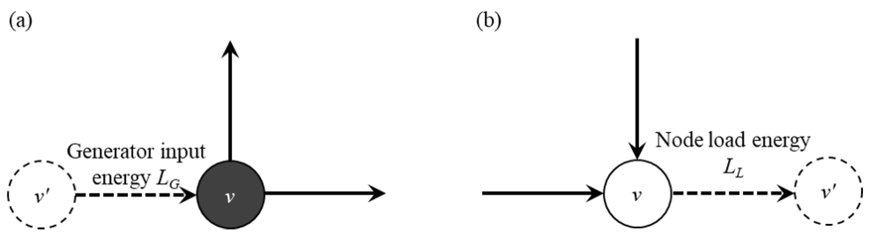
When node v is the link node, the number of shortest paths to enter node v is equal to the number of shortest paths to leave node v, which can be directly calculated by Equation (6). If node v belongs to the source node, the path only leaves from this node, as the source node is the starting node of the shortest path, leaving the number of shortest paths entering the node less than that leaving the node. In the same way, if node v belongs to the sink node, the number of shortest paths entering the node is larger than that leaving the node. In this case, a virtual node is introduced to transform node v into a link node, as shown in Figure 2.

When the node v is the source node, the shortest path from v to any sink node only leaves from the edge and does not enter from the edge. The betweenness C_BG of source node v is as follows:

$$C_B{}_G=C_{Bv}+\frac{1}{2}{n}_L$$

(7)

where n_L is the number of sink nodes.

When node v is the sink node, the shortest path from any source node to v only enters from the edge and does not leave from the edge. The betweenness C_BL of sink node v is as follows:

$$C_B{}_L=C_{Bv}+\frac{1}{2}{n}_G$$

(8)

where n_G is the number of source nodes.

In the reactance weighted network, the node degree k_i, which is defined as the number of edges connected to the node, remains unchanged. The average degree K of a network is the average degree of all nodes and edges k_i.

$$K=\frac{1}{n}{\displaystyle \sum k_i}$$

(9)

3.3. Power Grid Topology Modeling and Characteristic Parameter Analysis Process

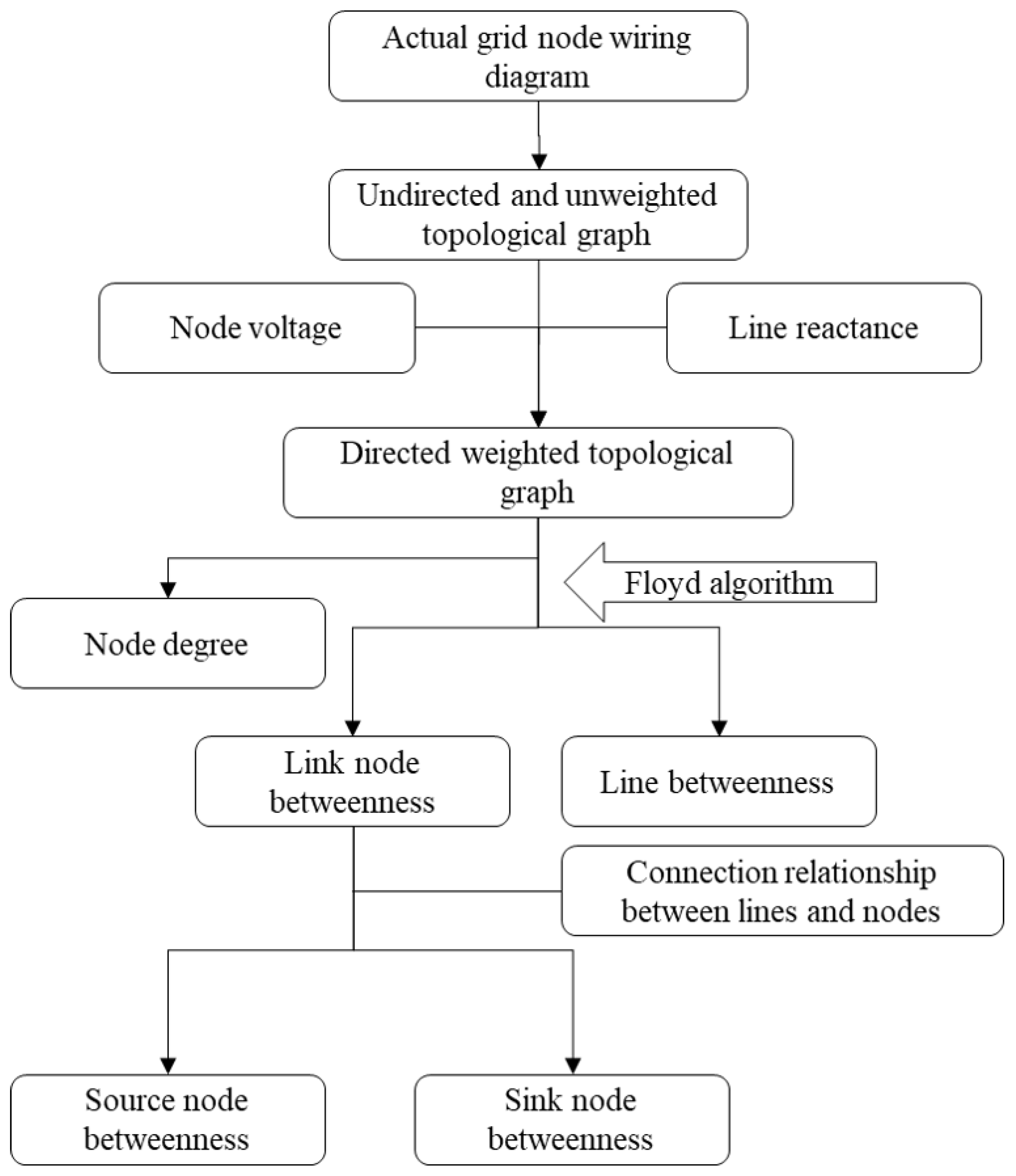
The process of power grid topology modeling and characteristic parameter analysis is shown in Figure 3, and the detailed steps are as follows:

Step 1: The actual power grid model is transformed into the power grid topology model according to power grid topology modeling rules in Section 3.1. The abstract class element is established, and then the node subclass and link subclass are established to store the initial data of the node and line, based on which the weighted model is established.

Table 3. Class attribute information.

Abstract Class Element
Attribute	Description	Attribute	Description
id	Number	state	State
betweenness	Weighted betweenness	capacity	Capacity
fragile_b	Vulnerability measured by betweenness	load	Load
Class Node		Class Link
Attribute	Description	Attribute	Description
weight	Weight influencing Vulnerability	reliability	Reliability
degree	Degree	pre_node	Previous node
point_x	Node abscissa	suc_node	Succeeding node
point_y	Node ordinate	reactancex	Reactance value
power_out	Generator output power	length	Line length
power_in	Node load power	——	——
fragile_d	Vulnerability measured by degree	——	——

shows the data structure information of the nodes and lines in the power grid topology model.

Step 2: All nodes are traversed, and then the value of power_out and power_in are judged. Nodes are divided into the source node, sink node, and link node, and then the directed weighted model is obtained.

Step 3: The characteristic parameters of the power grid are analyzed. The nodes and the line in the loop are traversed. When the traversed node is the previous node, the leaving degree increases by one. Similarly, if the traversed node is the succeeding node, the entering degree increases by one. The node degree is the sum of the entering degree and the leaving degree.

Step 4: The Floyd algorithm is applied to calculate the minimum distance between nodes. In the line reactance matrix, the nodes are traversed from the top left to the bottom right. If there is a direct connection between the node pairs, the distance between the node pairs is the line reactance. Conversely, if there is no direct connection, the distance between the node pairs is determined by Equation (3), and the shortest distance between the node pairs is obtained by traversing all nodes.

Step 5: The number of link nodes appearing in the node pair is counted while traversing the nodes. If the node is a source node, the betweenness is half the value calculated by the number of link nodes plus the number of sink nodes, according to Equation (7). If the node is a sink node, the betweenness is the half the value calculated by the number of link nodes plus the number of source nodes, according to Equation (8).

Step 6: The characteristic parameters of the nodes and lines are ranked, the cumulative distribution diagram is drawn.

In this paper, the power grid nodes were divided into the source node, sink node, and link node according to the relationship between the energy inflow and outflow, and the line reactance value was introduced to transform the model into a directed weighted model. The characteristic parameters of power grid units were analyzed by the calculation method of reset betweenness, laying the foundation for the calculation of power grid vulnerability.

4. Power Grid Functional Vulnerability Based on Reliability

4.1. Evaluation Index of Power Grid Functional Vulnerability

4.1.1. Evaluation Index of Power Grid Lines Functional Vulnerability

The function vulnerability of the power grid system is defined as the disturbance degree to the function of the power grid unit in the specified time conditions. It is crucial to select the appropriate topology weight of power grid units when measuring functional vulnerability. When an extreme condition occurs, the external environment conditions and the state of the power grid unit vary, and the frequency of this variation is faster compared with the normal case. When the original betweenness index is used to measure the functional vulnerability of the power grid, it is difficult to measure the disturbance of the external environment to the power grid units under extreme conditions. However, the node vulnerability obtained from the betweenness analysis in the normal case may not be consistent with the actual load level or the reliability under extreme conditions. In particular, the node vulnerability in the normal case is low, yet the actual load is very large and the reliability under extreme conditions is low, leading to high risk. Therefore, the power grid functional vulnerability model based on reliability was established according to reference [46], and the time parameters were selected to weigh the power grid functional vulnerability. Under extreme conditions, if there is no time to repair the power grid lines in a short period of time, the unit reliability R_i can be calculated following Equation (10):

$$R_i(t)=\exp (-{\displaystyle {\int }_0^t{\lambda }_{i0}(x)dx)}$$

(10)

where the reliability R_i is a function of time t, λ_i0 is the unit failure rate (1/h).

When the reliability of the element obeys exponential distribution, the unit failure rate λ_i0 is a constant. The reliability R_i can be obtained from Equation (11).

$$R_{\mathrm{i}}(t)=\exp (-{\lambda }_{i0}t)$$

(11)

According to the above modeling, in the weighted network, the line functional vulnerability B_Bei is defined as the product of unit unreliability F_ei and betweenness B_ei:

$$B_{Be}{}_i=F_{ei}\times B_e{}_i=(1-R_e{}_i)\times B_e{}_i$$

(12)

where the unreliability F_ei can be obtained from the reliability R_ei. The unreliability F_ei is selected to measure the power grid functional vulnerability, for which the unreliability F_ei is directly proportional to the vulnerability. The larger F_ei is, the more vulnerable the unit becomes. The reliability R_ei is inversely proportional to the vulnerability.

4.1.2. Evaluation Index of Power Grid Node Functional Vulnerability

Under extreme conditions, power grid nodes will be affected by line load fluctuations in the operation of the power grid system, on which the influence of the neighborhood cannot be reflected through the original betweenness index measuring functional vulnerability [53]. Therefore, the functional vulnerability measured by the node degree B_Dvi is defined as the product of the power grid line influence weight on the node F_vi and the node degree k_i.

$$B_{Dv}{}_i=F_{vi}\times k_i$$

(13)

The functional vulnerability under extreme conditions measured by the betweenness of power grid nodes is defined as the product of power grid line influence weight on the node F_vi and the node betweenness B_vi.

$$B_{Bv}{}_i=F_{vi}\times B_v{}_i$$

(14)

The influence weight of the power grid line on the nodes F_vi is defined as follows. The lines flowing through the nodes are divided into the current inflow line set E_in and the current outflow line set E_out according to the sign of the current. In this paper, the reliability of the inflow line set E_in and the outflow line set E_out were calculated in order. Using E_in as an example, E_in is composed of M elements (e_in1, e_in2, ..., e_inm). The influence weight of the grid node inflow F_in is defined as Equation (15).

$$F_{in}=1-\frac{1}{m}{{\displaystyle \sum }}^{ }{R}_{ei}\left(t\right)$$

(15)

where R_ei(t) is the reliability of unit e_i, and the calculation method of F_out is as same as F_in.

Only when the two subsystems of inflow, line set E_in and outflow line set E_out, are both normal is the system in the normal state. Therefore, the system conforms to the series system model, and the influence weight F_vi of power grid nodes is defined as Equation (16).

$$F_{vi}=1-\left(1-F_{in}\right)\left(1-F_{out}\right)$$

(16)

If the node v is the source node or the sink node, either F_in or F_out does not exist, and the influence weight of the source node F_Gi is defined as Equation (17).

$$F_{Gi}=1-{(1-F_{out})}^2$$

(17)

Similarly, the grid node influence weight of sink node F_Li is defined as Equation (18).

$$F_{Li}=1-{(1-F_{in})}^2$$

(18)

4.2. Power Grid Functional Vulnerability under Extreme Weather

4.2.1. Basic Model of Severe Weather

As a country with vast territory, a complex climate, and a large temperature difference between the South and the North, there are extensive differences in climate and natural disasters in China. In addition, there are many trans-regional and long-distance transmission facilities in the power grid system, most of which are constructed in open air and greatly affected by the climate, causing the occurrence of extreme weather disturbances to be more frequent and the grid functional vulnerability to be far higher than the normal case [54]. According to the standard of the IEEE 346, weather intensity is divided into the following three types: normal weather, severe weather, and extreme severe weather [55]. When the grid unit is exposed to different weather intensities, the corresponding failure rate is different. The types of severe weather mainly include freezing, gale, lightning, rainstorm, and drought, of which freezing and gale are the major causes of power grid unit failure [56,57].

The occurrence of severe weather has obvious regional and temporal characteristics. In China, gale disasters mainly occur in the coastal areas of the South and East, and freezing disasters mainly occur in the northeast, north, and central regions. Therefore, the ability of transmission lines to withstand severe weather in different regions is different because of the different geographical locations and meteorological conditions. The geographical and seasonal factors endow a certain time characteristic to severe weather, resulting in the concentrated occurrence of specific severe weather conditions. Ice disasters often occur in winter, and gale weather occurs in summer and winter. By contrast, the frequency of severe weather in the spring and autumn is lower, and the intensity is lower than that in the summer and winter.

In summary, the impact of extreme conditions caused by gale weather and freezing weather on the functional vulnerability of the power grid is the major research direction of this paper. According to the relationship among line operation conditions, the line load, and its own attributes, the calculation model of line functional vulnerability was established. A node functional vulnerability calculation model was established to analyze the vulnerability distribution of the power grid system under extreme weather based on the relationship between the current inflow and outflow lines, together with the reliability of the power grid nodes.

The ice storm weather load model was analyzed consistent with [58], utilizing the circle model with maximum central strength to express the load of a transmission line section. The bivariate function in the following formula has appropriate properties and can be regarded as the basic model to describe the wind load and freezing load:

$$f(x_j,y_j)=A\exp (-\frac{1}{2}({(\frac{x_j-{\mu }_x}{{\sigma }_x})}^2+{(\frac{y_j-{\mu }_y}{{\sigma }_y})}^2))$$

(19)

where A refers to weather severity (amplitude), μ_x and μ_y are the coordinates of weather center, and σ_x, σ_y are the load calculation parameters related to the influence radius of weather.

4.2.2. Vulnerability Model of Gale Weather

The main influencing factor in gale weather is the wind load in the power grid. The wind load refers to the instantaneous wind force in severe weather, also known as gust wind. Since the wind load is 0 at the absolute center of the storm, Equation (19) is not applicable. A more practical model is obtained by subtracting an extra function with a smaller amplitude A and load calculation parameter σ [59].

$$\begin{array}{cc}\hfill L_W(x_j,y_j,t)& =w(t)(A_1\exp (-\frac{1}{2}({(\frac{x_j-{\mu }_x(t)}{{\sigma }_{x1}})}^2+{(\frac{y_j-{\mu }_y(t)}{{\sigma }_{y1}})}^2))\hfill \\ & -A_2\exp (-\frac{1}{2}({(\frac{x_j-{\mu }_x(t)}{{\sigma }_{x2}})}^2+{(\frac{y_j-{\mu }_y(t)}{{\sigma }_{y2}})}^2)))\hfill \end{array}$$

(20)

where w is the influence of wind direction on transmission line wind load, A₁ and A₂ are parameters of gale weather severity (A₁ > A₂), and σ_x1, σ_y1, σ_x2, σ_y2 are load calculation parameters (σ_x1 > σ_x2, σ_y1 > σ_y2).

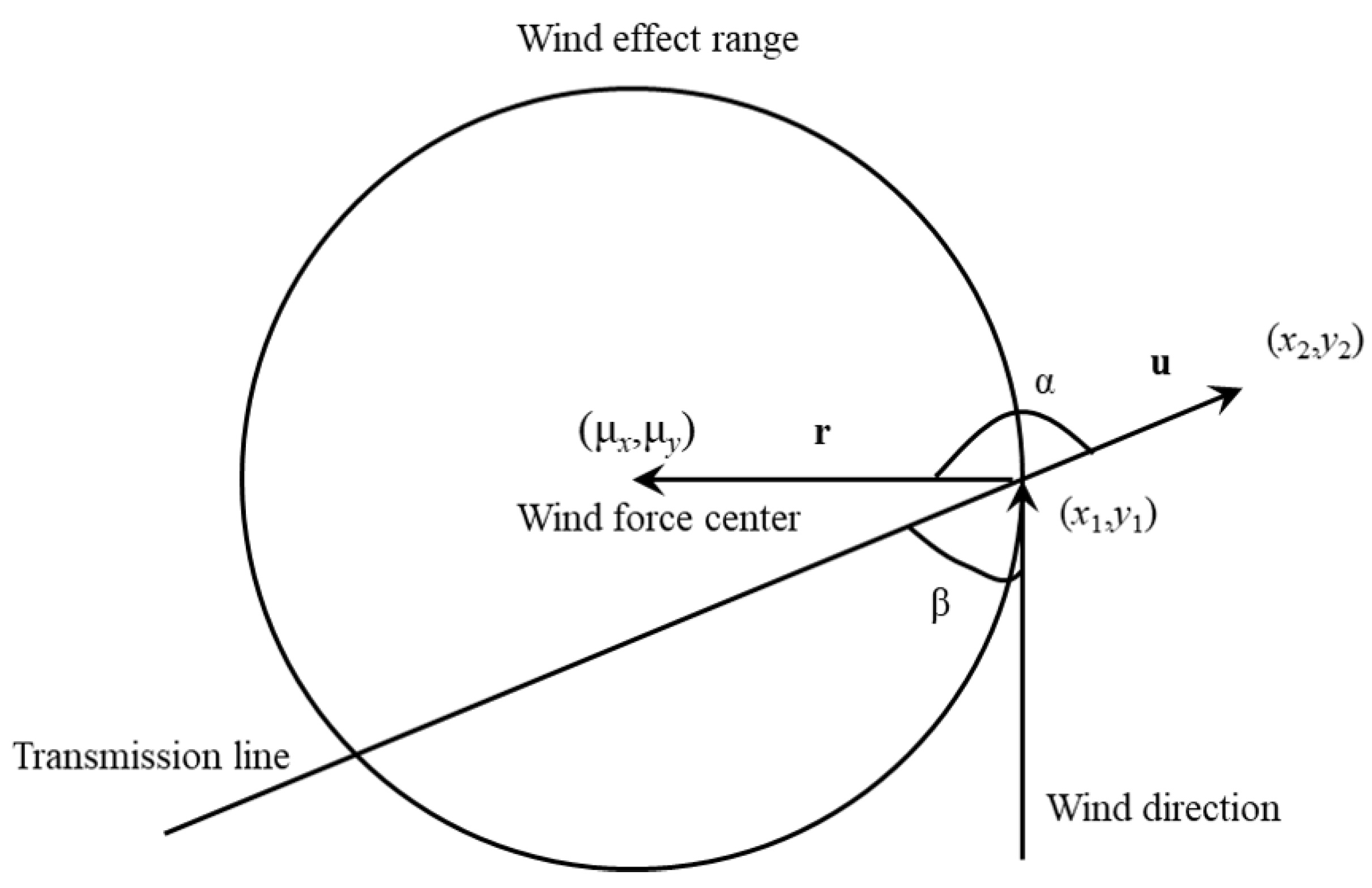
In Equation (20), the influence of wind direction on transmission line wind load w(t) considers the wind direction factor composed of the angle β between the wind direction and the transmission line. In the northern hemisphere, the wind direction rotates anticlockwise around the weather center, perpendicular to the wind load of the power grid line. Therefore, the worst weather case is represented by β = π/2. Figure 4 shows the relative position between the line and the weather center as well as the effect of the wind load.

In Figure 4, α is the angle between vector $r=[(x_1,y_1),({\mu }_x,{\mu }_y)]$ and vector $u=[(x_1,y_1),(x_2,y_2)]$. The wind direction is always perpendicular to vector r, and the angle β between the wind direction and the transmission line is acute or right.

$$\alpha =\arccos \frac{ru}{\left|r\right|\left|u\right|}$$

(21)

$$\beta (t)=\{\begin{array}{l}\frac{\pi }{2}-\alpha , \alpha \le \frac{\pi }{2}\\ \alpha -\frac{\pi }{2}, \alpha >\frac{\pi }{2}\end{array}$$

(22)

The influence of the wind direction on the wind load of the transmission line is as follows:

$$w(t)=\sin \beta (t)$$

(23)

When β is 0, the wind load influence coefficient is 0, for which the wind load parallel to the line will not affect the line in practice. When the line is vertically subjected to the wind load, β is $\pi /2$. The influence coefficient of the wind load is 1, indicating that the wind load has the greatest influence at this time.

The line failure rate under extreme weather λ_W (times/h, KM) is related to the line wind load.

$${\lambda }_W(t)=f(L_W(t))$$

(24)

According to reference [60], the discrete relationship between the wind load and the line failure rate under extreme weather is calculated as shown in

Table 4. Corresponding relationship between the line failure rate and the wind load.

LW	λW (Times/h, 50 KM)
LW ≤ 0.9 dlW	1.2 × 10−5
0.9 dlW < LW ≤ 1.0 dlW	8.0 × 10−4
1.0 dlW < LW ≤ 1.1 dlW	0.048
1.1 dlW < LW ≤ 1.2 dlW	0.060
1.2 dlW < LW ≤ 1.5 dlW	0.028
1.5 dlW < LW	0.04

, in which dl_W is the line design value of the wind load.

4.2.3. Vulnerability Model of Freezing Weather

The main influencing factor in freezing weather is the icing of power grid lines. Icing will lead to an increase in the line load, leading to a change in the conductor cross-section and even the collapse of the high-voltage line tower, broken lines, and relaxation of the vibration of the iced line [60,61]. According to Equation (19), the ice load of power grid lines should also be related to the degree of severe weather and the distance from the line to the weather center. However, the ice load caused by icing is a cumulative process and is related to the duration of freezing weather. As shown in Equation (25), it can be feasible to solve the above problems using integrals.

$$L_I(x_i,y_i,t)={\displaystyle {\int }_0^t{A}_3\exp (-\frac{1}{2}({(\frac{x_i-{\mu }_x(u)}{{\sigma }_x})}^2}+({(\frac{y_i-{\mu }_y(u)}{{\sigma }_y})}^2))du$$

(25)

where A₃ is a parameter of the freezing weather severity.

If only considering the influence of ice load and ignoring the melting of ice in a short time under extreme weather, the ice load of the line increases with the duration of extreme weather until the freezing weather does not affect the line and the ice load reaches the maximum, becoming constant.

The line failure rate under extreme weather λ_I (times/h, KM) is related to the line ice load.

$${\lambda }_I(t)=f(L_I(t))$$

(26)

The discrete relationship between the ice load and the line failure rate under extreme weather can be obtained according to

Table 5. Corresponding relationship between the line failure rate and the ice load.

LI	λI (Times/h, 50 km)
LI ≤ 0.3 dlI	0
0.3 dlI < LI ≤ 0.5 dlI	4.5 × 10−3
0.5 dlI < LI ≤ 0.9 dlI	0.010
0.9 dlI < LI ≤ 1.0 dlI	0.015
1.0 dlI < LI ≤ 1.1 dlI	0.033
1.1 dlI < LI ≤ 1.2 dlI	0.050
1.2 dlI < LI ≤ 1.5 dlI	0.071
1.5 dlI < LI	0.10

[61], in which dl_I is the line design value of the ice load.

4.2.4. Collaborative Vulnerability Model of Gale and Freezing Weather

Gale and freezing weather often occur together in winter, leaving power grid lines to bear both a wind load and an ice load. Moreover, the failure modes of the wind load and the ice load act on the power grid lines independently. Therefore, this collaborative vulnerability model conforms to the competitive fault model:

$$\lambda =a_W{\lambda }_W+a_I{\lambda }_I$$

(27)

where λ is the total failure rate, and a_W, a_I are the influence weights of wind load and ice load, respectively.

4.3. Power Grid Functional Vulnerability Analysis Process

The process of the power grid functional vulnerability analysis is shown in Figure 5, and the detailed steps are as follows:

Step 1: Set the type of extreme situation. In this paper, the extreme case was freezing and gale weather, and the calculations of freezing weather and gale weather were carried out respectively. Set the extreme case parameters, initial position, and wind direction.

Step 2: Traverse the line and calculate the load of the line under the wind force. Set the duration of wind force, calculate the angle between the line and wind direction according to Equations (21)–(23), and then calculate the load according to Equation (20). Finally, record the maximum load of each line within the duration.

Step 3: Traverse the line and calculate the load of the line under the action of freezing. Set the freezing action time, accumulate the line load under freezing action according to Equation (25), and finally, record the maximum load of each line within the duration.

Step 4: Calculate the line failure rate according to Equation (27).

Step 5: Calculate the line reliability and the functional vulnerability measured by betweenness according to Equations (10)–(12).

Step 6: Traverse the nodes and calculate the node function vulnerability influence weight according to Equations (15)–(19). Then, calculate the degree and betweenness to measure the node functional vulnerability according to Equations (13) and (14).

Step 7: Traverse the nodes and edges, ranking the functional fragility.

The calculation method of unit functional vulnerability under extreme weather was constructed in this paper. Focusing on the typical extreme weather of gale weather and freezing weather, the load of the line section in these two cases was constructed, which was converted into the failure rate according to a certain functional relationship. Then, the line reliability was obtained and multiplied by the weighted betweenness of the line to obtain the line functional vulnerability. The node influence weight was obtained using the line reliability and multiplied by the node degree and betweenness to obtain the node reliabilities measured by degree and betweenness, respectively.

5. Example Analysis

In this paper, the IEEE-30 bus system was applied to the example analysis. First, the topology of the power grid was modeled to obtain the characteristic parameters. Then, the functional vulnerability and structural vulnerability of the power grid were calculated to analyze the vulnerability of the power grid load imbalance under extreme weather. Last, the constructed model was verified through a simulation experiment.

5.1. Power Grid Topology Modeling and Characteristic Parameter Analysis

5.1.1. Power Grid Topology Modeling

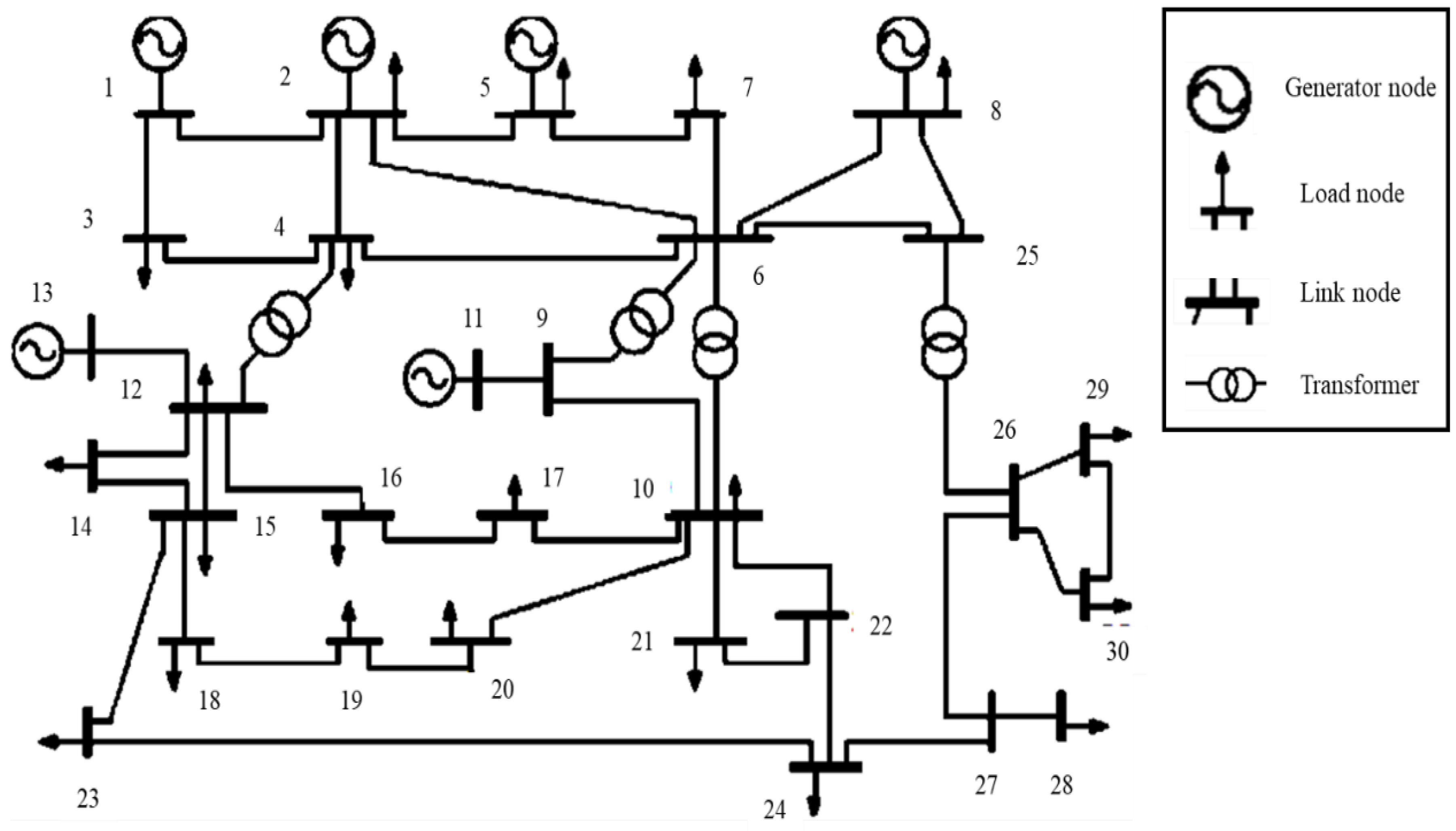
Figure 6 shows the wiring diagram of the IEEE-30 system, which is composed of 30 nodes and 41 lines. The nodes can be divided into 5 source nodes, 19 sink nodes, and 6 link nodes, according to their properties. Specifically, although node 5 is both an engine node and a load node, its load power is greater than its generator input power, which means that node 5 is a sink node. The specific type of each node is shown in

Table 6. IEEE-30 system node types.

Node Type	Node Number	Node ID
Source node	5	1, 2, 8, 11, 13
Sink node	19	3, 4, 5, 7, 10, 12, 14, 15, 16, 17, 18, 19, 20, 21, 23, 24, 28, 29, 30
Link node	6	6, 9, 22, 25, 26, 27

.

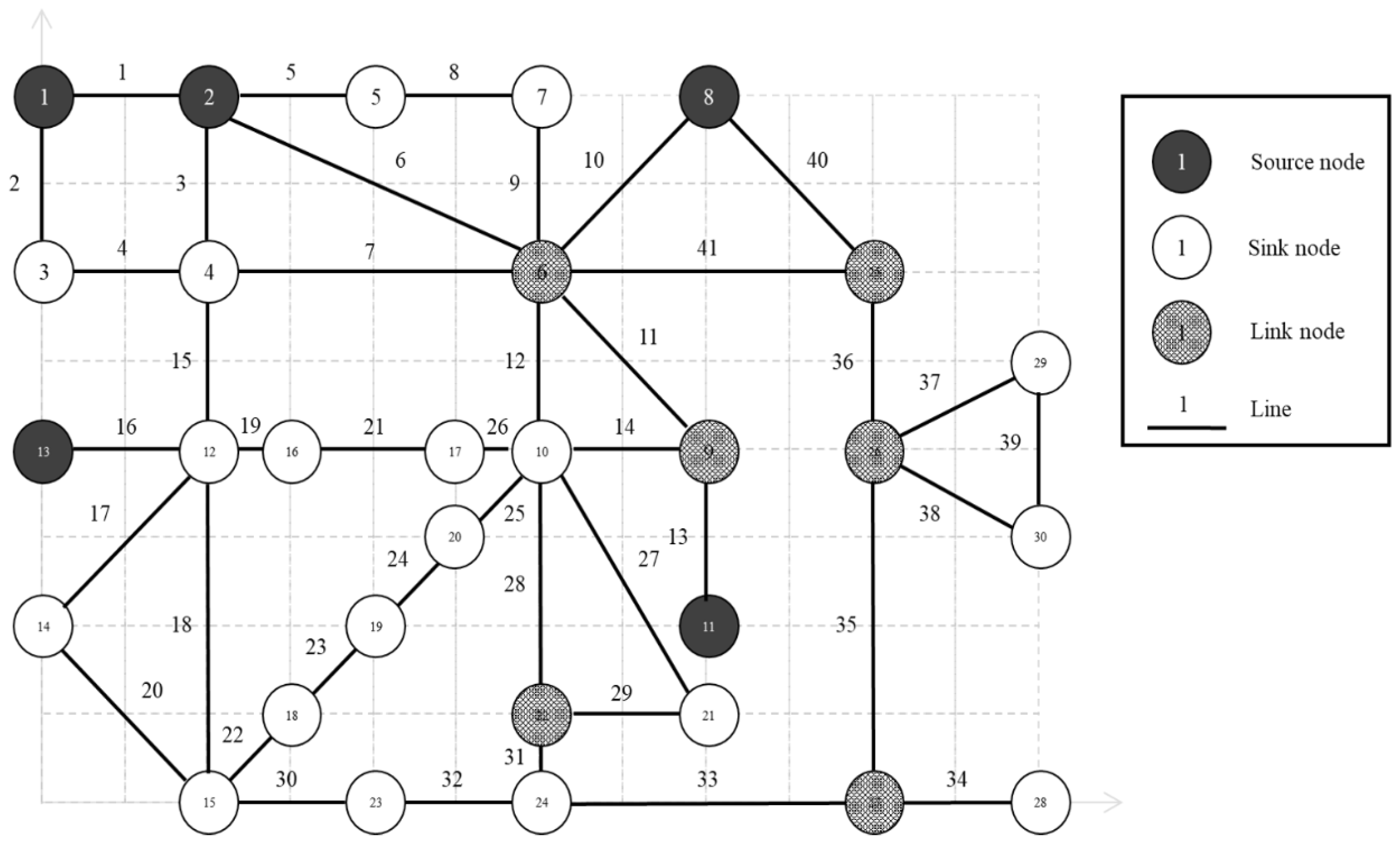
The topology model of the power grid was established according to Section 3, transforming the power grid into a directed weighted topology model. Figure 7 shows the schematic diagram of the IEEE-30 system topology model, in which the coordinate axis is established, and the unit length is 50 km. The nodes and lines are labeled, and the coordinate positions were determined respectively, distinguished by different colors according to node types.

5.1.2. Characteristic Parameter Analysis

All the lines of the power grid were traversed in turn, accumulating the occurrence times of each node in the previous node and subsequent nodes of the line.

If the occurrence time in the previous nodes of node v is m, the leaving degree of node v is m. Similarly, if the occurrence time in the subsequent nodes of node v is n, the entering degree of node v is n. The node degree is the sum of the entering degree and leaving degree.

Table 7. Node degree ranking.

Ranking	Node ID	Node Degree
1	6	7
2	10	6
3	12	5
4	4	4
4	2	4
4	15	4
4	27	4

indicates the ranking of the top seven nodes by degrees, and it is obvious that the nodes with larger degrees connect more lines, approach more neighboring nodes, and bear heavier loads.

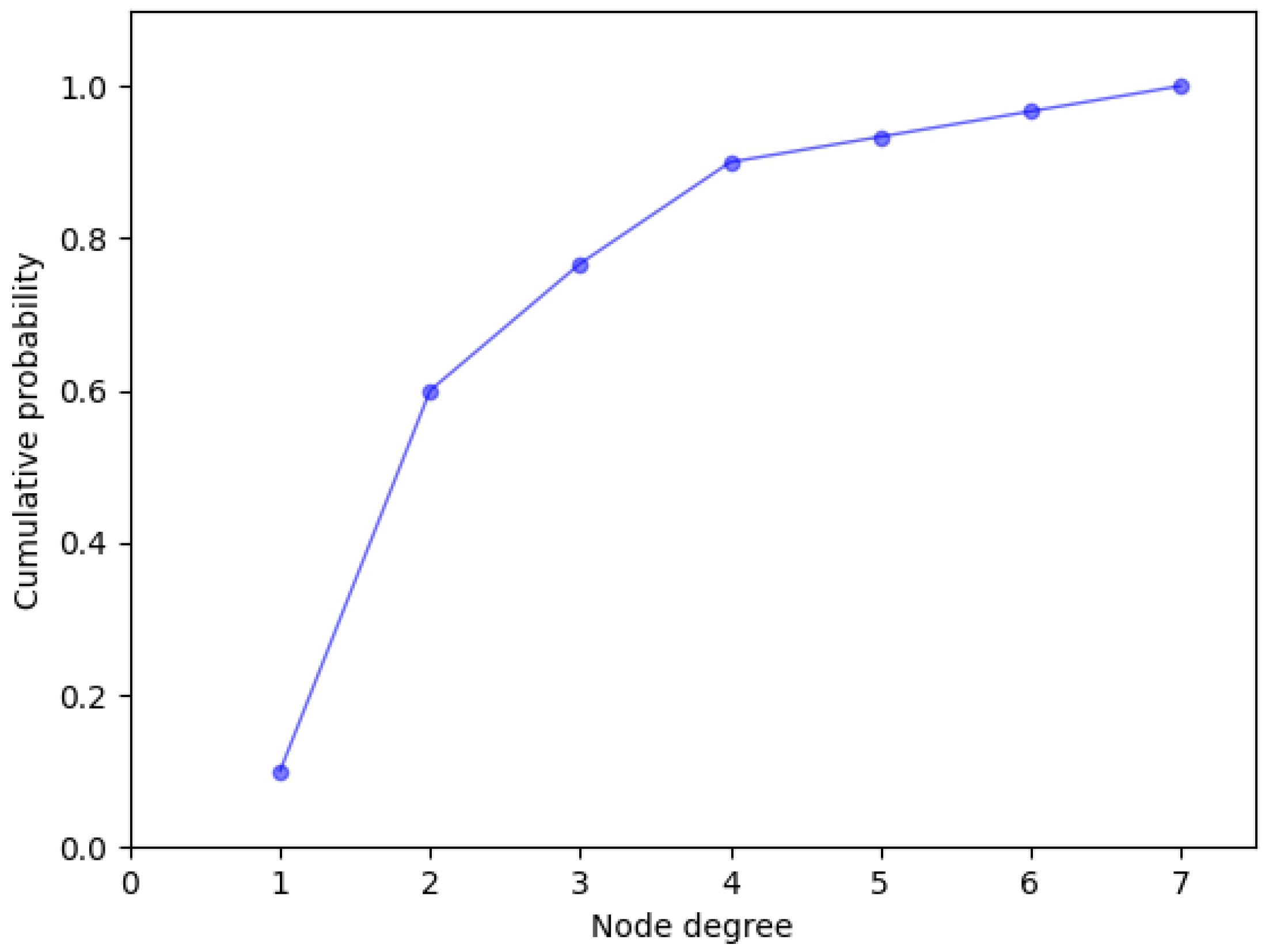
The node degree distribution is shown in Figure 8, in which the abscissa and ordinate indicate the node degree and the probability accumulation of the degree, respectively.

After traversing all nodes of the power grid in turn, the shortest path between all node pairs can be identified according to the Floyd algorithm described in Section 3. The weighted betweennesses of the node and the line are calculated according to Equations (5) and (6), respectively.

Table 8. Node weighted betweenness ranking.

Ranking	Node ID	Node Betweenness
1	6	71
2	4	38.5
3	9	37
4	10	35.5
5	12	34.5

shows the ranking of the top 5 nodes according to betweenness, and

Table 9. Line weighted betweenness ranking.

Ranking	Line ID	Line Betweenness
1	14	38
2	11	36
3	4	31
4	41	31
5	6	30
5	7	30

shows the ranking of the top 7 lines according to betweenness.

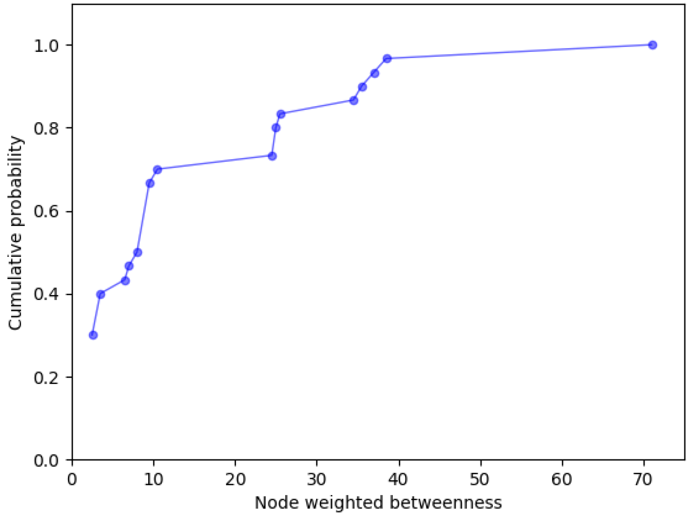
The distribution of node betweenness is shown in Figure 9. The abscissa and the ordinate are the node betweenness and the probability accumulation of the betweenness, respectively.

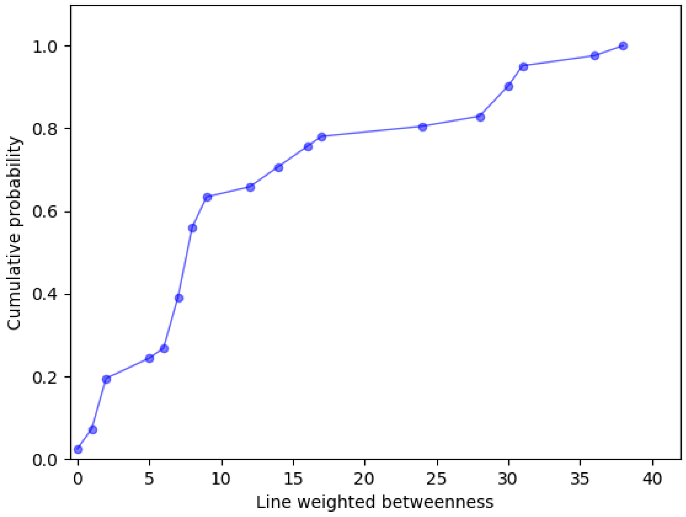
The betweenness distribution of the lines is shown in Figure 10. The abscissa and the ordinate are the line betweenness and the probability accumulation of the betweenness, respectively.

5.2. Simulation and Analysis of Power Grid Functional Vulnerability

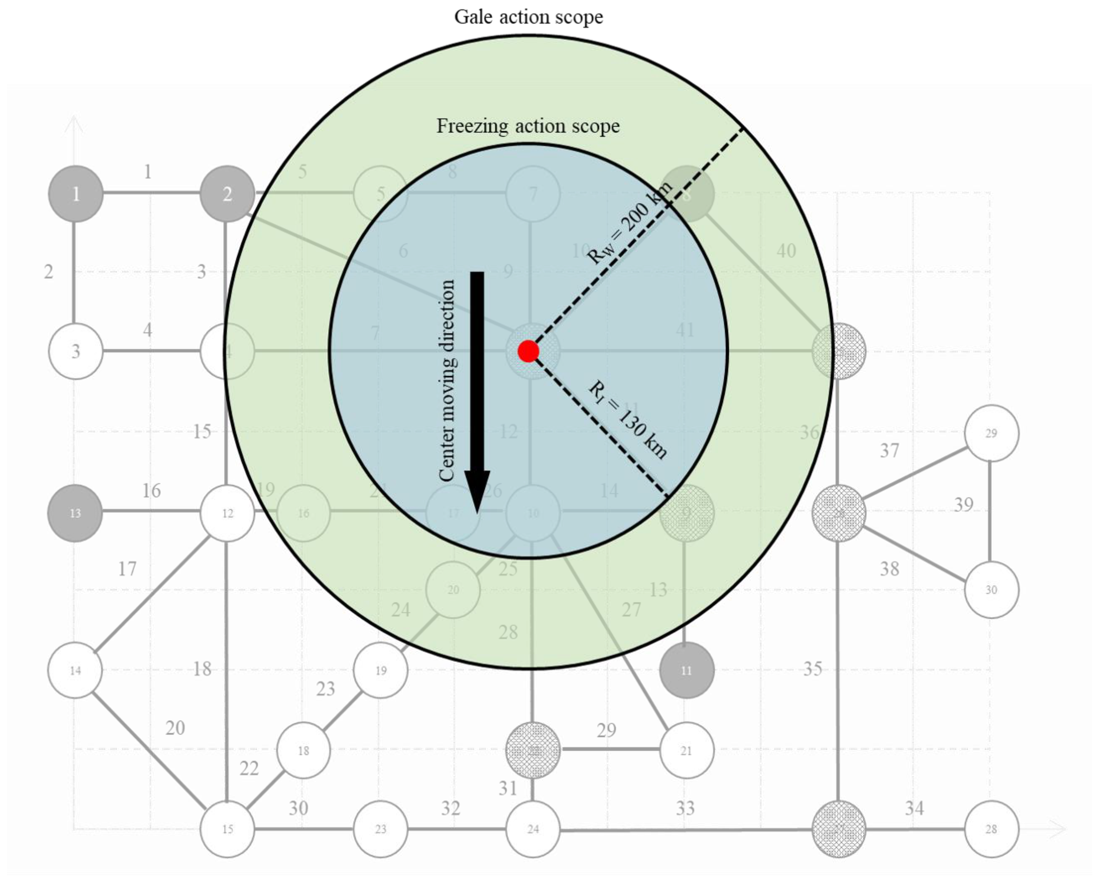
The extreme case set in this paper was severe weather with a synergistic effect of gale and freezing. The radius of the gale action was 200 km, and the radius of the freezing action was 130 km. Under the action of gale, the load calculation parameters σ_x1, σ_y1, σ_x2, and σ_y2 satisfied σ_x1 = σ_y1 = 0.4 R_W and σ_x2 = σ_y2 = 0.05 R_W; the amplitudes of severe weather A₁, A₂, and A₃ were 20 m/s, 4 m/s, and 30 mm/h, respectively; and the amplitudes of severe weather A₁, A₂, and A₃ were 25 m/s, 5 m/s, and 50 mm/h, respectively. The influence weights of the wind load a_W and the ice load a_I were 0.1 and 0.9, respectively. The initial center position of gale weather and freezing weather was (6, 10), and the center moving speed of gale weather and freezing weather was 100 km/h in the southern direction. Figure 11 shows the schematic diagram of the extreme weather scope.

5.2.1. Load Calculation

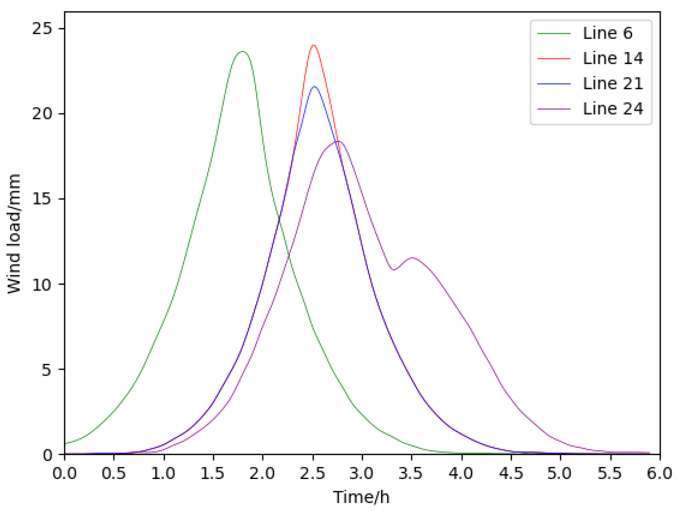
According to the computing method proposed in Section 3, the wind load and ice load of each line in the power grid under extreme weather can be obtained. The four typical lines 6, 14, 21, and 24 were selected to perform the load analysis. Figure 12 shows the wind load on these four lines.

The following could be inferred from the wind load curve:

(1)

Because of the different distances and wind direction angles between the line and the gale weather center, the wind load curve of each line was a single peak or a double peak curve.

(2)

The arrival time of the wind load extreme value was related to the relative position between the line and the beginning of the weather center. The relative positions of the four lines were different from that of the weather center, and the arrival time of wind load extreme value of these four lines also varied. Line 6 was to the north of line 14, and the distance from the initial coordinate of the weather center was shorter than that of line 14; therefore line 6 was first to be affected by the wind and reach the extreme value. Line 14 and line 21 were located at the same latitude and were almost simultaneously affected by the wind.

(3)

The extreme value of wind load was related to the distance between the line and the climate center. When the load of these four lines was at the maximum, the distance between them and the coordinates of the weather center was different. The maximum value of the wind load on line 14 and line 21 appeared nearly simultaneously, and during this time, line 14 was closer to the weather center with a larger extreme value of the wind load.

(4)

The variation trend of wind load was related to the angle between the line direction and the wind direction. Although the distance between line 21 and line 24 was close to the weather center when the wind load reached the extreme value, the angle between line 24 and the wind direction was 45°, leading to a smaller maximum value of wind load than line 21.

(5)

As the effect of wind load increased the amplitude parameter A₂, there were two maximum values on line 24 when the gale weather moved from north to south. Since the angle between line 24 and the wind direction was 45°, the two maximum values were not equal.

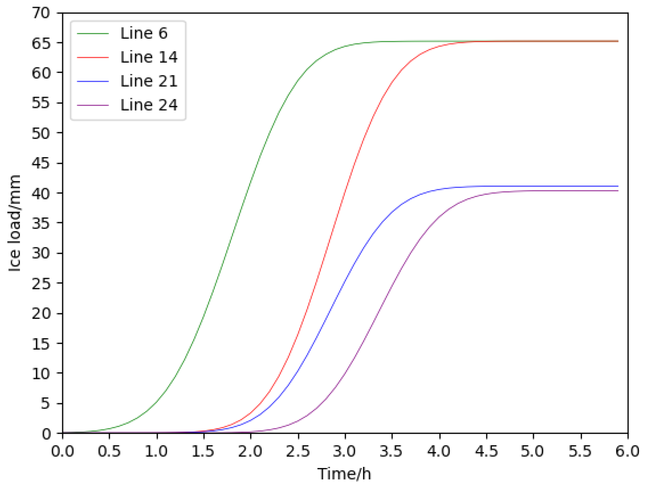
Figure 13 shows the ice load on the four lines. The following were indicated from the analysis of the ice load curve:

(1)

Since the effect of ice load on the line was cumulative, the ice load curve of each line presents S-type growth, and a moment of ice load maximum value exists, after which the ice load of the line did not increase.

(2)

The arrival time of the extreme ice load was related to the relative position between the line and the initial weather center. Line 6 was to the north of line 14, and line 21 was to the north of line 24. As a result, line 6 and line 21 were the first to be affected by the freezing weather and reach the maximum ice load.

(3)

The extreme value of the ice load was related to the distance between the line and the climate center, independent of the line. Line 14 and line 21 were the first to be affected by the maximum value of the wind load, and line 14 was closer to the weather center and bore a larger extreme value of the wind load. The distance between the maximum load point of line 6 together with line 14 and the weather center was equal, which means that the extreme value of the ice load was equal.

5.2.2. Functional Vulnerability Calculation

Based on the characteristic parameters of the power grid topology model in the previous section and the load calculated in this section, the design values dl_W and dl_i of the wind and ice loads for all lines were set to 18.95 m/s and 50 mm, respectively. The line failure rate could be obtained according to the discrete relationship between the load and line failure rates in Table 4 and Table 5. Then, the reliability of the transmission line in this extreme weather could be obtained from Equation (10). Finally, the betweenness of lines was calculated using Equation (12) to measure the functional vulnerability, and the ranking was carried out.

Table 10. Line functional vulnerability ranking based on betweenness.

Ranking	Severe Weather		Extreme Severe Weather
	Line ID	Betweenness Measuring Index	Line ID	Betweenness Measuring Index
1	6	64,868	6	249,897
2	41	60,701	41	247,462
3	7	58,743	11	243,913
4	11	51,404	7	239,479
5	14	39,229	14	209,323
6	10	22,846	10	108,406
7	28	21,110	28	97,858
8	27	14,269	27	61,105
9	12	8259	12	44,068
10	9	7226	25	38,893

shows the top 10 lines in terms of function vulnerability measured by betweenness in severe weather and extreme severe weather.

According to the index definition of power grid node functional vulnerability in Section 3, the mean reliability value of the node inflow line set and node outflow line set was calculated by Equation (15), and the influence weight of power grid node vulnerability was calculated by Equations (16)–(18). Then, the degree of nodes obtained from Equation (13) was used to measure the functional vulnerability and was ranked.

Table 11. Node function vulnerability ranking based on degree.

Ranking	Severe Weather		Extreme Severe Weather
	Node ID	Degree Measuring Index	Node ID	Degree Measuring Index
1	6	20,720	6	64,264
2	10	12,332	10	48,040
3	24	6628	22	24,946
4	22	6514	24	24,183
5	21	5235	9	21,090
6	9	5018	21	17,652
7	4	3917	4	15,966
8	7	3916	7	15,965
9	25	2938	25	11,975
9	27	2938	27	11,975

shows the top 10 lines in terms of functional vulnerability measured by the node degree in severe weather and extreme severe weather.

The node degrees obtained from Equation (14) were used to measure the functional vulnerability, and functional vulnerability was then ranked.

Table 12. Node function vulnerability ranking based on betweenness.

Ranking	Severe Weather		Extreme Severe Weather
	Node ID	Betweenness Measuring Index	Node ID	Betweenness Measuring Index
1	6	210,164	6	651,825
2	10	72,965	10	284,235
3	9	61,888	9	260,114
4	4	37,701	4	153,672
5	25	24,482	25	99,788
6	2	18,385	2	70,809
7	22	15,199	22	58,207
8	8	13,082	8	53,465
9	27	7835	23	35,806
10	7	6853	27	31,933

shows the top 10 lines of function vulnerability measured by node betweenness in severe weather and extreme severe weather.

5.2.3. Simulation Analysis

(1)

Functional vulnerability mainly reflects the difficulty of power grid units exiting the system operation due to internal causes or external interference in a short time. It can be inferred from Table 10, Table 11 and Table 12 that with increased proximity to the weather center, the power grid unit will bear a greater weather disturbance the higher the functional vulnerability. However, the units far away from the weather center are generally less vulnerable.

(2)

Table 10 shows that the vulnerability of lines in extreme severe weather is more than four times that in severe weather, while the betweenness of the lines in two extreme conditions is the same. Hence, the lines are generally vulnerable to environmental interference in extreme severe weather.

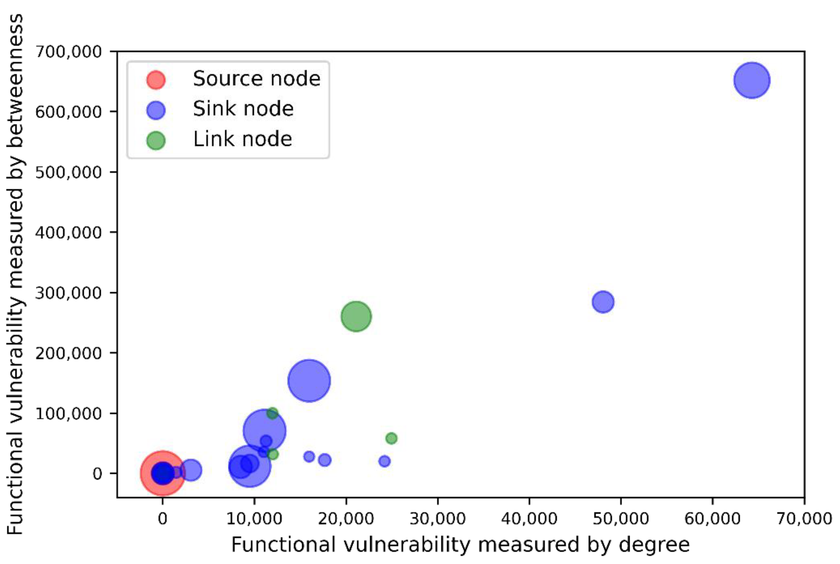
(3)

Figure 14 shows the distribution of functional vulnerability measured by degree and betweenness in extreme severe weather, of which the horizontal axis is the node degree measurement index, the vertical axis is the node betweenness measurement index, and the area of scattered points is the grid betweenness. As shown in Figure 14, there is a linear positive correlation between the node degree measuring index and the betweenness measuring index. The degree measuring index considers the influence of the node on its neighborhood, and the betweenness measuring index considers the overall influence of the node on the power grid system.

(4)

In the normal case, the nodes with high characteristic parameters in the topology model are not guaranteed to have a higher functional vulnerability and vice versa. For instance, nodes 10 and node 25 have lower betweenness in the normal case, but their functional vulnerability is high. Therefore, the nodes that need to be protected and monitored are those with high functional vulnerability, not those with high betweenness.

6. Conclusions

In this paper, the topology of the power grid was modeled based on the complex network theory, which considers the impact of extreme weather on power grid and researches the functional vulnerability of the power grid. The main contributions of this paper are as follows: a topology model of the power grid based on complex network modeling was constructed; a functional vulnerability model based on reliability was established; and the proposed model was verified through a simulation experiment.

The major conclusions are as follows:

(1)

A power grid topology model based on complex network modeling was constructed. According to the relationship between output power and load power, the nodes were divided into source nodes, sink nodes, and link nodes, and the undirected topology model was transformed into a directed topology model according to node voltage. By introducing the line reactance, the weighted model was transformed into the weighted model, which can better identify the vulnerability of different units. In addition, the node degree, node weighted betweenness, and line weighted betweenness were defined as the characteristic parameters of the power grid topology model to analyze its topology characteristics.

(2)

A functional vulnerability model based on reliability was established. The reliability of the line was obtained by calculating the load in gale weather, freezing weather, and freezing gale weather. The functional vulnerability of the line was calculated by weighting the line reliability with the line betweenness. The node functional vulnerability weight was defined by the line reliability of the node neighborhood, and then the node functional vulnerability model measured by degree and betweenness was obtained based on the above work.

(3)

The model and algorithm proposed in this paper were verified by a simulation experiment. Taking the IEEE-30 bus system as an example, the topology model of power grid system was established to simulate the load and vulnerability of the power grid in freezing and gale weather. The power grid functional vulnerability level under different units and modes was analyzed to put forward suggestions on the maintenance of the power grid, which was verified through the simulation experiment. The simulation results show that the vulnerability of the power grid unit reaches the highest value under the synergistic effect of extreme weather.

References

- Hu, X.; Tang, W.; Liu, H.; Zhang, D.; Lian, S.; He, Y. Construction of bulk power grid security defense system under the background of AC/DC hybrid EHV transmission system and new energy. In Proceedings of the IECON 2017-43rd Annual Conference of the IEEE Industrial Electronics Society, Beijing, China, 29 October–1 November 2017; IEEE: Piscataway, NJ, USA, 2017; pp. 5713–5719. [Google Scholar]
- Wang, D.; Hu, T.; Zhang, J.; Mei, Y.; Zhang, B.; Wang, H.; Xu, J.; Peng, C.; Peng, G. Studying the SVC Control Strategy of the Ali Interconnection Project. In Proceedings of the 2020 IEEE Sustainable Power and Energy Conference (iSPEC), Chengdu, China, 23–25 November 2020; IEEE: Piscataway, NJ, USA, 2020; pp. 1064–1069. [Google Scholar]
- Chen, Y. Analysis on defence plan of cascading failures in CSG in dispatcher’s perspective. In Proceedings of the 2011 International Conference on Advanced Power System Automation and Protection, Beijing, China, 16–20 October 2011; IEEE: Piscataway, NJ, USA, 2011; Volume 2, pp. 1100–1103. [Google Scholar]
- Li, D.; Gong, Y.; Shen, S.; Feng, G. Research and Design of Meteorological Disaster Early Warning System for Power Grid Based on Big Data Technology. In Proceedings of the 2020 Asia Energy and Electrical Engineering Symposium (AEEES), Chengdu, China, 29–31 May 2020; IEEE: Piscataway, NJ, USA, 2020; pp. 658–662. [Google Scholar]
- Billonton, R.; Acharya, J.R. Weather-Based Distribution System Reliability Evaluation. IEE Proc. Gener. Transm. Distrib. 2006, 153, 499–506. [Google Scholar] [CrossRef]
- Johnson, C.W. Analysing the causes of the italian and swiss blackout, 28th september 2003. In Proceedings of the 12th Australian Workshop on Safety Critical Systems and Software-Related Programmable Systems, Adelaide, Australia, 30–31 August 2007; pp. 21–30. [Google Scholar]
- Bo, Z.; Shaojie, O.; Jianhua, Z.; Hui, S.; Geng, W.; Ming, Z. An analysis of previous blackouts in the world: Lessons for China’s power industry. Renew. Sustain. Energy Rev. 2015, 42, 1151–1163. [Google Scholar] [CrossRef]
- Van Der Bruggen, K. Critical infrastructures and responsibility: A conceptual exploration. Safety Sci. 2008, 46, 1137–1148. [Google Scholar] [CrossRef]
- Li, T.; Li, J. Analysis of icing accident in South China power grids in 2008 and it’s countermeasures. In Proceedings of the CIRED 2009-20th International Conference and Exhibition on Electricity Distribution-Part 1, Prague, Czech Republic, 8–11 June 2009; IET: London, UK, 2009; pp. 1–4. [Google Scholar]
- Matthewman, S.; Byrd, H. Blackouts: A sociology of electrical power failure. Social Space Przestrzeń Społeczna 2013, 2, 31–55. [Google Scholar]
- Lucas, A. Confected conflict in the wake of the South Australian blackout: Diversionary strategies and policy failure in Australia’s energy sector. Energy Res. Soc. Sci. 2017, 29, s149–s159. [Google Scholar] [CrossRef]
- Sun, H.; Xu, T.; Guo, Q.; Li, Y.L.; Lin, W.F. Analysis on blackout in Great Britain power grid on 9th August, 2019 and its enlightenment to power grid in China. In Proceedings of the CSEE, Beijing, China, 6–8 March 2019; Volume 39, pp. 6183–6191. [Google Scholar]
- Wang, Y.; Wu, J.; Yi, H. Analysis on Several Blackouts Caused by Extreme Weather and its Enlightenment. In IOP Conference Series: Earth and Environmental Science; IOP Publishing: Chengdu, China, 2021; Volume 766, p. 012020. [Google Scholar]
- Watts, D.J.; Strogatzs, H. Collective Dynamics of small-world Networks. Nature 1998, 393, 440–442. [Google Scholar] [CrossRef]
- Watts D, J. Small-worlds: The dynamics of between order and randomness. Am. Math. Mon. 2000, 107, 664–668. [Google Scholar] [CrossRef]
- Surdutovich, G.; Cortez, C.; Vitilina, R.; Da Silva, J.P. Dynamics of “small world” networks and vulnerability of the electric power grid. In Proceedings of the VIII Symposium of Specialists in Electric Operational and Expansion Planning, Brasilia, Brazil, 19–23 May 2002; pp. 112–116. [Google Scholar]
- Sperstad, I.B.; Kjølle, G.H.; Gjerde, O. A comprehensive framework for vulnerability analysis of extraordinary events in power systems. Reliab. Eng. Syst. Saf. 2020, 196, 106788. [Google Scholar] [CrossRef]
- Fouad, A.A.; Zhou, Q.; Vittal, V. System vulnerability as a concept to assess power system dynamic security. IEEE Trans. Power Syst. 1994, 9, 1009–1015. [Google Scholar] [CrossRef]
- Bompard, E.; Napoli, R.; Xue, F. Extended topological approach for the assessment of structural vulnerability in transmission networks. IET Gener. Transm. Distrib. 2010, 4, 716–724. [Google Scholar] [CrossRef]
- Cadini, F.; Agliardi, G.L.; Zio, E. A modeling and simulation framework for the reliability/availability assessment of a power transmission grid subject to cascading failures under extreme weather conditions. Appl. Energy 2017, 185, 267–279. [Google Scholar] [CrossRef] [Green Version]
- Zhou, T.; Lu, J.; Li, B.; Tan, Y. Fractal analysis of power grid faults and cross correlation for the faults and meteorological factors. IEEE Access 2020, 8, 79935–79946. [Google Scholar] [CrossRef]
- Billinton, R.; Bollinger, K.E. Transmission System Reliability Evaluation using Markov Processes. IEEE Trans. Power App. Syst. 1968, 87, 538–547. [Google Scholar] [CrossRef]
- Billinton, R.; Singh, G. Application of adverse and extreme adverse weather: Modelling in transmission and distribution system reliability evaluation. IEE Proc. Gener. Transm. Distrib. 2006, 153, 115–120. [Google Scholar] [CrossRef]
- Alvehag, K.; Soder, L. A Stochastic Weather Dependent Reliability Model for Distribution Systems. In Proceedings of the 10th International Conference on Probabilistic Methods Applied to Power Systems, Rincon, PR, USA, 25–29 May 2008; pp. 1–8. [Google Scholar]
- Alvehag, K.; Soder, L. A Reliability Model for Distribution Systems Incorporating Seasonal Variations in Severe Weather. IEEE Trans. Power Deliv. 2011, 26, 910–919. [Google Scholar] [CrossRef]
- Brostrom, E.; Ahlberg, J.; Soder, L. Modelling of Ice Storms and their lmpact Applied to a Part of the Swedish Transmission Network. In 2007 IEEE Lausanne Power Tech, Lausanne, Switzerland, 1–5 July 2007; IEEE: Piscataway, NJ, USA, 2007; pp. 1593–1598. [Google Scholar]
- Ju, Y.Z.; Xue, Q.L.; Li, H. Failure Analysis of Transmission Tower under the Effect of Ice-Covered Power Transmission Line. Proceedings of 1st International Conference on Information Science and Engineering (ICISE), Nanjing, China, 26–28 December 2009; pp. 4301–4304. [Google Scholar]
- Makkonen, L. Models for the growth of rime, glaze, icicles and wet snow on structures. Philos. Trans. Royal Soc. Lond. Ser. A Math. Phys. Eng. Sci. 2000, 358, 2913–2939. [Google Scholar] [CrossRef]
- Jiang, X.; Bi, M.; Hu, J.; Zhang, Z.; Xia, Y. Influence of test methods on dc flashover performance of ice-covered composite insulators and statistical analysis. IEEE Trans. Dielectr. Electr. Insul. 2012, 19, 2019–2028. [Google Scholar] [CrossRef]
- Goodwin, E.J., III; Mozer, J.D.; DiGioia, A.M., Jr.; Power, B.A. Predictingice and Snowloads for Transmission Line Design; Pennsylvania Power and Light Co.: Allentown, PA, USA, 1982; pp. 267–273. [Google Scholar]
- Liu, Y.; Singh, C. A Methodology for Evaluation of Hurricane Impact on Composite Power System Reliability. IEEE Trans. Power Syst. 2011, 26, 20–25. [Google Scholar] [CrossRef]
- Bhuiyan, M.R.; Allan, R.N. Inclusion of weather effects in composite system reliability evaluation using sequential simulation. IEE Proc. Gener. Transm. Distrib. 1994, 141, 575–584. [Google Scholar] [CrossRef]
- Kiel, E.S.; Kjølle, G.H. The impact of protection system failures and weather exposure on power system reliability. In Proceedings of the 2019 IEEE International Conference on Environment and Electrical Engineering and 2019 IEEE Industrial and Commercial Power Systems Europe (EEEIC/I&CPS Europe), Genova, Italy, 11–14 June 2019; IEEE: Piscataway, NJ, USA, 2019; pp. 1–6. [Google Scholar]
- Wang, Y.; Rousis, A.O.; Strbac, G. On microgrids and resilience: A comprehensive review on modeling and operational strategies. Renew. Sustain. Energy Rev. 2020, 134, 110313. [Google Scholar] [CrossRef]
- Nguyen, H.T.; Muhs, J.; Parvania, M. Preparatory operation of automated distribution systems for resilience enhancement of critical loads. IEEE Trans. Power Deliv. 2020, 36, 2354–2362. [Google Scholar] [CrossRef]
- Zhou, J.; Zhao, W.; Zhang, S.; Liu, Y.; Gong, J.; Ye, Y. Resilience Enhancement of Power Grid Considering Optimal Operation of Regional Integrated Energy System Under Typhoon Disaster. In Proceedings of the 2021 3rd Asia Energy and Electrical Engineering Symposium (AEEES), Chengdu, China, 26–29 March 2021; IEEE: Piscataway, NJ, USA, 2021; pp. 546–551. [Google Scholar]
- Hou, H.; Yu, S.; Wang, H.; Xu, Y.; Xiao, X.; Huang, Y.; Wu, X. A hybrid prediction model for damage warning of power transmission line under typhoon disaster. IEEE Access 2020, 8, 85038–85050. [Google Scholar] [CrossRef]
- Karangelos, E.; Perkin, S.; Wehenkel, L. Probabilistic Resilience Analysis of the Icelandic Power System under Extreme Weather. Appl. Sci. 2020, 10, 5089. [Google Scholar] [CrossRef]
- Jufri, F.H.; Widiputra, V.; Jung, J. State-of-the-art review on power grid resilience to extreme weather events: Definitions, frameworks, quantitative assessment methodologies, and enhancement strategies. Appl. Energy 2019, 239, 1049–1065. [Google Scholar] [CrossRef]
- Mousavizadeh, S.; Bolandi, T.G.; Haghifam, M.R.; Moghimi, M.; Lu, J. Resiliency analysis of electric distribution networks: A new approach based on modularity concept. Int. J. Electr. Power Energy Syst. 2020, 117, 105669. [Google Scholar] [CrossRef]
- Amja, N.; Esmaili, M. Improving voltage security assessment and ranking vulnerable buses with consideration of power system limits. Electr. Power Energy Syst. 2003, 25, 705–715. [Google Scholar] [CrossRef]
- Ubeda, J.R.; Allan, R.N. Sequential simulation applied to composite system reliability evaluation. IEEE Trans. Power Syst. 1994, 9, 81–86. [Google Scholar] [CrossRef]
- Singh, C.; Patton, A.D. Protection system reliability modeling: Unreadiness probability and Mean duration of undetected faults. IEEE Trans. Power Syst. 1980, 29, 339–340. [Google Scholar] [CrossRef]
- Xingbin, Y.; Singh, C. A practical approach for integrated power system vulnerability analysis with protection failures. IEEE Trans. Power Syst. 2004, 19, 1818–1820. [Google Scholar]
- Sheng, S.; Li, K.K.; Chan, W.L.; Xiangjun, Z.; Xianzhong, D. Monte Carlo based maintenance resource allocation considering vulnerability. In Proceedings of the Transmissionand Distribution Conference & Exhibition: Asia and Pacific, Dalian, China, 18 August 2005. [Google Scholar]
- Nan, L.; Wu, L.; Liu, T.; Liu, Y.; He, C. Vulnerability identification and evaluation of interdependent natural gas-electricity systems. IEEE Trans. Smart Grid 2020, 11, 3558–3569. [Google Scholar] [CrossRef]
- Liu, Y.; Wotherspoon, L.; Nair, N.K.C.; Blake, D. Quantifying the seismic risk for electric power distribution systems. Struct. Infrastruct. Eng. 2021, 17, 217–232. [Google Scholar] [CrossRef]
- Abedi, A.; Gaudard, L.; Romerio, F. Power flow-based approaches to assess vulnerability, reliability, and contingency of the power systems: The benefits and limitations. Reliab. Eng. Syst. Saf. 2020, 201, 106961. [Google Scholar] [CrossRef]
- Fang, J.; Wu, J.; Zheng, Z.; Chi, K.T. Revealing structural and functional vulnerability of power grids to cascading failures. IEEE J. Emerg. Sel. Top. Circuits Syst. 2020, 11, 133–143. [Google Scholar] [CrossRef]
- Xie, X.; Ma, D.; Na, Z.; Lu, Y.; Luo, X. Improvement strategy for robustness of power grid complex network by distributed photovoltaic power system. In Proceedings of the E3S Web of Conferences, Divnomorskoe, Russian, 4 December 2019; EDP Sciences: Les Ulis, France, 2020; Volume 143, p. 02019. [Google Scholar]
- Xiao, S.; Zhang, J. Assessment of power grid vulnerability based on small-world topological model. Power Syst. Technol. 2010, 34, 64–68. [Google Scholar]
- Ding, M.; Han, P. Vulnerability assessment to small-world power grid based on weighted topological model. Proc. Chin. Soc. Electr. Eng. Chin. Soc. Electr. Eng. 2008, 28, 20. [Google Scholar]
- Zhenbo, W.; Junyong, L.; Guojun, Z. Vulnerability evaluation model to power grid based on reliability-parameter-weighted topological model. Trans. China Electrotech. Soc. 2010, 25, 131–137. [Google Scholar]
- Zhang, R.; Du, Y.; Yuhong, L. New challenges to power system planning and operation of smart grid development in China. In Proceedings of the 2010 International Conference on Power System Technology, Hangzhou, China, 24–28 October 2010; IEEE: Piscataway, NJ, USA, 2010; pp. 1–8. [Google Scholar]
- Li, G.; Zhang, P.; Luh P, B.; Li, W.; Bie, Z.; Serna, C.; Zhao, Z. Risk analysis for distribution systems in the northeast US under wind storms. IEEE Trans. Power Syst. 2012, 29, 889–898. [Google Scholar] [CrossRef]
- Chen, X.; Qiu, J.; Reedman, L.; Dong, Z.Y. A statistical risk assessment framework for distribution network resilience. IEEE Trans. Power Syst. 2019, 34, 4773–4783. [Google Scholar] [CrossRef]
- Chen, X. An Optimal Trading Mechanism to Address Network Resiliency in a Distribution Electricity Market with High Renewable Penetration. Ph.D. Thesis, the University of New South Wales, Sydney, Australia, 2020. [Google Scholar]
- Alexandersson, H.; Tuomenvirta, H.; Schmith, T.; Iden, K. Trends of storms in NW Europe derived from an updated pressure data set. Clim. Res. 2000, 14, 71–73. [Google Scholar] [CrossRef] [Green Version]
- Brostrom, E.; Soder, L. Modeling of Ice Storms for Power Transmission reliabilit Calculations. In Proceedings of the 15th Power Systems Computation Conference, Liege, Beigium, 22–26 August 2005; p. 7. [Google Scholar]
- Juanjuan, W.; Chuang, F.; Yiping, C.; Hong, R.; Shukai, X.; Tao, Y.; Licheng, L. Research and application of DC de–icing technology in China southern power grid. IEEE Trans. Power Deliv. 2012, 27, 1234–1242.3. [Google Scholar] [CrossRef]
- Liu, J.; Liu, Y.; Zhang, L.; Yang, D.; Wang, H.; Jiang, F. Gale Change and Grading for Power Grid Wind Zone in Jiangsu Province. In Proceedings of the 2019 IEEE 3rd Conference on Energy Internet and Energy System Integration (EI2), Changsha, China, 8–10 November 2019; IEEE: Piscataway, NJ, USA, 2019; pp. 2413–2417. [Google Scholar]
- Sinha, A.A.; Arya, M.K.; Kumar, A.; Mandal, R.K.; Biswas, M.; Ghosh, B.K.; Roy, S. Linear sensitivity based congestion management of IEEE 30 bus system using distributed generator. In Proceedings of the 2018 2nd International Conference on Trends in Electronics and Informatics (ICOEI), Tirunelveli, India, 11–12 May 2018; IEEE: Piscataway, NJ, USA, 2018; pp. 691–696. [Google Scholar]
Figure 1.
The framework of the proposed method.
Figure 2.
Virtual node diagram; (a,b) represent the source node and sink node, respectively.
Figure 3.
Flow chart of power grid topology modeling and characteristic parameter analysis.
Figure 4.
Diagram of the relative position between the line and the weather center as well as the wind load action.
Figure 5.
Flow chart of the power grid functional vulnerability analysis.
Figure 6.
IEEE-30 system wiring diagram [62].
Figure 7.
IEEE-30 system topology model diagram.
Figure 8.
Node degree distribution of the IEEE-30 bus system.
Figure 9.
Node betweenness distribution of the IEEE-30 bus system.
Figure 10.
Line betweenness distribution of the IEEE-30 bus system.
Figure 11.
Schematic diagram of the extreme weather action scope.
Figure 12.
Wind load curve for representative lines.
Figure 13.
Ice load curve for representative lines.
Figure 14.
Functional vulnerability distribution of power grid nodes measured by degree and betweenness.