Air-Gap Flux Oriented Vector Control Based on Reduced-Order Flux Observer for EESM

Abstract

Electrically excited synchronous motor (EESM) has the characteristics of high order, nonlinear and strong coupling, so it is difficult to be controlled. However, it has the advantages of adjustable power factor, high efficiency, and high precision torque control, so it is widely used in high-power applications. The accuracy of a flux observer influences the speed control system of EESM. Based on state observer in modern control theory and electrical excitation synchronous machine state equation, a reduced-order flux observer is designed. Using the first-order difference method and forward bilinear transformation method, the reduced-order flux observer is discrete, and the stability of the motor system is analyzed. The analysis shows that the stability of the system using the bilinear transformation method is better than that using the first order forward difference method. In motor operation, motor parameters will be affected by the factors of temperature, magnetic saturation, and motor frequency. In this paper, the influence of parameter variation on the motor system is studied by using the variation of the pole distribution. Finally, the speed regulation system using the reduced-order observer is simulated, which verifies the accuracy of the reduced-order flux observer observation.

1. Introduction

With the continuous development of the world economy, the problem of energy consumption has attracted extensive attention from scholars [1,2,3]. In the face of severe energy consumption and environmental pollution, it is urgent to seek ways to improve energy utilization. In the modern industry, the loss of energy of the motor occupies a large proportion, and the optimization of the motor speed regulation system has a great impact on energy saving. In the field of electric drive, DC motor drive and AC motor drive are two main types [4,5,6,7,8]. DC motor drive developed earlier, and its simple control and better speed regulation performance make its research relatively mature. However, due to the limitation of the DC motor brush and commutator, it is difficult to make a big breakthrough in high-power drive. Compared with the DC motor, the AC motor can avoid the limitation of power, but its control method developed slowly until the coordinate transformation theory and vector control theory were put forward in the mid-20th century, and the control theory research of the AC motor began to develop rapidly. The coordinate transformation theory and vector control theory unify AC motor control and DC motor control. With the maturity of vector control, the control performance of the AC motor has also been improved, and the application range is more and more extensive. In the AC motor, the synchronous motor has the advantages of high-power factor and small moment of inertia, so it is widely used in high-power occasions and high-performance speed regulation fields [9,10,11].

The synchronous motor mainly includes the electric excitation synchronous motor and the permanent magnet synchronous motor. The difference between the two is that the rotor magnetic field of the permanent magnet synchronous motor is provided by the permanent magnet, while the rotor magnetic field of the electric excitation synchronous motor is provided by the field winding, which can adjust the size of the excitation current. Currently, with the research of the rotor excitation structure of electric synchronous motor, the traditional brush excitation structure has been improved accordingly [12,13,14,15]. An electrically excited synchronous motor has the characteristics of high-order nonlinear strong coupling, so it is difficult to control but its power factor adjustable efficiency and high torque control precision make it widely used in high-power occasions, such as mine hoist rolling mills.

The vector control system began in the middle of the 20th century. The vector control theory is mainly based on the control principle of induction motor field orientation published by F. Brazchke and other scholars of Siemens in Germany and the coordinate transformation control of induction motor stator voltage applied by P.C.Custman and A.A. Clarke in the United States established by the patent. In recent years, domestic and foreign scholars have conducted a lot of research on the vector control of AC-DC-AC synchronous motors, and large foreign companies, such as Siemens, ABB and Toshiba, have mastered most of the core technologies [16,17,18]. In the vector control system, scholars have conducted a lot of work to improve the performance of vector control systems; these are mainly studies of the decoupling for the vector control system, the improvement of the regulator on the vector control system, the angle of the closed-loop and magnetic chain saturated. Direct torque control (DTC) was first proposed by Professor M. Depenbrock from Ruhr University in Germany and Japanese scholar I. Takahashi in 1985, which has aroused extensive attention and research in the academic world. At that time, DTC was put forward mainly for asynchronous motors, and it was not until 1998 that some scholars applied DTC to electrically excited synchronous motors. The torque control system directly controls the torque and flux [19]. The traditional method is bang-bang control. In this method, the torque and flux are transferred through the hysteresis comparator, respectively, to determine the voltage vector switching state. The advantages of the traditional method include simple control structure, fast torque dynamic response, low parameter sensitivity and no need for rotation coordinate transformation, etc., and disadvantages include low-speed torque observation error, large flux observation error, large current pulsation, etc. Therefore, there is still a great distance from the actual production and application. Because of the defects in the traditional direct torque control system, scholars put forward many schemes to improve them. The SVM-DTC control method is a good solution to the problems in traditional methods [20,21,22]. This method is mainly produced by the combination of the space vector pulse width modulation (SVPWM) strategy and direct torque control. With the improvement of the direct torque control method, more and more industrial applications have seen the figure of direct torque control.

The control strategies based on modern control theories include robust observer, model reference adaptive and sliding mode variable structure control, etc. These theories have been used in motor control systems. Model reference adaptive control (MRAS) is widely used in sensorless motors [23,24,25,26]. Sliding mode control (SMC) as a hot spot in the variable structure control is mainly used to replace the traditional PI regulator and has been gradually applied in the field of motor control. The main disadvantages of modern control theory are as follows: it is highly dependent on the mathematical model of the motor and requires high sampling accuracy [27,28,29,30,31,32,33,34,35,36]. Therefore, it requires many sensors with high accuracy for accurate observation. Moreover, most modern control theories are based on linear systems, and their robustness is poor, so there is much room for improvement [37]. As discussed in above, lots of research has been conducted and many high-quality control schemes are applied to the control of permanent magnet motors, thus

Table 1. Advantages and disadvantages of different control schemes for EESM.

Control Scheme	Advantages	Disadvantages
Direct torque control	No coordinate transformation and current control; simple structure	Torque and flux ripple;
Model reference adaptive control	Adjustable controller parameters; independent of the controlled object; strong fault tolerance	Difficult to prove stability; convergence analysis method lacks universality; unclear robustness
Sliding mode control	Fast response; simple algorithm; strong robustness	Chattering in the dead zone; long approach time

shows the main advantages and disadvantages of the described control techniques.

In the electrical excitation synchronous motor (EESM) speed control system, regardless of vector control and direct torque control, it is needed to obtain accurate information about the magnetic chain. The commonly used method is to construct a flux observer of flux linkage amplitude and flux linkage angle. The flux observer design of electric excitation synchronous motor speed control system has a great influence [38,39,40]. The improvement of the flux observer can better improve the performance of the speed regulation system. The working principle of the current model flux observer is to observe the flux by solving the magnetization current of the motor current. This kind of flux observation model is sensitive to the motor parameters and requires a higher accuracy of current sampling. When the motor is running, the parameters of the motor tend to change with the change of temperature [41,42,43]. Therefore, when the motor is running at medium and high speed, the observed value of the current model for the flux linkage will deviate greatly from the actual value. At the same time, the current model uses the approximate demagnetization curve to solve the flux, but the influence of flux saturation in the actual operation will also lead to the deviation of observation. In addition, the current model is based on the steady-state of the motor, and the influence of the transient component of the motor on the observer is not considered. The voltage model flux observer obtains the flux by integrating the back electromotive force. The initial value of the integral and the accumulated errors of the integral will affect the flux observation results. The observation deviation of the universal voltage model flux observer is obvious at low speed, because the stator voltage is small at low speeds, and the stator resistance has the effect of voltage division. By combining the equation of the state of the motor with the design method of the state observer in modern control theory, the motor flux can be observed [44]. The state observer can be divided into full-order observer and reduced-order observer, which has been applied in the flux observation of induction motor and sensorless control of permanent magnet synchronous motor [45].

In this paper, the flux observer of the electrically excited synchronous motor is studied, and the reduced-order flux observer of the electrically excited synchronous motor is designed based on modern control theory. The influence of different discretization methods on the stability of the motor control system is analyzed. The first-order forward difference method and bilinear transformation method are used to discretize the reduced-order flux observer, and the influence of the change of motor parameters on the stability of the motor system is analyzed. The voltage parameters of the reduced-order flux observer are obtained by voltage reconstruction of the frequency converter, and the simulation and experimental analysis of the reduced-order flux observer are carried out.

The paper is organized as follows. First, the mathematical model of EESM is presented in Section 2. Section 3 describes the design and discretization of the reduced-order flux observer of EESM. The simulation results are presented in Section 4. Finally, the conclusion is given in Section 5.

2. Mathematical Model of EESM

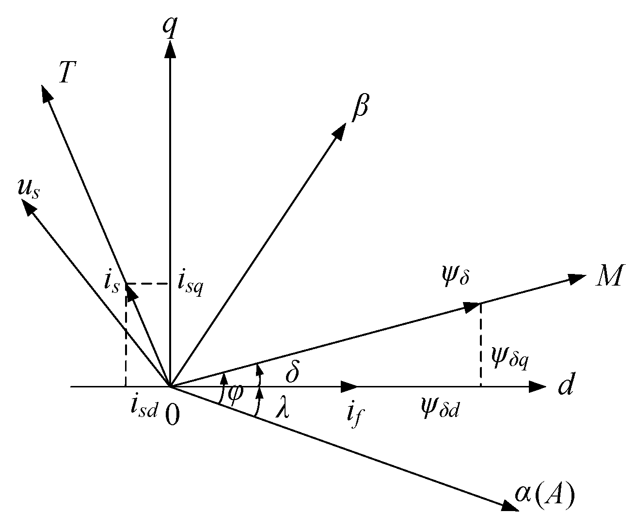
Figure 1 shows the commonly used coordinate systems for EESM, namely, the three-phase static coordinate system, the two-phase static αβ coordinate system, the two-phase rotating dq coordinate system and the magnetic field oriented two-phase rotation MT coordinate system. The axis coincident with the stator winding A is defined as the α axis, while the coordinate axis coincidentally with the rotor axis is defined as the d axis and the coordinate axis coincident with the flux ψ_δ is defined as the M axis.

The included angle between axis d and axis α is the rotor position angle λ, the included angle between axis M and axis α. φ is the flux linkage angle, and the included angle between axis M and axis d. δ is called the load angle.

The meaning of symbols used in following equations are listed in

Table 2. Symbols list.

Symbol	Meaning
ψdq	The flux of dq axis
Ldq Idq	The synchronous inductance of dq axis the current of dq axis
Udq	The voltage of dq axis
Rdq	The resistance of dq axis
ωr	The speed of rotor
TL	The load torque

.

The mathematical expression of the electrically excited synchronous motor in the coordinate system of dq axis is:

• Mathematical expression for flux linkage
  $${\left[\psi \right]}_{dq}={\left[L\right]}_{dq}{[I]}_{dq}$$

  (1)

  where the flux matrix, current matrix and inductance matrix in the coordinate system of dq axis are, respectively: ${\left[\psi \right]}_{dq}=\left[{\psi }_{sd} {\psi }_{sq} {\psi }_f {\psi }_{Dd} {\psi }_{Dq}\right]$, ${\left[I\right]}_{dq}=\left[i_{sd} i_{sq} i_f i_{Dd} i_{Dq}\right]$, ${\left[L\right]}_{dq}=\left[\begin{array}{ccccc}{L}_d& 0& L_{ad}& L_{ad}& 0\\ 0& L_q& 0& 0& L_{aq}\\ L_{ad}& 0& L_f& L_{ad}& 0\\ L_{ad}& 0& L_{ad}& L_{Dd}& 0\\ 0& L_{aq}& 0& 0& L_{Dq}\end{array}\right]$, where L_ad, L_aq are, respectively, the dq axis armature reaction inductance, L_d L_q are the synchronous inductance of dq axis, L_f is the rotor excitation winding self-induction, L_Dd and L_Dq are the self-induction of the damping winding dq axis; the relationship between inductors can be expressed as follows:

  $$\{\begin{array}{l}{L}_d=L_{ad}+L_{sl}\\ L_q=L_{aq}+L_{sl}\\ L_f=L_{ad}+L_{fl}\\ L_{Dd}=L_{ad}+L_{Ddl}\\ L_{Dq}=L_{aq}+L_{Dql}\end{array}$$

  (2)

  where L_sl and L_fl are the leakage inductance of stator winding and rotor excitation winding, L_Ddl and L_Dql are the leakage inductance of the damping winding dq axis.
• Mathematical expression of voltage
  $${\left[U\right]}_{dq}={[R]}_{dq}{[I]}_{dq}+p{[\psi ]}_{dq}+{\omega }_r\left[D\right]{[\psi ]}_{dq}$$

  (3)

  where the voltage matrix, resistance matrix and D matrix are, respectively: ${\left[U\right]}_{dq}={\left[u_{sd} u_{sq} u_f 0 0\right]}^T$, ${\left[R\right]}_{dq}=\left[R_s R_s R_f R_{Dd} R_{Dq}\right]$, $\left[D\right]=\left[\begin{array}{ccccc}0& -1& 0& 0& 0\\ 1& 0& 0& 0& 0\\ 0& 0& 0& 0& 0\\ 0& 0& 0& 0& 0\\ 0& 0& 0& 0& 0\end{array}\right]$.
• Mathematical expression of electromagnetic torque

  $$T_e=p_n({\psi }_{sd}{i}_{sq}-{\psi }_{sq}{i}_{sd})$$

  (4)

  where p_n is the pole logarithm of EESM.
• The expression between electromechanical magnetic torque, load torque and speed is as follows:

  $$T_e-T_L=J\frac{d{\omega }_r}{dt}$$

  (5)

3. Design and Discretization of Reduced-Order Flux Observer of EESM

Flux observer is used to observing the flux amplitude and flux angle in the speed regulation system of EESM. The quality of flux observation will directly affect the performance of the motor speed regulation system. Due to the existence of excitation winding and damping winding, the state equation of EESM is complicated. To simplify the design of state observers, a reduced-order flux observer can be designed according to the reduced-order observer design method. When using different discretization algorithms to discretize the reduced-order flux observer, the stability conditions are also different. Since the state observer is based on the state equation of the motor, it depends very much on the parameters of the motor, so this paper analyzes the stability of the speed regulation system of the electric excitation synchronous motor under the change of the parameters of the motor.

3.1. Equation of State for EESM

Since the reduced-order flux observer is based on the state equation of the motor, the state equation of the EESM is firstly obtained, and the state equation requires the flux as the state variable.

The mathematical expression of flux (1) and voltage (3) in the mathematical model of the motor dq axis in chapter 2 can be obtained:

$$\{\begin{array}{c}{u}_{sd}=R_s{i}_{sd}+p{\psi }_d-{\omega }_r{\psi }_q\\ u_{sq}=R_s{i}_{sq}+p{\psi }_q-{\omega }_r{\psi }_d\end{array}$$

(6)

and

$$\{\begin{array}{l}{\psi }_f=L_{ad}{i}_{sd}+L_f{i}_f+L_{ad}{i}_{Dd}\\ {\psi }_{sd}=L_{sd}{i}_{sd}+L_{ad}{i}_f+L_{ad}{i}_{Dd}\\ u_f=R_f{i}_f+p{\psi }_f\end{array}$$

(7)

$$u_f=p{\psi }_{sd}-L_{s\sigma }p{i}_{sd}+L_{fd\sigma }p{i}_f+R_f{i}_f$$

(8)

According to the relation between the flux and the current of the EESM, we can get:

$$\{\begin{array}{l}p{\psi }_{sd}=(L_{s\sigma }+\frac{L_{ad}{L}_{Dd\sigma }}{L_{Dd}})p{i}_{sd}+\frac{L_{ad}{L}_{Dd\sigma }}{L_{Dd}}p{i}_f-\frac{R_{Dd}}{L_{Dd}}{\psi }_{sd}+\frac{L_{ad}{R}_{Dd}}{L_{Dd}}{i}_f\\ p{\psi }_{sq}=(L_{s\sigma }+\frac{L_{aq}{L}_{Dq\sigma }}{L_{Dq}})p{i}_{sq}-\frac{R_{Dq}}{L_{Dq}}{\psi }_{sq}+\frac{L_{sq}{R}_{Dq}}{L_{Dq}}{i}_{sq}\end{array}$$

(9)

By substituting Equations (6) and (8) into Equation (9), then arranging them, the state equation of the EESM can be obtained:

$$\{\begin{array}{l}\left[\begin{array}{c}{\dot{x}}_1\\ {\dot{x}}_2\end{array}\right]=\left[\begin{array}{c}{P}_{11}{P}_{12}\\ P_{21}{P}_{22}\end{array}\right]\left[\begin{array}{c}{x}_1\\ x_2\end{array}\right]+\left[\begin{array}{c}{Q}_1\\ Q_2\end{array}\right]u\\ y=[0 I]\left[\begin{array}{c}{x}_1\\ x_2\end{array}\right]\end{array}$$

(10)

where $x_1={[{\psi }_{sd} {\psi }_{sq}]}^T$, $x_2={[i_{sd} i_{sq} i_f]}^T$, $u={[u_{sd} u_{sq} u_f]}^T$, $P_{11}=\left[\begin{array}{cc}0& {\omega }_r\\ -{\omega }_r& 0\end{array}\right]$, $P_{12}=\left[\begin{array}{ccc}-R_s& 0& 0\\ 0& -R_s& 0\end{array}\right]$, $P_{21}=\left[\begin{array}{cc}{p}_1& p_2\\ p_3& p_4\\ p_5& p_6\end{array}\right]$, $P_{22}=\left[\begin{array}{ccc}{p}_7& 0& p_8\\ 0& p_9& 0\\ p_{10}& 0& p_{11}\end{array}\right]$, $Q_1=\left[\begin{array}{c}1 0 0\\ 0 1 0\end{array}\right]$, $Q_2=\left[\begin{array}{cccc}{q}_1& 0& q_2& \\ 0& q_3& 0\\ q_4& 0& q_5\end{array}\right]$, $p_1=\frac{L_{f\sigma }{R}_{Dd}}{G}$, $p_2=\frac{{\omega }_r(L_{ad}{L}_{Dd\sigma }+L_{f\sigma }{L}_{Dd})}{G}$, $p_3=-\frac{{\omega }_r{L}_{Dd}}{H}$, $p_4=-\frac{R_{Dq}}{H}$, $p_5=\frac{L_{s\sigma }{R}_{Dd}}{G}$, $p_6=-\frac{L_{Dd\sigma }{L}_{ad}{\omega }_r}{G}$, $p_7=-\frac{R_s(L_{ad}{L}_{Dd\sigma }+L_{f\sigma }{L}_{Dd})+R_{Dd}{L}_{sd}{L}_{f\sigma }}{G}$, $p_8=-\frac{L_{ad}(R_{Dd}{L}_{f\sigma }-R_f{L}_{Dd\sigma })}{G}$, $p_9=-\frac{R_s{L}_{Dq}+L_{sq}{R}_{Dq}}{H}$, $p_{10}=-\frac{(-R_s{L}_{ad}{L}_{Dd\sigma }+R_{Dd}{L}_{sd}{L}_{s\sigma })}{G}$, $p_{11}=-\frac{R_f(L_{ad}{L}_{Dd\sigma }+L_{s\sigma }{L}_{sd})+R_{Dd}{L}_{ad}{L}_{s\sigma }}{G}$, $q_1=\frac{L_{ad}{L}_{Dd\sigma }+L_{f\sigma }{L}_{Dd}}{G}$, $q_2=-\frac{L_{ad}{L}_{Dd\sigma }}{G}$, $q_3=\frac{L_{Dq}}{H}$, $q_4=-\frac{L_{ad}{L}_{Dd\sigma }}{G}$, $q_5=\frac{L_{ad}{L}_{Dd\sigma }+L_{s\sigma }{L}_{Dd}}{G}$, $G=(L_{s\sigma }{L}_{Dd}+L_{ad}{L}_{Dd\sigma })L_{f\sigma }+L_{ad}{L}_{Dd\sigma }{L}_{s\sigma }$, $H=L_{aq}{L}_{Dq\sigma }+L_{Dq}{L}_{s\sigma }$.

3.2. Design of Reduced-Order Flux Observer in the Continuous Domain

It can be seen from Equation (10) that the state equation of the EESM is a fifth-order equation, which is complex and has the characteristics of asymmetry on the dq axis. Therefore, if the design method of the full-order observer is used to reconstruct the flux model, the design method is complex, and the computation is huge. Therefore, the reduced-order observer design method is needed to simplify it. In the output y of the equation of state (10), i_sd and i_sq can be obtained by measuring the stator current and adopting coordinate transformation, and it can be obtained by measuring the rotor excitation current. Therefore, the output y can be used to directly generate x₂ in the state variable, thus reducing the order of the state equation of the EESM. The state equation can be decomposed into two subsystems as shown:

$$\{\begin{array}{l}{\dot{x}}_1=P_{11}{x}_1+(P_{12}{x}_2+Q_{1}u)\\ \dot{y}=P_{21}{x}_1+P_{22}{x}_2+Q_{2}u={\dot{x}}_2\end{array}$$

(11)

where P₁₁, P₁₂, P₂₁, P₂₂, Q₁, Q₂ represent different gain matrix of input x_1,2.

Set u₀ = P₁₂x₂ + Q₁u, $z=\dot{y}-P_{22}{x}_2-Q_{2}u$. We can write the equation of state with x₁ as the state variable after the reduced order of the fifth-order equation of state:

$$\{\begin{array}{l}{\dot{x}}_1=P_{11}{x}_1+u_0\\ z=P_{21}{x}_1\end{array}$$

(12)

Based on the equation of state (12), the state space expression of the reduced-order observer is established, in which the feedback matrix K is 2 × 3 matrix, and the variables containing ∧ are set as the observed values:

$$\{\begin{array}{l}{\dot{\hat{x}}}_1=P_{11}{\hat{x}}_1+u_0+K(\hat{z}-z)\\ \hat{z}=P_{21}{\hat{x}}_1\end{array}$$

(13)

$${\dot{\hat{x}}}_1=(P_{11}+K{P}_{21}){\hat{x}}_1+(P_{12}{x}_2+Q_{1}u)+K(P_{22}{x}_2+Q_{2}u-\dot{y})$$

(14)

Variable ς are introduced to further organize Equation (14) into a standard type:

$$\{\begin{array}{l}\hat{\varsigma }={\hat{x}}_1+Ky\\ \dot{\hat{\varsigma }}={\dot{\hat{x}}}_1+K\dot{y}\end{array}$$

(15)

Substituting Equation (14) into Equation (15), Equation (16) can be obtained:

$$\dot{\hat{\varsigma }}=(P_{11}+K{P}_{21})\hat{\varsigma }+(Q_1+K{Q}_2)u+[(P_{12}+K{P}_{22})-(P_{11}{x}_2+K{P}_{21})K]y$$

(16)

Set $N_1=Q_1+K{Q}_2$, $N_2=(P_{12}+K{P}_{22})-(P_{11}{x}_2+K{P}_{21})K$, the reduced-order observer state-space standard form is formed:

$$\{\begin{array}{l}\dot{\hat{\varsigma }}=(P_{11}+K{P}_{21})\hat{\varsigma }+N_{1}u+N_{2}y\\ {\hat{x}}_1=\hat{\varsigma }-Ky\end{array}$$

(17)

It can be seen from Equation (17) that the characteristic matrix of the speed regulation system is $(P_{11}+K{P}_{21})$. Therefore, the characteristic equation of the speed regulation system is:

$$\left|sI-(P_{11}+K{P}_{21})\right|=0$$

(18)

Transform Equation (17):

$$\{\begin{array}{l}\dot{\hat{\varsigma }}=(P_{11}+K{P}_{21}){\hat{x}}_1+(P_{12}+K{P}_{22})x_2+(Q_1+K{Q}_2)u\\ {\hat{x}}_1=\hat{\varsigma }-Ky\end{array}$$

(19)

Equation (19) can be condensed into an observer with feedback matrix as shown in Figure 2.

The design of feedback matrix K requires comprehensive consideration of the rapidity and stability of the system. Equation (18) gives the characteristic equation of the system. To satisfy the stability requirements, the eigenvalues of $(P_{11}+K{P}_{21})$ need to be completely in the left half-plane of the s plane. Moreover, the more left the eigenvalues of $(P_{11}+K{P}_{21})$ are, the faster the system is. The stability of $(Q_1+K{Q}_2)$ is needed.

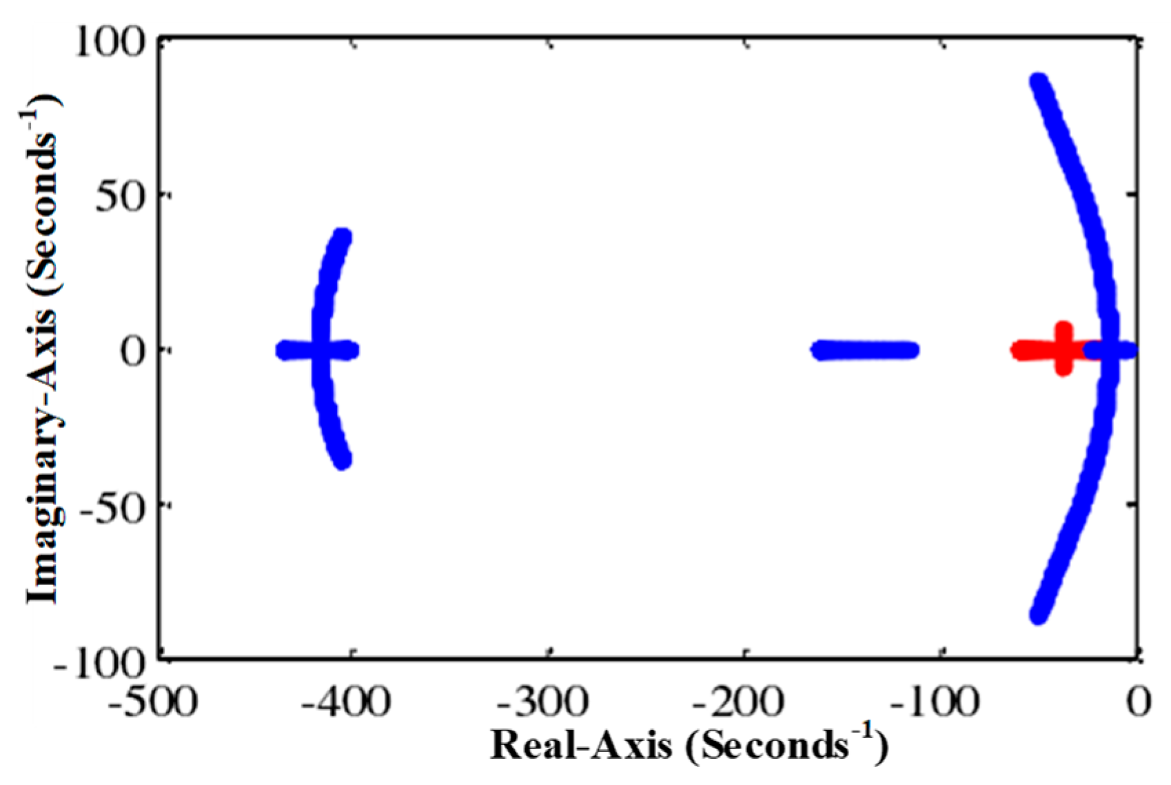
Combined with the simulation parameters of the electrically excited synchronous motor, the pole distribution of the motor below the rated speed designed by the reduced-order observer method can be made and shown in Figure 3:

The blue line is the pole distribution of the motor below the rated speed solved by the determinant equation $\det (sI-P)=0$ under the fifth-order equation of the state, and the red line is the pole distribution of the motor below the rated speed solved by the reduced-order equation $\det [sI-(P_{11}+K{P}_{21})]=0$ under the determinant equation. As can be seen from the figure, the selection of feedback matrix K meets the design requirements, and the stability of the system can still be guaranteed after the reduced-order observer design method is adopted.

3.3. Discretization Algorithm and Related Stability Analysis

5.

First-order forward difference method

Set $du(t)/dt=e(t)$, then, the formula of first-order forward difference method is:

$$\frac{u(k+1)-u(k)}{T}=e(k)$$

(20)

In the first-order forward difference method, the s plane has the following transformation relation with the z plane:

$$s=\frac{z-1}{T}$$

(21)

To obtain the mapping relationship between s plane and z plane, let the poles of the motor in s plane be $s=p+jq$, according to Equation (21):

$$z=1+Ts=(1+pT)+jqT$$

(22)

After discretization, the stability condition of the system is as follows: the poles on the s plane of the motor must be in the unit circle of the z plane when they are mapped to the z plane. The two ends of Equation (22) are squared and ${\left|z\right|}^2<1$ is used to obtain the following relation:

$$\frac{1}{T^2}>{(\frac{1}{T}+p)}^2+q^2$$

(23)

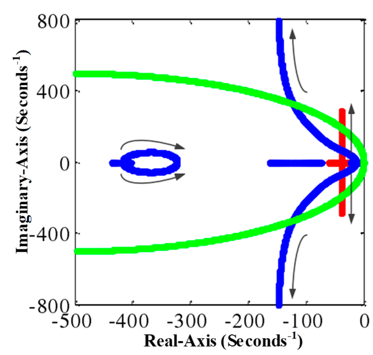
Therefore, only when the motor poles are in a stable circle with (−1/T, 0) as the center of the circle and a radius of 1/T in the s plane can the discretized system be stable. Under the condition that the sampling period T decreases and the motor speed increases in the case of the weak magnetic field, the pole distribution diagram of the EESM before and after order reduction is made, as shown in the figure below. The motor pole distribution in blue was obtained by using the determinant equation $\det (sI-P)=0$ before using the reduced-order observer design method. The motor pole distribution in red was obtained by using the determinant equation $\det [sI-(P_{11}+K{P}_{21})]=0$ after the design method of the reduced-order observer. The green color is the stable circle at low switching frequency with sampling cycle T = 0.002 s (500 Hz).

As can be seen from the figure, in the case of a low sampling period, as the speed increases, the motor pole will be outside the stable circle, and the system at this time also tends to be unstable. Therefore, when the first-order forward difference method is used for discretization, it will be constrained by the sampling frequency and the motor speed.

6.

The bilinear transformation method

Set $du(t)/dt=e(t)$, then, the formula of the bilinear transformation method is:

$$\frac{u(k)-u(k-1)}{T}=\frac{e(k)+e(k-1)}{2}$$

(24)

In the bilinear transformation method, the transformation relation between s plane and z plane is:

$$s=\frac{2}{T}\frac{z-1}{z+1}$$

(25)

Substituting $s=p+jq$ into Equation (25), we can get:

$$z=\frac{1+\frac{T}{2}s}{1-\frac{T}{2}s}=\frac{(1+\frac{T}{2}p)+j\frac{qT}{2}}{(1-\frac{T}{2}p)-j\frac{qT}{2}}$$

(26)

Square the magnitude of both sides:

$${\left|z\right|}^2=\frac{{(1+\frac{T}{2}p)}^2+{(j\frac{qT}{2})}^2}{{(1-\frac{T}{2}p)}^2-{(j\frac{qT}{2})}^2}<1$$

(27)

When a < 0 (left half of the s plane) is satisfied, the s plane is mapped to $\left|z\right|<1$ (inside the unit circle of the z plane). As can be seen from Figure 4, the poles of the motors before and after the design of the reduced-order flux observer are distributed in the left half-plane of the s plane and are mapped in the unit circle when they are in the z plane. Therefore, when adopting the bilinear transformation method for discretization, the sampling period T and the range of speed need not be considered, which can ensure the stability of the motor system after discretization.

3.4. Analysis of the Influence of Motor Parameter Variation on the Motor System Based on the Reduced-Order Flux Observer

Since the state observer depends very much on the motor model, the change of motor parameters has a great influence on the state observer. In the process of motor operation, due to the influence of temperature, magnetic saturation, motor operating frequency and other factors, the motor parameters will produce deviation, which will lead to inaccurate observation results of the state observer.

In this paper, the system stability is analyzed by analyzing the distribution of the poles when the relevant parameters of the motor change by ±50%, and then the simulation analysis of the vector control system of the EESM is carried out by combining with the parameter change conditions.

Through the above analysis, it can be known that the stability of the motor system can be analyzed through the pole distribution diagram of the motor system. Before the design of the reduced-order flux observer with feedback matrix, the motor state equation can be regarded as an open-loop full-order observer. At this time, the motor pole distribution graph can be obtained from the determinant equation det(sI − P) = 0, which is the fifth-order equation. After the design of the reduced-order observer with feedback matrix, the flux observer has the closed-loop characteristic, and the pole distribution of the motor is obtained by the determinant equation det[sI − (P₁₁ + KP₂₁)] = 0, which is the second-order equation. At different speeds, the pole distribution of the motor can be drawn by solving the corresponding determinant equation.

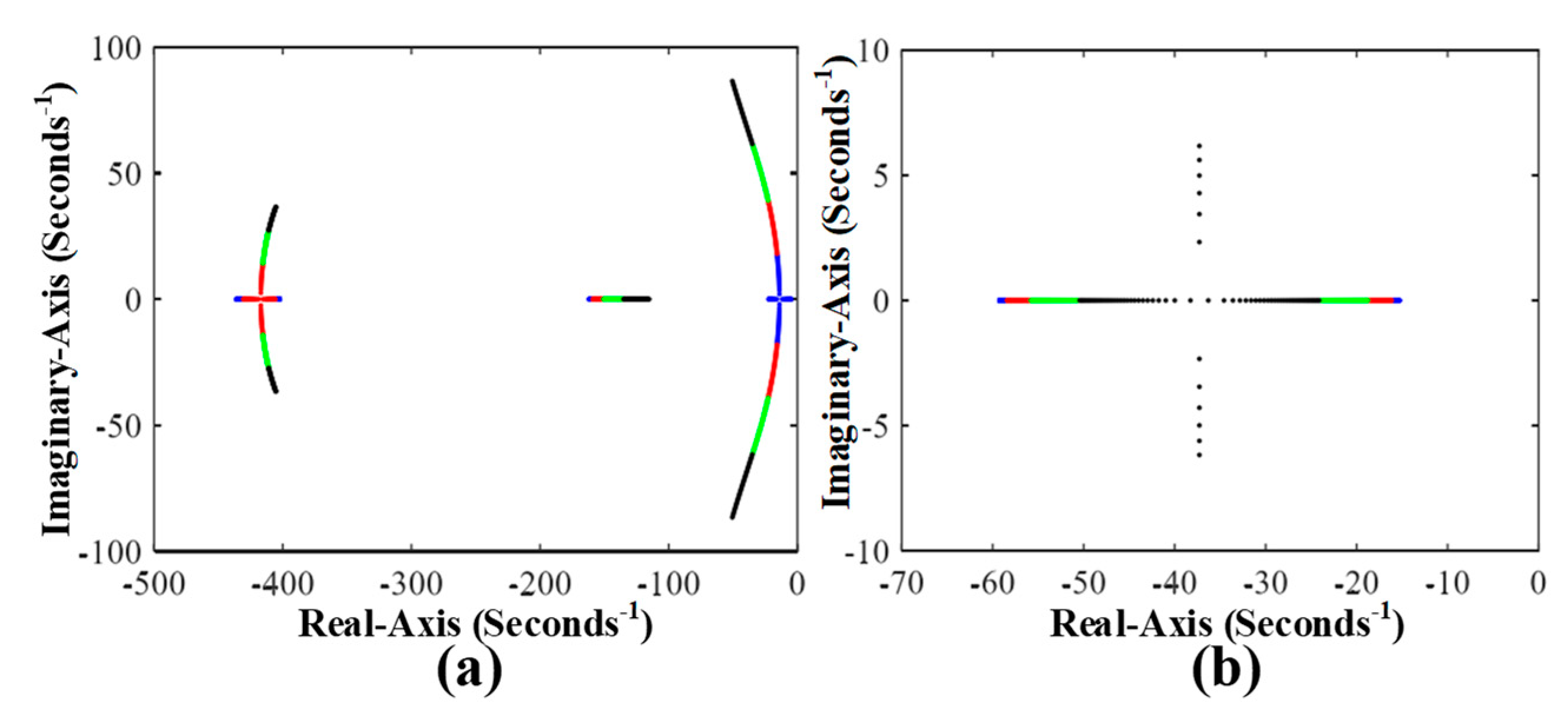
When the rated speed is below, draw the motor pole distribution diagram for different speed segments, as shown in Figure 5.

In Figure 5, the blue segment is the motor pole distribution at the speed of 0–400 rpm, the red segment is the motor pole distribution at the speed of 400–800 rpm, the green segment is the motor pole distribution at the speed of 800–1200 rpm, and the black segment is the motor pole distribution at the speed of 1200–1500 rpm. As can be seen from the figure, before the design of the reduced-order observer was not adopted, the motor state equation was a fifth order equation. Under this condition, the system determinant was a fifth order equation, and the poles of the system expanded outward with the increase of speed. After the reduced-order observer design about the feedback matrix, the motor state equation is of second order, the system determinant is of second order, the poles of the motor first converge and then divergent up and down with the increase of the motor speed.

• Stator resistance to system stability analysis

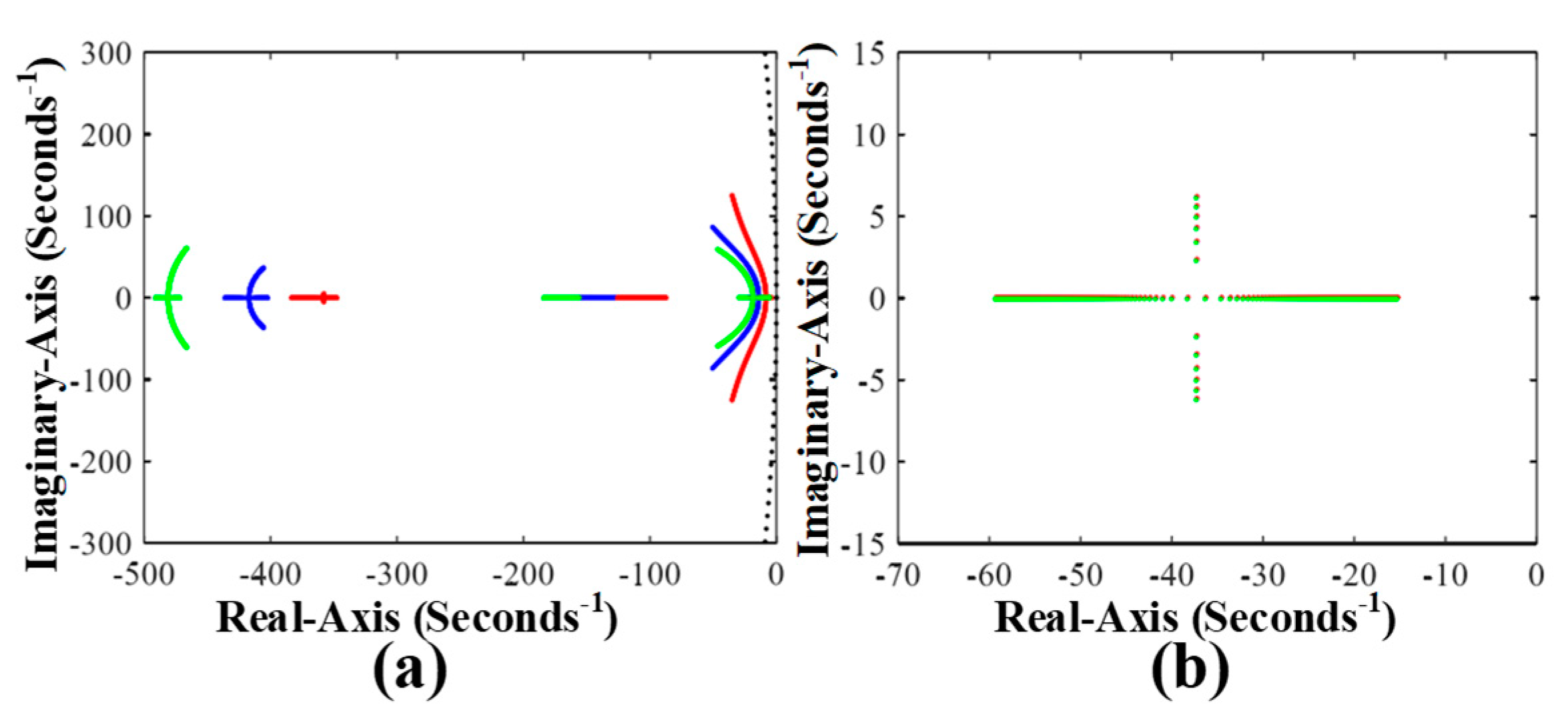
When the stator resistance changes by ±50%, the pole distribution of the EESM before and after the design is shown in Figure 6. In the figure, blue is the motor pole distribution curve when the stator resistance is R_s, green is the motor pole distribution curve when the stator resistance is 1.5 R_s, red is the motor pole distribution curve when the stator resistance is 0.5 R_s, black is the stable circle with the discrete frequency of 5 kHz.

As can be seen from Figure 6a, in the full-order state without a feedback matrix, when the resistance value of stator resistance decreases, the motor pole shifts to the right, close to the virtual axis, and with the increase of speed, the deviation from the normal curve will become larger and larger, and there is an obvious tendency to break away from the stable circle. When the discrete frequency decreases and the stable circle becomes small, the system will be unstable. When the resistance value increases, the motor pole will deviate from the normal curve to the left to a large extent. As can be seen from Figure 6b, in the reduced-order state with the feedback matrix, the stability of the system is not affected by changes in stator resistance parameters.

2.

Rotor resistance to system stability analysis

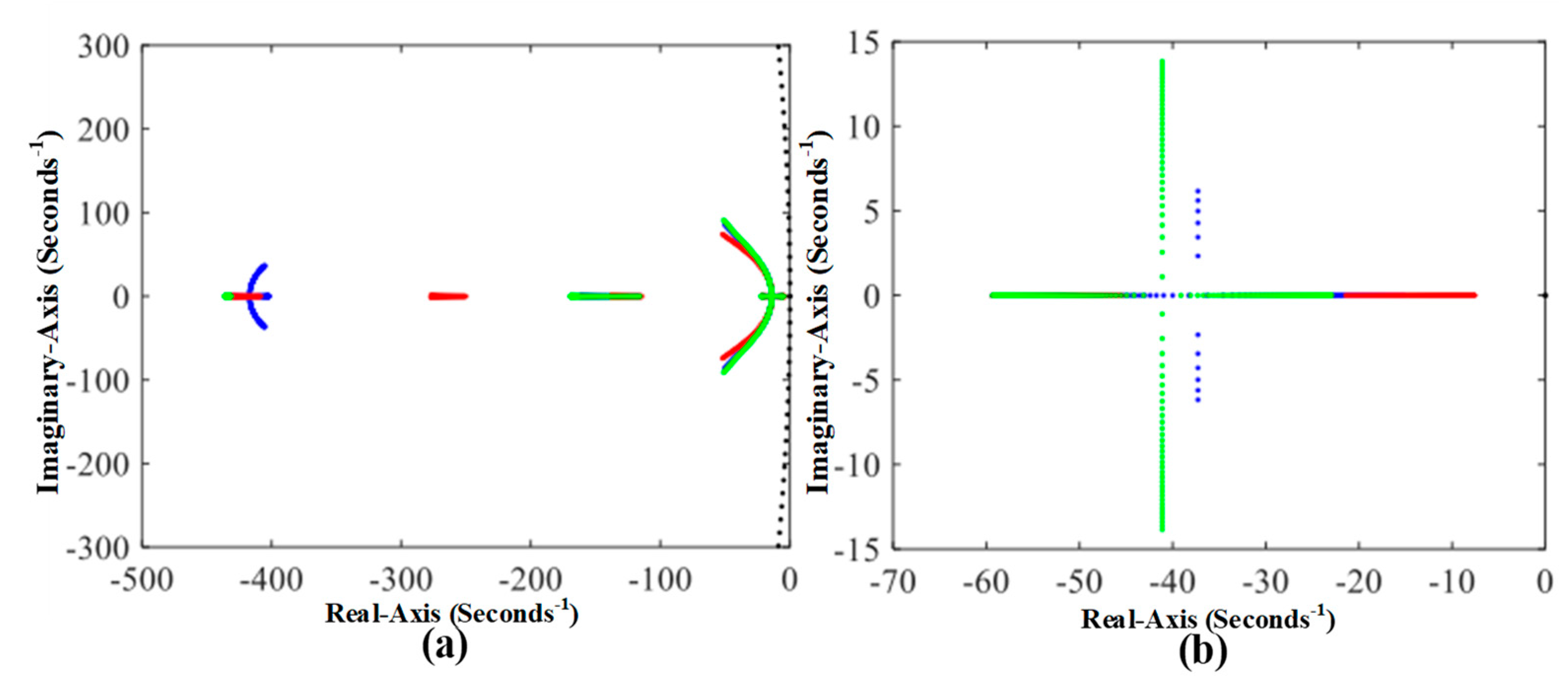
When the rotor resistance changes by ±50%, the pole distribution of the EESM before and after the design is shown in Figure 7.

In Figure 7, blue is the pole distribution curve of the motor with rotor resistance of R_f, green is the pole distribution curve of the motor with rotor resistance of 1.5 R_f, red is the pole distribution curve of the motor with rotor resistance of 0.5 R_f, black is the stable circle with the discrete frequency of 5 kHz. As can be seen from Figure 7a, in the full-order state without a feedback matrix, when the resistance value of the rotor is reduced, the poles of the motor as a whole shift to the left. With the increase of speed, the poles first deviate from the normal curve and then approach the normal curve. Although they are far away from the virtual axis, the poles quickly diverge along the direction of the virtual axis with the increase of speed. When the discrete frequency decreases and the stable circle becomes smaller, instability will occur. When the rotor resistance increases, the pole distribution of the motor will not deviate from the normal curve. It can be seen from Figure 7b that the system stability is not affected by changes in rotor resistance parameters in the reduced-order state of the feedback matrix.

3.

Analysis of damping d axis resistance to system stability

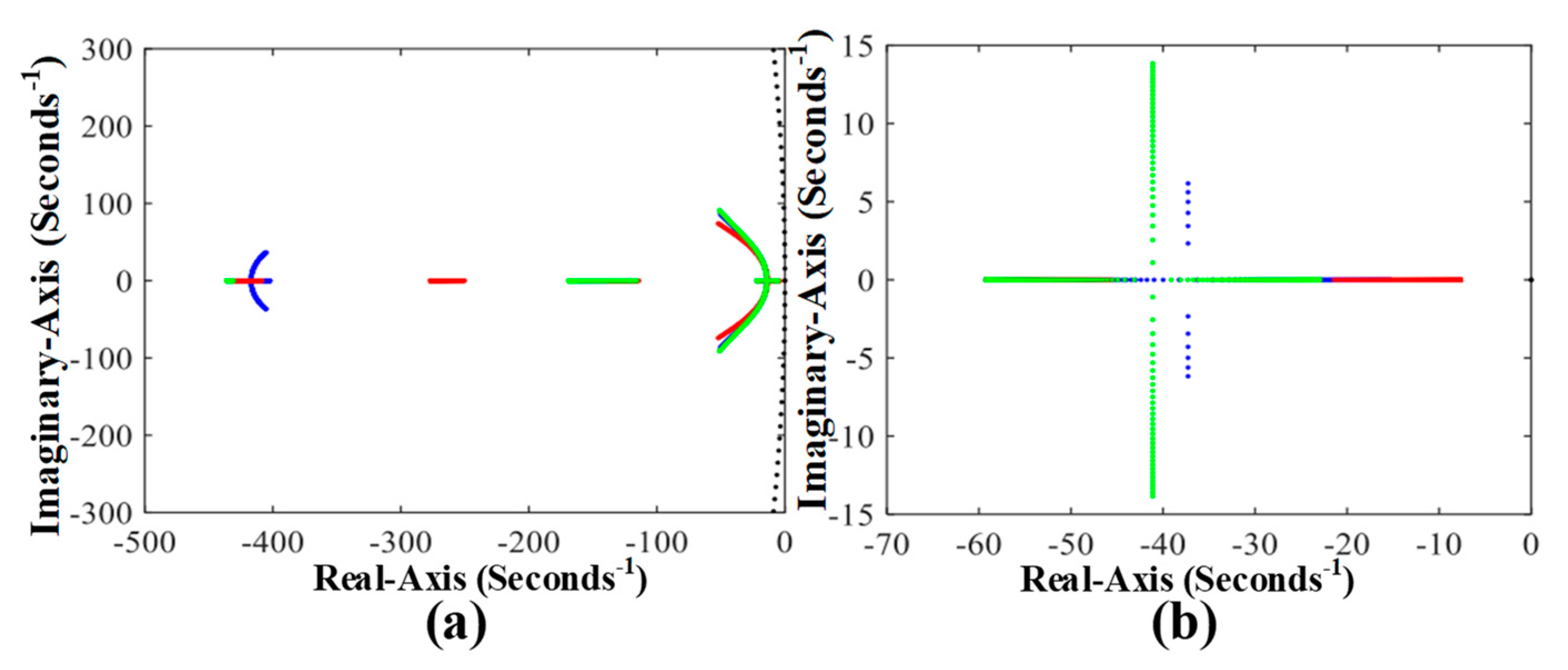
When the resistance of the damping d axis changes by ±50%, the pole distribution of the EESM before and after design is shown in Figure 8.

In Figure 8, blue is the pole distribution curve of the motor with the resistance of the damped d axis R_Dd, green is the pole distribution curve of the motor with the resistance of the damped d axis 1.5 R_Dd, red is the pole distribution curve of the motor with the resistance of the damped d axis 0.5 R_Dd, and black is the stable circle with the discrete frequency of 5 kHz. As can be seen from Figure 8a, in the full-order state without a feedback matrix, the resistance of the damped d axis has little influence on the stability of the system. When the resistance of the damped d axis decreases, it deviates from the normal curve. As can be seen from Figure 8b, in the order reduction state of the feedback matrix, when the resistance value of the damping d axis decreases, it will move to the imaginary axis, and when the resistance value increases, it will move to the left.

4.

Analysis of damping q axis resistance to system stability

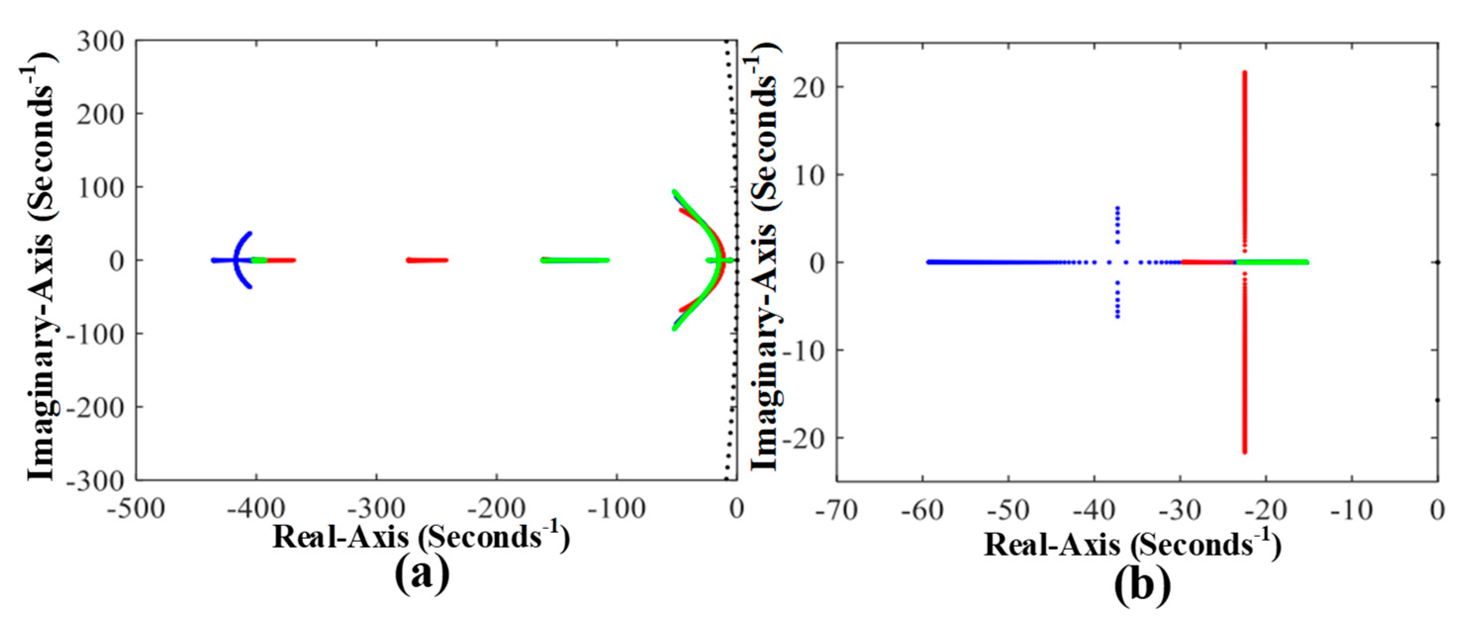
When the resistance of the damping q axis changes by ±50%, the pole distribution of EESM before and after the design is shown in Figure 9.

In Figure 9, blue is the pole distribution curve of the motor with the resistance of the damped q axis as R_Dq, green is the pole distribution curve of the motor with the resistance of the damped q axis as 1.5 R_Dq, red is the pole distribution curve of the motor with the resistance of the damped q axis as 0.5 R_Dq, and black is the stable circle with the discrete frequency of 5 kHz. As can be seen from Figure 9a, in the full-order state without a feedback matrix, the damped q axis resistance has little influence on the stability of the system. When the damped q axis resistance decreases, it will deviate from the normal curve. As can be seen from Figure 9b, in the down-order closed-loop state, when the resistance value of the damping q axis increases or decreases, it will move to the imaginary axis. However, when the resistance value decreases, the poles of the motor will increase rapidly along the imaginary axis as the speed increases. When the discrete frequency decreases and the stable circle becomes small, instability will occur.

5.

Analysis of stability of the system by the inductance of armature d axis

When the inductance of the armature d axis changes by ±50%, the pole distribution of the EESM before and after the design is shown in Figure 10.

In Figure 10, blue is the pole distribution curve of the motor with the inductance of the armature d axis L_ad, green is the pole distribution curve of the motor with the inductance of the armature d axis 1.5 L_ad, red is the pole distribution curve of the motor with the inductance of the armature d axis 0.5 L_ad, and black is the stable circle with the discrete frequency of 5 kHz. It can be seen from Figure 10a that the inductance of the armature d axis has little influence on the stability of the system in the full-order state without a feedback matrix. As can be seen from Figure 10b, in the down-order closed-loop state, when the inductance value of the armature d axis decreases, the motor pole shifts to the left and rapidly diverges along the virtual axis with the increase of the rotational speed. When the discrete frequency decreases and the stable circle becomes small, instability will occur.

6.

Analysis of stability of the system by the inductance of armature q axis

When the inductance of the armature q axis changes by ±50%, the pole distribution of the EESM before and after the design is shown in Figure 11.

In Figure 11, blue is the pole distribution curve of the motor when the armature q axis inductance L_aq, green is the pole distribution curve when the armature q axis inductance 1.5 L_aq, red is the pole distribution curve when the armature q axis inductance 0.5 L_aq, black is the stable circle with the discrete frequency of 5 kHz. As can be seen from Figure 11a, in the full-order state without a feedback matrix, when the inductance value of the armature q axis decreases, the motor pole will shift from the normal curve. When the inductance value of the armature q axis increases, the influence will be small. As can be seen from Figure 11b, in the down-order closed-loop state, no matter the inductance value of the armature q axis increases or decreases, the pole of the motor shifts to the right. When the inductance value of the armature q axis increases, it quickly diverges along the direction of the virtual axis with the increase of the rotational speed.

4. Simulated Analysis

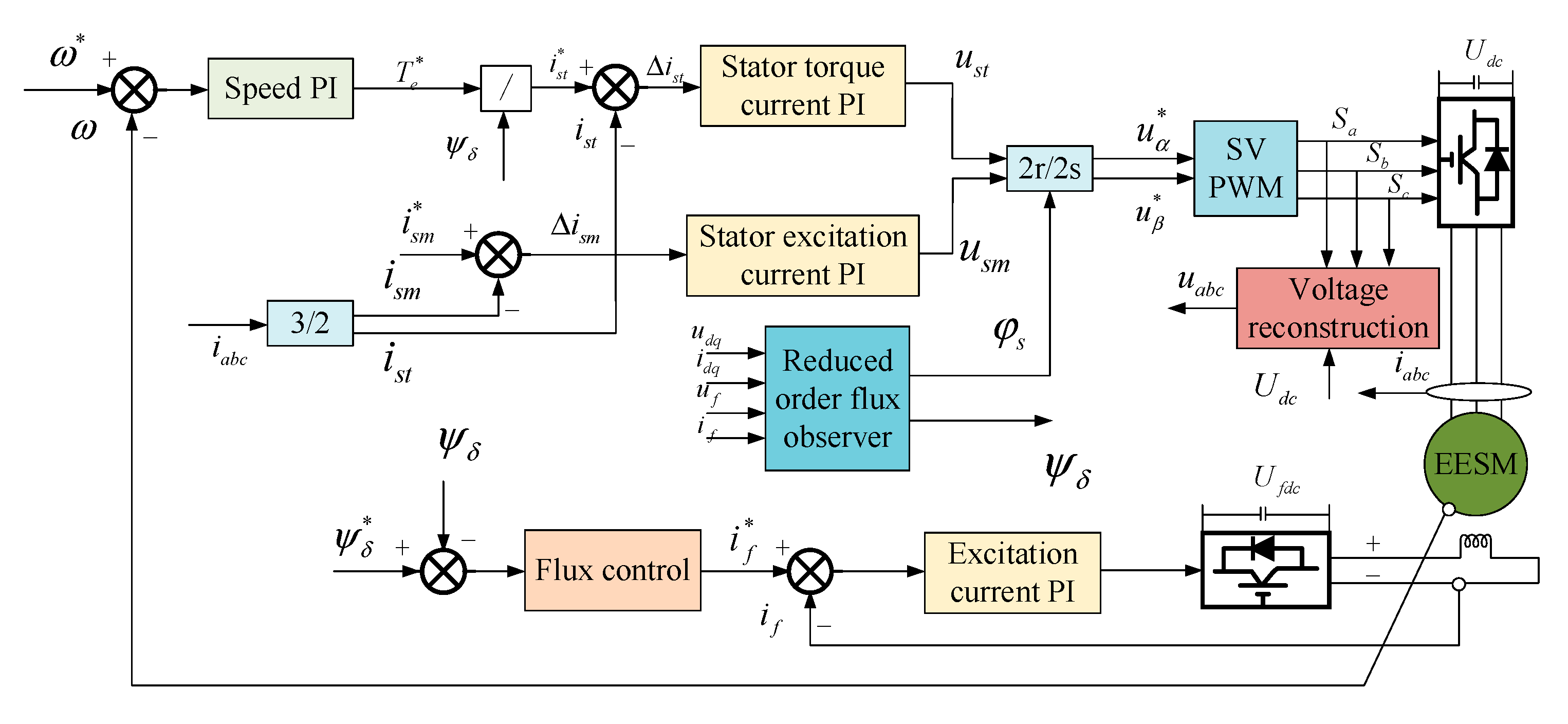
MATLAB/Simulink was used to simulate the reduced-order flux observer discrete by the two discretization methods, and the motor parameters were shown in

Table 3. EESM parameters.

Specification	Value	Specification	Value
Power (kW)	8	q axis armature reaction inductance (mH)	51.8
DC-link voltage (V)	380	Stator winding leakage inductance (mH)	4.5
Rated speed (r/min)	1500	Rotor winding leakage inductance (mH)	11.3
Number of pole pairs	2	d axis damping winding resistance (Ω)	3.14
Stator resistance (Ω)	1.62	q axis damping winding resistance (Ω)	4.77
Rotor resistance (Ω)	1.2	d axis damping winding leakage inductance (mH)	7.33
d axis armature reaction inductance (mH)	108.6	q axis damping winding leakage inductance (mH)	10.15

. Figure 12 is the block diagram of the vector control system of an EESM with air gap flux orientation.

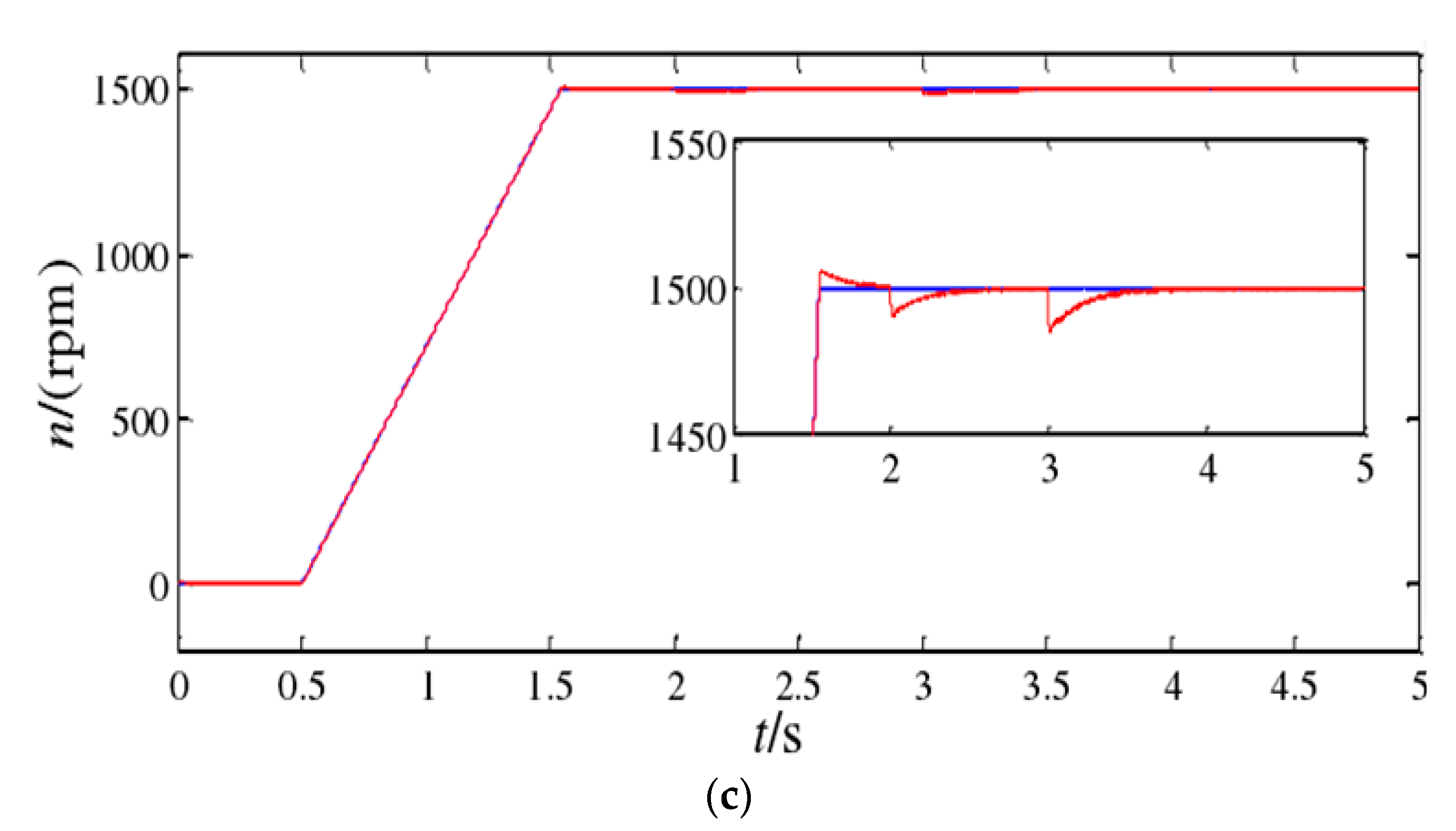
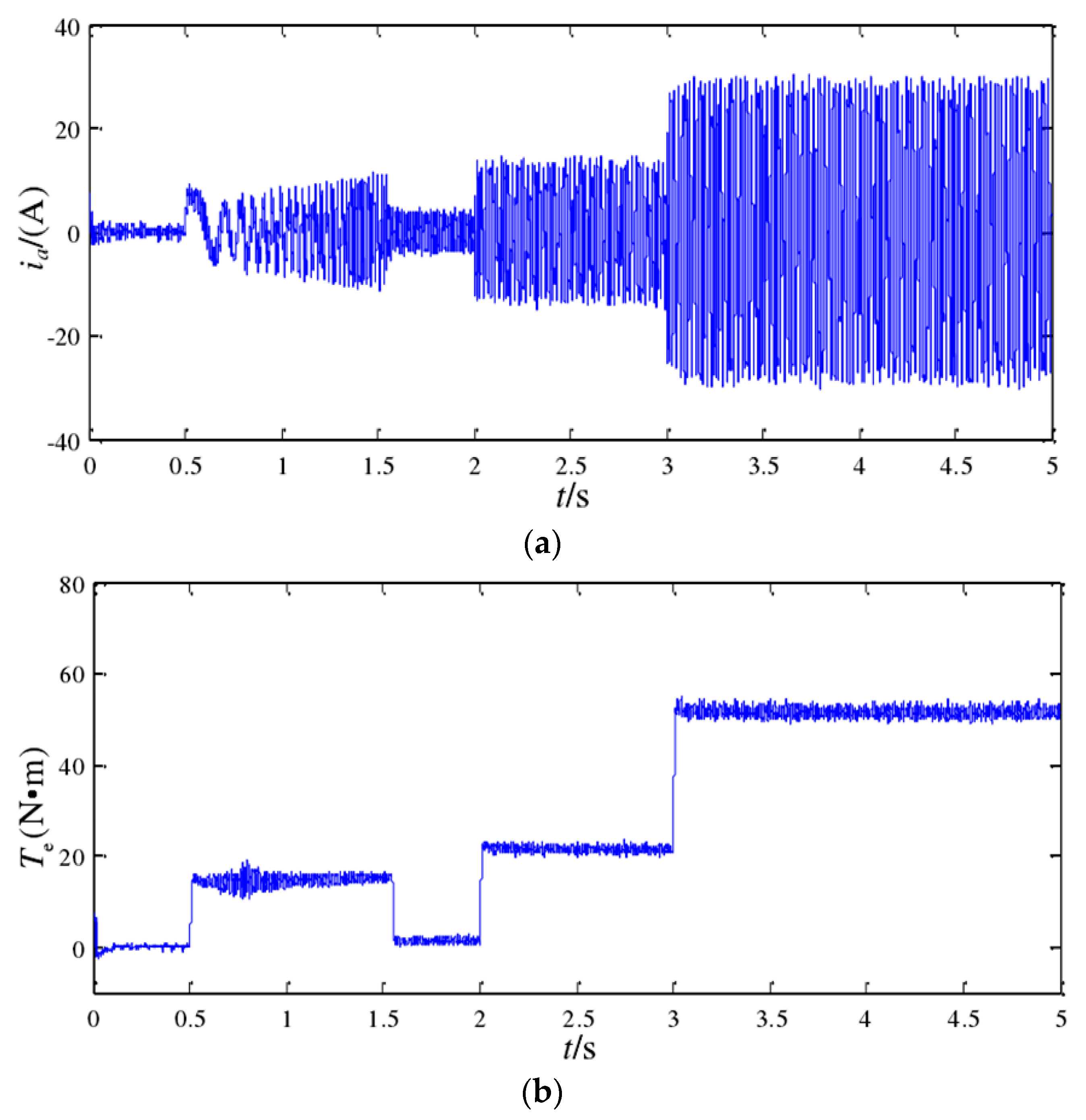
The simulation waveform of the discrete observer using the first-order forward difference method is shown in Figure 13. Figure 13a shows the stator current waveform, Figure 13b the torque waveform and Figure 13c the speed waveform. In the simulation, the rated speed of the motor is 1500 rpm, 20 Nm load is added at 2 s, and 51 Nm load is added at 3 s. The stator current harmonic is little when the torque changes and the motor speed can reach the rated speed, and when the load torque changes, there is no big fluctuation.

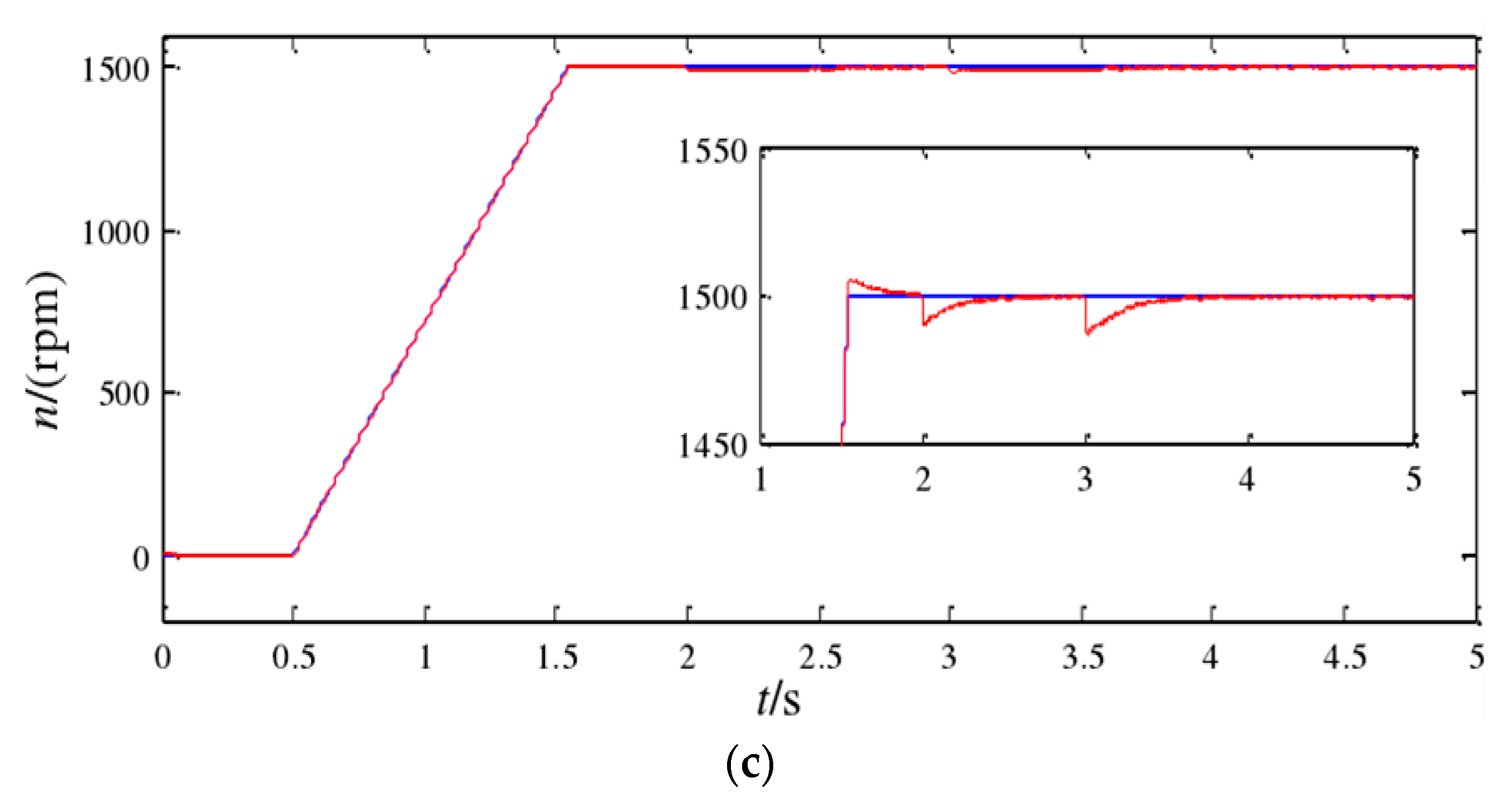
The simulation waveform of the discrete observer using the bilinear transformation method is shown in Figure 14. The condition is the same as the simulation waveform of the discrete observer using the first-order forward difference method. Compared to Figure 13, the amplitude of stator current using the bilinear transformation method is smaller than that using the first-order forward difference method. The load waveform also has few fluctuations compared to that in Figure 13.

In the simulation, the sampling period is T = 0.0002 s (5 kHz), and the maximum speed is the rated speed of 1500 rpm. It can be seen from the simulation waveform that the reduced-order flux observer, using the two discretization methods, has achieved all the control objectives in the simulation, and the speed has a small drop during loading, but it all returns to the given value after a short period of adjustment, ensuring the stable operation of the system.

5. Conclusions

In the speed control system of electrically excited synchronous motor (EESM), the flux observer plays an important role, which can detect the rotating angle and the amplitude of flux. In this paper, a reduced-order flux observer is designed by combining the state observer of modern control theory and the state equation of EESM. The first-order forward difference method and the bilinear transform method are used to discretize the reduced-order flux observer and the stability of the motor system after discretization is analyzed.

While motor operations, motor parameters will change with temperature magnetic saturation, motor operating frequency and other factors. This paper studies the influence of parameter changes on the motor system by using the change of the pole distribution of the motor system. It is worth noting that according to the distribution diagram of motor poles, when the constant rotor resistance changes, the stability of the system is not affected by parameter changes after adopting the reduced-order feedback matrix. When the inductance of the dq axis of the motor changes, the feedback matrix has little influence on the stability of the system.

Finally, it can be seen from the simulation that the reduced-order flux observer can accurately estimate the motor flux and flux angle, and the motor can run stably in the vector control system of the electrically excited synchronous motor using the reduced-order flux observer.

In the future, other flux observer methods will be studied, such as the first order forward difference method and the bilinear transformation method. Different from other synchronous motor, EESM has a complex mathematic model and high coupling characteristics, thus high performance and stability flux observers need to be paid attention to.

References

- Sun, X.; Jin, Z.; Wang, S.; Yang, Z.; Li, K.; Fan, Y.; Chen, L. Performance Improvement of Torque and Suspension Force for a Novel Five-Phase BFSPM Machine for Flywheel Energy Storage Systems. IEEE Trans. Appl. Supercond. 2019, 29, 1–5. [Google Scholar] [CrossRef]
- Su, J.; Gao, R.; Husain, I. Model Predictive Control Based Field-Weakening Strategy for Traction EV Used Induction Motor. IEEE Trans. Ind. Appl. 2017, 54, 2295–2305. [Google Scholar] [CrossRef]
- Sun, X.; Hu, C.; Lei, G.; Yang, Z.; Guo, Y.; Zhu, J. Speed sensorless control of SPMSM drives for EVs with a binary search algo-rithm-based phase-locked loop. IEEE Trans. Veh. Technol. 2020, 69, 4968–4978. [Google Scholar] [CrossRef]
- Sun, X.; Cao, J.; Lei, G.; Guo, Y.; Zhu, J. A Robust Deadbeat Predictive Controller with Delay Compensation Based on Composite Sliding-Mode Observer for PMSMs. IEEE Trans. Power Electron. 2021, 36, 10742–10752. [Google Scholar] [CrossRef]
- Ding, H.; Zhu, H.; Hua, Y. Optimization Design of Bearingless Synchronous Reluctance Motor. IEEE Trans. Appl. Supercond. 2018, 28, 1–5. [Google Scholar] [CrossRef]
- Chen, L.; Xu, H.; Sun, X.; Cai, Y. Three-Vector-Based Model Predictive Torque Control for a Permanent Magnet Synchronous Motor of EVs. IEEE Trans. Transp. Electrif. 2021, 7, 1454–1465. [Google Scholar] [CrossRef]
- Shi, Z.; Sun, X.; Cai, Y.; Yang, Z.; Lei, G.; Guo, Y.; Zhu, J. Torque Analysis and Dynamic Performance Improvement of a PMSM for EVs by Skew Angle Optimization. IEEE Trans. Appl. Supercond. 2019, 29, 1–5. [Google Scholar] [CrossRef]
- Kali, Y.; Ayala, M.; Rodas, J.; Saad, M.; Doval-Gandoy, J.; Gregor, R.; Benjelloun, K. Current Control of a Six-Phase Induction Machine Drive Based on Discrete-Time Sliding Mode with Time Delay Estimation. Energies 2019, 12, 170. [Google Scholar] [CrossRef] [Green Version]
- Gong, C.; Hu, Y.; Gao, J.; Wang, Y.; Yan, L. An Improved Delay-Suppressed Sliding-Mode Observer for Sensorless Vector-Controlled PMSM. IEEE Trans. Ind. Electron. 2020, 67, 5913–5923. [Google Scholar] [CrossRef]
- Sun, X.; Su, B.; Wang, S.; Yang, Z.; Lei, G.; Zhu, J.; Guo, Y. Performance Analysis of Suspension Force and Torque in an IBPMSM with V-Shaped PMs for Flywheel Batteries. IEEE Trans. Magn. 2018, 54, 1–4. [Google Scholar] [CrossRef]
- Hu, W.; Ruan, C.; Nian, H.; Sun, D. Simplified Modulation Scheme for Open-End Winding PMSM System with Common DC Bus Under Open-Phase Fault Based on Circulating Current Suppression. IEEE Trans. Power Electron. 2019, 35, 10–14. [Google Scholar] [CrossRef]
- Sun, Y.; Su, B.; Sun, X. Optimal Design and Performance Analysis for Interior Composite-Rotor Bearingless Permanent Magnet Synchronous Motors. IEEE Access 2018, 7, 7456–7465. [Google Scholar] [CrossRef]
- Yang, Z.; Ji, J.; Sun, X.; Zhu, H.; Zhao, Q. Active Disturbance Rejection Control for Bearingless Induction Motor Based on Hyperbolic Tangent Tracking Differentiator. IEEE J. Emerg. Sel. Top. Power Electron. 2019, 8, 2623–2633. [Google Scholar] [CrossRef]
- Nuutinen, P.; Pinomaa, A.; Peltoniemi, P.; Kaipia, T.; Karppanen, J.; Silventoinen, P. Common-Mode and RF EMI in a Low-Voltage DC Distribution Network with a PWM Grid-Tie Rectifying Converter. IEEE Trans. Smart Grid 2016, 8, 400–408. [Google Scholar] [CrossRef]
- Yang, Z.; Ding, Q.; Sun, X.; Zhu, H.; Lu, C. Fractional-order sliding mode control for a bearingless induction motor based on improved load torque observer. J. Frankl. Inst. 2021, 358, 3701–3725. [Google Scholar] [CrossRef]
- Karttunen, J.; Kallio, S.; Honkanen, J.; Peltoniemi, P.; Silventoinen, P. Partial Current Harmonic Compensation in Dual Three-Phase PMSMs Considering the Limited Available Voltage. IEEE Trans. Ind. Electron. 2017, 64, 1038–1048. [Google Scholar] [CrossRef]
- Sun, X.; Hu, C.; Lei, G.; Guo, Y.; Zhu, J. State feedback control for a PM hub motor based on grey wolf optimization algorithm. IEEE Trans. Power Electron. 2020, 35, 1136–1146. [Google Scholar] [CrossRef]
- Gu, L.; Peng, K. A Single-Stage Fault-Tolerant Three-Phase Bidirectional AC/DC Converter with Symmetric High-Frequency Y-Δ Connected Transformers. IEEE Trans. Power Electron. 2020, 35, 9226–9237. [Google Scholar] [CrossRef]
- Sun, X.; Shi, Z.; Cai, Y.; Lei, G.; Guo, Y.; Zhu, J. Driving-Cycle-Oriented Design Optimization of a Permanent Magnet Hub Motor Drive System for a Four-Wheel-Drive Electric Vehicle. IEEE Trans. Transp. Electrif. 2020, 6, 1115–1125. [Google Scholar] [CrossRef]
- Sun, X.; Shi, Z.; Lei, G.; Guo, Y.; Zhu, J. Analysis and Design Optimization of a Permanent Magnet Synchronous Motor for a Campus Patrol Electric Vehicle. IEEE Trans. Veh. Technol. 2019, 68, 10535–10544. [Google Scholar] [CrossRef]
- Jin, Z.; Sun, X.; Lei, G.; Guo, Y.; Zhu, J. Sliding Mode Direct Torque Control of SPMSMs Based on a Hybrid Wolf Optimization Algorithm. IEEE Trans. Ind. Electron. 2021, online. [Google Scholar] [CrossRef]
- Han, J.; Kum, D.; Park, Y. Synthesis of Predictive Equivalent Consumption Minimization Strategy for Hybrid Electric Vehicles Based on Closed-Form Solution of Optimal Equivalence Factor. IEEE Trans. Veh. Technol. 2017, 66, 5604–5616. [Google Scholar] [CrossRef]
- Shi, Z.; Sun, X.; Cai, Y.; Tian, X.; Chen, L. Design optimization of an outer-rotor permanent magnet synchronous hub motor for a low-speed campus patrol EV. IET Electr. Power Appl. 2020, 14, 2111–2118. [Google Scholar] [CrossRef]
- Reddy, C.U.; Prabhakar, K.K.; Singh, A.K.; Kumar, P. Speed Estimation Technique Using Modified Stator Current Error-Based MRAS for Direct Torque Controlled Induction Motor Drives. IEEE J. Emerg. Sel. Top. Power Electron. 2019, 8, 1223–1235. [Google Scholar] [CrossRef]
- Li, K.; Ling, F.; Sun, X.; Zhao, D.; Yang, Z. Reactive-power-based MRAC for rotor resistance and speed estimation in bearingless induction motor drives. Int. J. Appl. Electromagn. Mech. 2020, 62, 127–143. [Google Scholar] [CrossRef]
- Sun, X.; Zhang, Y.; Tian, X.; Cao, J.; Zhu, J. Speed Sensorless Control for IPMSMs Using a Modified MRAS with Grey Wolf Optimization Algorithm. IEEE Trans. Transp. Electrif. 2021. [Google Scholar] [CrossRef]
- Pupadubsin, R.; Chayopitak, N.; Taylor, D.G.; Nulek, N.; Kachapornkul, S.; Jitkreeyarn, P.; Somsiri, P.; Tungpimolrut, K. Adaptive Integral Sliding-Mode Position Control of a Coupled-Phase Linear Variable Reluctance Motor for High-Precision Applications. IEEE Trans. Ind. Appl. 2012, 48, 1353–1363. [Google Scholar] [CrossRef]
- Foo, G.; Rahman, M.F. Sensorless Sliding-Mode MTPA Control of an IPM Synchronous Motor Drive Using a Sliding-Mode Observer and HF Signal Injection. IEEE Trans. Ind. Electron. 2010, 57, 1270–1278. [Google Scholar] [CrossRef]
- Sun, X.; Cao, J.; Lei, G.; Guo, Y.; Zhu, J. A Composite Sliding Mode Control for SPMSM Drives Based on a New Hybrid Reaching Law with Disturbance Compensation. IEEE Trans. Transp. Electrif. 2021, 7, 1427–1436. [Google Scholar] [CrossRef]
- Shahnazi, R.; Shanechi, H.; Pariz, N. Position Control of Induction and DC Servomotors: A Novel Adaptive Fuzzy PI Sliding Mode Control. IEEE Trans. Energy Convers. 2008, 23, 138–147. [Google Scholar] [CrossRef]
- Sun, X.; Feng, L.; Diao, K.; Yang, Z. An Improved Direct Instantaneous Torque Control Based on Adaptive Terminal Sliding Mode for a Segmented-Rotor SRM. IEEE Trans. Ind. Electron. 2021, 68, 10569–10579. [Google Scholar] [CrossRef]
- Junejo, A.K.; Xu, W.; Mu, C.; Ismail, M.M.; Liu, Y. Adaptive Speed Control of PMSM Drive System Based a New Sliding-Mode Reaching Law. IEEE Trans. Power Electron. 2020, 35, 12110–12121. [Google Scholar] [CrossRef]
- Che, H.S.; Duran, M.J.; Levi, E.; Jones, M.; Hew, W.P.; Rahim, N.A. Post-fault operation of an asymmetrical six-phase induction machine with single and two isolated neutral points. IEEE Energy Convers. Congr. Expo. 2013, 29, 1131–1138. [Google Scholar]
- Sun, X.; Wu, J.; Lei, G.; Guo, Y.; Zhu, J. Torque Ripple Reduction of SRM Drive Using Improved Direct Torque Control With Sliding Mode Controller and Observer. IEEE Trans. Ind. Electron. 2021, 68, 9334–9345. [Google Scholar] [CrossRef]
- Bermúdez, M.; Gonzalez-Prieto, I.; Barrero, F.; Guzman, H.; Duran, M.J.; Kestelyn, X. Open-Phase Fault-Tolerant Direct Torque Control Technique for Five-Phase Induction Motor Drives. IEEE Trans. Ind. Electron. 2016, 64, 902–911. [Google Scholar] [CrossRef] [Green Version]
- Wang, X.; Wang, Z.; Xu, Z.; Cheng, M.; Hu, Y. Optimization of Torque Tracking Performance for Direct-Torque-Controlled PMSM Drives with Composite Torque Regu-lator. IEEE Trans. Ind. Electron. 2020, 67, 10095–10108. [Google Scholar] [CrossRef]
- Hernandez, O.S.; Cervantes-Rojas, J.; Oliver, J.O.; Castillo, C.C. Stator Fixed Deadbeat Predictive Torque and Flux Control of a PMSM Drive with Modulated Duty Cycle. Energies 2021, 14, 2769. [Google Scholar] [CrossRef]
- Sun, X.; Diao, K.; Lei, G.; Guo, Y.; Zhu, J. Study on Segmented-Rotor Switched Reluctance Motors with Different Rotor Pole Numbers for BSG System of Hybrid Electric Vehicles. IEEE Trans. Veh. Technol. 2019, 68, 5537–5547. [Google Scholar] [CrossRef]
- Mlot, A.; González, J. Performance Assessment of Axial-Flux Permanent Magnet Motors from a Manual Manufacturing Process. Energies 2020, 13, 2122. [Google Scholar] [CrossRef]
- Grasso, E.; Palmieri, M.; Mandriota, R.; Cupertino, F.; Nienhaus, M.; Kleen, S. Analysis and Application of the Direct Flux Control Sensorless Technique to Low-Power PMSMs. Energies 2020, 13, 1453. [Google Scholar] [CrossRef] [Green Version]
- Karttunen, J.; Kallio, S.; Peltoniemi, P.; Silventoinen, P. Current Harmonic Compensation in Dual Three-Phase PMSMs Using a Disturbance Observer. IEEE Trans. Ind. Electron. 2016, 63, 583–594. [Google Scholar] [CrossRef]
- Chen, L.; Xu, H.; Sun, X. A novel strategy of control performance improvement for six-phase permanent magnet synchronous hub motor drives of EVs under new European driving cycle. IEEE Trans. Veh. Technol. 2021, 70, 5628–5637. [Google Scholar] [CrossRef]
- Li, K.; Cheng, G.; Sun, X.; Yang, Z. A Nonlinear Flux Linkage Model for Bearingless Induction Motor Based on GWO-LSSVM. IEEE Access 2019, 7, 36558–36567. [Google Scholar] [CrossRef]
- Lin, X.; Huang, W.; Jiang, W.; Zhao, Y.; Zhu, S. A Stator Flux Observer with Phase Self-Tuning for Direct Torque Control of Permanent Magnet Synchronous Motor. IEEE Trans. Power Electron. 2019, 35, 6140–6152. [Google Scholar] [CrossRef]
- Xu, W.; Dian, R.; Liu, Y.; Hu, D.; Zhu, J. Robust Flux Estimation Method for Linear Induction Motors Based on Improved Extended State Observers. IEEE Trans. Power Electron. 2019, 34, 4628–4640. [Google Scholar] [CrossRef]
Figure 1.
Reference coordinates of the synchronous motor.
Figure 2.
The structure diagram of the reduced-order flux observer for EESM.
Figure 3.
Pole distribution of motor under rated speed after designed.
Figure 4.
Relationship between pole distribution and stable circle.
Figure 5.
Pole distribution of different speeds under rated speed: (a) pole distribution diagram of motor before design; (b) pole distribution diagram of motor after design.
Figure 6.
Pole distributions of system between different stator resistance: (a) pole distribution diagram of motor before design; (b) pole distribution diagram of motor after design.
Figure 7.
Pole distributions of system between different rotor resistance: (a) pole distribution diagram of motor before design; (b) pole distribution diagram of motor after design.
Figure 8.
Pole distributions of system between different damping resistance in d-axis: (a) pole distribution diagram of motor before design; (b) pole distribution diagram of motor after design.
Figure 9.
Pole distributions of system between different damping resistance in q-axis: (a) pole distribution diagram of motor before design; (b) pole distribution diagram of motor after design.
Figure 10.
Pole distributions of system between different armature inductance in d-axis: (a) pole distribution diagram of motor before design; (b) pole distribution diagram of motor after design.
Figure 11.
Pole distributions of system between different armature inductance in q-axis: (a) pole distribution diagram of motor before design; (b) pole distribution diagram of motor after design.
Figure 12.
Diagram of air gap flux-oriented vector control system for EESM.
Figure 13.
Simulation waveform of EESM by Forward Euler method: (a) a phase stator current waveform; (b) motor torque waveform; (c) motor speed waveform.
Figure 14.
Simulation waveform of bilinear transformation method: (a) a phase stator current waveform; (b) motor torque waveform; (c) motor speed waveform.