
Investigation of Water Injection Influence on Cloud Cavitating Vortical Flow for a NACA66 (MOD) Hydrofoil


School of Energy and Power Engineering, Dalian University of Technology, Dalian 116024, China
*
Author to whom correspondence should be addressed.
Energies 2021, 14(18), 5973; https://doi.org/10.3390/en14185973
Submission received: 31 August 2021
/
Revised: 13 September 2021
/
Accepted: 14 September 2021
/
Published: 20 September 2021
(This article belongs to the Special Issue Advances in Pumped Storage Hydraulic System)
Abstract
:Re-entrant jet causes cloud cavitation shedding, and cavitating vortical flow results in flow field instability. In the present work, a method of water injection is proposed to hinder re-entrant jet and suppress vortex in cloud cavitating flow of a NACA66 (MOD) hydrofoil (Re = 5.1 × 10⁵, σ = 0.83). A combination of filter-based density corrected turbulence model (FBDCM) with the Zwart–Gerber–Belamri cavitation model (ZGB) is adopted to obtain the transient flow characteristics while vortex structures are identified by Q criterion & λ2 criterion. Results demonstrate that the injected water flow reduces the range of the low-pressure zone below 1940 Pa on the suction surface by 54.76%. Vortex structures are observed both inside the attached and shedding cavitation, and the water injection shrinks the vortex region. The water injection successfully blocks the re-entrant jet by generating a favorable pressure gradient (FPG) and effectively weakens the re-entrant jet intensity by 46.98%. The water injection shrinks the vortex distribution area near the hydrofoil suction surface, which makes the flow in the boundary layer more stable. From an energy transfer perspective, the water injection supplies energy to the near-wall flow, and hence keeps the steadiness of the flow field.
1. Introduction
Cavitation widely exists in the low-pressure area of hydraulic machinery [1,2,3]. The collapse of cavitation causes an impact on the blades of hydraulic machines such as hydro turbines, pumps, and propellers [4,5]. Cavitation is often accompanied by noise and severe vibration, resulting in fatigue damage of pumps [6]. Moreover, cavitation has a negative effect on the operation stability and energy performance of hydro turbines in tidal energy conversion [7]. The hydrofoil is a key work component of rotating machinery such as pumps and turbines [8], and the study of its cavitating flow is of great significance; therefore, revealing the mechanism of the cavitation suppression of hydrofoil is helpful to find more efficient and targeted suppression methods.
Cavitation can be manipulated by either active flow control methods or passive methods. The difference between the two strategies is whether additional energy is added [9]. For the passive method, the wall properties of hydrofoil are usually modified in order to control cavitating flow. Che et al. [10] placed an obstacle on the trailing edge of a NACA0015 hydrofoil. They found that it can block re-entrant jet and suppress sheet cavity, but the effect on cavitation control is weak when it comes to the transitional cavity oscillation condition. Zhang et al. [11] arranged obstacles on the hydrofoil to improve the low—pressure distribution in the near-wall region in the cavitating flow field, as a result of weakening the cloud cavitation shedding. Capurso et al. [12] designed slots and guided the fluid from the pressure to suction sides of the hydrofoil to prevent cavitation from developing. Kadivar et al. [13,14] applied cylindrical cavitating-bubble generators (CCGs) on the hydrofoil suction side and found that CCGs can effectively suppress cavitation and reduce the cavitation-induced vibration. Some scholars [15,16] proposed micro vortex generators (VGs) on the hydrofoil leading edge, and they found that vortexes generated from VGs can manipulate the boundary layers. Liu et al. applied a C groove [17,18] and T-shape structures [8] on the hydrofoil tip clearance and successfully suppressed the tip leakage vortex and cavitation inception and development. There are many advantages to the passive control method, such as requiring no external energy and implementing easily; however, the working conditions of hydraulic machinery do not always stay the same in practice [19]; therefore, it is difficult for passive methods to achieve precise adjustment when the working condition of hydraulic machinery changes [20].
The active control methods are different from passive control methods, which usually inject water or gas to the flow field, aiming at improving flow performance or suppressing sheet/cloud cavitation. Maltsev et al. [21] found that when the active method is adopted, the flow separation of hydrofoil with high attack angles is effectively avoided. de Giorgi et al. [22] applied one single synthetic jet-actuator on hydrofoil NACA0015, and they achieved a certain control of the cloud cavitation. Timoshevskiy et al. [9,23,24,25] achieved suppression of sheet cavitation experimentally [26] and numerically by means of the tangential liquid injection to the main flow field. Lu et al. [27] experimentally realized the suppression of cloud cavitation by the active injection method. Wang et al. [28] experimentally studied the influence of active jet flow on sheet/cloud cavitation and reduced the maximum sheet cavity length by 79.4%. Lee et al. [29] even applied the water injection method to a marine propeller and realized the suppression of tip vortex cavitation. The aforementioned active methods can not only improve the flow field, but also can flexibly achieve relatively precise adjustment when working condition changes [19].
The turbulence model plays a vital role in numerical simulation, and the interaction between turbulence and cavitation is very complex [30]. Some empirical coefficients in the numerical model seriously affect the accuracy and uncertainty [31]. Huang et al. blended FBM (filter-based model) [32] with DCM (density correction model) [33] through a function, and they used this new turbulence model to numerically investigate cavitation flow around a Clark-Y hydrofoil. They proved that the new FBDCM model combines the merits of both FBM and DCM, which can capture the details of turbulence flow and the evolution of cavity patterns [34]. Yu et al. [35] verified that the FBDCM model could accurately describe the unsteady cavity shedding on NACA66 hydrofoil. Cheng et al. [36] and Long et al. [37] used the combination of the FBDCM turbulence model and ZGB cavitation model [38] to study the characteristics of cavitation flow around the Clark-Y hydrofoil, showing that this configuration has good prediction accuracy. Based on the FBDCM model, the inception and development of the attached and cloud cavity, and also the characteristics of the multi-scale effect of turbulent flow and multi-phase flow in the cavitation process can be predicted accurately.
At present, explanations for the evolution of sheet cavitation to cloud cavitation are mainly divided into two types: the re-entrant jet mechanism and the shock wave mechanism. Many scholars researched the unsteady characteristic of cavitating flow around hydrofoil caused by re-entrant jet. Kawanami et al. [39] confirmed the existence of the re-entrant jet in the flow field and its remarkable influence on cavity shedding experimentally. Callenaere et al. [40] considered that the re-entrant jet is the main reason for the instability of the flow field, and the re-entrant jet thickness should be given sufficient attention. Ji et al. [41] studied the shedding characteristics of the cavity, and they found that the primary shedding is induced by the collision between the attached cavity and the re-entrant jet. The re-entrant jet mechanism reveals the reason why sheet cavitation evolves into cloud cavitation. Moreover, scholars found that the cavitation dynamic behavior is closely related to vortex structures [42,43,44]; therefore, controlling the re-entrant jet is the main idea to suppress the cavitation development and reduce vortex intensity. The shock wave mechanism is relevant to the compressibility of the vapor phase, liquid phase, and their mixed phase [45]. When the cavity collapses, the shock wave propagates quickly upstream and interacts with the attached cavity. The shock wave mechanism reveals that the flow mechanism is responsible for the transition from attached cavitation (stable) to shedding cloud cavitation (periodically) [46]; however, the compressibility of the fluid must be considered when the shock wave mechanism is investigated numerically [47]. In this paper, we discuss the water injection suppressing cavitation and vortex from the perspective of the re-entrant jet mechanism.
The active control method, water injection, is proposed in our previous work [27,28] and proved effective for suppressing cavitation experimentally; however, the mechanism of how the water injection suppresses cavitation is still being explored. The shedding cloud cavitation is closely related to the re-entrant jet behavior. Moreover, strong vortex–cavitation interaction exists in the shedding cavitation cloud [44], and the vortical flow entraining cavitation makes the flow field unstable. Issues such as re-entrant behavior, cavity shedding, vortex structures in cloud cavitating flow, and how the water injection affects them are deserved to be further studied. This paper numerically investigates the influence of water injection on the re-entrant jet behavior and vortex structures, then reveals the mechanism of water injection suppressing cloud cavitation.
2. Research Objectives
2.1. Introduction to the Water Injection Method
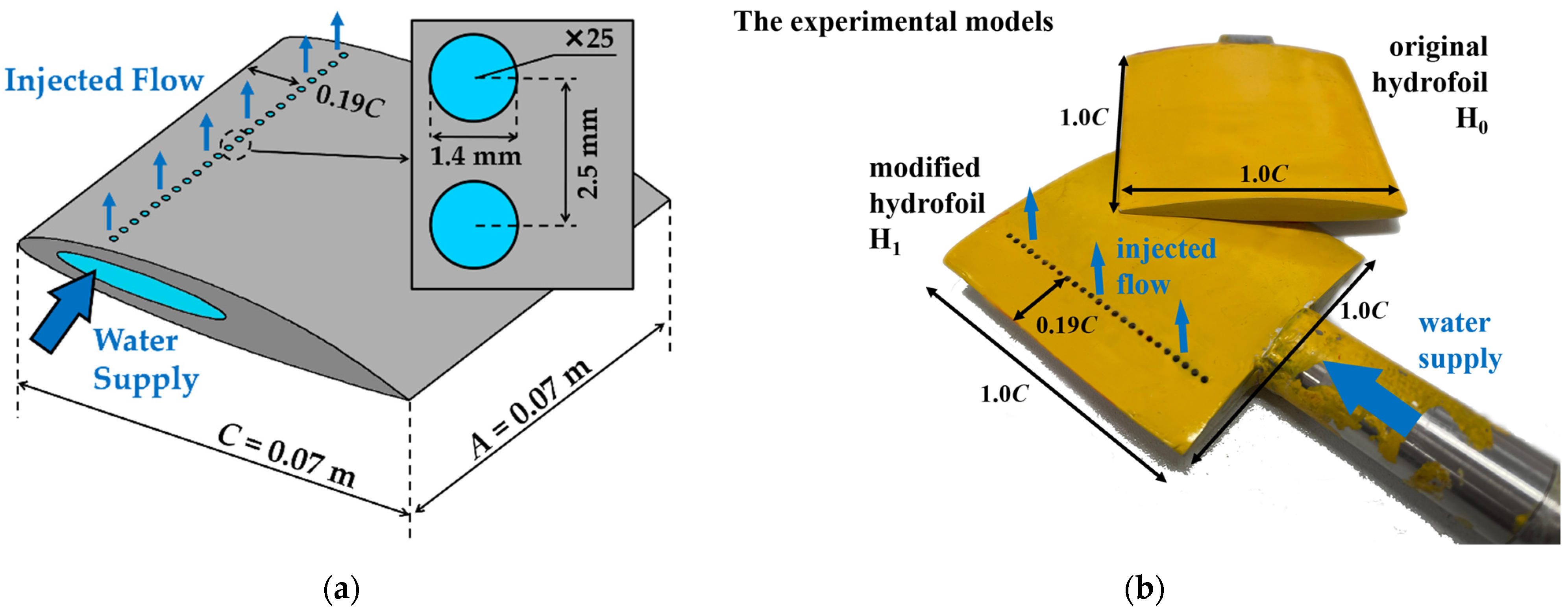
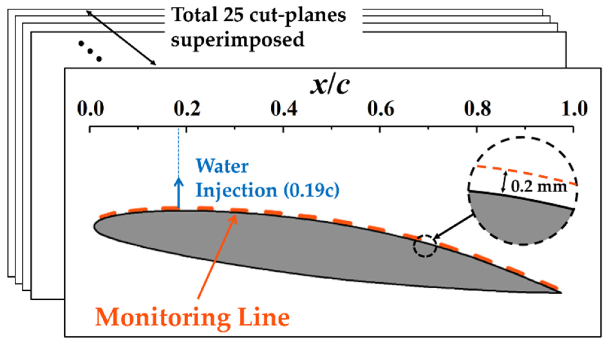
Figure 1 displays that 25 jet holes in line are set on the hydrofoil suction surface. Continuous water vertically jets out of the chamber (inside the hydrofoil) through the 25 equidistant distributed jet holes. The radius of each hole is r = 0.7 mm and the distance between each hole is ∆s = 2.5 mm. Both the chord length C and span length A of the hydrofoil are 0.07 m. The jet holes are located at 0.19C from the hydrofoil leading edge. The outlet velocity of jet holes is set as 3.25 m/s in this numerical calculation. The configuration mentioned above corresponds to our previous experiments [27].
2.2. Simulation Setup
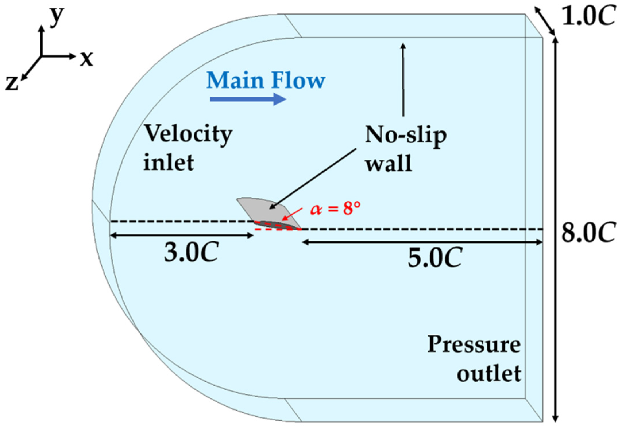
Figure 2 illustrates the configuration of the whole calculation domain. An NACA66 (MOD) hydrofoil (with the attack angle of α = 8°) is placed in the fluid domain. In order to guarantee the calculation stable, the inlet is set as 3.0C distance from the leading edge of the hydrofoil, and the outlet is 5.0C downstream the trailing edge. The inlet velocity is set as U∞ = 7.83 m/s, and the outlet boundary is chosen as P∞ = 27,325 Pa. The no-slip wall boundary conditions are applied on the hydrofoil surface and the tunnel wall. The water density is set as ρ = 998 kg/m3. The saturated vapor pressure is P* = 1940 Pa at the test temperature T = 17 °C. Consequently, the corresponding Reynolds number is 5.1 × 10⁵ and the cavitation number is σ = 0.83. The numerical configuration mentioned above also corresponds to our previous experiments [27].
2.3. Mesh Arrangement
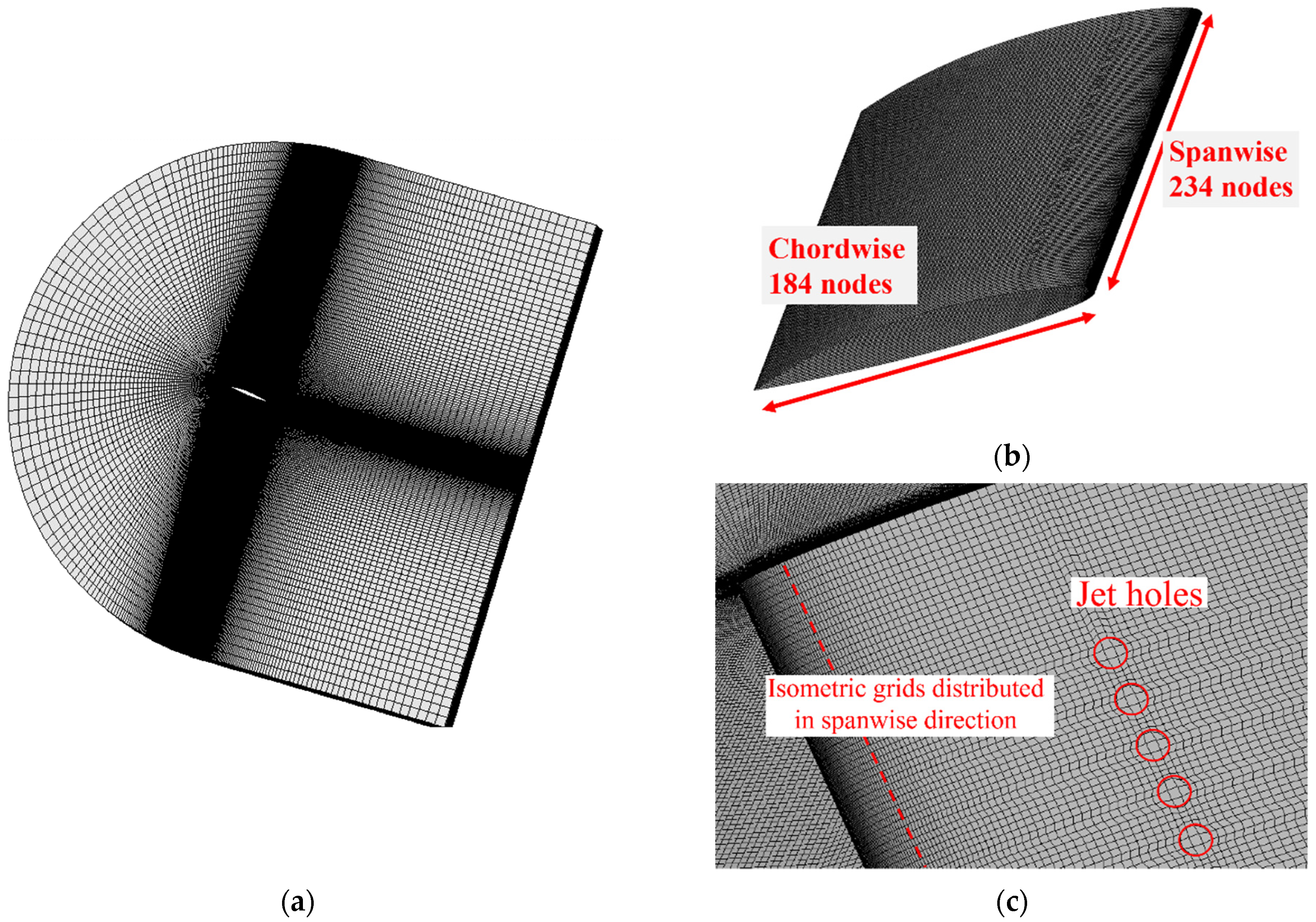
Figure 3 illustrates the hexahedral structured mesh obtained by the software of ICEM 19.2. Grids near the jet holes and the leading/trailing edge are refined, as shown in Figure 3b,c.
Table 1 gives the mesh independence results. The lift coefficient Cl, drag coefficient Cd and lift-drag ratio K = Cl/Cd are taken into evaluation. The values of Cl, Cd, and K tend to stay the same when the nodes number is 11,129,600; therefore, Mesh 2 is adopted in the following investigation. In Mesh 2, there are 184 nodes arranged along the chord direction and 234 nodes along the span direction. The values of y+ on the hydrofoil surface are within 0.5–2.
3. Numerical Methods
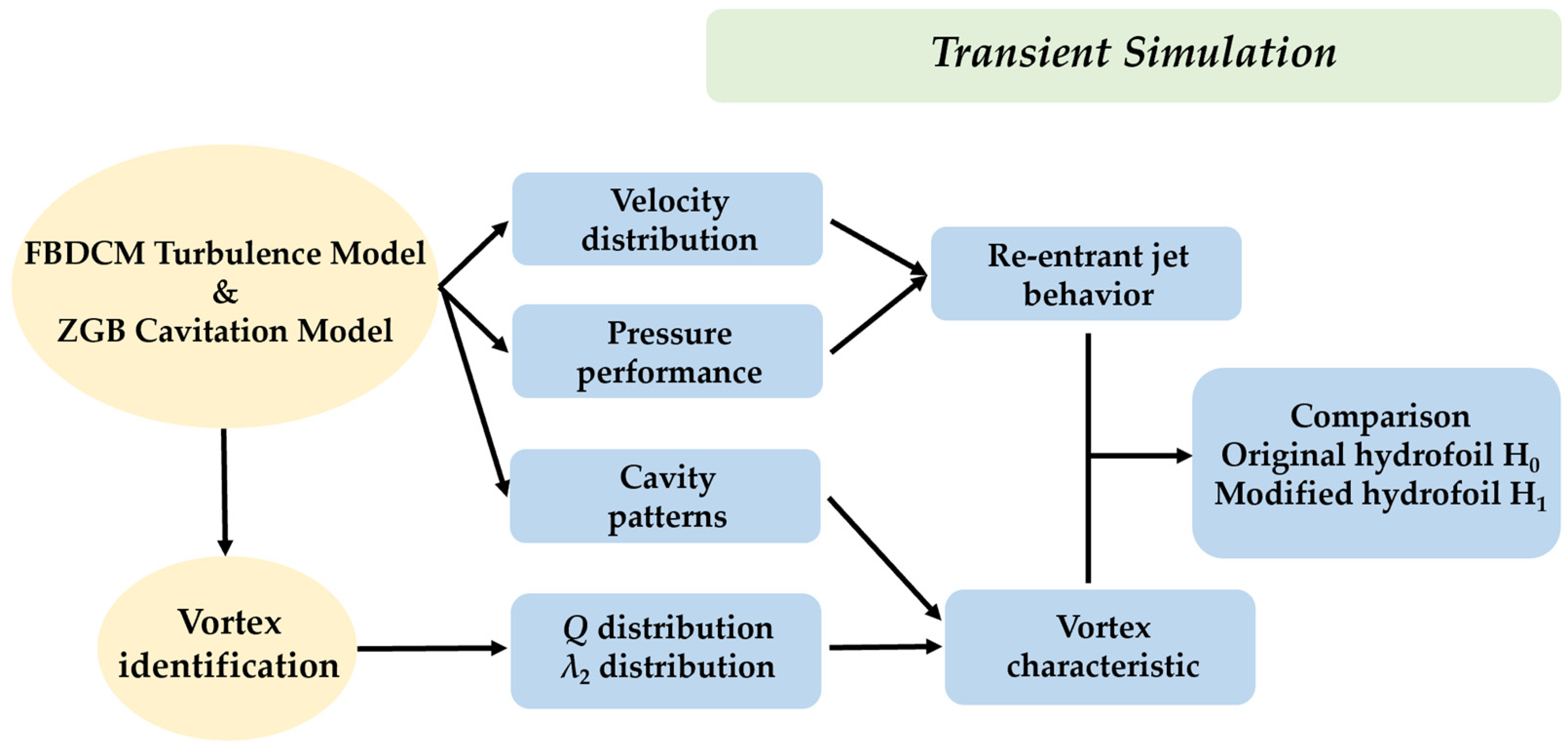
The software Fluent 19.2 is employed to obtain numerical calculation results. The turbulence model of FBDCM [34] and the cavitation model of ZGB [38] are adopted to obtain the transient cavitating flow characteristics. Considering the calculation time and solution accuracy, the time step is set as 0.5 ms. The calculated velocity and pressure distribution are analyzed to discuss the effect of water injection on the re-entrant jet behavior. Vortex identification methods, including Q criterion and λ2 criterion, are adopted to analyze the vortex motion characteristics in the near-wall region and in cavitating flow. Figure 4 shows the flowchart of numerical simulation in this paper. The original and modified hydrofoil are named H0 and H1 in short, respectively.
3.1. Turbulence Model
The governing equations are described as:
The governing equations are described as:
where ρm, µm, and µt are the mixed-phase density and mixed-phase laminar/turbulent viscosity coefficient, i and j represent the coordinate directions, and p and u are the pressure and velocity of the mixture phase, respectively. αv denotes the vapor volume fraction, l and v indicate the liquid and vapor phase, respectively.
According to the aforementioned literature about the turbulence model, the FBDCM turbulence model [34] is adopted to analyze the flow characteristics. Firstly, the turbulence viscosity of the standard k-ε turbulence model is:
where k represents the turbulence kinetic energy, and ε denotes the dissipation rate of turbulence kinetic energy, and the correction coefficient Cμ is set as 0.085 recommended in reference [48].
Then, based on the aforementioned standard k-ε turbulence model, the FBDCM model blends the FBM [32] (Equation (6)) and DCM [33] (Equation (7)) models according to the density of the local fluid. The fFBM and fDCM are the correction coefficients of the filtering model and the density correction model, respectively. In the FBDCM model, a function χ (ρm/ρl) is adopted to correct the turbulent viscosity μt of Equation (5), as shown below:
where C1 and C2 are constants, and the recommended values are C1 = 4 and C2 = 0.2 in literature [49]. The density correction factor n = 10 in Equation (7) recommended in literature [50] is adopted.
3.2. Cavitation Model
For the cavitation model, the ZGB model [38] is adopted in this numerical study. The model is based on the mass transport Equation (11), as follows:
where RB is the bubble radius (the reference value is 1 μm); the reference value of αnuc for nucleation amount is 5 × 10⁻⁴; Fvap is the evaporation coefficient (the reference value is 50); Fcond represents the condensation coefficient (the reference value is 0.01). Considering the influence of turbulent kinetic energy on cavitation, the saturated vapor pressure Pv is modified by Equation (14) in Equations (12) and (13).
3.3. Vortex Identification Methods
The tensor J of velocity gradient can be divided into the symmetric part: S (strain rate tensor) and the antisymmetric part: R (spin tensor). The formulas are as follow:
where U, V, and W are the velocities of the flow field relative to the three directions of Cartesian coordinate system x, y, and z, respectively.
Jeong et al. [50] believed that the minimum pressure caused by vortical flow is one of the necessary conditions for vortex determination. The tensor S2 + R2 has three real eigenvalues, and when there are two negative eigenvalues, there is a minimum value of pressure in the region. The symmetric tensor S2 + R2 contributes to vortex formation; that is, a region of S2 + R2 with two negative eigenvalues connected represents that there exist vortexes. When the second eigenvalue (λ2) of S2 + R2 is negative, the existence of vortexes is determined, namely the λ2 criterion:
Hunt et al. [51] defined the second matrix invariant Q of velocity gradient tensor J in the flow field. The region with Q positive value is determined as vortex existence [51]. The Q can be expressed as:
Researchers believe that the vortex shown by Q and λ2 methods can clearly reflect the vortex structures in cavitating flow [52,53,54]. The time Tc represents the time required for the main stream to flow through the chord length C of the hydrofoil.
In order to facilitate the discussion later, the values of Q and λ2 are conducted as dimensionless:
where C = 0.07 m is the hydrofoil chord length and U∞ = 7.83 m/s is the velocity of the main stream. These criteria can realize the recognition and visualization of vortex structures.
4. Simulation Validation
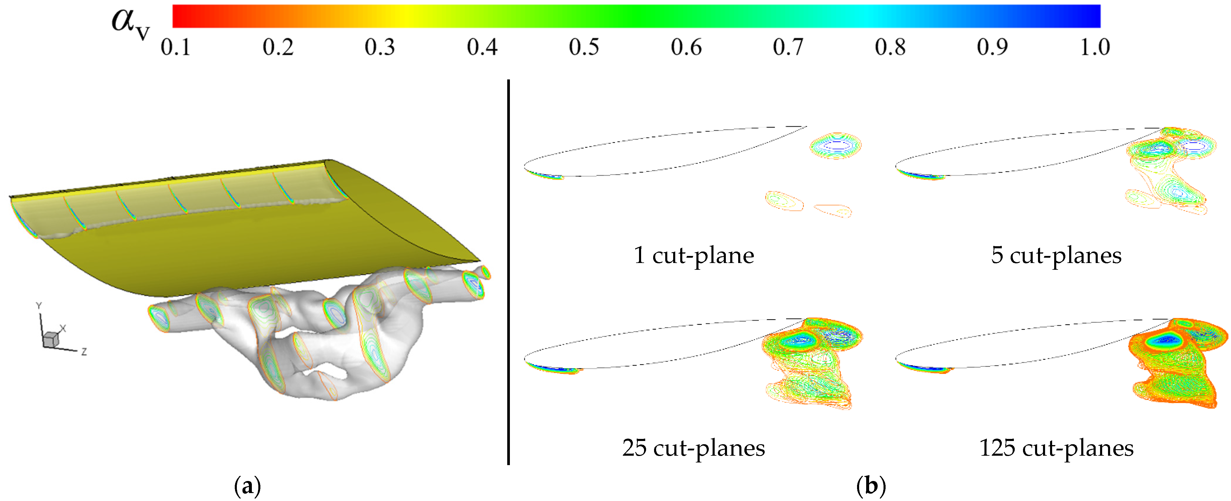
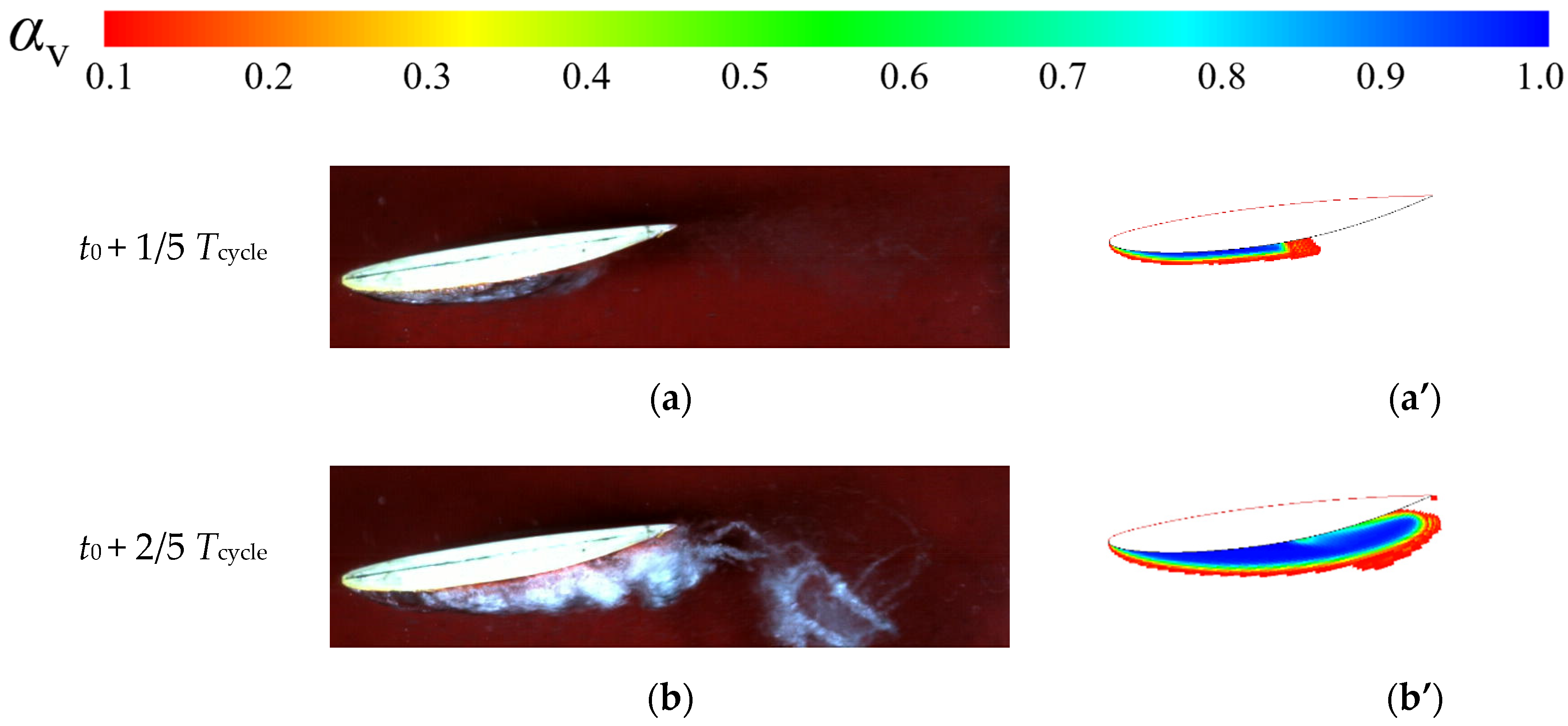
In order to verify the accuracy of the numerical method, the numerical calculation configuration of the same Reynolds number and cavitation number with that of the experiment [27] are compared. As shown in Figure 5a, 25 equidistant cut-planes in the hydrofoil span direction are extracted, and then superimposed to display the cavity patterns, which will ensure that the experimental results are as realistic as possible. Figure 5b indicates that the shape of cavitation tends to be stable as the number of cut-planes increases to 25. Figure 6a–e,a’–e’ show the cavity patterns at several moments in one periodical time Tcycle. The time-averaged cavity patterns are shown in Figure 6f,f’. It is observed that the numerical simulations are in good agreement with experimental observations.
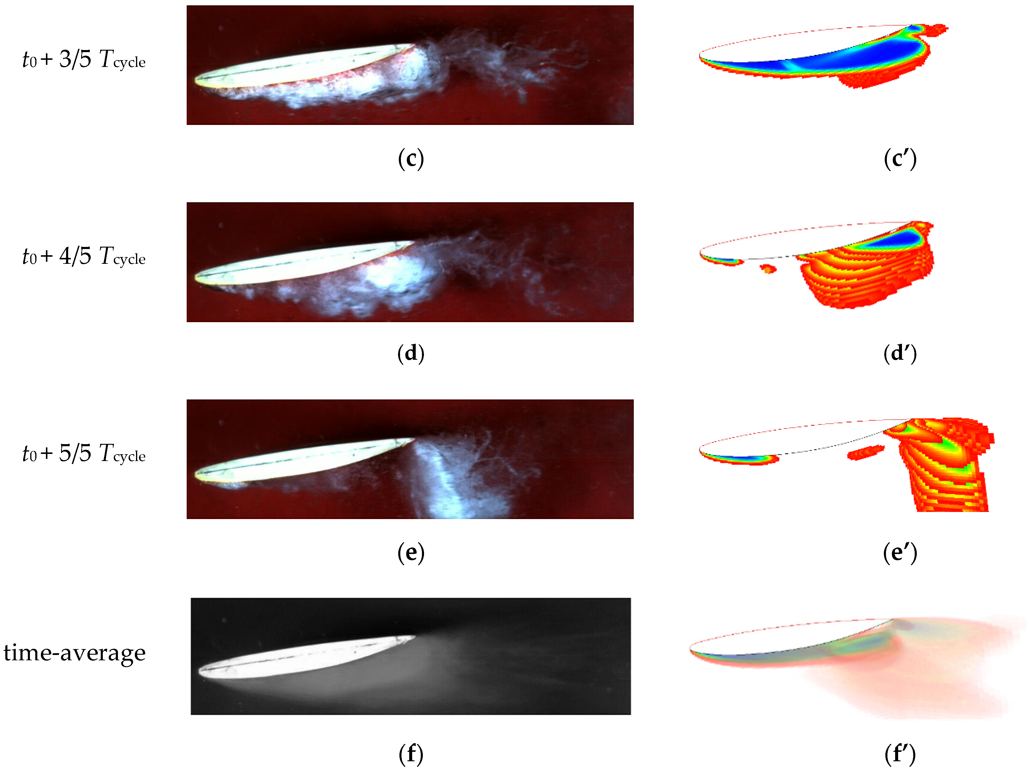
Figure 7 illustrates the dimensionless cavity area S/S0 quantitatively and shedding cycle for the numerical (0.5 ms time step) and experimental results in five cycles. The S0 is the cross-sectional area of the NACA66 (MOD) hydrofoil, and the cavity area S is normalized by area S0. The errors of the cavity shedding period and dimensionless cavitation area S/S0 are about 6.4% and 1.8%, respectively. A time step sensibility analysis is checked in Table 2. It can be seen that when the time step is set as 0.1 ms, the prediction accuracy is also relatively high; however, this configuration consumes a lot of computer resources. When the time step set as 0.5 ms, the prediction accuracy is close to that of 0.1 ms, and the error is within an acceptable range. Based on the above analysis, the mesh and numerical methods adopted in this paper are suitable and reasonable for calculating the flow field.
5. Results and Discussion
5.1. Vortex Performance
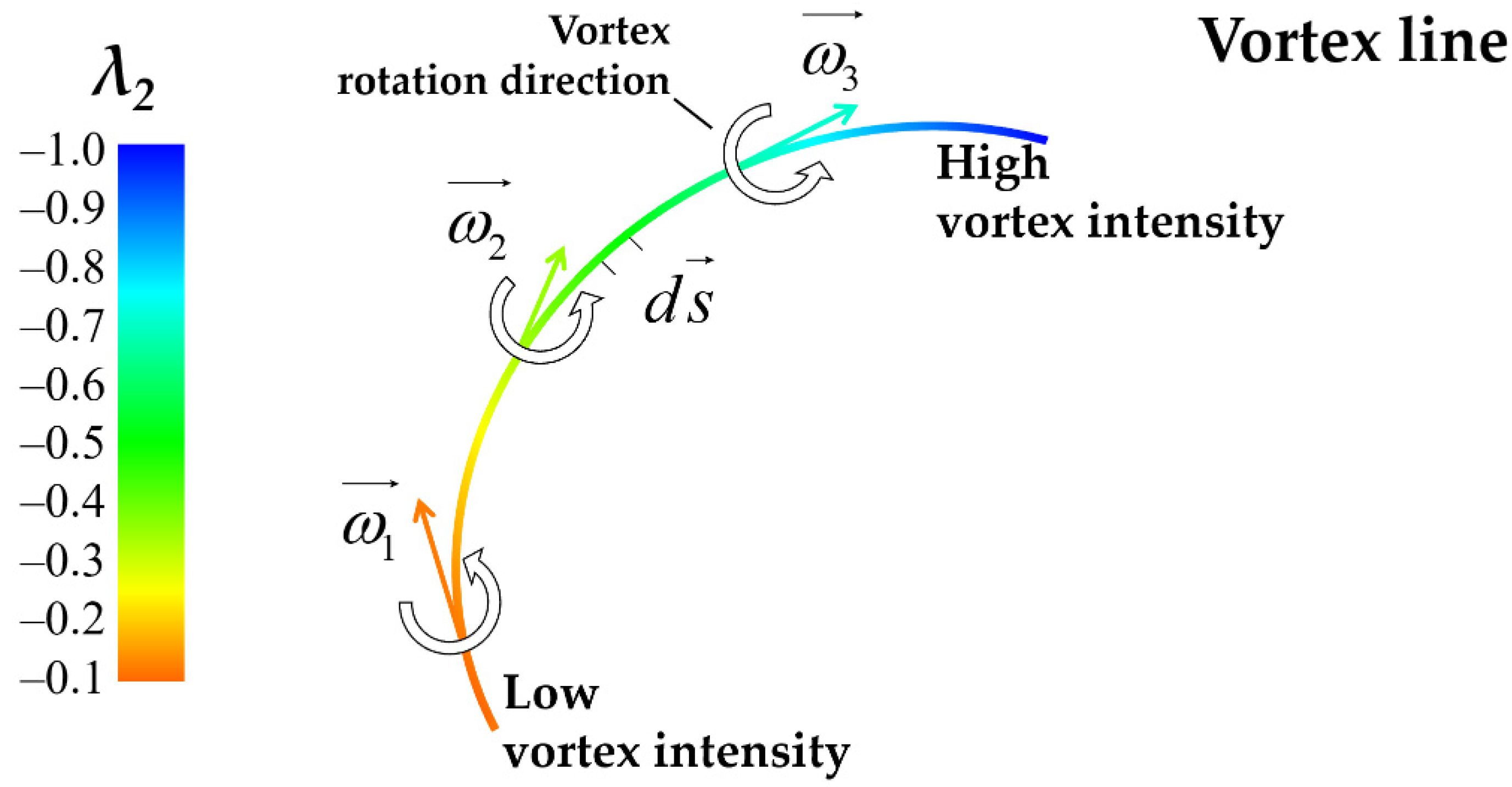
In order to describe the vortex visually and quantitatively, the vortex line coupled with the λ2 value is introduced. As shown in Figure 8, the tangent direction of a certain point on the vortex line is consistent with the vorticity direction at that point. The determination of the rotation direction is based on the right-hand rule: the direction pointed at by the right thumb is the vorticity direction of a certain point on the vortex line, and the direction of the other circling four fingers is the rotation direction of the vortex. The value of λ2 indicates the vortex intensity. The smaller the λ2 value, the higher the vortex intensity is.
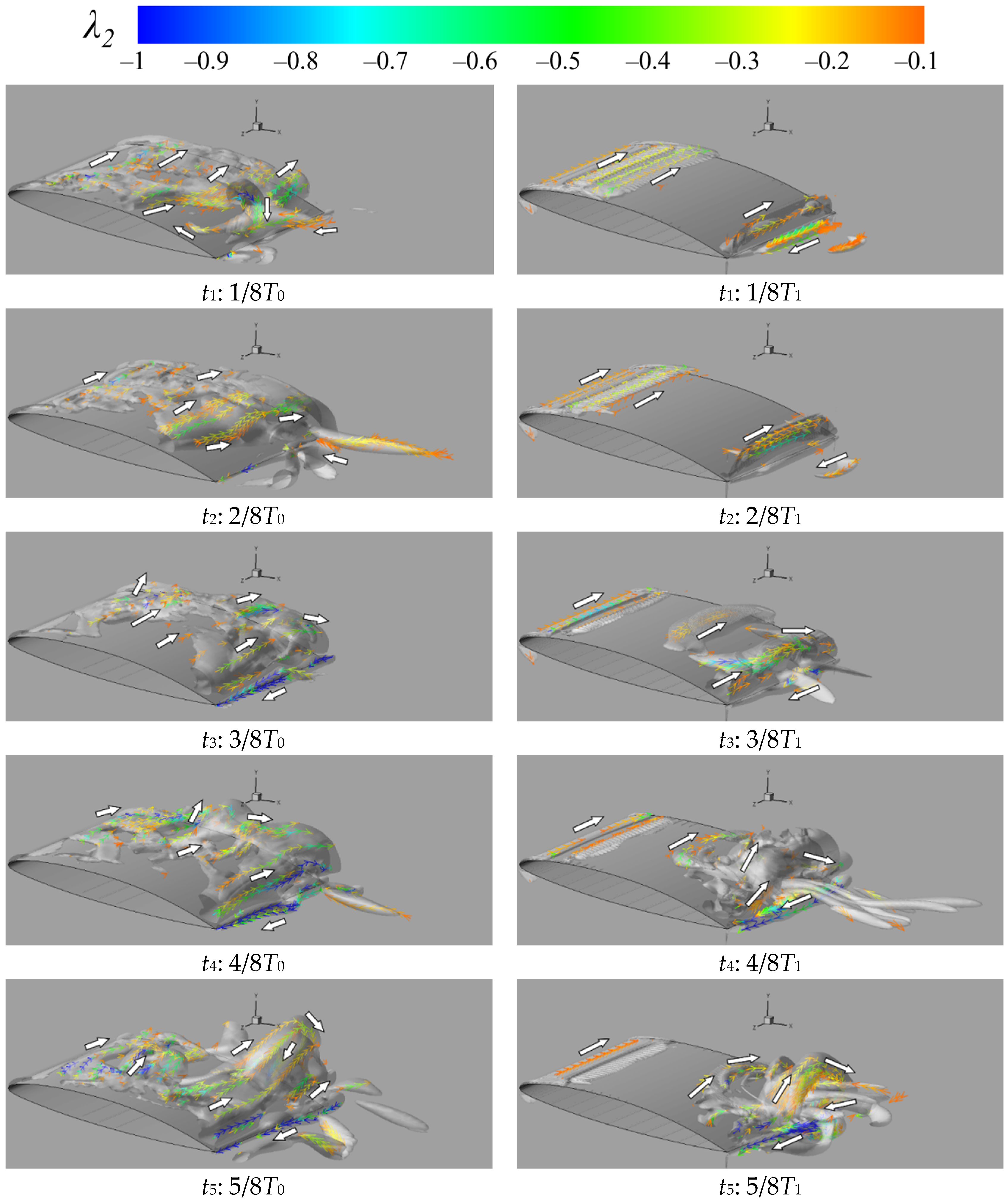
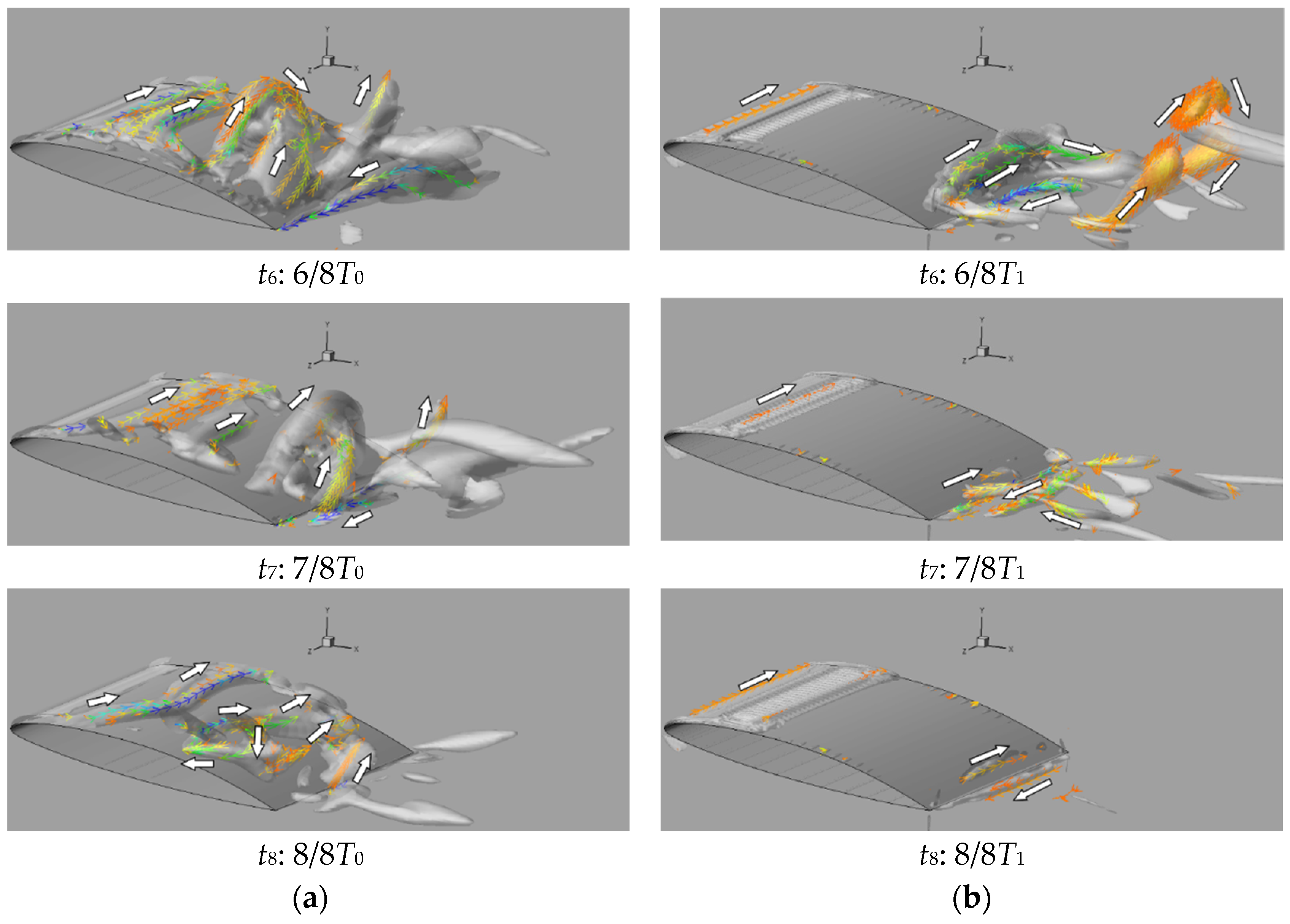
Figure 9 illustrates the distribution of vortex lines and the cavitation evolution process in one time cycle (cavity shape is defined by iso-surface of vapor volume fraction αv = 0.85). The period for H0 and H1 hydrofoil is indicated as T0 and T1, respectively. In order to observe more clearly, additional arrows are used to mark the main rotation direction of the vortexes in a certain region based on the right-hand rule. The lowest vortex intensity is shown in orange color and the highest vortex intensity is shown in blue color.
As shown in Figure 9a, vortex and cavity are interweaved all over above the suction surface of H0 during the entire period. The vortexes with different rotation directions are observed because the cavitation in the previous cycle causes unstable flow. The process from the moment t2 to t3 is the development stage of attached cavitation, and the vortex lines are mainly distributed along the −z-axis direction. The attached cavity rolls in the clockwise direction and moves downstream. At the t4 moment, the wide-range cloud cavity shedding appears near the trailing edge. From the moment t4 to t8, the cavitation evolution shows the process of shedding–expansion–collapse, and the vortex structures are complicated. In particular, the cavity at t8 moment even trends to rotate around the x-axis. It is worth mentioning that vortexes with high intensity rotate around the +z direction near the trailing edge from the moment t2 to t4. The reason is that the recirculating flow crossing the trailing edge supplies the re-entrant jet with energy and further causes serious cavity shedding.
Figure 9b illustrates that the water injection obviously suppresses cavitation and weakens vortex intensity. Different from the vortex structures covering all over the suction surface of original hydrofoil H0, only fewer vortexes cover the leading edge and trailing edge of the H1 hydrofoil. From the moment t1 to t3, the vortex intensity around H1 is observed to be much lower than that around H0, and the vortex lines are parallel to each other, indicating that the flow field is relatively stable. During the process from the moment t4 to t6, the cavity evolution also experiences the process of shedding–expansion–collapse, but the vortex generating area is much smaller than that of the original hydrofoil H0. Then, the flow field becomes stable again after the moment t7. Compared with H0, the vortex intensity near the trailing edge of H1 is reduced, showing that the strength of recirculating flow is weakened. We conclude that the vortex motion is closely related to the cavitating flow. The water injection significantly weakens the vortex intensity and reduces the vortex region; thereby, cloud cavitation is avoided.
5.2. Re-Entrant Jet Behavior
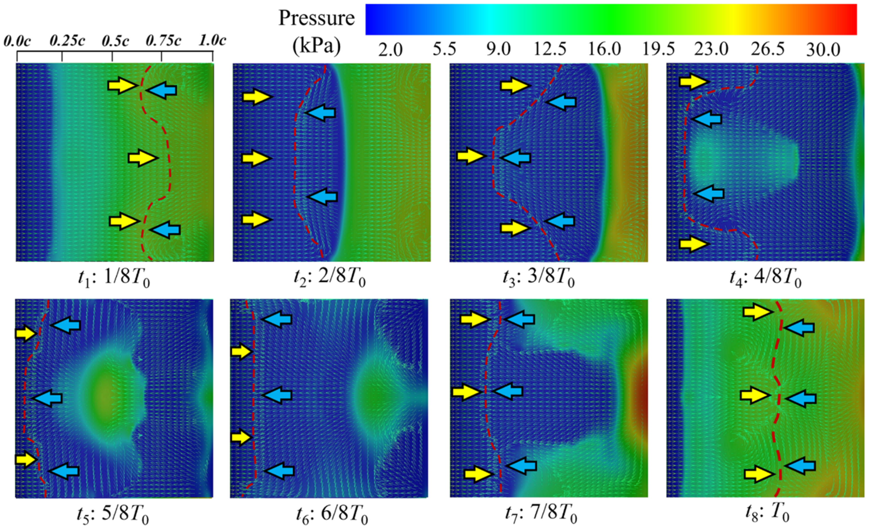
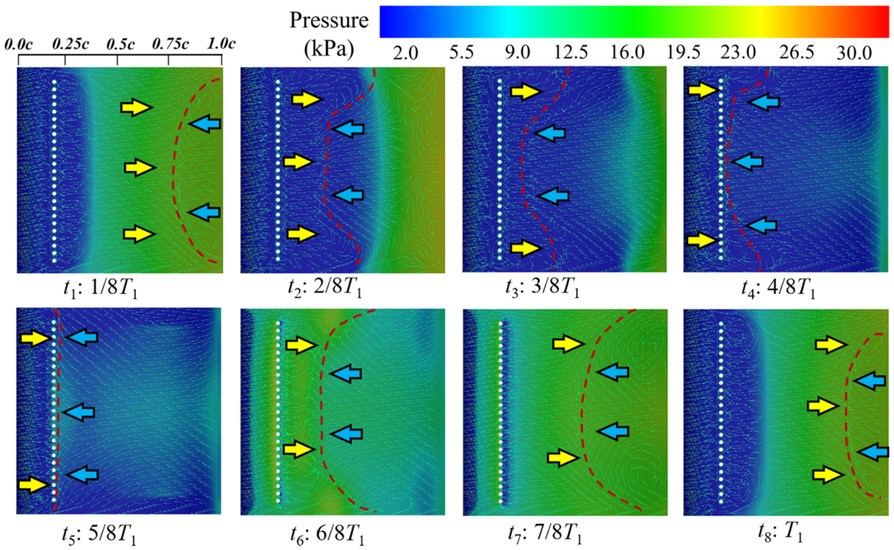
The re-entrant jet may cause cavity shedding and flow separation; however, water injection will change the re-entrant jet behavior. Figure 10 displays the velocity and pressure distributions on the suction surface of the original hydrofoil H0 in one period T0. In order to show more clearly, additional right-pointing arrows (in yellow color) are added in figures to represent the direction of the main flow, and the left-pointing arrows (in blue color) indicate the direction of the re-entrant jet. The added dotted lines mark the location where the two streams collide. At the moment of t1, the re-entrant jet interfaces with the mainstream at a distance of 0.6C from the leading edge. From t1 to t5, the re-entrant jet propagates upstream and reaches the farthest position (0.05C from the leading edge). At the moment of t5, the re-entrant jet is distributed almost all over the suction surface. Then starting from t7, the re-entrant jet gradually retracts and returns to 0.6C again at t8.
As shown in Figure 11, the average region of the re-entrant jet in an entire period for H1 is significantly reduced after the water injection. The re-entrant jet starts to propagate upstream at the moment of t1 and reaches the farthest position (near the jet holes at 0.2C) at t4. Starting from t5, the re-entrant jet begins to retract downstream. At t8, the re-entrant jet retreats to the position about 0.8C from the leading edge.
Based on the above analysis, the water injection is proved valuable to block the development of the re-entrant jet and shorten the duration of the low pressure on H1.
5.3. Relationship between Cavity and Re-Entrant Jet
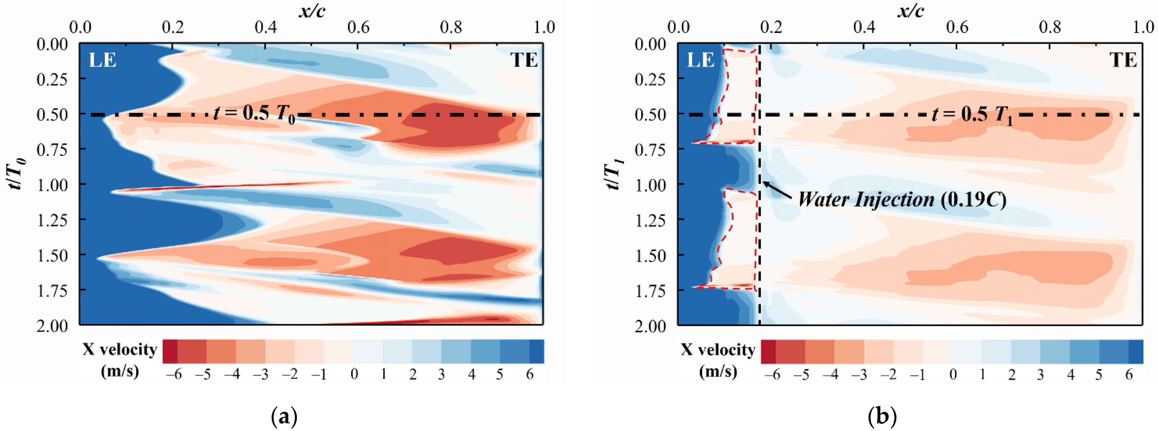
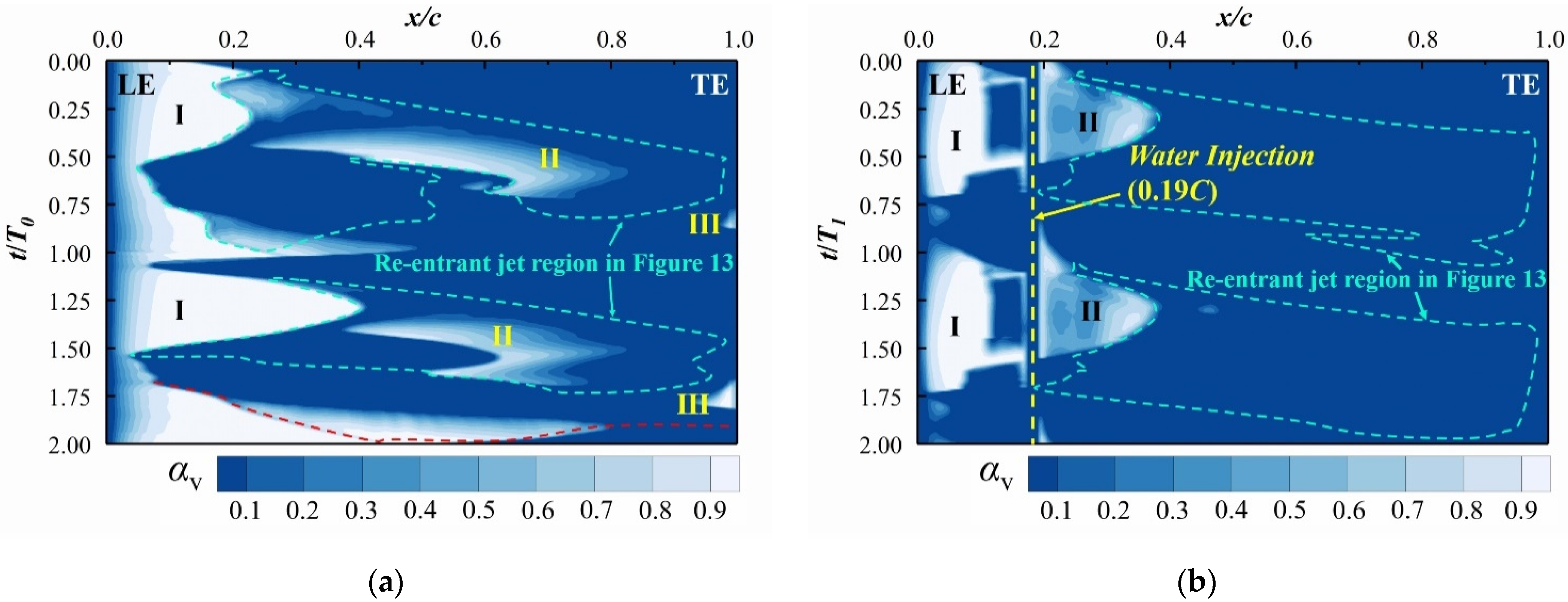
In order to discuss how the interaction of cavitation and re-entrant jet vary (after water injection adopted), a monitoring line is set near the hydrofoil suction surface, as shown in Figure 12. This kind of method is generally used to analyze the transient characteristics of cavitating flow in the near-wall region of hydrofoil [55,56]. The general idea can be described as: by adding the time dimension, the numerical results on the monitoring line are extracted and reconstructed to the two-dimensional flow field space–time contours of pressure, velocity, vapor fraction, etc. The monitoring line is set 0.2 mm away from the hydrofoil upper surface in this paper. The numerical results on the monitoring line are extracted from average data on 25 cut-planes (the configuration of the 25 cut-planes was described in the previous section).
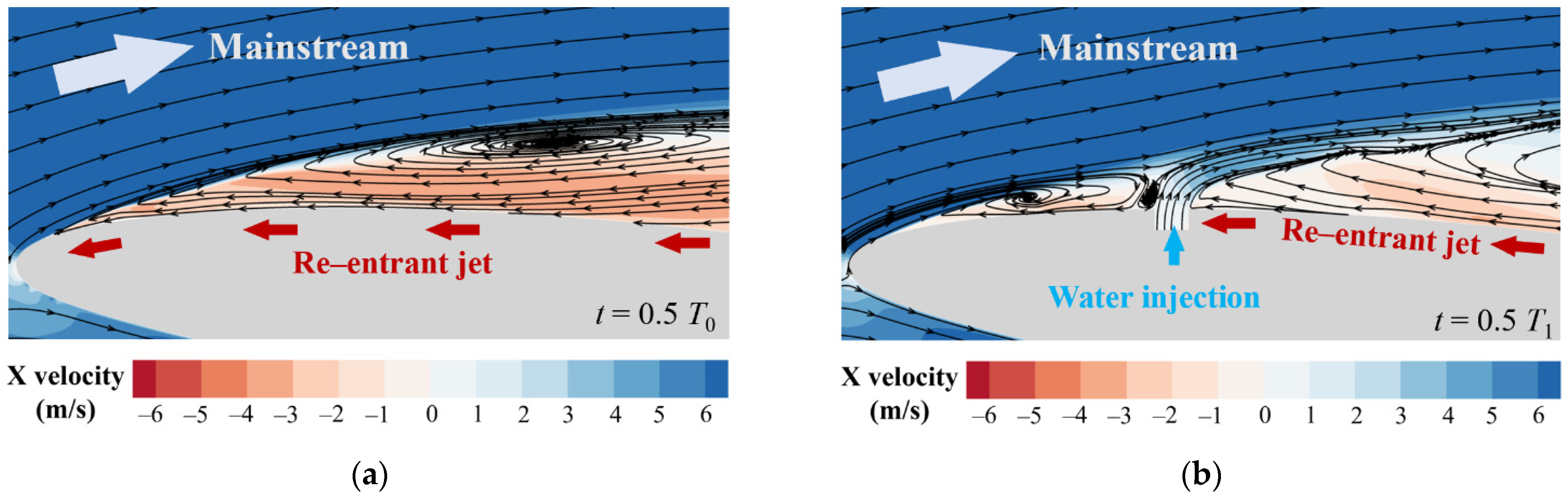
Figure 13 shows the contours of x-velocity as a function of space and time. The influence of water injection on the re-entrant jet intensity is quantitatively investigated. The re-entrant jet with high intensity is almost concentrated in the range of 0.5C–1.0C. The negative velocity of H0 reaches its maximum value of −6 m/s, observed in the range of 0.7C–0.9C. For H1, the injected water divides the negative velocity region into two parts. When the re-entrant jet propagates upstream near the jet hole (0.19C from the leading edge), its velocity gradually reduces to zero. Meanwhile, a region of negative X velocity appears again within the distance between 0.09C and 0.19C, as shown in the marked circles. This phenomenon can be explained by Figure 14, which shows the comparison of streamlines distribution at the midplane of H0 and H1 at the same corresponding time (0.5T0 for the original hydrofoil and 0.5T1 for the modified hydrofoil). For H0, the re-entrant jet propagates to the leading edge. For H1, the injected water flow is mixed with the main flow and then they flow downstream together; therefore, the re-entrant jet is resisted downstream of the jet hole and turns back and flows downstream together with the injected water flow and the main flow. It can also be seen from Figure 14b that a small incoming stream is blocked by the injected water flow and turns back to the leading edge, thus forming a small vortex structure. According to the numerical calculation results, the time-average velocity of the re-entrant jet in the near-wall region of H0 and H1 is −2.93 m/s and −1.55 m/s, respectively. The water injection reduces the re-entrant jet intensity by 46.98%.
Time evolution of vapor volume fraction αv as a function of space and time is shown in Figure 15. For the original hydrofoil H0, the near-wall cavitation can be divided into three parts: attached cavity region I (αv > 0.7), vapor–water mixing region II (αv < 0.7), and free cavity region III. As indicated in Figure 14b, the cavity area for H1 is significantly smaller than that of H0, and it is divided into parts I and II by the jet holes. Moreover, there is no free cavity region III (free cavity) observed near the trailing edge of H1, proving that water injection can suppress cavitating flow downstream. Combining Figure 13 and Figure 15 to observe the contour of re-entrant jet area and the shape of cavitation area, it is not difficult to find that the development of the re-entrant jet is responsible for triggering the cavity detachment [56], and hence resulting in an unsteady flow field.
5.4. Suppressing Mechanism
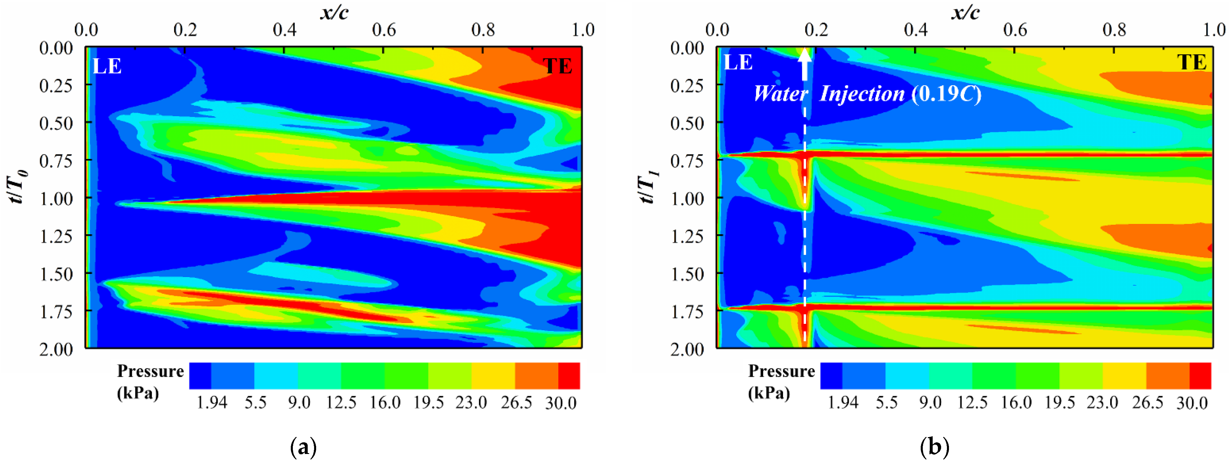
In this section, we first explore how the water injection inhibits the development of the re-entrant jet and weakens its intensity. Then, the internal mechanism of water injection on suppressing cloud cavitation is discussed. As shown in Figure 16, the outline of the low-pressure (less than the saturated pressure P* = 1940 Pa) region corresponds to the cavitation region in Figure 15. It can be seen that the low-pressure area for H0 is from 0.02C to 0.86C while 0.02C to 0.4C for H1. The water injection significantly reduces the low-pressure area, and therefore, suppresses the occurrence and development of cavitation fundamentally.
It is worth mentioning that the pressure variation from downstream to upstream of H0 shows more dramatic than that of H1. The adverse pressure gradient can lead to the production of vortex and re-entrant jet, which is the main cause of cloud cavity shedding [57]; therefore, it is worth exploring the influence of water injection on the pressure gradient near-wall. The local pressure coefficient and dimensionless pressure gradient are defined as:
where p represents the local pressure and p∞ denotes the far-field pressure.
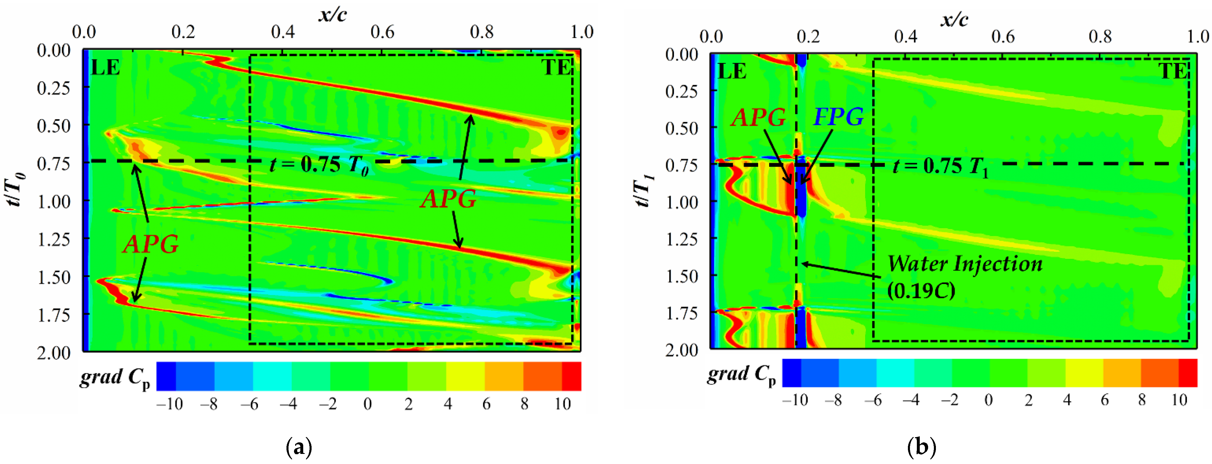
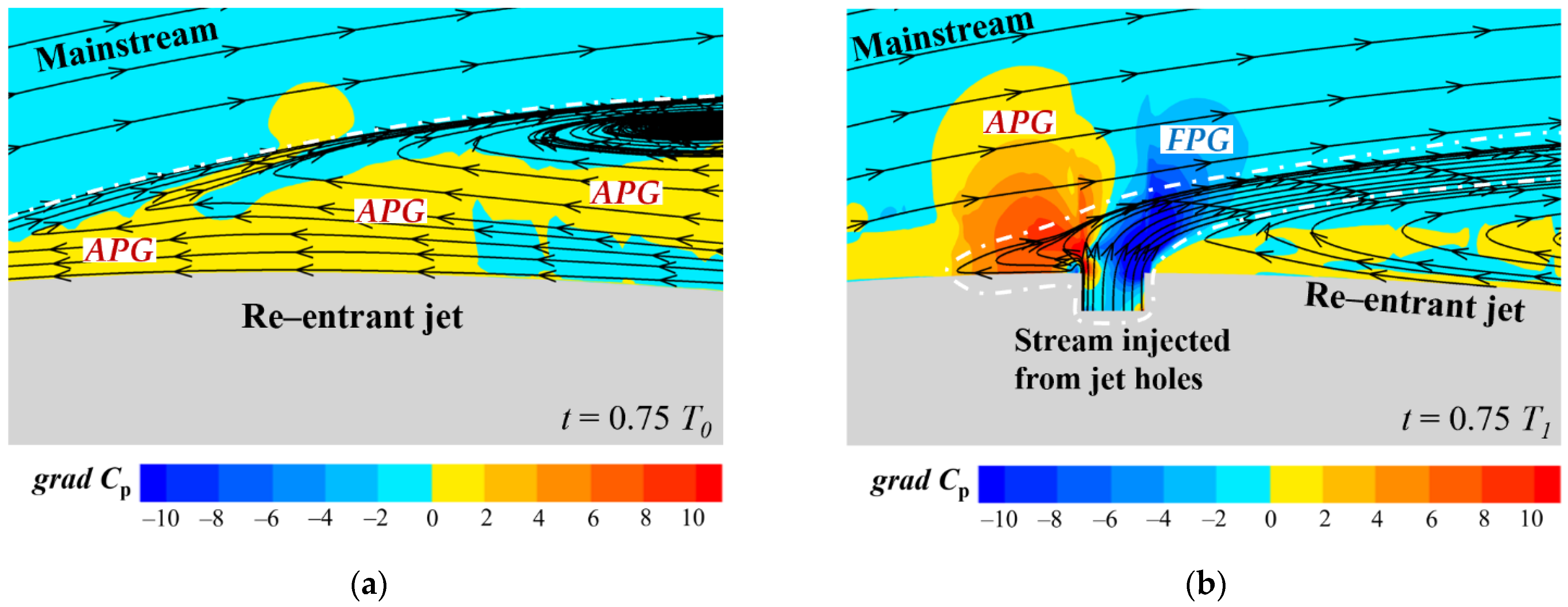
The positive value of gradCp in this paper represents the adverse pressure gradient (APG). APG makes the flow direction of the local fluid opposite to the mainstream, which is one of the main reasons for forming the re-entrant jet. The negative value of gradCp in this paper indicates the favorable pressure gradient (FPG) from the leading edge to the trailing edge. FPG makes the flow direction of the local fluid consistent with the mainstream. In Figure 13, re-entrant jet with high intensity is mainly concentrated in the range of 0.5C to 1.0C for H0, which corresponds to the high APG region in Figure 17. As shown in Figure 17b, the injected water generates high FPG downstream of the jet hole, which is this effect that resists the re-entrant jet propagating upstream. The pressure of the injected water flow is relatively high, which makes a high APG appear upstream of the jet holes, and thus a small range of negative velocity region appears, correspondingly, as shown in Figure 14b; therefore, this region is not defined as a “re-entrant jet”, because it is caused by the water injection. The re-entrant jet has been blocked by the FPG generated by the injected water flow. In order to understand the FPG generated by water injection more clearly, Figure 18 shows an enlarged view around the jet hole on the midplane of H1 (The corresponding position view of H0 is also displayed) at a certain moment (0.75T0 for H0 and 0.75T1 for H1). It can be seen from Figure 18b that a pair of APG and FPG appears above the jet hole. The FPG generated by water injection is higher than the APG in the re-entrant jet region, thus hindering the development of the re-entrant jet.
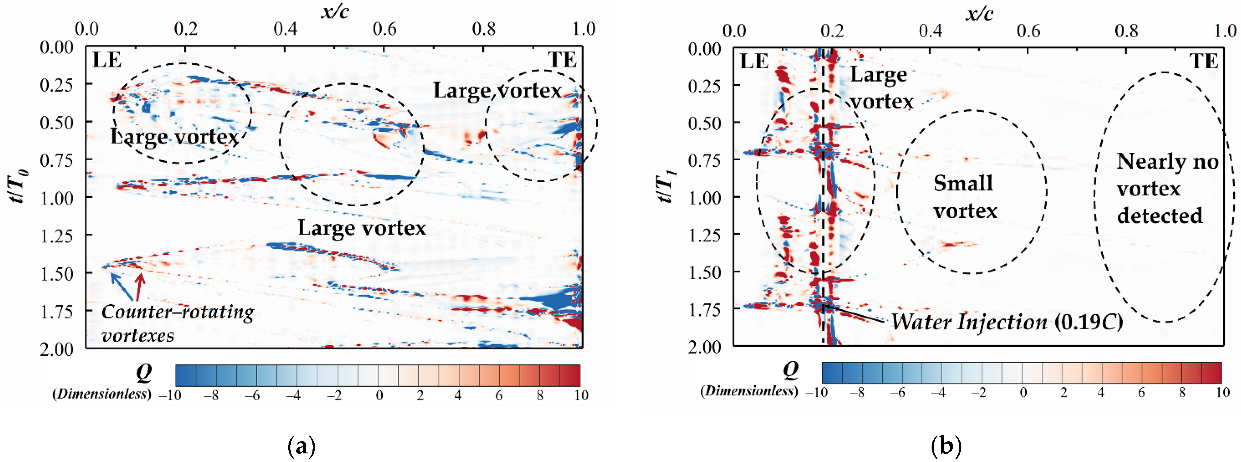
Figure 19 illustrates the distribution of Q values near the suction surface wall. The positive (in red color) and negative (in blue color) values indicate vortexes with opposite directions according to reference [36]. The vortex structures for H0 are distributed nearly all over the entire suction surface, while for H1, it is mainly concentrated on the leading edge and near the jet holes. As indicated in Figure 19b, the distribution area of Q is drastically reduced when the water injection is adopted. The injected water generates vortexes near the jet holes, making the position of the vortexes more forward than that of H0. From 0.4C to 1.0C, there are still large vortexes on H0, while small vortexes on H1, and there are almost no vortexes detected on H1 near the trailing edge. Vortex causes flow instability, and the water injection reduces vortexes, thus stabilizing the effect on the boundary layer.
Based on the above results, we can infer as follows: For H0, the shedding of large vortexes caused large-scale flow separation, which leads to the speed loss on the suction surface. The shedding vortexes transfer energy in the form of direct dissipation near the trailing edge of the hydrofoil. The kinetic energy of the vortex is converted into internal energy, resulting in an abrupt rise of pressure at the moment of cavity collapse, and hence unsteadiness. For H1, due to the mixing effect of the main flow, re-entrant jet, and attached cavity, the vortexes are generated near the jet holes and then directly dissipated nearby, instead of continuing to propagate to the trailing edge. The fluid kinetic energy near the hydrofoil wall is relatively low, while far away from the wall is larger. The water injection brings fluid kinetic energy to the near-wall region, which avoids large-scale separation of the boundary layer and stabilizes the entire flow field.
6. Conclusions
In this study, we conducted a computational investigation of the water injection method effect on suppressing vortical flow and re-entrant jet for a three-dimensional NACA66 hydrofoil under the cloud cavitation condition (σ = 0.83, Re = 5.1 × 10⁵). Based on the numerical results, the qualitative and quantitative analyses demonstrate that the proposed method can effectively hinder the re-entrant jet development and suppress the cloud cavitation and vortex. The detailed conclusions are summarized as follows:
- The water injection reduces the area of the low-pressure (<1940 Pa) region on the hydrofoil suction surface, thus suppressing the cavitation occurrence and development. The maximum range of low pressure is approximately 0.02C to 0.86C for H0 and 0.02C to 0.4C for H1, which is decreased by 54.76%. In the near-wall region of H1, the vapor–water mixing region II (αv < 0.7) shrinks significantly, and free cavity region III is no longer found.
- The vortexes are observed both inside the attached cavitation and the shedding cloud cavitation, and the water injection makes the vortex region shrink. The vortex structures above the suction surface of H1 are only distributed near the leading edge and trailing edge. Compared with H0, the λ2 values coupled on the vortex lines of H1 are relatively higher, indicating that the swirling strength is weakened.
- The water injection produces the FPGs locally, which hinders the propagation of the re-entrant jet and weakens its strength. For H0, the area of the re-entrant jet covers the entire suction surface at certain moments; For H1, when the re-entrant jet propagates to about 0.2C, it begins to retract. Compared with H0, the intensity of the re-entrant jet on the H1 suction surface is reduced by 46.98%. The water injected from jet holes itself has momentum, thus generating FPG. The water injection provides energy to the boundary layer, and hence steadiness the flow field; therefore, flow separation is suppressed.
- The vortex causes flow instability, and the water injection suppresses vortexes in the near-wall region, thus stabilizing the boundary layer. The Q distribution in the near-wall region indicates that vortexes are generated near the jet holes. For H0, the large vortexes are widely distributed from the leading edge to the trailing edge, and there are almost no vortexes in the range of 0.4–1.0C for H1.
Author Contributions
Methodology, Z.L. and W.W.; software, Z.L.; validation, Z.L.; formal analysis, Z.L.; investigation, Z.L. and W.W.; writing—original draft preparation, Z.L.; writing—review and editing, W.W. and X.J.; supervision, W.W. and X.W.; project administration, W.W.; funding acquisition, W.W. All authors have read and agreed to the published version of the manuscript.
Funding
This research was funded by the National Natural Science Foundation of China (51876022).
Institutional Review Board Statement
Not applicable.
Informed Consent Statement
Not applicable.
Data Availability Statement
The data from this study are not available for sharing.
Conflicts of Interest
The authors declare no conflict of interest.
References
- Ji, B.; Cheng, H.; Huang, B.; Luo, X.; Peng, X.; Long, X. Research Progresses and Prospects of Unsteady Hydrodynamics Characteristics for Cavitation. Adv. Mech. 2019, 49, 428–479. [Google Scholar] [CrossRef]
- Lei, T.; Shan, Z.B.; Liang, C.S.; Chuan, W.Y.; Bin Bin, W. Numerical simulation of unsteady cavitation flow in a centrifugal pump at off-design conditions. Proc. Inst. Mech. Eng. Part C J. Mech. Eng. Sci. 2013, 228, 1994–2006. [Google Scholar] [CrossRef]
- Tan, L.; Zhu, B.; Wang, Y.; Cao, S.; Gui, S. Numerical study on characteristics of unsteady flow in a centrifugal pump volute at partial load condition. Eng. Comput. 2015, 32, 1549–1566. [Google Scholar] [CrossRef]
- Li, D.-Q.; Grekula, M.; Lindell, P. Towards numerical prediction of unsteady sheet cavitation on hydrofoils. J. Hydrodyn. 2010, 22, 699–704. [Google Scholar] [CrossRef]
- Usta, O.; Korkut, E. Prediction of cavitation development and cavitation erosion on hydrofoils and propellers by Detached Eddy Simulation. Ocean Eng. 2019, 191, 106512. [Google Scholar] [CrossRef]
- Luo, X.-W.; Ji, B.; Tsujimoto, Y. A review of cavitation in hydraulic machinery. J. Hydrodyn. 2016, 28, 335–358. [Google Scholar] [CrossRef]
- Liu, Y.; Tan, L.; Wang, B. A Review of Tip Clearance in Propeller, Pump and Turbine. Energies 2018, 11, 2202. [Google Scholar] [CrossRef] [Green Version]
- Liu, Y.; Tan, L. Method of T shape tip on energy improvement of a hydrofoil with tip clearance in tidal energy. Renew. Energy 2019, 149, 42–54. [Google Scholar] [CrossRef]
- Timoshevskiy, M.V.; Zapryagaev, I.I.; Pervunin, K.S.; Maltsev, L.I.; Markovich, D.M.; Hanjalić, K. Manipulating cavitation by a wall jet: Experiments on a 2D hydrofoil. Int. J. Multiph. Flow 2018, 99, 312–328. [Google Scholar] [CrossRef]
- Che, B.; Cao, L.; Chu, N.; Likhachev, D.; Wu, D. Effect of obstacle position on attached cavitation control through response surface methodology. J. Mech. Sci. Technol. 2019, 33, 4265–4279. [Google Scholar] [CrossRef]
- Zhang, L.; Chen, M.; Shao, X. Inhibition of cloud cavitation on a flat hydrofoil through the placement of an obstacle. Ocean Eng. 2018, 155, 1–9. [Google Scholar] [CrossRef]
- Capurso, T.; Menchise, G.; Caramia, G.; Camporeale, S.; Fortunato, B.; Torresi, M. Investigation of a passive control system for limiting cavitation inside turbomachinery under different operating conditions. Energy Procedia 2018, 148, 416–423. [Google Scholar] [CrossRef]
- Kadivar, E.; Timoshevskiy, M.V.; Pervunin, K.S.; el Moctar, O. Cavitation control using Cylindrical Cavitating-bubble Generators (CCGs): Experiments on a benchmark CAV2003 hydrofoil. Int. J. Multiph. Flow 2019, 125, 103186. [Google Scholar] [CrossRef]
- Kadivar, E.; el Moctar, O.; Javadi, K. Stabilization of cloud cavitation instabilities using Cylindrical Cavitating-bubble Generators (CCGs). Int. J. Multiph. Flow 2019, 115, 108–125. [Google Scholar] [CrossRef]
- Che, B.; Wu, D. Study on Vortex Generators for Control of Attached Cavitation. In Fluids Engineering Division Summer Meeting; American Society of Mechanical Engineers: New York, NY, USA, 2017. [Google Scholar] [CrossRef]
- Schmidt, S.J.; Likhachev, D. Control effect of micro vortex generators on leading edge of attached cavitation. Phys. Fluids 2019, 31, 044102. [Google Scholar] [CrossRef]
- Liu, Y.; Tan, L. Influence of C groove on suppressing vortex and cavitation for a NACA0009 hydrofoil with tip clearance in tidal energy. Renew. Energy 2019, 148, 907–922. [Google Scholar] [CrossRef]
- Liu, Y.; Tan, L. Method of C groove on vortex suppression and energy performance improvement for a NACA0009 hydrofoil with tip clearance in tidal energy. Energy 2018, 155, 448–461. [Google Scholar] [CrossRef]
- Wang, W.; Li, Z.; Liu, M.; Ji, X. Influence of water injection on broadband noise and hydrodynamic performance for a NACA66 (MOD) hydrofoil under cloud cavitation condition. Appl. Ocean Res. 2021, 115, 102858. [Google Scholar] [CrossRef]
- Wang, C.Z. Cavity Flow Mechanism Analysis and Passive Flow Control Technology Research; Dalian University of Technology: Dalian, China, 2013. [Google Scholar]
- Maltsev, L.I.; Dimitrov, V.D.; Milanov, E.M.; Zapryagaev, I.I.; Timoshevskiy, M.V.; Pervunin, K.S. Jet Control of Flow Separation on Hydrofoils: Performance Evaluation Based on Force and Torque Measurements. J. Eng. Thermophys. 2020, 29, 424–442. [Google Scholar] [CrossRef]
- De Giorgi, M.G.; Ficarella, A.; Fontanarosa, D. Active Control of Unsteady Cavitating Flows in Turbomachinery. In Turbo Expo: Power for Land, Sea, and Air; American Society of Mechanical Engineers: New York, NY, USA, 2019. [Google Scholar] [CrossRef]
- Timoshevskiy, M.V.; Zapryagaev, I.I. Generation of a Wall Jet to Control Unsteady Cavitation over a 2D Hydrofoil: Visualization and Hydroacoustic Signal Analysis. Proc. J. Phys. Conf. Ser. 2017, 899, 32021. [Google Scholar] [CrossRef] [Green Version]
- Timoshevskiy, M.; Zapryagaev, I.; Pervunin, K.; Markovich, D.M. Cavitation control on a 2D hydrofoil through a continuous tangential injection of liquid: Experimental study. In Proceedings of the AIP Conference Proceedings; Fomin, V., Ed.; American Institute of Physics: Melville, NY, USA, 2016; Volume 1770, p. 030026. [Google Scholar]
- Timoshevskiy, M.V.; Zapryagaev, I.I.; Pervunin, K.S.; Markovich, D.M. Cavitating flow control through continuous tangential mass injection on a 2D hydrofoil at a small attack angle. MATEC Web Conf. 2016, 84, 00039. [Google Scholar] [CrossRef] [Green Version]
- Timoshevskiy, M.V.; Zapryagaev, I.I.; Pervunin, K.S.; Maltsev, L.I.; Markovich, D.M.; Hanjalic, K. Cavitation Control on a Two-Dimensional Hydrofoil by Means of Continuous Tangential Injection. In Proceedings of the Bulletin of the Tomsk Polytechnic University, Geo Assets Engineering; AIP Publishing LLC: Melville, NY, USA, 2016; Volume 327, pp. 75–90. [Google Scholar]
- Lu, S.; Wang, W.; Hou, T.; Zhang, M.; Jiao, J.; Zhang, Q.; Wang, X. Experiment Research on Cavitation Control by Active Injection. In Proceedings of the 10th International Symposium on Cavitation (CAV2018); ASME Press: New York, NY, USA, 2019; pp. 363–368. [Google Scholar]
- Wang, W.; Tang, T.; Zhang, Q.D.; Wang, X.F.; An, Z.Y.; Tong, T.H.; Li, Z.J. Effect of water injection on the cavitation control:experiments on a NACA66 (MOD) hydrofoil. Acta Mech. Sin. 2020, 36, 999–1017. [Google Scholar] [CrossRef]
- Lee, C.-S.; Ahn, B.-K.; Han, J.-M.; Kim, J.-H. Propeller tip vortex cavitation control and induced noise suppression by water injection. J. Mar. Sci. Technol. 2017, 23, 453–463. [Google Scholar] [CrossRef]
- Huang, B.; Zhao, Y.; Wang, G. Large Eddy Simulation of turbulent vortex-cavitation interactions in transient sheet/cloud cavitating flows. Comput. Fluids 2014, 92, 113–124. [Google Scholar] [CrossRef]
- Zhang, Y.; Chen, K.; You, Y.; Sheng, L. Bouncing Behaviors of a Buoyancy-Driven Bubble on a Horizontal Solid Wall. Lixue Xuebao/Chin. J. Theor. Appl. Mech. 2019, 51, 1285–1295. [Google Scholar] [CrossRef]
- Johansen, S.T.; Wu, J.; Shyy, W. Filter-based unsteady RANS computations. Int. J. Heat Fluid Flow 2004, 25, 10–21. [Google Scholar] [CrossRef]
- Emvin, P.; Davidson, L.; Coutier-Delgosha, O.; Reboud, J.L.; Delannoy, Y. A local mesh refinement algorithm applied to turbulent flow. Int. J. Numer. Methods Fluids 1997, 24, 519–530. [Google Scholar] [CrossRef]
- Huang, B.; Wang, G.-Y.; Zhao, Y. Numerical simulation unsteady cloud cavitating flow with a filter-based density correction model. J. Hydrodyn. 2014, 26, 26–36. [Google Scholar] [CrossRef]
- Yu, A.; Ji, B.; Huang, R.; Zhang, Y.; Zhang, Y.; Luo, X. Cavitation shedding dynamics around a hydrofoil simulated using a filter-based density corrected model. Sci. China Ser. E Technol. Sci. 2015, 58, 864–869. [Google Scholar] [CrossRef]
- Cheng, H.; Long, X.-P.; Ji, B.; Liu, Q.; Bai, X.-R. 3-D Lagrangian-based investigations of the time-dependent cloud cavitating flows around a Clark-Y hydrofoil with special emphasis on shedding process analysis. J. Hydrodyn. 2018, 30, 122–130. [Google Scholar] [CrossRef]
- Long, X.; Cheng, H.; Ji, B.; Arndt, R.E. Numerical investigation of attached cavitation shedding dynamics around the Clark-Y hydrofoil with the FBDCM and an integral method. Ocean Eng. 2017, 137, 247–261. [Google Scholar] [CrossRef]
- Zwart, P.J.; Gerber, A.G.; Belamri, T. A Two-Phase Flow Model for Predicting Cavitation Dynamics. In Proceedings of the Fifth International Conference on Multiphase Flow, Yokohama, Japan, 30 May–4 June 2004; Volume 152, p. 152. [Google Scholar]
- Kawanami, Y.; Kato, H.; Yamaguchi, H.; Tanimura, M.; Tagaya, Y. Mechanism and Control of Cloud Cavitation. J. Fluids Eng. 1997, 119, 788–794. [Google Scholar] [CrossRef]
- Callenaere, M.; Franc, J.-P.; Michel, J.-M.; Riondet, M. The cavitation instability induced by the development of a re-entrant jet. J. Fluid Mech. 2001, 444, 223–256. [Google Scholar] [CrossRef]
- Ji, B.; Luo, X.; Wu, Y.; Peng, X.; Duan, Y. Numerical analysis of unsteady cavitating turbulent flow and shedding horse-shoe vortex structure around a twisted hydrofoil. Int. J. Multiph. Flow 2013, 51, 33–43. [Google Scholar] [CrossRef] [Green Version]
- Wang, Z.; Huang, B.; Zhang, M.; Wang, G.; Zhao, X. Experimental and numerical investigation of ventilated cavitating flow structures with special emphasis on vortex shedding dynamics. Int. J. Multiph. Flow 2018, 98, 79–95. [Google Scholar] [CrossRef]
- Zhang, Y.; Liu, K.; Xian, H.; Du, X. A review of methods for vortex identification in hydroturbines. Renew. Sustain. Energy Rev. 2018, 81, 1269–1285. [Google Scholar] [CrossRef]
- Ji, B.; Luo, X.; Arndt, R.E.; Peng, X.; Wu, Y. Large Eddy Simulation and theoretical investigations of the transient cavitating vortical flow structure around a NACA66 hydrofoil. Int. J. Multiph. Flow 2015, 68, 121–134. [Google Scholar] [CrossRef] [Green Version]
- Wang, C.-C.; Huang, B.; Wang, G.-Y.; Duan, Z.-P.; Ji, B. Numerical simulation of transient turbulent cavitating flows with special emphasis on shock wave dynamics considering the water/vapor compressibility. J. Hydrodyn. 2018, 30, 573–591. [Google Scholar] [CrossRef]
- Ganesh, H.; Makiharju, S.; Ceccio, S.L. Bubbly shock propagation as a mechanism for sheet-to-cloud transition of partial cavities. J. Fluid Mech. 2016, 802, 37–78. [Google Scholar] [CrossRef] [Green Version]
- Wang, C.; Huang, B.; Wang, G.; Zhang, M.; Ding, N. Unsteady pressure fluctuation characteristics in the process of breakup and shedding of sheet/cloud cavitation. Int. J. Heat Mass Transf. 2017, 114, 769–785. [Google Scholar] [CrossRef]
- Yakhot, V.; Orszag, S.A.; Thangam, S.; Gatski, T.B.; Speziale, C.G. Development of turbulence models for shear flows by a double expansion technique. Phys. Fluids A Fluid Dyn. 1992, 4, 1510–1520. [Google Scholar] [CrossRef] [Green Version]
- Coutier-Delgosha, O.; Fortes-Patella, R.; Reboud, J.L. Evaluation of the Turbulence Model Influence on the Numerical Simu-lations of Unsteady Cavitation. Proc. ASME Fluids Eng. Div. Summer Meet. 2003, 1, 341–346. [Google Scholar]
- Jeong, J.; Hussain, F. On the identification of a vortex. J. Fluid Mech. 1995, 285, 69–94. [Google Scholar] [CrossRef]
- Hunt, J.C.R.; Wray, A.A.; Moin, P. Eddies, Streams, and Convergence Zones in Turbulent Flows. Stud. Turbul. Using Numer. Simul. Databases-I1 1988, 193, 193–208. Available online: https://web.stanford.edu/group/ctr/Summer/201306111537.pdf (accessed on 12 August 2021).
- Arakeri, V.H.; Acosta, A.J. Viscous Effects in the Inception of Cavitation on Axisymmetric Bodies; ASME Pap: New York, NY, USA, 1973. [Google Scholar]
- Belahadji, B.; Franc, J.-P.; Michel, J.-M. Cavitation in the rotational structures of a turbulent wake. J. Fluid Mech. 1995, 287, 383–403. [Google Scholar] [CrossRef]
- Huang, B.; Wang, G. Experimental and numerical investigation of unsteady cavitating flows through a 2D hydrofoil. Sci. China Ser. E Technol. Sci. 2011, 54, 1801–1812. [Google Scholar] [CrossRef]
- Wang, G.; Wu, Q.; Huang, B. Dynamics of Cavitation–Structure Interaction. Acta Mech. Sin. 2017, 33, 685–708. [Google Scholar] [CrossRef]
- Huang, B.; Young, Y.L.; Wang, G.; Shyy, W.; Huang, B. Combined Experimental and Computational Investigation of Unsteady Structure of Sheet/Cloud Cavitation. J. Fluids Eng. 2013, 135, 071301. [Google Scholar] [CrossRef]
- Chen, Y.; Chen, X.; Gong, Z.; Li, J.; Lu, C. Numerical investigation on the dynamic behavior of sheet/cloud cavitation regimes around hydrofoil. Appl. Math. Model. 2016, 40, 5835–5857. [Google Scholar] [CrossRef]
Figure 1.
Introduction to the water injection method: (a) the modified hydrofoil model used in this numerical simulation; (b) the hydrofoil models used in our previous experiments [27,28].

Figure 2.
View of the computational domain.

Figure 3.
Mesh distribution: (a) the whole mesh domain; (b) grid distribution on the hydrofoil; (c) grid near the leading edge.
Figure 3.
Mesh distribution: (a) the whole mesh domain; (b) grid distribution on the hydrofoil; (c) grid near the leading edge.

Figure 4.
Flowchart of numerical study in this study.

Figure 5.
The influence of configurations of cut-plane numbers on the numerical results: (a) schematic diagram of the three-dimensional cavity shape; (b) the distribution of cavity patterns for different configurations of cut-plane numbers.
Figure 5.
The influence of configurations of cut-plane numbers on the numerical results: (a) schematic diagram of the three-dimensional cavity shape; (b) the distribution of cavity patterns for different configurations of cut-plane numbers.

Figure 6.
Comparison of cavity patterns [27] of experiment (left) with the numerical simulations (right), (a–e): Experimental observasions in one time cycle Tcycle. (a’–e’): Numerical results in the same one time cycle Tcycle. (f,f’): Time-averaged images for experiment [27] and simulation, respectively. (σ = 0.83, Re = 5.1 × 10⁵).


Figure 7.
Comparison of dimensionless cavitation area evolution [27]. (σ = 0.83, Re = 5.1 × 10⁵).
Figure 7.
Comparison of dimensionless cavitation area evolution [27]. (σ = 0.83, Re = 5.1 × 10⁵).

Figure 8.
Schematic diagram of the vortex intensity distribution and vortex direction.

Figure 9.
Distribution of vortex lines and cavity patterns (defined by iso-surface αv = 0.85) in a complete cycle: (a) original hydrofoil H0; (b) modified hydrofoil H1.
Figure 9.
Distribution of vortex lines and cavity patterns (defined by iso-surface αv = 0.85) in a complete cycle: (a) original hydrofoil H0; (b) modified hydrofoil H1.


Figure 10.
Distributions of velocity and pressure on the suction surface of H0 in one period T0.

Figure 11.
Distributions of velocity and pressure on the suction surface of H1 in one period T1.

Figure 12.
Schematic diagram of near-wall monitoring line.

Figure 13.
Time evolution of x-velocity on the monitoring line in two cycles for: (a) H0; (b) H1.

Figure 14.
Schematic of Streamlines and X velocity contours near the boundary layer of the leading edge at time 0.5T0 and 0.5T1 for: (a) H0; (b) H1, respectively.
Figure 14.
Schematic of Streamlines and X velocity contours near the boundary layer of the leading edge at time 0.5T0 and 0.5T1 for: (a) H0; (b) H1, respectively.

Figure 15.
Time evolution of vapor volume fraction αv on the monitoring line in two cycles for: (a) H0; (b) H1.
Figure 15.
Time evolution of vapor volume fraction αv on the monitoring line in two cycles for: (a) H0; (b) H1.

Figure 16.
Time evolution of pressure on the monitoring line in two cycles for: (a) H0; (b) H1.

Figure 17.
Time evolution of dimensionless pressure gradient on the monitoring line in two cycles for: (a) H0; (b) H1.
Figure 17.
Time evolution of dimensionless pressure gradient on the monitoring line in two cycles for: (a) H0; (b) H1.

Figure 18.
Zoom view of streamlines and grad Cp contours around 0.19C at time 0.75T0 and 0.75T1 for: (a) H0; (b) H1, respectively.
Figure 18.
Zoom view of streamlines and grad Cp contours around 0.19C at time 0.75T0 and 0.75T1 for: (a) H0; (b) H1, respectively.

Figure 19.
Time evolution of Q on the monitoring line in two time cycles for: (a) H0; (b) H1.


Table 1.
Check for mesh independence.
| Mesh Type | Nodes | Cl | Cd | K | |
|---|---|---|---|---|---|
| Mesh 1 | Coarse | 7,659,400 | 0.7133 | 0.1433 | 4.9976 |
| Mesh 2 | Medium | 11,129,600 | 0.7386 | 0.1123 | 6.6963 |
| Mesh 3 | Dense | 16,223,500 | 0.7374 | 0.1127 | 6.6915 |
Table 2.
Time step sensibility analysis.
| Turbulence & Cavitation Model | Time Step | Cavity Shedding Period T | Cavity Area S/S0 | Error T | Error S/S0 | |
|---|---|---|---|---|---|---|
| FBDCM | ZGB | 0.5 ms | 54.3 ms | 0.6468 | −6.4% | −1.8% |
| FBDCM | ZGB | 0.1 ms | 55.1 ms | 0.6739 | −5.0% | 2.3% |
| Experiment [27] | 58.0 ms | 0.6587 | ||||
Publisher’s Note: MDPI stays neutral with regard to jurisdictional claims in published maps and institutional affiliations. |
© 2021 by the authors. Licensee MDPI, Basel, Switzerland. This article is an open access article distributed under the terms and conditions of the Creative Commons Attribution (CC BY) license (https://creativecommons.org/licenses/by/4.0/).
Share and Cite
MDPI and ACS Style
Li, Z.; Wang, W.; Ji, X.; Wang, X. Investigation of Water Injection Influence on Cloud Cavitating Vortical Flow for a NACA66 (MOD) Hydrofoil. Energies 2021, 14, 5973. https://doi.org/10.3390/en14185973
AMA Style
Li Z, Wang W, Ji X, Wang X. Investigation of Water Injection Influence on Cloud Cavitating Vortical Flow for a NACA66 (MOD) Hydrofoil. Energies. 2021; 14(18):5973. https://doi.org/10.3390/en14185973
Chicago/Turabian StyleLi, Zhijian, Wei Wang, Xiang Ji, and Xiaofang Wang. 2021. "Investigation of Water Injection Influence on Cloud Cavitating Vortical Flow for a NACA66 (MOD) Hydrofoil" Energies 14, no. 18: 5973. https://doi.org/10.3390/en14185973
Note that from the first issue of 2016, this journal uses article numbers instead of page numbers. See further details here.