
Numerical Analysis of Engine Exhaust Flow Parameters for Resolving Pre-Turbine Pulsating Flow Enthalpy and Exergy


Competence Center for Gas Exchange (CCGEx), Department of Machine Design, KTH Royal Institute of Technology, 100 44 Stockholm, Sweden
*
Author to whom correspondence should be addressed.
Energies 2021, 14(19), 6183; https://doi.org/10.3390/en14196183
Submission received: 30 August 2021
/
Revised: 20 September 2021
/
Accepted: 22 September 2021
/
Published: 28 September 2021
(This article belongs to the Special Issue Advanced Boosting Systems)
Abstract
:Energy carried by engine exhaust pulses is critical to the performance of a turbine or any other exhaust energy recovery system. Enthalpy and exergy are commonly used concepts to describe the energy transport by the flow based on the first and second laws of thermodynamics. However, in order to investigate the crank-angle-resolved exhaust flow enthalpy and exergy, the significance of the flow parameters (pressure, velocity, and temperature) and their demand for high resolution need to be ascertained. In this study, local and global sensitivity analyses were performed on a one-dimensional (1D) heavy-duty diesel engine model to quantify the significance of each flow parameter in the determination of exhaust enthalpy and exergy. The effects of parameter sweeps were analyzed by local sensitivity, and Sobol indices from the global sensitivity showed the correlations between each flow parameter and the computed enthalpy and exergy. The analysis indicated that when considering the specific enthalpy and exergy, flow temperature is the dominant parameter and requires high resolution of the temperature pulse. It was found that a 5% sweep over the temperature pulse leads to maximum deviations of 31% and 27% when resolving the crank angle-based specific enthalpy and specific exergy, respectively. However, when considering the total enthalpy and exergy rates, flow velocity is the most significant parameter, requiring high resolution with a maximum deviation of 23% for the enthalpy rate and 12% for the exergy rate over a 5% sweep of the flow velocity pulse. This study will help to quantify and prioritize fast measurements of pulsating flow parameters in the context of turbocharger turbine inlet flow enthalpy and exergy analysis.
1. Introduction
To meet emissions legislation, accelerating the electrification of transportation is one solution, which is resulting in the demand for improving the thermal efficiencies of technology that is in-use for internal combustion engines (ICEs) [1]. Besides developing advanced combustion concepts, exhaust energy recovery technology has also been considered essential for high-efficiency ICEs. The exhaust energy recovery system driven by the ICE exhaust pulses can utilize the exhaust energy to increase the total engine efficiency by boosting the intake air or recovering the waste heat. An accurate assessment of energy contained in the engine exhaust flow is vital to indicate its work potential. Based on the evolution of exhaust energy, the working efficiency and energy losses of components through the exhaust system can thus be identified and improved.
1.1. Literature Review
During the last few decades, extensive research has been performed in the area of exhaust energy and its recovery. For example, the exhaust manifold was optimized for reducing the losses of available energy in an ICE exhaust system [2]. Based on the flow thermal energy conversion ratios, the design of a heat exchanger was improved for better waste heat recovery [3]. In particular, many turbocharger studies focused on the utilization of energy carried by ICE pulsating flows, such as the impacts of different unsteady inlet conditions [4,5,6] along with reducing the thermal dissipation of exhaust pulses upstream of the turbine [7,8,9] and optimizing the configurations of turbocharging systems [10,11], to name a few.
Based on the first and second laws of thermodynamics, the energy of the engine flow is generally evaluated by energy or exergy [12]. Flow enthalpy is defined as the sum of the internal energy and the flow work of a flowing fluid, while flow exergy refers to the part of enthalpy that can be converted into work [13]. Additionally, the energy quantities inside the ICE system can be discussed in specific (i.e., the unit mass basis) and mass flow rate based forms. The specific energy quantity as an intensive property is commonly used to compare the energy transport by unit mass under different operating conditions [7,14]. For instance, the specific exhaust gas enthalpy and exergy in a gasoline compression ignition engine were compared to indicate the input energy change of the turbocharger and waste heat recovery efficiency under different combustion strategies [14]. On the other hand, the mass flow rate based form accounts for the total amount of energy carried by the flow. This form has been applied to evaluate the energy utilization associated with flow devices, such as the pulsing flow exergy after exhaust valve opening [15], flow losses within the turbocharging system [16,17], and the energy efficiency of waste heat recovery systems [3,18].
To quantify the energy transport by the ICE exhaust, a common approach in the literature is to evaluate the exhaust energy by the averaged values of these time-varying flow parameters [8,17,19]. Regardless of flow dynamics, this approach has been used mainly for comparing the energy distributions in different architectures of the exhaust system. Such simplification assumes that the fluctuation of exhaust pulses has a limited effect on energy quantification. However, since the work potential of pulsating flow is larger than that of steady flow, according to [20], it still needs further investigation to identify the difference between using instantaneous and averaged flow parameters in the context of ICE applications.
For the studies regarding time-varying flow parameters of exhaust pulsation, due to the challenges and limitations of on-engine time-resolved exhaust gas flow parameter measurement, assessment of instantaneous exhaust energy in literature often seeks assistance from simulations [6,17]. Apart from piezoresistive fast pressure sensors which are well established and widely used in ICE research [21], many previous studies attempted to capture the time-varying flow temperature and velocity (or mass flow rate) of exhaust pulsating flows. The on-engine relevant studies measuring crank-angle-resolved temperature pulses used signal reconstruction techniques based on multiple fine-wire thermocouples [22,23,24], and direct measurement using resistance wire thermometers (RWT) or cold-wires [25,26] by use of the isentropic relation based on fast pressure measurement [27]. Additionally, measurement techniques based on laser diagnostics, ultrasound, and radiation thermometry have been used for high resolution in-cylinder gas temperature measurements [28].
The reported techniques for time-resolved velocity measurement of exhaust pulses are limited to particle image velocimetry [29], the total-static pressure based method (e.g., Pitot tube) [30], and ultrasound [31]. Measurement techniques such as laser doppler velocimetry and hot-wire anemometry have been applied to measure in-cylinder flow fields and turbulence, although the latter technique was limited to motored engine operation [28]. While the listed techniques highlight the possibility to capture gas temperature and velocity with high resolution in the on-engine context, their application and capability continues to be an area in development or limits easy integration to engine experimental setups.
An alternative to measurements is based on one-dimensional (1D) engine performance software (e.g., GT-Suite or AVL Boost), and another on computational fluid dynamics (CFD) models wherein the instantaneous exhaust pulsating flows are simulated. The flow energy can then be calculated in crank angle resolution. However, these simulation-based approaches highly depend on the accuracy of engine models and the boundary conditions in use. Another approach for characterizing instantaneous flow energy is to integrate direct measurement with ICE flow simulation or estimation [32]. For instance, the flow exergy of exhaust pulsation is characterized, respectively, during blowdown and displacement phases of exhaust processes by Mahabadipour et al. [15,33]. The evaluation of crank-angle-resolved exhaust flow energy adopts pressure data from fast measurement, but the flow temperature, velocity, and other parameters still rely on 1D simulation.
Since the pulse energy is a composite function of flow parameters, the significance of these time-varying parameters on the energy characterization in crank-angle resolution may also differ. Hence, the need to capture high-resolution flow parameters and its implications on the computed energy pulses would further motivate the demand for accurate time resolved flow parameters from a combination of simulations and experiments.
1.2. Objectives of the Present Work
To the best of the authors’ knowledge, there is no study so far that has evaluated the significance of each flow parameter for characterizing the energy carried by the engine exhaust pulses. Moreover, it remains to be answered whether resolving time-varying flow parameters is required to quantify the energy of exhaust pulses. Additionally, the methodology linking the resolution of time-varying flow parameters to accurate pulsating energy estimation remains to be investigated. Therefore, in this paper, we attempt to identify the significance of time-varying flow parameters in the determination of exhaust enthalpy and exergy. The sensitivities of each flow parameter are discussed for motivating high resolution of these fluctuating quantities. Concepts of flow enthalpy and exergy are introduced to evaluate the energy carried by exhaust pulsation based on the first and second laws of thermodynamics. Impacts of different flow properties are discussed by using local and global sensitivity analyses.
The contributions of this research are as follows:
- Enthalpy and exergy transport by the ICE exhaust pulsation were computed and compared in both specific and mass flow rate based forms.
- The analytical solutions of enthalpy and exergy sensitivities to flow parameters were derived and further analyzed in the context of engine exhaust conditions.
- Based on the results of local sensitivity analysis, the requirements of accurate and fast measurements (or estimation) for capturing the energy carried by exhaust pulses are discussed herein.
- The Sobol indices in global sensitivity analysis quantify the significance of flow parameters for evaluating flow enthalpy and exergy. Moreover, the interaction effects among flow parameters were also identified.
1.3. Document Organization
The remainder of the paper is structured as follows. Section 2 introduces the assessment of flow enthalpy and exergy. Then, local and global sensitivity analyses are also formulated. The engine model and its exhaust flow properties are described in Section 3. In Section 4, the enthalpy and exergy pulsations are firstly given based on the exhaust conditions. Then, the significance of flow parameters on flow enthalpy and exergy is investigated by different theoretical and numerical approaches. Section 5 concludes the paper.
2. Methodology
2.1. Flow Enthalpy and Exergy
Flow enthalpy and exergy are used in this study to quantify the energy carried by ICE exhaust pulses. Note that the flow energy is defined as the thermo-mechanical energy (i.e., flow sensible energy) without regarding the chemical reaction or phase transitions inside the exhaust flow. The stagnation enthalpy of flow has been widely adopted to account for the amount of flow energy by including internal energy, flow work, and kinetic energy:
where h is the specific stagnation enthalpy on mass basis. T and u are the static temperature and flow velocity. as the reference temperature fpr the lower limit of the integration. denotes the specific heat capacity that can be approximated by the NASA polynomial function of temperature [34] as:
where the values of coefficients to , and the gas constant are determined by the mixture property of gases. Enthalpy is widely accepted to represent the flow energy based on the first law of thermodynamics. However, the enthalpy based approach in Equation (1) may not fully reflect the losses or work potential inside the flows, since it neglects the deterioration of flow energy quality [13,15].
Exergy, also known as available energy, denotes the maximum portion of flow enthalpy that can be converted to work by interacting with the surrounding conditions (also referred to as “dead state”) [13]. Similarly to enthalpy, flow exergy in this study refers to the thermo-mechanical exergy (i.e., physical exergy) without regard to the chemical potential. The flow exergy can be formulated by the differences of enthalpy and entropy between the current flow condition and the dead state:
where e denotes the specific exergy of flow. s and p are the flow specific entropy and static pressure. In this study, the dead state was chosen as the ambient condition, and denoted by the subscript 0 (i.e., = 298.15 K, = 101.325 kPa). As the entropy change is considered, the exergy-based approach in Equation (3) can further indicate the theoretical work potential of working flow rather than simply showing the total energy quantity. In other words, exergy is not conserved, since the flow work potential can be destroyed with the amount of energy remaining the same. For instance, throttling effects and viscous friction reduce the work potential of the flow, but such losses cannot be reflected merely in the view of energy analysis.
Moreover, the total amounts of flow enthalpy and exergy need to be quantified in association with the mass flow rate , especially for pulsating flows:
where is the mass rate of engine exhaust flow; the and are mass flux based enthalpy and exergy rates; and A is the cross-sectional area of the flow section. The mass flow rate of engine exhaust can be expressed as a composite variable depending on the flow static pressure p, temperature T, and velocity u,
where is the flow density. In addition, the Mach number M is used to indicate choked flow during the exhaust valve opening event.
where is the heat capacity ratio determined by the gas composition. As mentioned before, based on the compressible flow relations [35], different exhaust flow parameters can be used for resolving flow enthalpy and exergy. The static pressure p, static temperature T, and velocity u were chosen for studies of their impacts on enthalpy and exergy of engine exhaust pulsation.
2.2. Sensitivity Analyses
Sensitivity analysis (SA) is a model-based method used to numerically examine the impacts of selected parameters on the behavior of a system [36]. Two different approaches (i.e., local and global SA) were employed in this study to conduct sensitivity analyses for quantifying the importance of flow parameters on the flow enthalpy and exergy.
Local SA evaluates the sensitivity by sweeping the values of individual input variables. For a dynamic system with a set of time-varying inputs , local SA computes the sensitivity by taking the output increment with respect to a small perturbation as follows:
where the perturbing value represents the small change around the baseline of , and Equation (8) approximates system variation with first-order terms with the assumption that the input variables are independent. In this study, local SA of exhaust pulsation was conducted under the crank angle-based resolution. The sweep variable was separately varied over its deviation per cycle to examine the significance. Therefore, to compare the dynamic responses, maximum absolute percentage error (MAPE) was used in local SA procedure to show the maximum deviation of the perturbed response over an engine cycle, i.e., for the crank angle . The MAPE can be calculated as:
In contrast to the local SA, global SA can simultaneously quantify the relative significance of all variables regarding the variances of system attributed by inputs [37]. A variance-based approach of global SA proposed by Sobol in [38] formulates the contribution of a single variable on the system output as the Sobol main (first-order) effect index:
where denotes the variance of system response, and denotes the conditional expected value with a given . The set denotes the rest of the variables of the set , except . Here, the main effect index, , indicates the ratio between reduced variance due to fixed and the original variance of system response. Moreover, besides the main index , the influences of other variables are also included by using Sobol’s total effect index:
where the total index is also the ratio of variations which indicates the total influence by removing all the variance changes not related to . Note that since global SA is a variance based method, the Sobol indices here only represent the relative significance compared with the entire variance of system’s responses. In this work, the global SA indices and were computed in SALib Python library [39] using the Monte Carlo method.
3. Engine Specifications and Numerical Simulation
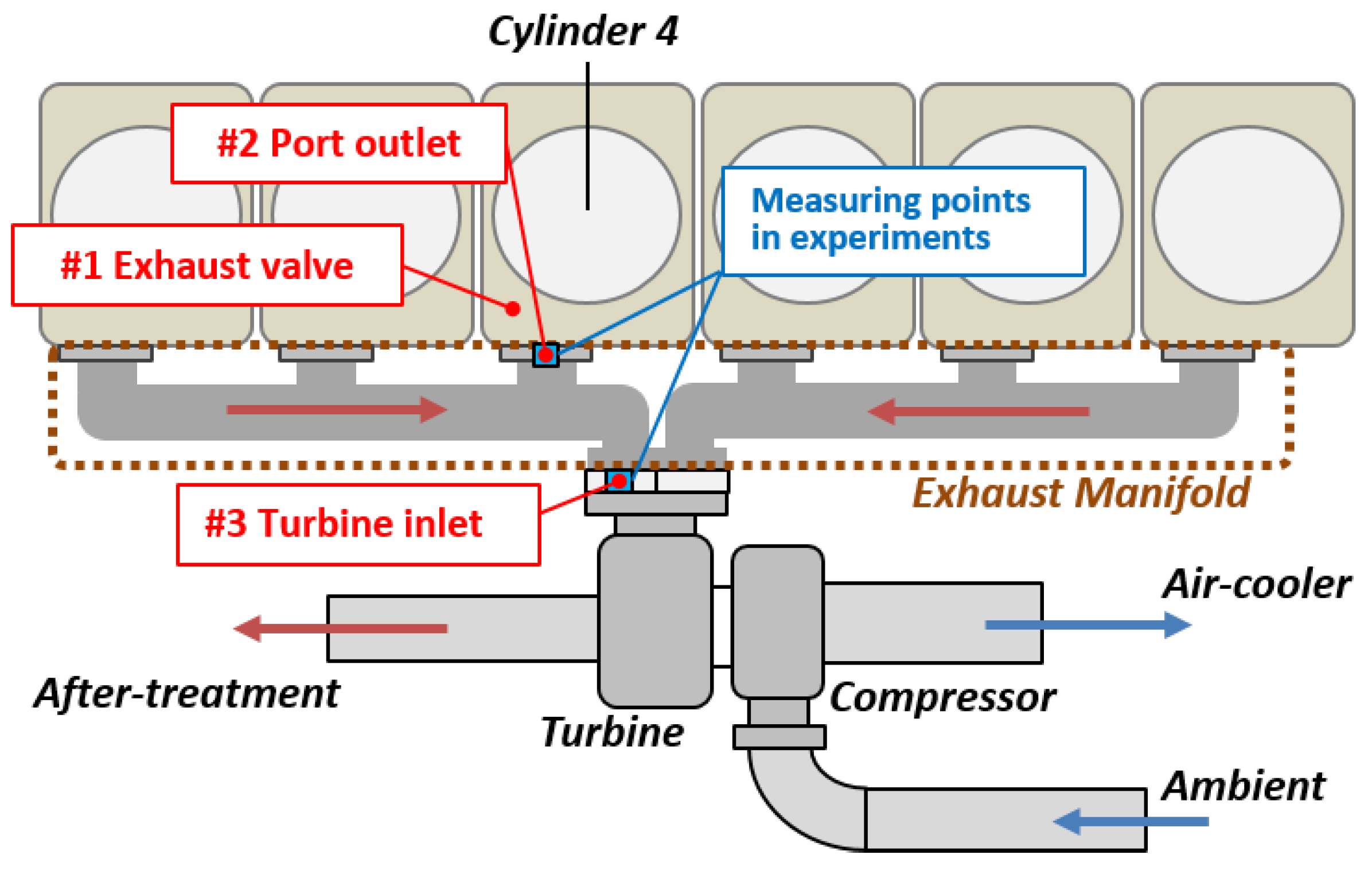
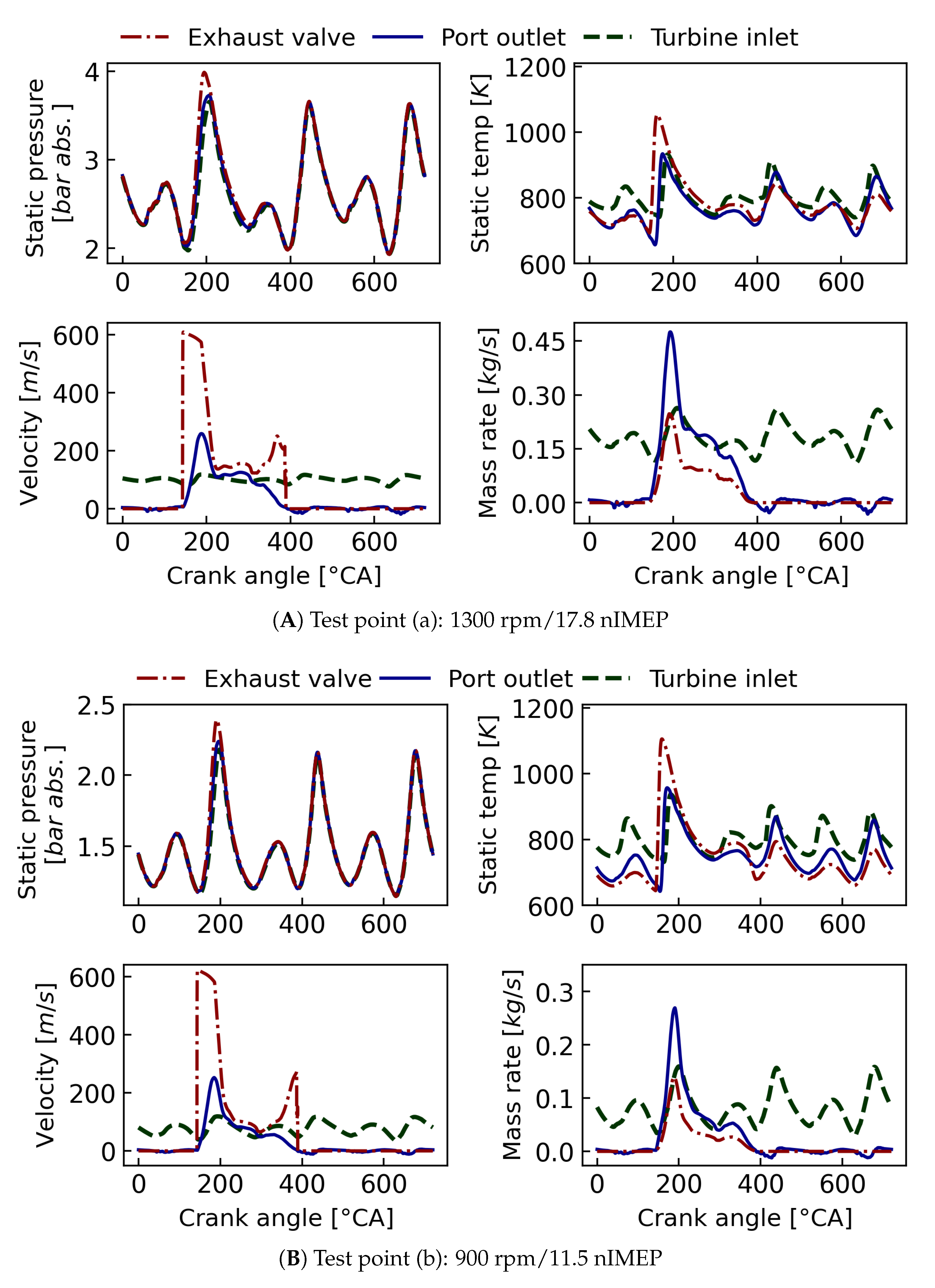
The engine system employed to provide reference exhaust pulses in this study is a commercial heavy-duty diesel engine (see Table 1). A schematic of the engine exhaust system is illustrated in Figure 1. To investigate exhaust pulsation under different speed/load conditions, two test points were selected: (a) engine speed at 1300 rpm (revolutions per minute), nIMEP (net indicated mean effective pressure) at 17.8 bar; (b) speed at 900 rpm, nIMEP at 11.5 bar. Operating conditions at test points are listed in Table 2. The instantaneous exhaust flow was calculated through numerical simulations based on a calibrated engine model. The 1D engine model was built and validated against experimental data using the commercial software package GT-Suite. A simplified turbocharger model was adopted by using experimental data and the combustion apparent heat release rate of the simulation was imposed by the measured cylinder pressure data. The valve model used in this study was built in a previous study [40] where the flow discharge coefficients of the exhaust valve were measured in a steady flow bench by a thermal mass flowmeter.
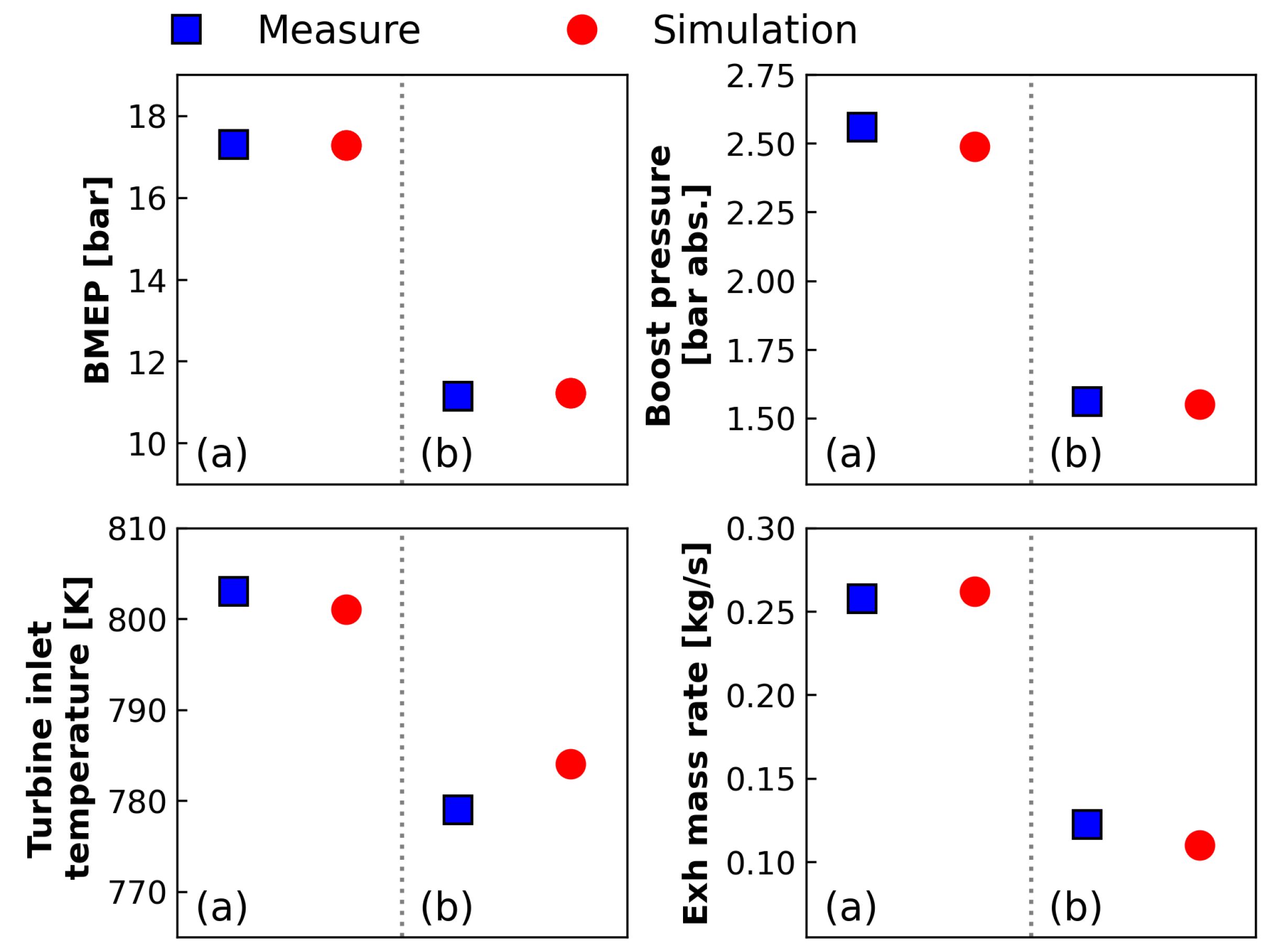
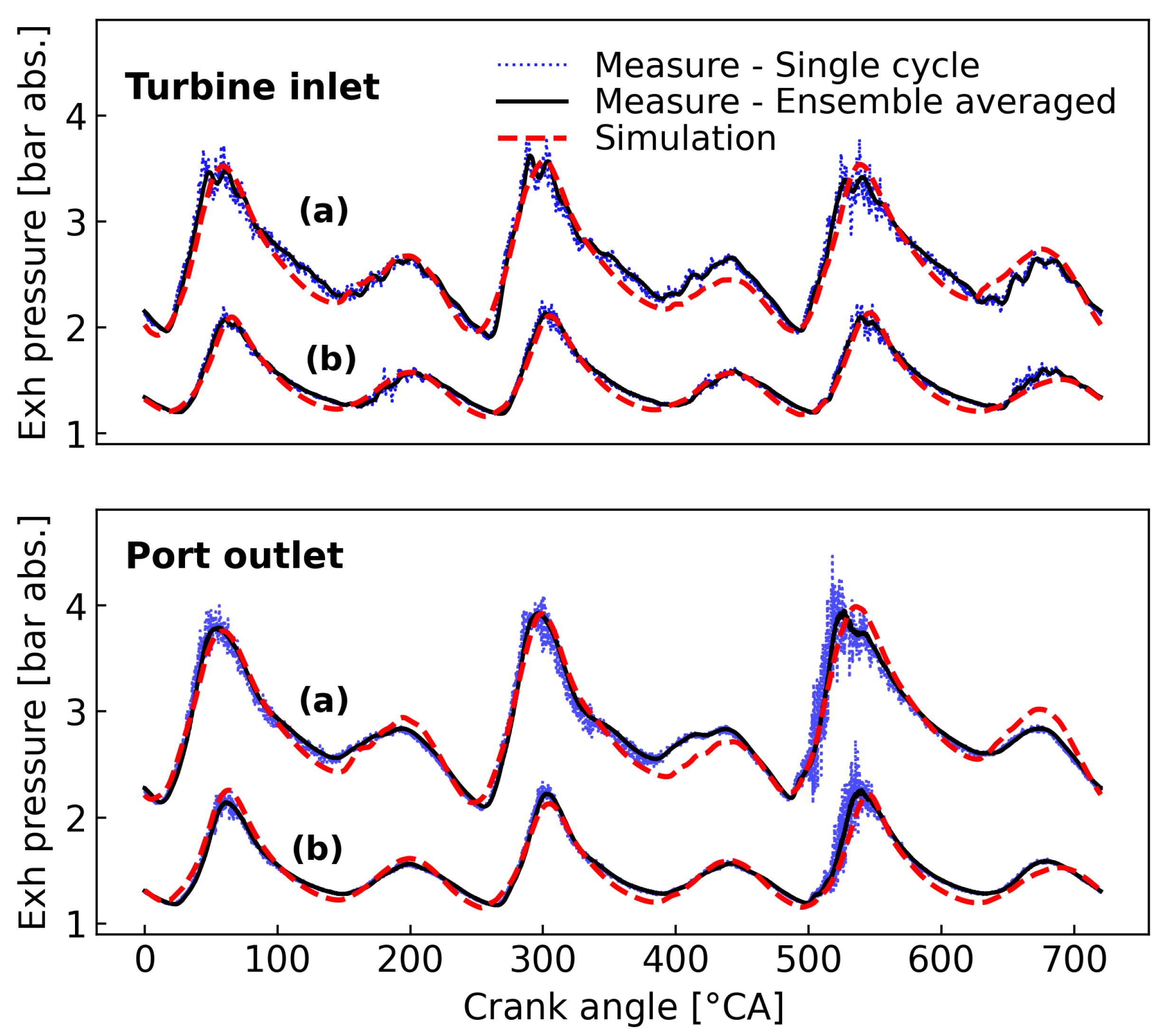
With special interest in the instantaneous exhaust flow parameters, measurement locations in the exhaust manifold were selected at the port outlet and the turbine inlet to acquire flow pressure and temperature. The fast exhaust pressure was sampled by water-cooled Kistler 4075A10 transducers and recorded at 200 kHz for 300 consecutive cycles, then downsampled and transferred to crank angle-based resolution with 0.1 crank angle (CA) interval. The flow temperature was measured by 3 mm K-type thermocouples, and only the mean value was taken from the thermocouple for temperature measurement due to its response limitation. The intake air flow rate was measured by an Annubar flow meter and the fuel injection per cycle was directly read from the engine control unit. An AVL GU21D pressure transducer was used to capture the cylinder pressure trace during the tests. Figure 2 shows the model validation regarding engine performances, where the maximum deviation is 3.6% for the exhaust mass rate at test point (b). In particular, Figure 3 compares the crank-angle-resolved exhaust pressure traces from measurement and simulation. The measurement data used in this study were obtained from a previous experiment in [5].
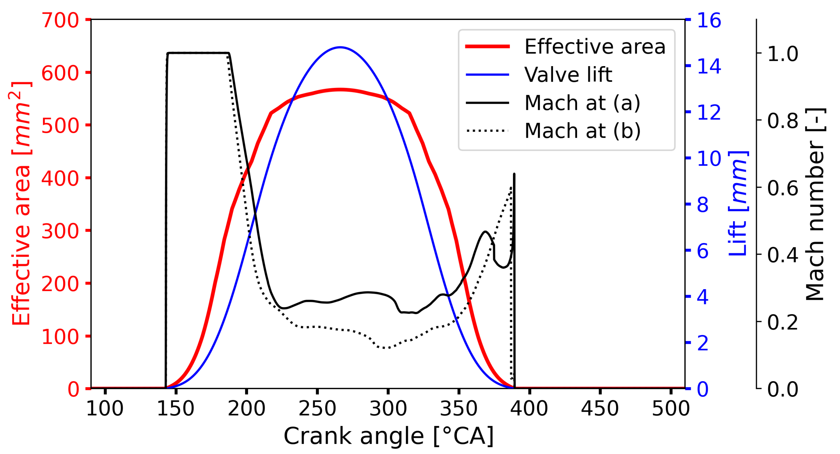
In this study, three measurement locations (as cross-sections) were selected in the exhaust system to analyze flow parameters, marked as red dots in Figure 1. The first location named by “exhaust valve” indicates the location at one of the twin ports close to the exhaust valve of cylinder 4. The “port outlet” location refers to the runner inlet where the exhaust gases enter the exhaust manifold. The third location, “turbine inlet”, was selected at an entry of the twin-entry radial turbine corresponding to the left-bank of manifold. These locations were chosen to illustrate the exhaust flow conditions from the opening of the exhaust valve to the entry of turbine. In particular, since the flow condition at the “exhaust valve” location is highly determined by valve motions based on the calibrated discharge coefficients [40], the effective area of exhaust valve and its correlation with the valve lift are shown in Figure 4. The flow velocity through the exhaust valve was chocked, i.e., , for roughly 50 CA after EVO for both test points. In addition, the effective area A of three measuring locations are listed in Table 3.
The flow pulsations at these measurement locations are illustrated in Appendix A. Note that, as shown in Figure A1, test point (b) had a higher peak temperature than (a) at the exhaust valve. This can be explained as, although the total mass of exhaust flow was smaller at (b), the lower engine speed can cause a stronger blowdown process by the slower valve opening. Additionally, the Mach 1 periods after EVO were similar for both test points as shown in Figure 4. Hence, the exhaust flow at test point (b) was mainly discharged at the blow-down process, which led to a higher temperature.
4. Results and Discussion
In this section, the impacts of exhaust flow parameters on the calculation of flow enthalpy and exergy are studied. Based on the exhaust flow condition of the tested engine, the enthalpy and exergy transport by engine exhaust pulsations were computed. Based on the crank-angle-resolved enthalpy and exergy, we then compared the potential errors induced by using cycle-averaged flow parameters. After a preliminary discussion of the effect of gas compositions on flow enthalpy and exergy computation, the sensitivities of time-varying flow parameters and their correlations with exhaust flow conditions were investigated. Apart from the theoretical analysis, the local and global SA methods were also applied to quantify the sensitivities.
4.1. Enthalpy and Exergy Pulsations
Based on the flow conditions of the exhaust pulsation (see Figure A1), the flow enthalpy and exergy were computed and analyzed on a unit-mass basis and mass flow rate form, respectively. These results are taken as the references in the next sections to study the impacts of flow parameters regarding the quantification of flow enthalpy and exergy of the exhaust pulses.
Figure 5 illustrates the specific enthalpy and exergy pulsation of the exhaust flows at different measurement locations. Naturally, the exhaust flow at test point (a) associated with a high operating load contains more enthalpy and exergy per unit mass. The specific enthalpy and exergy pulses have similar waveforms. Additionally, the specific enthalpy is always higher than the corresponding exergy, since the exergy can be taken as the useful part of enthalpy based on the second law [13]. In general, the enthalpy and exergy intensity are diminished along the exhaust path. For the pulsation generated during EVO to EVC, its enthalpy and exergy are reduced by the expansion and cooling process from the exhaust valve to the port outlet. After the exhaust enters the manifold and interacts with the other two pulses, the flow condition in the manifold has a limited effect on reducing the specific enthalpy and exergy.
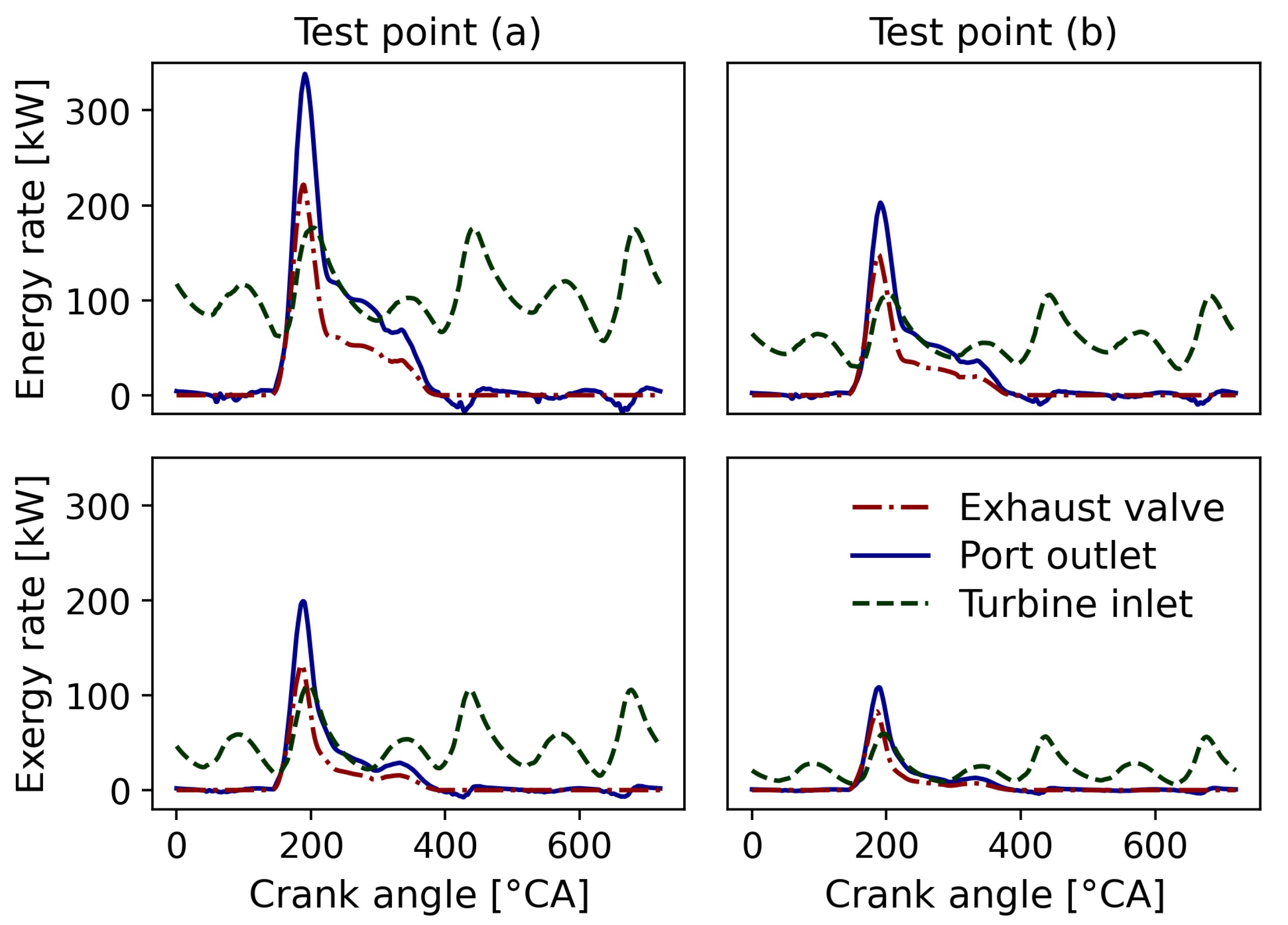
The magnitudes of enthalpy and exergy rates (in Figure 6) scale with the load of the tested points, the waveforms of enthalpy and exergy rates at the same test points differ across measurement locations. As the outflows of two exhaust valves with the same phase merge inside the port, the strongest enthalpy and exergy pluses appear at the port outlet. However, the expansion effect of the exhaust manifold is obvious where the peaks of enthalpy and exergy rates at the turbine inlet are reduced by half. As the turbine inlet gathers exhaust pulses from three cylinders in the left-bank of manifold, the total enthalpy and exergy rates at the turbine inlet are three times their values at the port outlet.
4.2. Cycle-Averaged Enthalpy and Exergy
Based on the enthalpy and exergy of instantaneous exhaust flows discussed above, this section presents the cycle-averaged results of flow enthalpy and exergy. The cycle-averaged flow quantity denotes the mean-value of pulses over one engine cycle by:
The cycle-averaged flow quantities of enthalpy and exergy are listed in Table 4. Meanwhile, the “error” column in Table 4 is presented to compare the cycle-averaged flow quantity with the result calculated by the mean value of the each flow parameter (i.e., by using , , and ).
It was found that the specific enthalpy and exergy transport by the exhaust flow decreases along the flow path. In contrast, the cycle-averaged enthalpy and exergy rates keep increasing as the exhaust flows assimilate.
In addition, denote the flow quantities based on the mean values of flow parameters (representative of “slow measurement”). As a result, from the measurement-orientated perspective, “error” here indicates the necessity of using fast flow parameters for engine exhaust studies. Confirming the conclusion in [20], the flow enthalpy and exergy calculated by using the mean of flow parameters are less than the results by using flow parameters having crank angle resolution. In particular, for the specific enthalpy, the “slow measurement” can give results with a maximum 6% error at the exhaust valve. However, significant errors can be observed in the case of enthalpy and exergy rates. For instance, at test point (b), there is an 8.4% error for exergy rate at the turbine inlet, where the flow condition is relatively stable, and for the measurement locations close to the exhaust valve, the error is significant, implying the requirement for fast flow parameter resolution.
4.3. Effect of Exhaust Gas Composition
Besides the time-varying flow parameters, the flow energy calculations in Equations (1)–(3) also depend on the gas composition of exhaust flow. Therefore, before the analyses of time-varying flow parameters, the effect of exhaust gas composition is discussed in this section. Differently from flow parameters (e.g., T, p, and u) that change with the propagation of exhaust pulses, the gas composition of engine exhaust is determined by the fuel–air ratio of the combustion process; meanwhile, the molar concentration of each gas component is constant during one engine cycle. In this study, the fuel–air equivalence ratio, , was introduced to calculate the gas composition of exhaust [34]. The combustion chemical calculations were conducted in a chemical kinetics Python library, Cantera [41], by using n-dodecane as the diesel surrogate with Polimi reduced chemical mechanism [42]. The exhaust molar concentrations of test points are listed in Table 5. Additionally, the gas composition of fresh air (i.e., = 0) and burnt gases of stoichiometric combustion (i.e., = 1) are included.
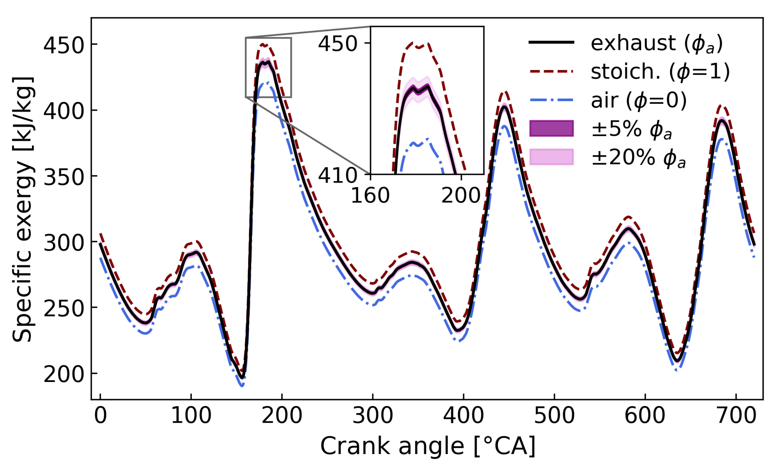
The effect of exhaust gas composition was examined by sweeping , while flow parameters of the exhaust remained unchanged. As an example, the result for specific exergy at the port outlet for test point (a) is shown in Figure 7. Note that the sweep of was intended to change the flow enthalpy and exergy calculations based on the exhaust gas composition, while the engine in-cylinder performance remains unchanged. The local SA was applied by varying 5% and 20% of . It shows that the difference caused by 5% sweeping was not significant for both specific and mass flow rate based flow enthalpy and exergy. For instance, in terms of specific energy quantities, the maximum absolute percentage error (MAPE) caused by the 20% sweeping was only 1.25% which occurred at the port outlet, test point (a) for exergy. MAPE for enthalpy and exergy rates was less than 0.01% (exhaust valve, test point (a) for exergy). Hence, although gas composition regarding the extreme cases (e.g., differences between air and the burnt gas from stoichiometric mixtures) can affect the flow enthalpy and exergy calculation, the local SA shows the impact of the variation in fuel–air equivalence ratio is negligible.
4.4. Analytical Solutions for the Sensitivity to Flow Parameters
In this section, the sensitivity to time-varying flow parameters is theoretically evaluated by a gradient based method. The analytical solutions here examine the effects of each flow parameter for computing the specific and mass flux based flow enthalpy and exergy, respectively. Instead of the mass flow rate based quantities, the mass flux based and were used to remove interference from different flow areas of different cross sections. In order to discuss the analytical solutions under the engine context, the ranges of flow parameters were taken from the exhaust flow conditions at the discussed test points. Moreover, because of the low sensitivity to the gas composition shown in the previous section, parameters such as coefficients of heat capacity and gas constant were taken from the exhaust condition of the engine at test point (a).
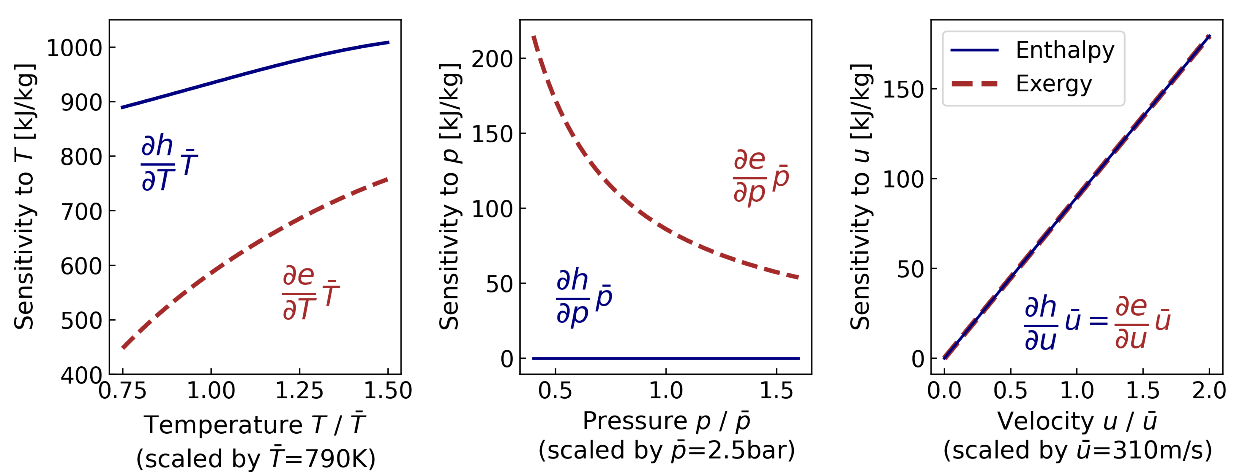
For specific enthalpy and exergy, the sensitivities of flow parameters were computed by taking the derivatives of Equations (1) and (3) with respect to temperature, pressure, and velocity. Results of the gradient-based method are shown in Figure 8, and the derivations of analytical solutions are presented in Appendix B. Since the derivative terms of flow specific enthalpy and exergy are independent of other flow parameters, the sensitivities discussed here are only determined by their corresponding flow parameters.
To compare the sensitivity among flow parameters, the derivatives and ranges of variables were normalized by the mean values of the exhaust parameters. Such a comparison shows that temperature is the most significant for assessing both specific enthalpy and exergy. The dominance of temperature was found for the evaluation of specific enthalpy. The significance of temperature for exergy is relatively lower, as not all of the energy is available to be transferred into work from the second law perspective. In the view of exergy analysis, the heat-related energy needs to be converted based on the Carnot efficiency. This indicates that the working fluid with higher temperatures has better energy quality associated with the potential to be transferred into work. Therefore, as the temperature increases, the increase of exergy sensitivity to temperature is more obvious than enthalpy. On the other hand, for the flow pressure p, the impact on flow specific exergy decreases at the high-pressure range; and for specific enthalpy, it does not affect it, since the pressure term is not included in the computation of specific enthalpy (1). For the flow velocity v, a comparable effect is noticed on enthalpy and exergy. This can be attributed to the kinetic energy (represented by flow velocity), which can be considered as the highest quality energy from the view of exergy analysis.
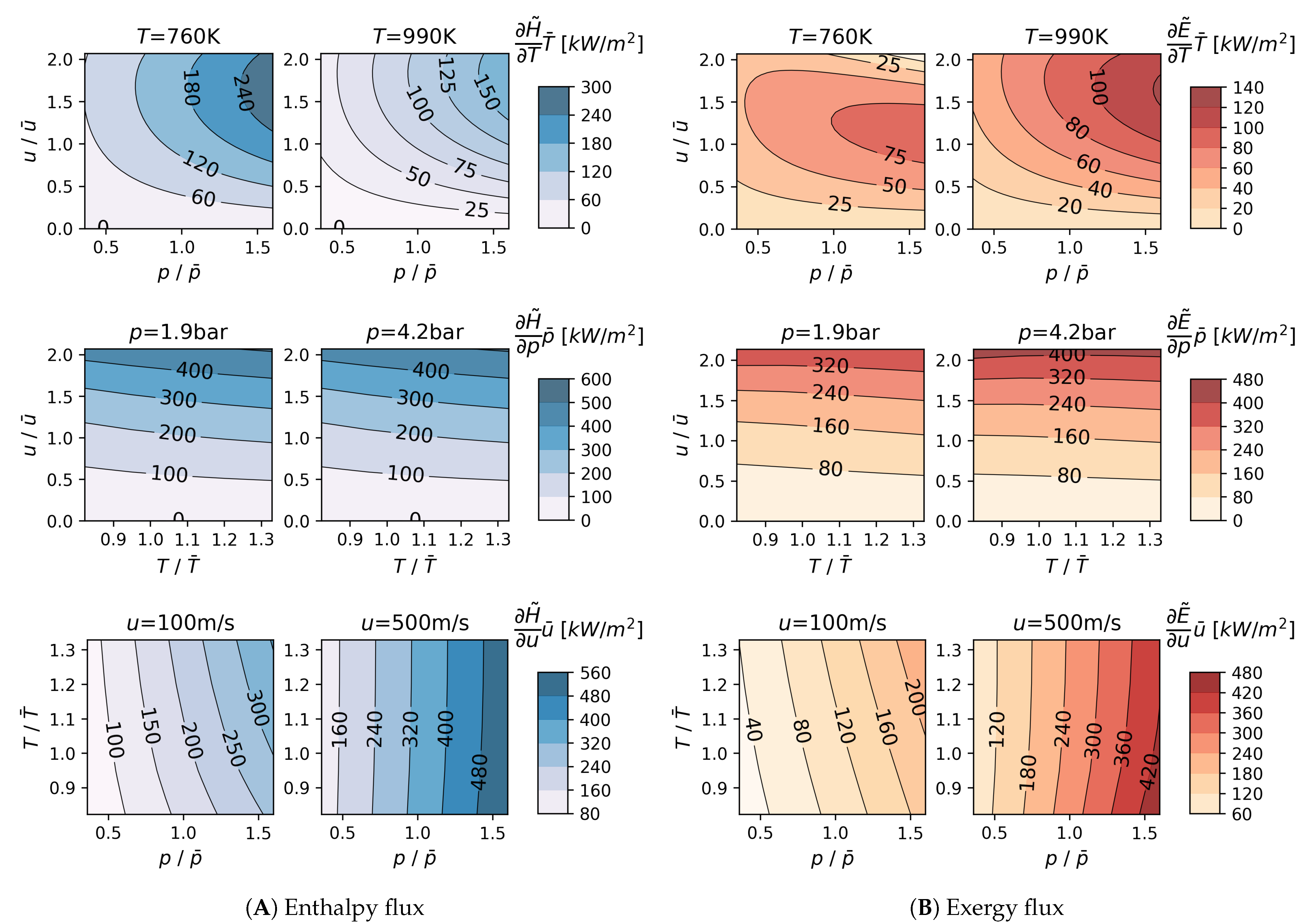
For the mass-flux-based enthalpy and exergy , the gradient-based sensitivities turned out to be more complex due to the interactions of other flow parameters. In an attempt to discuss the sensitivity of each parameter, results are demonstrated as contour plots in Figure 9. The analysis was conducted in two steps: (1) fixing the values of target parameters with selected low and high values, marked on the top of each contour plot; (2) sweeping and normalizing the ranges of the remaining parameters based on the same exhaust flow conditions used in Figure 8. Several characteristics can be found in these contour plots. In general, exergy rate is less sensitive to the changes in flow parameters than enthalpy rate due to the smaller magnitudes of flow exergy. The importance of pressure and velocity is increased compared to the previous case of flow specific h and e. In contrast, the sensitivity to temperature for flow enthalpy and exergy becomes the smallest, and the effect only appears when the pressure and velocity are above the mean values. In other words, temperature primarily affects the peak of flow enthalpy and exergy pulsations. The temperature sensitivity is more considerable for enthalpy flux at low-temperature conditions, but it shows an opposing trend for exergy. Additionally, the effect of flow velocity on mass flux quantities increases significantly in the high-velocity case, while the pressure sensitivity is also mainly affected by the flow velocity.
In summary, the analytical solution shows that the sensitivity of flow parameters are all monotonic and independent with other parameters for the specific-based enthalpy and exergy. The importance of temperature is dominant across the range of engine exhaust gases. However, for the mass flux based case, the flow pressure and velocity appear to be the most significant.
4.5. Local Sensitivity
Since the flow parameters are time-varying, their effects on the quantification of enthalpy and exergy pulsation are still dependent on the exhaust flow conditions. To investigate these impacts regarding the waveform of exhaust pulses, local sensitivity analysis (local SA) was applied by sweeping 5% across flow parameters to observe the resulting variations in flow enthalpy and exergy. Additionally, the cycle-averaged values of parameters (i.e., , , and ) were used to separately simulate the “slow measurement” on corresponding flow parameters. The difference between using cycle-averaged value and the instantaneous flow parameters indicates where the “fast measurement” is required to capture the pulsation of flow enthalpy and exergy. The measurement purpose also drove local SA to evaluate errors caused by inaccurate or slow response measurement. Furthermore, maximum absolute percentage errors (MAPE) were adopted to quantify the largest differences associated with such measurement uncertainties of flow parameters.
Results of local SA on specific enthalpy and exergy at test point (a) are depicted in Figure 10A for the exhaust valve, and Figure 10B for turbine inlet. The left column of each subplot is for enthalpy, and the exergy is on the right. By comparing the deviation by sweeping flow parameters, it was found that the sensitivity of exhaust pulses changes with flow waveform. Besides the dominant effect of temperature, the uncertainty brought by pressure becomes significant at the non-peak part of pulse (i.e., low-p area). Meanwhile, the velocity sensitivity mainly appears at the exhaust valve after EVO.
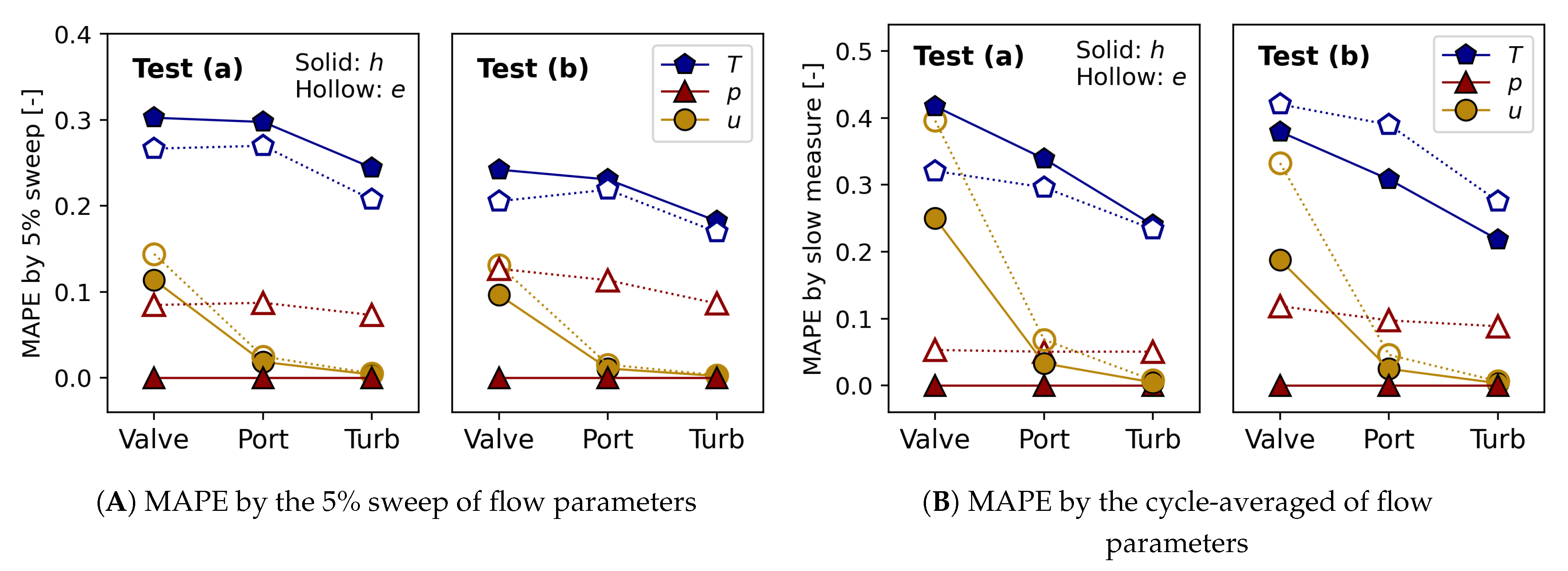
Such local SA results are also in agreement with the conclusions from theoretical solutions discussed in Section 4.4. Moreover, MAPE in Figure 11A quantifies the maximum deviation of specific enthalpy and exergy caused by 5% variations in flow parameters. For the specific flow energy quantities of exhaust pulses, the high sensitivity of temperature implies that the thermal energy contributed by flow temperature is the major portion of specific enthalpy and exergy. It was found that a 5% sweep over the temperature pulse lead to maximum deviations of 31% and 27% when resolving the crank angle-based specific enthalpy and specific exergy, respectively. Although the sensitivity of flow velocity on specific enthalpy and exergy are comparable as discussed in Section 4.4, the MAPE of velocity on exergy is due to the lower magnitude of the exergy pulse compared to the enthalpy.
In addition, the comparison between using “fast” (instantaneous) and “slow” (cycle-averaged) flow parameters shows that in order to capture the pulses of specific enthalpy and exergy, the crank-angle-resolved temperature is needed. Meanwhile, resolving the velocity pulse at the exhaust valve becomes more critical due to its large fluctuation in this location. Furthermore, the similar trends of MAPE in Figure 11B indicates that instead of engine operating conditions, the demand for using instantaneous flow parameters mainly depends on the measuring location in the current assessment.
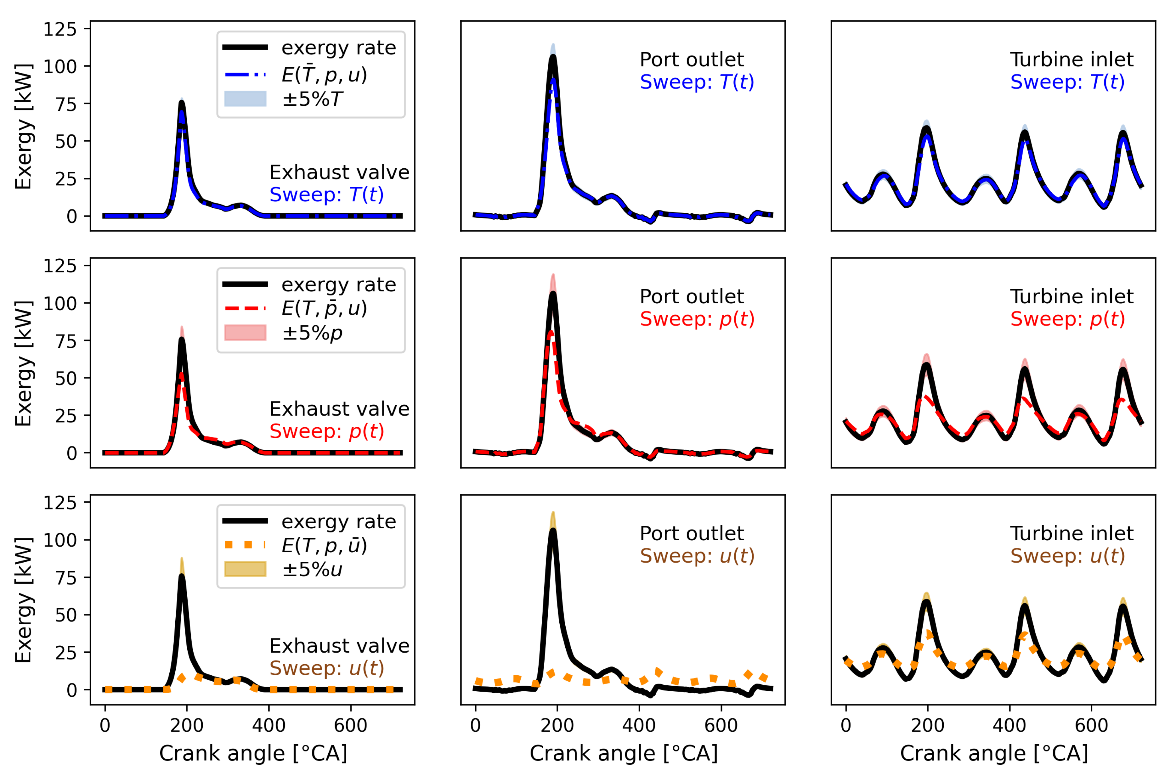
Since the results of local SA on enthalpy and exergy rates are similar, the exergy rate at test point (b) was chosen to present the sensitivity at three measuring locations in Figure 12. According to the local SA results of the 5% sweeps of instantaneous flow parameters, the influence of temperature variation decreased considerably, and deviations due to the variations in flow pressure and velocity are noticeable. These observations support the conclusion from the theoretical analysis in Section 4.4. Moreover, compared to the sensitivity of specific flow energy quantities, a lower deviation was caused by the 5% sweep for flow energy rates. The most sensible areas appear at the peaks of pulses where the flow parameters are also at their peak values. On the other hand, the comparison between using “fast” and “slow” flow parameters indicates the significance of using the instantaneous velocity. Besides, the "fast" flow pressure is also necessary for quantifying the flow exergy at the turbine inlet.
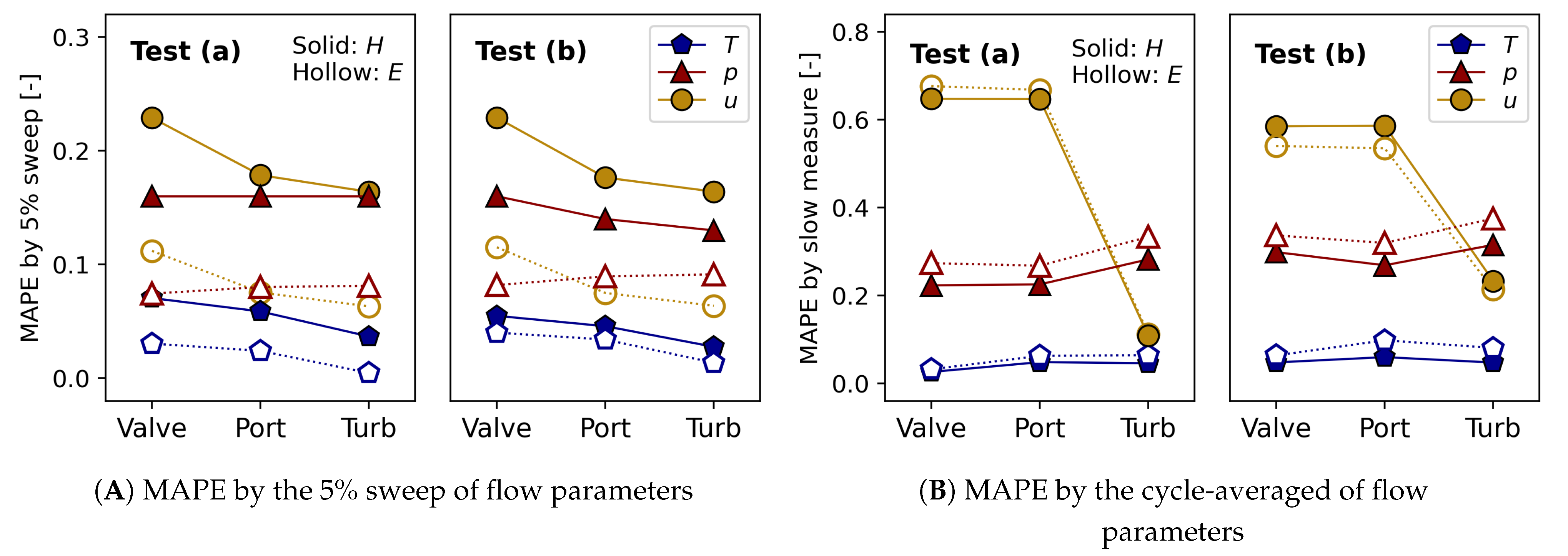
MAPE of enthalpy and exergy rates quantification are shown in Figure 13. Regarding the variation caused by flow parameter sweeping, velocity is higher than pressure for exergy rate while they are similar for enthalpy. Note that MAPE by sweeping flow parameter is higher for enthalpy rates, indicating that the exergy rate calculation is more robust to the variations in instantaneous flow parameters. Flow velocity is the most significant parameter requiring high resolution, with a maximum deviation of 23% for the enthalpy rate and 12% for the exergy rate over a 5% sweep of the flow velocity pulse, as shown in Figure 13A. Furthermore, the MAPE by “slow” flow parameters shows that the lack of instantaneous flow velocity may lead to significant calculation errors of instantaneous enthalpy and exergy rates at measuring locations where the fluctuations of pulses are intense, such as exhaust valve and port outlet. Moreover, the instantaneous pressure becomes most important for the enthalpy and exergy evaluations at the turbine inlet.
4.6. Global Sensitivity
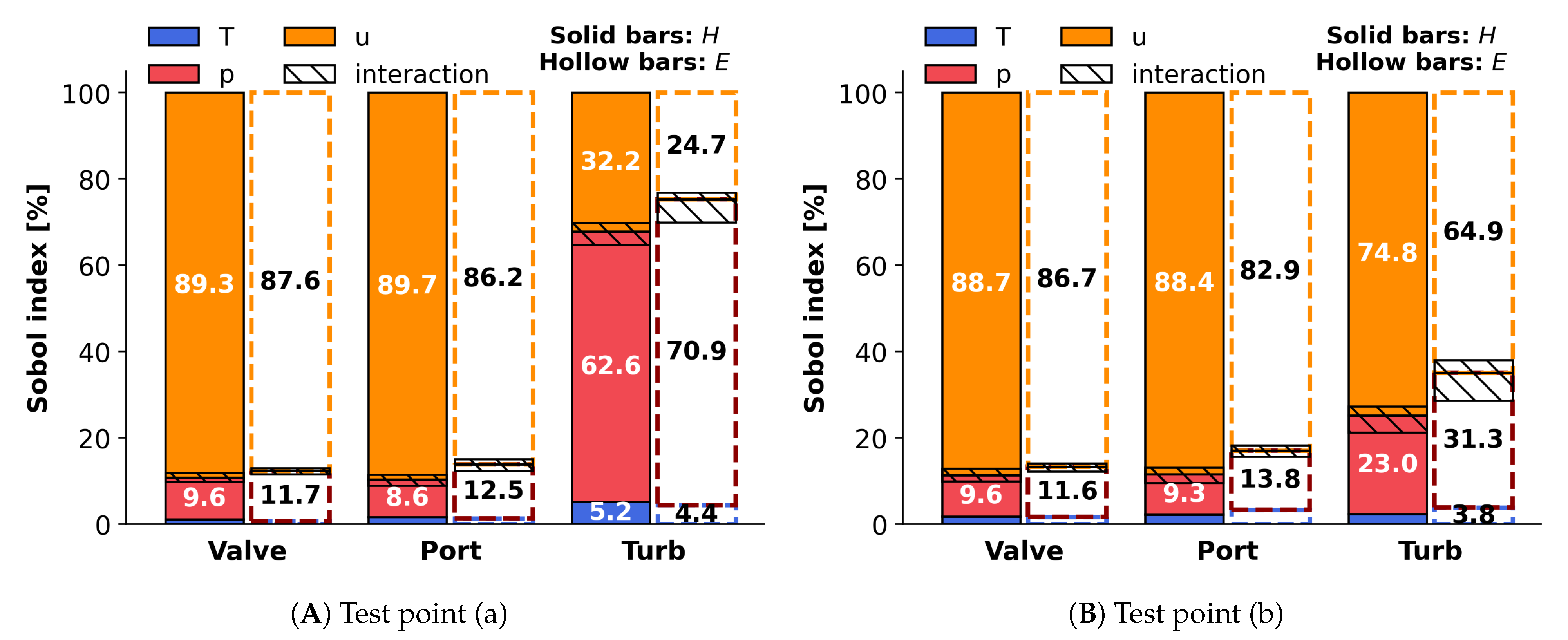
In this section, a variance-based analysis prioritizes the impacts of input variables on the computation of flow enthalpy and exergy. In global SA, Sobol indices represent the relative significance of each flow parameter regarding the flow condition at different measuring locations and test points. Moreover, the interactions among flow parameters are quantified by the differences between Sobol total and main effect indices (i.e., ). Note that the Sobol indices in Figure 14 and Figure 15 refer to the Sobol total effect indices, and the shaded area denotes the flow parameter interaction.
Figure 14 shows the significance of exhaust flow parameters for specific enthalpy and exergy in the exhaust pulses. For specific enthalpy, it clearly shows the dominant significance of temperature, especially for the locations of port outlet to turbine inlet where the fluctuations of the flow parameters are relatively minimized. Similarly, for specific exergy, the maximum calculation uncertainty can still be attributed to temperature. The impact of flow velocity increases at the exhaust valve, and pressure shows more significance at the port outlet and the turbine inlet. Moreover, the sensitivities of p and u at test point (a) are higher than at (b) due to the intense exhaust dynamics at the high engine load and speed. As there was no interaction among flow parameters here, they were independent for assessing specific enthalpy and exergy.
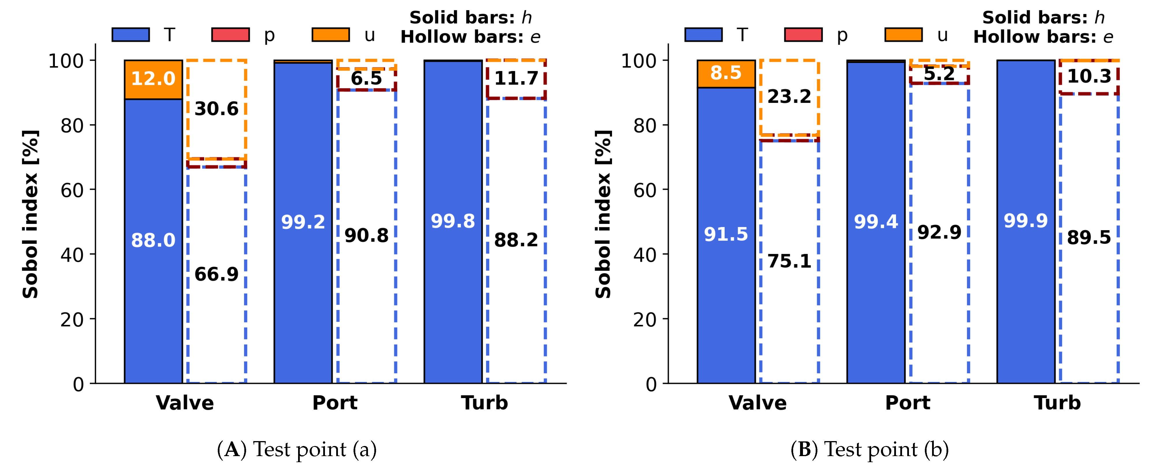
In Figure 15, Sobol indices for computing enthalpy and exergy rates in the exhaust pulses show the significance of using crank angle-based flow velocity and pressure. As shown in previous sections, the significance of flow temperature reduced to less than 5.2%. The importance of flow pressure rose at the turbine inlet, especially for test point (a) where the change of flow p increased and u became stable due to the wider mass flow range. The shadowed areas specifically denote the interactions among flow parameters in the assessments of exhaust enthalpy and exergy rates. It can be found that the interaction mainly happened between flow u and p, which means their sensitivities rely on each other, wherein u has more influence on p. The largest interaction between u and p occurred at the turbine inlet. At test point (b), the interaction with p caused 3.5% significance of u, and this interaction counted for 8.7% of the significance of p.
5. Conclusions
In this study, the impacts of flow parameters on the enthalpy and exergy of pre-turbine engine exhaust pulsations were evaluated. Referring to the unsteady exhaust conditions of a heavy-duty diesel engine, the sensitivities of specific and mass flow rate based flow enthalpy and exergy were respectively quantified in terms of flow parameters (i.e., T, p, and u). Firstly, the exhaust gas enthalpy and exergy pulsation at selected measuring locations were presented. This, followed by an analytical solution, illustrated the trends of flow parameter sensitivities concerning different exhaust flow conditions. Additionally, according to the results of local and global sensitivity analysis, the effects of flow parameters on the energy assessment of exhaust gas pulses were further discussed.
- Based on the exhaust flow conditions at different locations, it was found that the degrees of specific enthalpy and exergy fluctuation decreased from the exhaust valve to the turbine inlet. This can be explained by the reduced fluctuation of the respective flow parameters across the different locations due to expansion and pulse interaction effects. Moreover, the waveforms of flow enthalpy and exergy rates are determined by the instantaneous mass flow rate.
- For evaluating the cycle-averaged flow enthalpy and exergy using mean values of the flow parameters (representative of “slow measurements”), the need for high resolution flow parameters was indicated for accurate computations of the cycle-averaged enthalpy and exergy rates irrespective of the physical location and with greater error reduction potential towards stronger pulsating flow (from turbine inlet towards the exhaust valve). However, the errors in specific enthalpy and exergy computation appear to have less significance for high resolution flow parameters, especially in the turbine inlet conditions of the analyzed cases.
- The variations in exhaust gas composition had negligible impacts on the flow enthalpy and exergy quantification.
- The analytical solution revealed that flow temperature fluctuations are the most significant for computing specific enthalpy and exergy. However, pressure and velocity fluctuations are the primary factors for assessing the total enthalpy and exergy rates.
- For specific flow enthalpy and exergy, the effect of flow pressure mainly occurred at the low-p area of the pulse, whereas the influence of flow velocity was concentrated on the high-u region. As previously mentioned, temperature’s sensitivity was observable through the entirety of the exhaust pulse. Unlike the specific flow enthalpy and exergy, for the enthalpy and exergy rates, the deviations caused by the sweep of 5% flow parameter were minor, and the observed sensitivity mainly appeared at the peaks of exhaust pulses where the flow parameters were also at their peak values.
- As a representation of the responses of “slow” flow measurements, the cycle-averaged flow parameters were used in the local SA to illustrate the deviations of pulse shapes in terms of the flow enthalpy and exergy. A comparison of cycle-resolved and cycle-averaged flow parameters showed that high resolution temperature and velocity are required to accurately capture the specific enthalpy and exergy. However, when evaluating the total enthalpy and exergy rates, a high resolution of velocity is the most important, especially at locations before the exhaust manifold, and high resolution of the pressure pulse becomes necessary at the turbine inlet.
- Sobol indices in the global SA show that temperature contributed at least 88% sensitivity to specific enthalpy and 66.9% to specific exergy. Moreover, the specific exergy sensitivity to flow velocity was relatively larger than that of the the specific enthalpy. On the other hand, for enthalpy and exergy rates, the sensitivity of flow velocity was most significant for most cases. In addition, at the turbine inlet, the significance of pressure increased to 62% for enthalpy rate and 70% for exergy rate.
Author Contributions
Conceptualization, A.C., B.H. and V.V.; methodology, B.H. and V.V.; software, B.H.; validation, B.H., V.V. and A.C.; formal analysis, B.H.; investigation, B.H., V.V. and A.C.; writing—original draft preparation, B.H.; writing—review and editing, B.H., V.V. and A.C.; visualization, B.H.; supervision, A.C.; project administration, A.C. All authors have read and agreed to the published version of the manuscript.
Funding
This research was funded by the Swedish Energy Agency and the Competence Center for Gas Exchange (CCGEx).
Institutional Review Board Statement
Not applicable.
Informed Consent Statement
Not applicable.
Data Availability Statement
Not applicable.
Acknowledgments
The authors would like to thank Ted Holmberg from Scania CV AB for his kind support with the GT-Power model and engine experiments. The support from Anders Christiansen Erlandsson from Technical University of Denmark at the early stage of this work is acknowledged. We also greatly appreciate Yushi Murai, David Leffler, and Arun Prasath K. for their discussions about ideas. The Swedish Energy Agency, the Competence Center for Gas Exchange (CCGEx) and its partners are acknowledged for funding this study.
Conflicts of Interest
The authors declare no conflict of interest.
Nomenclatures
| Abbreviations | |
| ICE | Internal combustion engine |
| nIMEP | Net indicated mean effective pressure |
| BMEP | Brake mean effective pressure |
| CA | Crank angle |
| IVO | Intake valve opening |
| IVC | Intake valve closing |
| EVO | Exhaust valve opening |
| EVC | Exhaust valve closing |
| BBDC | Before bottom dead centre |
| ATDC | After top dead centre |
| SA | Sensitivity analysis |
| MAPE | Maximum absolute percentage error |
| Notations | |
| H | Enthalpy rate [kW] |
| E | Exergy rate [kW] |
| h | Specific stagnation enthalpy [kJ/kg] |
| e | Specific exergy [kJ/kg] |
| s | Specific entropy [] |
| Mass flow rate [kg/s] | |
| p | Static pressure [bar abs.] |
| T | Static temperature [K] |
| u | Flow velocity [m/s] |
| Specific heat capacity [] | |
| Specific gas constant of gaseous mixture [] | |
| Flow density [] | |
| Heat capacity ratio [-] | |
| Coefficients of NASA polynomial | |
| M | Mach number [-] |
| Crank angle [] | |
| Mass flux based enthalpy rate [] | |
| Mass flux based exergy rate [] | |
| A | Effective cross-sectional flow area [] |
| Fuel–air equivalence ratio [-] | |
| Ambient pressure [bar abs.] | |
| Ambient temperature [K] | |
| Sobol main effect index for the ith component [%] | |
| Sobol total effect index for ith component [%] | |
| Variance of a variable | |
| Conditional expected value with a given x | |
| Input and output variables for sensitivity analysis | |
Appendix A. Exhaust Flow Parameters at Three Measurement Locations
Flow conditions of exhaust pulsations at measurement locations are computed using the calibrated GT-Power engine model. The flow parameters are illustrated in Figure A1, while the mass flow rates are calculated based on Equation (6).
Figure A1.
Exhaust flow conditions at three measurement locations operating at test points.

Appendix B. Derivation of Analytical Solutions
In this section, we present the mathematical derivations for the analytical solutions for the sensitivities with respect to each individual flow parameter (i.e., T, p, and u). As explained in Section 4.4, the solutions of such sensitivity can be interpreted as partial derivatives of the specific-based and mass-flux-based flow enthalpy and exergy shown in Section 2.1. In addition, the pressure and temperature at the dead state (i.e., ambient condition) are denoted by and . First, for the specific-based energy in (1), the partial derivatives with respect to flow parameters are
Additionally, for the specific-based exergy in (3), the partial derivatives with respect to flow parameters are
However, for the mass-flux-based case, the interaction from other flow parameters can be found. Based on (4) and (6), the partial derivatives of mass-flux-based energy are
Similarly, the partial derivatives of mass-flux-based exergy can be given by using (5) and (6) as
where the heat capacity can be approximated by a NASA polynomial function of temperature, as shown in Equation (2). Therefore, its relevant integrations used in derivations above are also polynomial functions of temperature:
Note that the gas constant and heat capacity coefficients are determined by exhaust gas composition. In this study, for test points (a) and (b), these parameters are computed by combustion reactions based on the fuel–air equivalence ratio . The result of gas-composition-based parameters for exhaust flows is listed in Table A1.

Table A1.
Fuel–air equivalence ratio , mass-basis gas constant and specific heat capacity coefficients for exhaust gases at test points (a) and (b). The unit of and is: [J · kg· K].
Table A1.
Fuel–air equivalence ratio , mass-basis gas constant and specific heat capacity coefficients for exhaust gases at test points (a) and (b). The unit of and is: [J · kg· K].
| (a) | 0.532 | 289.191 | 3.511 | 0.065 | 0.968 | −0.132 | −0.191 |
| (b) | 0.581 | 289.280 | 3.505 | 0.142 | 0.858 | −0.504 | −0.214 |
References
- Conway, G.; Joshi, A.; Leach, F.; García, A.; Senecal, P.K. A review of current and future powertrain technologies and trends in 2020. Transp. Eng. 2021, 5, 100080. [Google Scholar] [CrossRef]
- Primus, R.J. A second law approach to exhaust system optimization. In SAE International Congress and Exposition; SAE International: Warrendale, PA, USA, 1984. [Google Scholar] [CrossRef]
- Hatami, M.; Boot, M.; Ganji, D.; Gorji-Bandpy, M. Comparative study of different exhaust heat exchangers effect on the performance and exergy analysis of a diesel engine. Appl. Therm. Eng. 2015, 90, 23–37. [Google Scholar] [CrossRef]
- Copeland, C.D.; Martinez-Botas, R.; Seiler, M. Comparison between steady and unsteady double-entry turbine performance using the quasi-steady assumption. J. Turbomach. 2011, 133, 031001. [Google Scholar] [CrossRef]
- Holmberg, T.; Cronhjort, A.; Stenlaas, O. Pressure Amplitude Influence on Pulsating Exhaust Flow Energy Utilization. In Proceedings of the SAE 2018 World Congress, Warrendale, PA, USA, 10–12 April 2018; SAE International: Warrendale, PA, USA, 2018. [Google Scholar] [CrossRef]
- Lim, S.M.; Dahlkild, A.; Mihaescu, M. Influence of Upstream Exhaust Manifold on Pulsatile Turbocharger Turbine Performance. J. Eng. Gas Turbines Power 2019, 141, 061010. [Google Scholar] [CrossRef]
- Lim, S.M.; Dahlkild, A.; Mihaescu, M. Aerothermodynamics and exergy analysis in radial turbine with heat transfer. J. Turbomach. 2018, 140, 091007. [Google Scholar] [CrossRef]
- Luján, J.M.; Serrano, J.R.; Piqueras, P.; Diesel, B. Turbine and exhaust ports thermal insulation impact on the engine efficiency and aftertreatment inlet temperature. Appl. Energy 2019, 240, 409–423. [Google Scholar] [CrossRef]
- Simonetti, M.; Caillol, C.; Higelin, P.; Dumand, C.; Revol, E. Experimental investigation and 1D analytical approach on convective heat transfers in engine exhaust-type turbulent pulsating flows. Appl. Therm. Eng. 2020, 165, 114548. [Google Scholar] [CrossRef]
- Yang, M.; Gu, Y.; Deng, K.; Yang, Z.; Liu, S. Influence of altitude on two-stage turbocharging system in a heavy-duty diesel engine based on analysis of available flow energy. Appl. Therm. Eng. 2018, 129, 12–21. [Google Scholar] [CrossRef]
- Zheng, Z.; Feng, H.; Mao, B.; Liu, H.; Yao, M. A theoretical and experimental study on the effects of parameters of two-stage turbocharging system on performance of a heavy-duty diesel engine. Appl. Therm. Eng. 2018, 129, 822–832. [Google Scholar] [CrossRef]
- Rakopoulos, C.D.; Giakoumis, E.G. Second-law analyses applied to internal combustion engines operation. Prog. Energy Combust. Sci. 2006, 32, 2–47. [Google Scholar] [CrossRef]
- Bejan, A.; Tsatsaronis, G.; Moran, M.J. Thermal Design and Optimization; John Wiley & Sons: Hoboken, NJ, USA, 1995. [Google Scholar]
- Wang, B.; Pamminger, M.; Wallner, T. Impact of fuel and engine operating conditions on efficiency of a heavy duty truck engine running compression ignition mode using energy and exergy analysis. Appl. Energy 2019, 254, 113645. [Google Scholar] [CrossRef]
- Mahabadipour, H.; Srinivasan, K.K.; Krishnan, S.R.; Subramanian, S.N. Crank angle-resolved exergy analysis of exhaust flows in a diesel engine from the perspective of exhaust waste energy recovery. Appl. Energy 2018, 216, 31–44. [Google Scholar] [CrossRef]
- Zhang, H.; Zhang, H.; Wang, Z. Effect on Vehicle Turbocharger Exhaust Gas Energy Utilization for the Performance of Centrifugal Compressors under Plateau Conditions. Energies 2017, 10, 2121. [Google Scholar] [CrossRef] [Green Version]
- Hong, B.; Mahendar, S.K.; Hyvönen, J.; Cronhjort, A.; Erlandsson, A.C. Quantification of Losses and Irreversibilities in a Marine Engine for Gas and Diesel Fuelled Operation Using an Exergy Analysis Approach. In Proceedings of the ASME 2000 Internal Combustion Engine Division Fall Technical Conference, Virtual, 4–6 November 2020. [Google Scholar] [CrossRef]
- Valencia, G.; Fontalvo, A.; Cárdenas, Y.; Duarte, J.; Isaza, C. Energy and Exergy Analysis of Different Exhaust Waste Heat Recovery Systems for Natural Gas Engine Based on ORC. Energies 2019, 12, 2378. [Google Scholar] [CrossRef] [Green Version]
- Mamalis, S.; Babajimopoulos, A.; Assanis, D.; Borgnakke, C. A modeling framework for second law analysis of low-temperature combustion engines. Int. J. Engine Res. 2014, 15, 641–653. [Google Scholar] [CrossRef]
- Chen, H.; Hakeem, I.; Martinez-Botas, R. Modelling of a turbocharger turbine under pulsating inlet conditions. Proc. Inst. Mech. Eng. A 1996, 210, 397–408. [Google Scholar] [CrossRef]
- Baines, N. Turbocharger turbine pulse flow performance and modeling-25 years on. In Proceedings of the 9th International Conference on Turbochargers and Turbocharging, IMechE, London, UK, 19–20 May 2010. [Google Scholar]
- Tagawa, M.; Ohta, Y. Two-thermocouple probe for fluctuating temperature measurement in combustion—Rational estimation of mean and fluctuating time constants. Combust. Flame 1997, 109, 549–560. [Google Scholar] [CrossRef]
- Kar, K.; Roberts, S.; Stone, R.; Oldfield, M.; French, B. Instantaneous Exhaust Temperature Measurements Using Thermocouple Compensation Techniques; SAE Technical Paper; SAE International: Warrendale, PA, USA, 2004. [Google Scholar] [CrossRef]
- Papaioannou, N.; Leach, F.; Davy, M. Improving the Uncertainty of Exhaust Gas Temperature Measurements in Internal Combustion Engines. J. Eng. Gas Turbines Power 2020, 142, 071007. [Google Scholar] [CrossRef]
- Benson, R.S.; Brundrett, G.W. Development of a resistance wire thermometer for measuring transient temperatures in exhaust systems of internal combustion engines. In Temperature—Its Measurement and Control in Science and Industry; Reinhold: New York, NY, USA, 1962; Volume 3, pp. 631–653. [Google Scholar]
- Venkataraman, V.; Murai, Y.; Liverts, M.; Örlü, R.; Fransson, J.H.M.; Stenlåås, O.; Cronhjort, A. Resistance Wire Thermometers for Temperature Pulse Measurements on Internal Combustion Engines. In Proceedings of the SMSI 2020 Conference-Sensor and Measurement Science International, Nuremberg, Germany, 22–25 June 2020. [Google Scholar]
- Mollenhauer, K. Measurement of Instantaneous Gas Temperatures for Determination of the Exhaust Gas Energy of a Supercharged Diesel Engine; SAE Technical Paper; SAE International: Warrendale, PA, USA, 1967. [Google Scholar]
- Zhao, H.; Ladommatos, N. Engine Combustion Instrumentation and Diagnostics; Society of Automotive Engineers: Warrendale, PA, USA, 2001; Volume 842. [Google Scholar]
- Ehrlich, D.A.; Lawless, P.B.; Fleeter, S. Particle Image Velocimetry Characterization of a Turbocharger Turbine Inlet Flow; Technical Report, SAE Technical Paper; SAE International: Warrendale, PA, USA, 1997. [Google Scholar]
- Ehrlich, D.A. Characterization of Unsteady on-Engine Turbocharger Turbine Performance. Ph.D. Thesis, Purdue University, West Lafayette, IN, USA, 1998. [Google Scholar]
- Lakshminarayanan, P.; Janakiraman, P.; Babu, M.G.; Murthy, B. Measurement of pulsating temperature and velocity in an internal combustion engine using an ultrasonic flowmeter. J. Phys. E Sci. Instrum. 1979, 12, 1053. [Google Scholar] [CrossRef]
- Avola, C.; Copeland, C.; Romagnoli, A.; Burke, R.; Dimitriou, P. Attempt to correlate simulations and measurements of turbine performance under pulsating flows for automotive turbochargers. Proc. Inst. Mech. Eng. D 2019, 233, 174–187. [Google Scholar] [CrossRef]
- Mahabadipour, H.; Partridge, K.R.; Jha, P.R.; Srinivasan, K.K.; Krishnan, S.R. Characterization of the Effect of Exhaust Back Pressure on Crank Angle-Resolved Exhaust Exergy in a Diesel Engine. J. Eng. Gas Turbines Power 2019, 141, 081016. [Google Scholar] [CrossRef]
- Heywood, J.B. Internal Combustion Engine Fundamentals; McGraw-Hill Series in Mechanical Engineering; McGraw-Hill Education: New York, NY, USA, 1989. [Google Scholar]
- Anderson, J.D. Modern Compressible Flow; McGraw-Hill Education: New York, NY, USA, 2003. [Google Scholar]
- Borgonovo, E.; Plischke, E. Sensitivity analysis: A review of recent advances. Eur. J. Oper. Res. 2016, 248, 869–887. [Google Scholar] [CrossRef]
- Saltelli, A.; Tarantola, S.; Campolongo, F.; Ratto, M. Sensitivity Analysis in Practice: A Guide to Assessing Scientific Models; Wiley Online Library: Hoboken, NJ, USA, 2004; Volume 1. [Google Scholar]
- Sobol’, I. Global sensitivity indices for nonlinear mathematical models and their Monte Carlo estimates. Math. Comput. Simul. 2001, 55, 271–280. [Google Scholar] [CrossRef]
- Herman, J.; Usher, W. SALib: An open-source Python library for sensitivity analysis. J. Open Source Softw. 2017, 2, 97. [Google Scholar] [CrossRef]
- Holmberg, T.; Cronhjort, A.; Stenlaas, O. Pressure Ratio Influence on Exhaust Valve Flow Coefficients. In Proceedings of the SAE 2017 World Congress, Detroit, MI, USA, 4–6 April 2017; SAE International: Warrendale, PA, USA, 2017. [Google Scholar] [CrossRef]
- Goodwin, D.G.; Speth, R.L.; Moffat, H.K.; Weber, B.W. Cantera: An Object-Oriented Software Toolkit for Chemical Kinetics, Thermodynamics, and Transport Processes; Version 2.5.1; Caltech: Pasadena, CA, USA, 2021. [Google Scholar] [CrossRef]
- Frassoldati, A.; D’Errico, G.; Lucchini, T.; Stagni, A.; Cuoci, A.; Faravelli, T.; Onorati, A.; Ranzi, E. Reduced kinetic mechanisms of diesel fuel surrogate for engine CFD simulations. Combust. Flame 2015, 162, 3991–4007. [Google Scholar] [CrossRef]
Figure 1.
An illustration of three locations (marked as red circles) for obtaining the exhaust pulsation in simulations. The blue squares denote the measuring points of exhaust flow in engine experiments.
Figure 1.
An illustration of three locations (marked as red circles) for obtaining the exhaust pulsation in simulations. The blue squares denote the measuring points of exhaust flow in engine experiments.

Figure 2.
Calibration of engine performance and exhaust conditions at engine operating points: (a) 1300 rpm/17.8 nIMEP; (b) 900 rpm/11.5 nIMEP. The dots denote the cycle-averaged values of engine parameters over one cycle from engine tests and numerical simulations.
Figure 2.
Calibration of engine performance and exhaust conditions at engine operating points: (a) 1300 rpm/17.8 nIMEP; (b) 900 rpm/11.5 nIMEP. The dots denote the cycle-averaged values of engine parameters over one cycle from engine tests and numerical simulations.

Figure 3.
A comparison of crank-angle-resolved exhaust static pressure between fast measurements from engine tests and numerical simulations at engine operating points: (a) 1300 rpm/17.8 nIMEP; (b) 900 rpm/11.5 nIMEP.
Figure 3.
A comparison of crank-angle-resolved exhaust static pressure between fast measurements from engine tests and numerical simulations at engine operating points: (a) 1300 rpm/17.8 nIMEP; (b) 900 rpm/11.5 nIMEP.

Figure 4.
The effective area and valve lift of exhaust valve with the flow Mach number under two operating conditions: (a) 1300 rpm/17.8 nIMEP; (b) 900 rpm/11.5 nIMEP.
Figure 4.
The effective area and valve lift of exhaust valve with the flow Mach number under two operating conditions: (a) 1300 rpm/17.8 nIMEP; (b) 900 rpm/11.5 nIMEP.

Figure 5.
Specific enthalpy and exergy in exhaust pulsations at measurement positions operating at test points: (a) 1300 rpm/17.8 nIMEP; (b) 900 rpm/11.5 nIMEP.
Figure 5.
Specific enthalpy and exergy in exhaust pulsations at measurement positions operating at test points: (a) 1300 rpm/17.8 nIMEP; (b) 900 rpm/11.5 nIMEP.

Figure 6.
Flow enthalpy and exergy of exhaust pulsations at three measurement positions operating at test points: (a) 1300 rpm/17.8 nIMEP; (b) 900 rpm/11.5 nIMEP.
Figure 6.
Flow enthalpy and exergy of exhaust pulsations at three measurement positions operating at test points: (a) 1300 rpm/17.8 nIMEP; (b) 900 rpm/11.5 nIMEP.

Figure 7.
The effect of fuel–air equivalent ratio on the specific exergy at port outlet. Test point (a) 1300 rpm/17.8 nIMEP.
Figure 7.
The effect of fuel–air equivalent ratio on the specific exergy at port outlet. Test point (a) 1300 rpm/17.8 nIMEP.

Figure 8.
Gradient-based sensitivity of specific enthalpy and exergy (kJ/kg) with respect to flow parameters.
Figure 8.
Gradient-based sensitivity of specific enthalpy and exergy (kJ/kg) with respect to flow parameters.

Figure 9.
Gradient-based sensitivity of enthalpy and exergy flux (kW/m) with respect to flow parameters. The normalization of flow parameters was performed by taking the mean values as: K, bar (abs.), and m/s.
Figure 9.
Gradient-based sensitivity of enthalpy and exergy flux (kW/m) with respect to flow parameters. The normalization of flow parameters was performed by taking the mean values as: K, bar (abs.), and m/s.

Figure 10.
Local sensitivity analysis on the specific enthalpy and exergy pulsations (y-axis unit: kJ/kg) at the exhaust valve and operating at test point (a) 1300 rpm/17.8 nIMEP. From top to bottom, the shaded area in each subplot shows the deviations of enthalpy and exergy pulses caused by the variations in T, p, and u. The black curve represents the “true” enthalpy and exergy as a reference, while the dashed curves result from using the cycle-averaged value of each corresponding flow parameter.

Figure 11.
MAPE for the specific enthalpy and exergy at test points (a) and (b). The solid markers represent enthalpy, and the hollow markers represent exergy.
Figure 11.
MAPE for the specific enthalpy and exergy at test points (a) and (b). The solid markers represent enthalpy, and the hollow markers represent exergy.

Figure 12.
Exergy rates (unit: kW) at the turbine inlet and operating at test point (b) 900 rpm/11.5 nIMEP. From top to bottom, the shaded area in each subplot shows the deviations in enthalpy and exergy pulses caused by the variations in T, p, and u. The black curve represents the “true” exergy rates of the exergy pulsation as a reference, and the dashed curves are results of using the cycle-averaged values of each corresponding flow parameter.

Figure 13.
MAPE for enthalpy and exergy rates at test points. The solid markers represent enthalpy, and the hollow markers denote exergy.
Figure 13.
MAPE for enthalpy and exergy rates at test points. The solid markers represent enthalpy, and the hollow markers denote exergy.

Figure 14.
The significance of flow parameters for specific enthalpy and exergy at the tested operating points. The solid bars represent enthalpy, and the hollow bars are for exergy.
Figure 14.
The significance of flow parameters for specific enthalpy and exergy at the tested operating points. The solid bars represent enthalpy, and the hollow bars are for exergy.

Figure 15.
The significance of flow parameters on enthalpy and exergy rates at the tested operating points. The solid bars represent enthalpy, and the hollow bars are for exergy.
Figure 15.
The significance of flow parameters on enthalpy and exergy rates at the tested operating points. The solid bars represent enthalpy, and the hollow bars are for exergy.

Table 1.
Engine specifications.
| Engine type | Scania D13 |
| Cylinder layout | 6 inline |
| Bore × Stroke | 130 mm × 160 mm |
| Compression ratio | 18:1 |
| Displacement | 12.7 L |
| IVO/IVC | 18 CA BTDC/45 CA ABDC |
| EVO/EVC | 55 CA BBDC/13 CA ATDC |
| Fuel system | Common rail |
| Turbocharger | Honeywell GT-4594 |
| Emission standard | Euro VI |
Table 2.
Engine operating conditions.
| Test Point (a) | Test Point (b) | |
|---|---|---|
| Speed [rpm] | 1300 | 900 |
| nIMEP [bar] | 17.8 | 11.5 |
| Load [kW] | 245 | 110 |
| Fuel mass injected [mg/cylinder] | 202 | 136 |
| Intake air flow [kg/s] | 0.22 | 0.10 |
Table 3.
Effective areas of measurement locations.
| Exhaust Valve | Port Outlet | Turbine Inlet | |
|---|---|---|---|
| Effective area A [mm] | [0, 566.8] | 692.7 | 1612.1 |
Table 4.
Cycle-averaged enthalpy and exergy transport by exhaust flows.
| (a) | Specific Enthalpy [kJ/kg] | Enthalpy Rate [kW] | Specific Exergy [kJ/kg] | Exergy Rate [kW] | ||||
|---|---|---|---|---|---|---|---|---|
| Error | Error | Error | Error | |||||
| Exhaust valve | 585.9 | −2.4% | 18.8 | −62.4% | 334.4 | −4.2% | 11.2 | −65.8% |
| Port outlet | 561.0 | −0.4% | 36.1 | −7.4% | 308.1 | −0.7% | 20.2 | −11.1% |
| Turbine inlet | 544.2 | −0.1% | 103.7 | −1.9% | 291.5 | 0.1% | 56.9 | −2.7% |
| (b) | Specific Enthalpy [kJ/kg] | Enthalpy Rate [kW] | Specific Exergy [kJ/kg] | Exergy Rate [kW] | ||||
| Error | Error | Error | Error | |||||
| Exhaust valve | 584.3 | −2.7% | 8.4 | −60.3% | 267.5 | −5.8% | 4.5 | −67.3% |
| Port outlet | 536.0 | −0.5% | 16.9 | −13.6% | 245.9 | −0.6% | 8.3 | −22.2% |
| Turbine inlet | 529.0 | −0.2% | 46.8 | −5.6% | 234.5 | 0.0% | 22.1 | −8.4 % |
Table 5.
Molar fractions of exhaust gases; unit: [-].
| O2 | N2 | CO2 | H2O | ||
| Test point (a) | = 0.532 | 0.0946 | 0.7601 | 0.0697 | 0.0758 |
| Test point (b) | = 0.581 | 0.0843 | 0.7574 | 0.0760 | 0.0829 |
| Stoichiometry | = 1 | 0 | 0.7361 | 0.1269 | 0.1375 |
| Air | = 0 | 0.2101 | 0.7899 | 0 | 0 |
Publisher’s Note: MDPI stays neutral with regard to jurisdictional claims in published maps and institutional affiliations. |
© 2021 by the authors. Licensee MDPI, Basel, Switzerland. This article is an open access article distributed under the terms and conditions of the Creative Commons Attribution (CC BY) license (https://creativecommons.org/licenses/by/4.0/).
Share and Cite
MDPI and ACS Style
Hong, B.; Venkataraman, V.; Cronhjort, A. Numerical Analysis of Engine Exhaust Flow Parameters for Resolving Pre-Turbine Pulsating Flow Enthalpy and Exergy. Energies 2021, 14, 6183. https://doi.org/10.3390/en14196183
AMA Style
Hong B, Venkataraman V, Cronhjort A. Numerical Analysis of Engine Exhaust Flow Parameters for Resolving Pre-Turbine Pulsating Flow Enthalpy and Exergy. Energies. 2021; 14(19):6183. https://doi.org/10.3390/en14196183
Chicago/Turabian StyleHong, Beichuan, Varun Venkataraman, and Andreas Cronhjort. 2021. "Numerical Analysis of Engine Exhaust Flow Parameters for Resolving Pre-Turbine Pulsating Flow Enthalpy and Exergy" Energies 14, no. 19: 6183. https://doi.org/10.3390/en14196183
Note that from the first issue of 2016, this journal uses article numbers instead of page numbers. See further details here.