
Model Predictive Control of Internal Combustion Engines: A Review and Future Directions
by
 , , , and
Armin Norouzi
1,* ,
,
Hamed Heidarifar
1,
Mahdi Shahbakhti
1 ,
,
Charles Robert Koch
1 and
Hoseinali Borhan
2 1
Mechanical Engineering Department, University of Alberta, Edmonton, AB T6G 2R3, Canada
2
Cummins Technical Center, Research and Technology, Cummins Inc., Columbus, IN 47201, USA
*
Author to whom correspondence should be addressed.
Energies 2021, 14(19), 6251; https://doi.org/10.3390/en14196251
Submission received: 4 September 2021
/
Revised: 24 September 2021
/
Accepted: 24 September 2021
/
Published: 1 October 2021
(This article belongs to the Section B: Energy and Environment)
Abstract
:An internal combustion engine (ICE) is a highly nonlinear dynamic and complex engineering system whose operation is constrained by operational limits, including emissions, noise, peak in-cylinder pressure, combustion stability, and actuator constraints. To optimize today’s ICEs, seven to ten control actuators and 10–20 feedback sensors are often used, depending on the engine applications and target emission regulations. This requires extensive engine experimentation to calibrate the engine control module (ECM), which is both cumbersome and costly. Despite these efforts, optimal operation, particularly during engine transients and to meet real driving emission (RDE) targets for broad engine speed and load conditions, has still not been obtained. Methods of model predictive control (MPC) have shown promising results for real-time multi-objective optimal control of constrained multi-variable nonlinear systems, including ICEs. This paper reviews the application of MPC for ICEs and analyzes the recent developments in MPC that can be utilized in ECMs. ICE control and calibration can be enhanced by taking advantage of the recent developments in the field of Artificial Intelligence (AI) in applying Machine Learning (ML) to large-scale engine data. Recent developments in the field of ML-MPC are investigated, and promising methods for ICE control applications are identified in this paper.
1. Introduction
1.1. Progress in Engine Control
Internal Combustion Engines (ICEs) are widely used for small power applications, such as lawnmower and string trimmers, to large applications, such as power generation and commercial transportation, such as ships, locomotives, and heavy-duty trucks [1,2,3,4,5,6,7,8,9,10]. Due to widespread and broad application, ICEs contribute more than 20% of total GHG (greenhouse gas) emissions in the world [11].
Reducing GHG emissions and improving the fuel economy of ICEs under real driving conditions are increasing challenges in the area of engine research [12,13,14]. The complexity of combustion phenomena combined with more stricter emission regulations and higher fuel economy demands requires more advanced engine controller. The improvement of micro controllers and the availability of online optimization methods allows the automotive industry to utilize even more advanced control methods.
In automotive applications—especially in ICE control—feedback control often couples with feedforward control to deal with the influence of varying operating points. One of the most common techniques to design a feedforward controller is two-dimensional look-up tables—so-called calibration maps. The feedforward controller enables fast changes in operating points, while the feedback controller performs the error compensation. The conventional controller type for feedback controller is a Proportional Integral Derivative (PID) controller.
The gains of PID controllers are tuned using the procedure of parameter optimization and fine tuning using the trial-and-error method. The optimization process results in finding look-up tables, and controller gains are usually referred to as engine calibration [15,16]. Due to the demands mentioned above on low-fuel consumption and emissions, the number of control inputs have increased substantially, making manual test-bench calibration extremely difficult and time-consuming.
However, systematic optimization methods based on a model developed and identified using experimental results are ideal ways to tackle this problem. Several model-based controllers have been used in engine feedback control to address this, such as the Linear Quadratic Regulator (LQR) controller [17], Linear Quadratic Gaussian (LQG) controller [18], Sliding Model Controller (SMC) [5,19,20], Adaptive [20], and Model Predictive Control (MPC) controller [21,22].
Among these mode-based controllers, MPC is one of the most promising controllers that can deal with the highly constrained nonlinear system of ICEs. MPC can provide an optimal real-time solution for meeting multi-objective goals while addressing system and operational constraints. New variants of MPC utilize optimization solvers and packages that are suitable for the real-time operation of time-critical systems [21,22].
Model-based engine control techniques have been applied to ICEs for over five decades [23]; however, conventional MPC techniques have been applied for ICE applications over the past 23 years. Two examples of early MPC on ICEs include: (i) air-fuel ratio (AFR) control of an SI gasoline engine using a linear AFR model by linear approximation of a neural network model [24] in 1998, and (ii) idle speed control of an SI gasoline engine using a linear model by applying system identification techniques on GT-Power engine model simulations [25] in 1999.
These early works were done in simulation environments, while recent work [26] includes experimental implementation of nonlinear multi-objective MPC on a real engine. MPC has been successfully implemented for ICEs control with an increasing trend [21,26,27,28,29,30,31,32,33,34,35,36,37,38,39,40,41,42,43,44,45,46,47,48,49,50,51,52,53,54]. The integration of Machine Learning (ML) and MPC is a new emerging area that provides additional opportunities for the control and optimization of ICEs.
1.2. Rationale for Using Model Predictive Control (MPC) in ICE
Advanced ICEs exhibit highly nonlinear and stochastic dynamic behavior due to complex thermo-kinetic reactions coupled with nonlinear turbulent in-cylinder flow dynamics causing engine cyclic variability. These factors make the design and calibration of controllers for ICEs a challenging and time consuming task that lead to trade-offs that limit the performance and robustness of these engines. For instance, the current ECM for a compression ignition engine often has over 12,000 calibration parameters. The controller calibration and validation process for this ECM is time- and labor-intensive and can cost several million dollars.
Despite extensive controller calibration, the optimum and robust engine performance for a broad operational range cannot be guaranteed. In addition, the engine control needs to be coordinated with other control modules in a vehicle, e.g., the transmission control unit (TCU), anti-jerk control, vehicle stability control, etc. This makes the engine control a constrained, multi-objective, multi-variable, optimal control problem that needs to be solved with a millisecond timescale to allow cycle-by-cycle or within-cycle engine combustion control.
MPC is a control technique that has been increasingly used in industry during the past four decades due to the following five main advantages: (1) implicitly considers constraints on state, input, and output variables, (2) provides closed loop control performance and stability for the optimal problem with constraints, (3) exploits the use of a future horizon while optimizing the current control law, (4) offers the possibility of both offline and real-time implementations, and (5) provides the capability to handle uncertainty in the system’s parameters, delays, and non-linearity in the model [55].
MPC can be employed for different purposes, which are generally categorized into four main groups: setpoint stabilization, trajectory tracking, path following, and economic operation [56]. A survey of MPC shows that it is one of the most common control approaches. The superiority of the MPC controller over classical PID controller is well documented [57].
1.3. MPC Background
1.3.1. A Short History of MPC
The idea of using MPC begun around 1960s [58]; however, the first reported application of MPC in industry was in 1978 [59]. Then, after the initial applications of MPC in the late 80s, MPC usage grew rapidly in several industries. In particular, the process industry was an early adopter of MPC as it was able to handle both input constraints and states constraints. Some of these processes were slow enough to allow MPC implementations with the processors of that time.
A survey in 1997 estimated 2233 applications of MPC from five different vendors [60]. A graphical depiction of MPC development and implementation is shown in Figure 1. Increased interest in MPC stability and robustness started in the early 1990s [60]. At the same time, multiple algorithms were developed to control the nonlinear systems using MPC [61]. Starting at about the year 2000, new approaches began to be developed. For example, hybrid MPC, which considers both continuous and discrete variables [62], and also explicit MPC [63].
In explicit MPC, the goal is to perform all computations offline for all the feasible inputs and then implement the optimal control law using a lookup table stored in computer memory. The control law trades off computation with computer memory. Explicit MPC becomes untenable when the number of states or variables increases. To overcome this problem, Fast MPC was proposed to solve the MPC problem implicitly but much faster than the earlier algorithms [61].
These advances in solving the MPC problem with low computational cost and improving MPC performance have expanded the applications of MPC from the process industry to the other industries, such as manufacturing, automotive, power and energy system, aerospace, healthcare, and finance [61]. Increasing processor speeds has also allowed the application of MPC to control nonlinear and nonconvex systems in real time [64].
1.3.2. Terminology
MPC uses a receding horizon to minimize a cost function to calculate the optimal control inputs for a finite control horizon. Over the finite prediction horizon the cost is minimized with respect to dynamics of the system, current states of the system, and constraints applied to the system. From these calculated control inputs, only the first step is applied to control the system output, and then, for the next time interval, MPC repeats the same process.
A schematic about MPC operation in an ICE application is depicted graphically in Figure 2 where the Indicated Mean Effective Pressure (IMEP) is controlled using the injection fuel quantity as control variable. In this figure, is the control horizon, and is the prediction horizon. The prediction horizon is longer than the control horizon with more computational costs for longer horizons [65].
In ICEs, the control horizon could be one cycle for an ICE in highly transient operation in a conventional vehicle and could be three or more engine cycles for operation in a hybrid electric vehicle for the operating mode that the ICE is decoupled from the road load conditions. MPC formulation can be defined as:
where x, y, u, r, s, d, and N represent states, outputs, inputs, references, slack variables, disturbances, and the prediction horizon, respectively. In this equation, J, f, g, , , and represent the state function, output function, cost function, state constraint set, input constraint set, and terminal state constraint set, respectively.
1.3.3. Methods
The broad range of industry applications of MPC control has resulted in different MPC methods being developed. The selection of MPC methods depends on the solution method, uncertainties in the system, dynamics of the system, and scale of the system. MPC types are categorized based on these criteria and are shown in Figure 3.
Economic MPC uses economic objectives directly as the cost function of the control process, and thus instead of tracking a set point based on a given economic solution, the economic performance is optimized in real-time [90]. This combines two layers of the control system. The upper layer, Real-Time Optimization (RTO), computes the economically optimal solution using a steady state model of the process, while the lower control layer considers the economics of the process [91]. Using economic MPC over MPC can enhance the efficiency and performance of the controller [91].
Explicit MPC is used to speed up the optimization process by pre-computing the control law offline. This requires solving a multi-parametric Quadratic Programming (mpQP) problem and then replacing the online optimization with a simple linear function to find the corresponding region for the given states, reference, and disturbance while maintaining MPC characteristics [63,92]. Explicit MPC can reduce the online computational cost of optimization, which can speed up the control law calculation for a problem with smaller number of dimensions. For problems with large dimensions, the computational cost and memory footprint increase rapidly and can be prohibitive [93].
To allow MPC to be implemented on systems with a fast dynamics controller, fast MPC was developed. In fast MPC, customized algorithms are used to solve the optimization problem online much faster than other MPC methods [89]. The computational cost and complexity of fast MPC is highly dependent on the application—the linearity and convexity of the system. If the application is nonlinear and nonconvex, the solution is more difficult and computationally more expensive.
To ensure closed loop performance and stability, despite system uncertainties, robust MPC was developed [71]. One common approach in robust MPC is using a Min-Max algorithm. Here, the worst-case scenario among all admissible solutions is considered. In another approach, the constraints can be rewritten in the form of linear matrix inequalities (LMIs), and this can be used to limit the worst-case performance of the system under bounded uncertainty [76].
Robust MPC can increase the robustness of MPC for unknown and bounded disturbances and uncertainties in the model. However, when some knowledge about the disturbances or uncertainty of the model is available, this approach does not take this into account. Stochastic MPC was developed to considering the possibility of some optimality or economic benefits, which can be gained by moving towards or violating those disturbances’ boundaries [77,94]. Stochastic MPC can handle states and model parametric uncertainties and independent disturbances by employing the information about the mean and variance of the prediction states, parameters, and disturbances to make sure that possible violation of the constraints remain admissible relative to a predefined threshold [78].
A hybrid system consists of discrete and continuous states, and hybrid MPC has been developed for this application [73]. Mixed Logical Dynamical systems (MLD), piecewise affine systems, and Discrete Hybrid Automata (DHA) are frameworks that can be used to model hybrid MPC. A common approach in hybrid MPC is to reformulate the problem as a Mixed Integer Nonlinear Programming (MINLP) (or, in the case of a linear system, Mixed Integer Quadratic Programming (MIQP)) and then solve the optimization problem using numerical methods [74].
MPC was developed to gather all the information about system dynamics and its variables at a single location and then perform all the computation and optimization. This approach is not feasible on large-scale systems, such as water networks, urban traffic design, and power grids, due to the computing and data gathering requirements [95]. To overcome this, techniques, such as decentralized MPC [71], distributed MPC, or hierarchical MPC [72], can be employed.
1.4. Scope of the Paper
This paper builds upon our prior experience for the design and implementation of model-based ICE controllers [2,4,5,7,21,22,46,96,97,98,99,100,101,102,103,104,105,106,107,108,109,110,111,112,113,114,115,116,117,118,119,120,121,122,123,124,125,126,127,128,129,130]. In this review paper, we searched for relevant papers in the field of MPC and ICE using the Scopus, Web of Science, IEEE Xplore, ScienceDirect, Springer, SAE, ASME, Wiley, Taylor & Francis, arXiv, and SAGE databases. Then, papers were carefully reviewed, and key publications were identified.
The previous review papers were not focused on internal combustion control specifically, and most of them focused on the general application of MPC [131] or MPC application in automotive applications, including vehicle dynamics control [132] and thermal management systems [132,133,134]. In this paper, we perform a comprehensive review of research articles in the fields of MPC for ICE controls. First, the MPC applications and design methods are analyzed. Real-time implementation is investigated based on categorizing by optimization and solver types. Finally, recent developments of MPC using Machine Learning (ML) for ICE applications are discussed.
This paper is organized into six sections. In the “Introduction”, the definition of MPC and a brief history is provided. In “MPC applications in ICEs”, the structure of MPC along with methods and design of MPC for ICEs are presented. The “Real-time Implementation of MPC” section focuses on the implementation of MPC in ICEs. The “AI and MPC integration” section provides examples of AI and MPC integration for ICE applications. Finally, the main conclusions and recommendations are detailed in the “Recommendation and Future Directions” and “Summary and Conclusions” sections.
2. MPC Applications in ICEs
MPC has been used in ICE control for a wide variety of ICE control problems. Among these control problems, MPC has been used widely for the control of fuel consumption [28,30,33,34,35,36,52,54,135,136,137], combustion phasing [21,22,27,28,37,38,39,52,54,108,129,130,138], cyclic variability [54,130], torque and load (IMEP) [22,27,28,33,37,38,39,40,41,42,52,54,108,129,130,136,137,138], idle speed [25,36,43,139,140], airpath (P, EGR) [29,30,31,32,34,40,44,45,46,47,48,49,50,52,54,137,141,142,143,144], knock and Maximum Pressure Rise Rate (MPRR) [22,54], engine-out emissions [26,28,30,35,41,47,51,137,145], exhaust after treatment [29,145,146], multi-mode operation [53], and waste heat recovery [147,148,149].
MPC applications are not limited to a specific engine type, and, due to the capability of MPC, they have been implemented in various types of engines. MPC has been implemented for different ICE combustion modes, including Compression Ignition Combustion (CI) [26,28,29,30,31,34,35,40,45,47,48,49,50,53,135,137,139,141,142,143,145,147,148,150], Spark Ignition (SI) [25,33,36,41,42,43,51,52,54,136,138,140,144], and Low Temperature Combustion (LTC) [21,22,27,37,38,39,108,129,130].
MPC has also been implemented in wide varieties of engine size ranging including a single cylinder [37,108,138], four cylinder [21,22,25,27,35,42,45,51,52,53,129,130,137,139,140,143], six cylinder [28,29,30,54,135,147], and eight cylinder [36,43,149] with different displacement volume () including ≤ 2.0 [21,22,27,28,37,53,108,129,130,137,138,143], 2.0 7.0 [25,30,31,35,36,38,39,41,42,45,51,52,54,139,142], and 7.0 15.0 L [29,40,135]. In addition, MPC is widely used in different application of ICEs including light duty engines [21,22,25,26,27,35,37,38,39,41,42,45,51,52,53,54,108,136,137,138,139,140,142,143,144], medium duty engines [34,36,43,47,48,147,149], and heavy duty engines [28,29,30,31,40,135,147].
3. MPC Designs for ICEs
In this part, first, different topologies of applying MPC into engine control are discussed, and then MPC methods and ICE models for the design of MPC in different topologies of ICEs are discussed.
The main benefit of MPC is providing real-time optimal solution to a constrained, multi-objective, multi-variable control problem. Thus, MPC is a natural choice for use as a supervisory ICE controller to set optimal trajectories, e.g., optimal CA50, EGR, or AFR trajectories to constrain engine-out emissions while minimizing fuel consumption. However, MPC has been also widely used as a tracking controller, e.g., tracking reference IMEP, CA50, or engine idle speed trajectory. MPC has been also used in ICEs to provide a combination of supervisory and tracking control functions.
3.1. Topology/Structure
Depending on how MPC is used in the engine control hierarchy, three different topologies can be identified in the existing literature. Schematics of these three topologies are shown in Figure 4.
The first and second typologies (Figure 4a,b) include three main control levels:
- Level 1 (L1A): Optimizer/supervisory controller.
- Level 2 (L2A): Feedback optimal tracking controllers.
- Level 3 (L3A): Actuator controllers.
The third typology (Figure 4c) includes two main control levels:
- Level 1 (L1B): Combined supervisory and feedback controller.
- Level 2 (L2B): Actuator controllers.
Level 1A acts as an optimizer to design the reference for tracking controllers in level 2A. Examples of objective functions in Level 1A include minimizing fuel consumption and/or maximizing use of natural gas or hydrogen fuel in a dual fuel engine. Examples of optimization constraints include the maximum allowable engine-out NOx, soot, uHC emissions, MPRR, peak in-cylinder pressure, combustion stability limit (COV), and drivability (e.g., the maximum allowable deviation from the driver requested torque). The output of the MPC supervisory controller in level 1A will depend on the engine type and application and could include optimal reference trajectories for AFR, CA50, idling speed, desired heat release shape, or desired combustion mode in a multi-mode engine.
Level 2A includes feedback tracking control to follow the generated optimal reference from level 1A. In general, these tracking controllers can be MPC or non-MPC controllers. For cases using MPC, minimizing the tracking error is typically part of the cost function and the optimization is subject to engine operational constraints and actuator constraints. The MPC will determine the optimal control action for low-level actuator controllers (level 3A/2B).
Depending on engine control applications, MPC may command optimal values for EGR percentage, variable geometry turbine (VGT) level or waste-gate position, valve timing, throttle position, fuel injection quantity, fuel injection pressure, number of injections, injection timing, and the duration of each injection. Level 3A/2B often includes PI or PID controllers to implement the requested control values and adjust engine actuators, such as VGT, EGR, exhaust back pressure flap, variable valve actuation (VVA), throttle body, DI injectors, and the fuel pump.
Depending on the availability of computational resources, different topologies have been used. The most common structure is topology I with three divided control levels (Figure 4a). Since the supervisory and feedback controllers are in a separate loop, low computational resources are required. In topology II (Figure 4b), injection control variables are determined by the supervisory controller in level 1A, while airpath control is done in level 2A. This has been used in engines where in-cylinder pressure measurement for real-time combustion feedback was not available for engine load and combustion phasing controllers. Thus the level 2A controller focuses on airpath feedback control for which air flow measurement, compressor air pressure, and intake manifold pressure measurements are available for real-time feedback controllers.
The last and most complex structure is topology III (Figure 4c), where both airpath and fuel path controls are conducted by a combined supervisory and feedback controller (Level L1B) and actuator control (level L2B). This topology will require the highest amount of computational resources, but it can provide the most optimal control actions since all dynamics, including the system dynamics, feedback control dynamics, and actuator dynamics, are taken into account in a unified control layer while optimizing the engine performance.
All three topologies include the actuator control level, which can be implemented using MPC or some other control methods. It is critical that the limitations of the actuators response are considered in level 1B of topology III or levels 1A and 2A of topologies 2 and 3; otherwise, the engine will operate in an suboptimal manner and may even become unstable.
All three of these topologies have been implemented experimentally or in simulation in the literature. Most studies focused on the topology I—level 2A, i.e., optimal tracking controllers, and these studies assumed that the optimal reference values were given. Implementation of L2A of topology I has been done both in simulation [22,25,108,129,130,136,137,138,139,140,141,142,143,144,145,147,148,149,150,151] and in real-time experimental platforms [21,27,28,29,30,31,32,33,34,35,36,37,38,39,40,41,42,43,44,45,46,47,48,49,50,51].
For instance, both L1A and L2A have been done for IMEP control of SI engines with external EGR, while minimizing fuel consumption; constraining COV, and knock intensity in L1A and tracking of CA50, Manifold Absolute Pressure (MAP), and Mass Air Flow (MAF) in L2A [54]. Another example includes a three-level hierarchy control with focus on Level 2A [30]. Schematic of supervisory (L1A), fuel path and air path feedback controllers (L2A) are shown in Figure 5. In this study, explicit MPC is used to regulate and PM emissions, while the controller ensures the engine follows the requested torque.
The L1A controller sets the optimal air-fuel equivalence ratio and the optimal dilution level to regulate emissions. Then, the L2A controllers will determine EGR level, variable geometry turbine (VGT) position, injection pressure, start of injection timing, and pilot fuel/total injected fuel ratio.
Few articles have focused on topology II [26], and III [135] to generate comprehensive optimal control actions (to achieve level 1B). This is partly due to the complexity and required computational resources in topology II and III on an actual engine. The example of topology II was published in a recent study [26] and is shown in Figure 6. In this study, a supervisory MPC controller (L1A) sets both the optimum EGR rate and fueling rate while an MPC feedback controller (L2A) tracks those set points. The airpath L2A controller adjusts the engine EGR level by commanding the required throttle angle, EGR valve position, and VGT position.
As discussed, topology II was implemented in a real-time engine application [26]; however, to date, no experimental implementation of topology III was found in the literature. The only example of topology III included the implementation into processor-in-loop (PIL) platform [135]. The schematic of this example is shown in Figure 7 where the supervisory MPC controller generates optimal control action to control output torque and emission level (NOx and Soot). In this schematic, both the fuel path, including the fuel rail pressure () and SOI, and the air path, including VGT, EGR, and EF (Exhaust flap), are optimized by the supervisory controller.
3.1.1. Methods of MPC in ICEs
Different MPC methods, previously discussed in the “MPC Background” section, have been applied to ICEs. The three main MPC methods that have been implemented on ICEs are Linear, Economic, and Nonlinear MPC as shown in Table 1. Due to the limited computational capability of engine ECU, linear methods, such as Explicit MPC [30,38,39,40,43,45,47,50], single MPC [24,28,36,37,40,49,108,142,145,151], switching MPC [27,29,33,46,53,147,149], and linear parameter varying (LPV) MPC [21,22,29,42,48,129,143,150], have been widely implemented in ICEs.
Most linear methods have been implemented experimentally, and their control performance has been verified on real ICEs [21,24,27,28,29,30,33,36,37,38,39,40,42,43,45,46,47,48,49,50,53]. These include implementation on mass production ECU [33] and prototype ECU [21,24,27,28,29,30,36,37,38,39,40,42,43,45,46,47,48,49,50,53] for broad engine applications. Recent developments include the implementation of real-time nonlinear MPC for emission control of a light-duty diesel engine [26,32,34,41,51]. Using newly developed solvers along with real-time iteration scheme and symbolic code generation tools, estimated computational time under 8 ms for real-time prototyping was achieved [26].
3.1.2. Dynamic Models for MPC
A core part of an MPC structure includes the dynamic model that is used to predict the system performance over a prediction horizon. The system dynamics are often included as equality constraints in an MPC formulation. Typically, MPC has high sensitivity to model uncertainty, and classical MPC performance will significantly deteriorate in the presence of a large model uncertainty. The three most important factors for selecting models for MPC are: (i) accuracy in predicting the required states, (ii) linear vs. nonlinear and the type of nonlinearities in the model, and (iii) convex vs. non-convex and the possibility of convexification.
These three factors will directly affect the MPC performance, computational cost, and solver type for solving the optimization problem. Often, these three factors must be trade-off against each other. For instance, one can choose a detailed non-convex model to predict engine-out soot emissions accurately; however, this will lead to high computation cost and will likely require a more complex solver.
On the other hand, one can create a linearized model or develop multi linear models to predict soot emission. This will result in a less accurate model that can lead to suboptimal MPC control actions, but it will be computationally efficient and can use a common Quadratic Programming (QP) or Sequential Quadratic Programming (SQP) solver. Developing appropriate dynamic predictive models for MPC is often a large part of the development effort when designing MPCs for ICEs.
Classification of the ICE models that have been used for model predictive control of different ICE control problems is shown in Table 2. Often, ICE dynamic models are nonlinear and nonconvex. However, provided that acceptable performance by the MPC feedback controller is obtained, some of the ICE nonlinear models can be linearized or represented by multiple linear models at different engine speeds and loads. In addition, some of the nonconvex ICE models can be convexified, and this will lead to more flexibility for selecting solvers and also obtaining globally optimal solutions.
Emission models, such as soot, uHC, and CO, have a complex structure, and model-based emission regulation usually results in a non-convex problem. Knock and maximum pressure rise rate, and cyclic variability are also problems that result in the nonconvex optimization problems. Fortunately, airpath turbocharged engine, NOx emission, combustion mode transition, and exhaust after-treatment systems are often convex or convexifiable, thus, making it possible to use a convex solver.
Multilinear problems, developed using either LPV or piecewise modeling, result in linear MPC for which there are a wide variety of effective solvers to choose from. Waste heat recovery, burn rate, combustion phasing, airpath of turbocharged engines, torque, IMEP, and idle speed controls have been successfully represented as multilinear problems in the literature (see Table 2).
Engine dynamics have different time scales as shown in Figure 8. The response time of the controlled dynamics is a critical factor in design of the appropriate MPC framework. Depending on the control target in an ICE, different phenomena with different time scales need to be considered. This affects the structure of MPC model, and also the selection of the control horizon and prediction horizon, which could be either fixed or time-varying based on the engine speed and load.
Figure 8 shows fuel-air mixing, combustion knock, in-cylinder residual gas fraction and temperature. In-cylinder emission formation is considered to have fast dynamics and typically results in a non-convex optimization problem. Most of the subsystems that involve thermal dynamics have a relatively slow dynamic (more than a second) as shown by red color in Figure 8. Most thermal dynamics result in either convex or convexifiable problems as well as multi-linear problems.
The blue color in Figure 8 represents flow dynamics that are also a convex problem or convertible to a convex problem. Depending on the ICE control problem and the time scale of associated dynamics, a coupled or decoupled MPC model structure should be chosen. If, in a control problem, the subsystems have substantially different time scales, the problem can be solved decoupled for simplicity; however, for systems with overlapping response times, a coupled system needs to be considered for the MPC model.
For example, as shown in Figure 8, NOx formation and in-cylinder residual gas fraction and temperature have similar response times; therefore, cycle-by-cycle control of the NOx control problem must be coupled with engine dynamics. However, the in-cylinder residual gas fraction and temperature can be decoupled from the cylinder wall temperature as they have a substantially different response time. In this case, a decoupled MPC model can be used for simplicity for cycle-by-cycle engine combustion control.
An important factor for selecting control horizon is knowing the engine actuator dynamics. Typical engine actuator response times are shown in Figure 9 where the ignition coil in SI engines and direct fuel injectors in both GDI and CI engines have the fastest actuator dynamics. Slower actuators, sorted from the fastest to the slowest, include the cam phaser, fuel pump, throttle valve, wastegate and EGR valve. Consideration of these response times is critical for cycle-by-cycle engine control particularly at high engine speeds. For instance, an engine cycle in a single-cylinder four-stroke engine running at 6000 RPM takes only 20 ms, while most control actions need to be implemented within 1–2 ms.
Equally important to the response time is the structure of the model, i.e., the number of states and control inputs, since the structure directly affects the MPC computational cost and provides feasible optimal solutions in real-time. The classification of engine-related modeling based on number of states is shown in Figure 10 for a large number of prior ICE control studies. The problems are divided into three main classes based on number of states: two to three states, four to six states, and seven to nine states, and then sorted further based on the number of control input (u).
Experimentally demonstrated MPCs in the ICE literature are mostly done for the problems with the maximum of six states. The studies with seven to nine states are usually only demonstrated in the simulation and include offline optimization selection of number of system states and control inputs depend on (i) ICE control application, (ii) MPC topology and centralized versus decentralized approach, and (iii) available computation power and memory in ECU.
4. Real-Time Implementation of MPC
This section focus on the experimental implementation of real-time MPC controllers on real engines.
4.1. MPC Optimization Methods
MPC is realized by numerically solving an Optimal Control Problem (OCP) at each time step. The three common approaches to solve an OCP problem are: Dynamic Programming (DP), the Indirect Method, and the Direct Method [158]. The Hamilton–Jacobi–Bellman (HJB) equation can be formed by minimizing a cost function, and it provides the rule for defining the optimals of a continuous time system using DP. Due to the curse of dimensionality, DP is not applicable for the problems with a large number of states and control variables.
The indirect method uses the Pontryagin Minimum Principle and considers boundary conditions and equality constraints in the form of the Two-Point Boundary Value Problem (TPBVP). Indirect methods cannot handle inequality constraints smoothly [158,159]. Finally, the direct method forms a Nonlinear Programming (NLP) by first discretizing the OCP using single shooting, multiple shooting, or collocation methods. For the MPC context, the direct method is the most common approach for transforming OCP to an optimization problem that can handle inequalities and provides a robust solution [159].
Constrained or unconstrained optimization is one way to categorize the optimization problem. Convexity is another metric that can be used to categorize optimization problems. Convex problems are normally easier to solve with well-established algorithms to find the global optima. For nonconvex problems, it is difficult to find a general algorithm for solving the problem, and normally finding the global solution cannot be guaranteed.
For nonconvex problems, the feasibility and optimality of the solution highly depend strongly on choosing an appropriate initial point. Further, when solving a nonconvex problem, local minima, saddle point, flat region, and widely varying curvature of the function cause difficulties [160]. An optimization taxonomy is presented in Figure 11.
Numerical optimization can also be categorized based on input or state variables. In some cases, the variables can only take integer values, while, in other cases, problems can take continuous variables, and finally there is a possibility of having both types of variables in a problem. The first case forms discrete optimization, the second is continuous optimization, and the third is called the mixed integer programming problem [160]. Another category could be based on uncertainty in the system. Although most of the optimization problems use a deterministic approach and assume that all the variables of the system are well known, some optimization methods, such as robust optimization and stochastic programming, build uncertainty into the optimization formulation [160].
4.2. Non Linear Programming (NLP)
NLP is the most general form of constrained optimization. A NLP can be written as:
If the cost function and constraints are linear, the NLP transforms into a Linear Programming (LP). A quadratic cost function with linear constraints is a Quadratic Programming (QP) problem, and a quadratic cost function and quadratic constraints define Quadratically Constrained Quadratic Programming (QCQP) [161]. In Semi-Infinite Programming (SIP) problems, many finite variables are subject to infinite inequality constraints. This type of NLP can arise in robust optimization [162].
Second Order Cone Programming (SOCP) problems are part of convex optimization problems that minimize a linear cost function with respect to intersection of affine linear constraints with second-order cones [163]. SOCP can be considered as a subset of Semi-Definite Programming (SDP), which minimizes a cost function over the intersection of affine constraints and the cone of positive semidefinite matrices. Even though LP and QP can be reformulated as SOCP problem, the computation cost of SOCP problems is higher than LP and QP problems [163].
Mixed Integer Nonlinear Programming (MINLP) is another class of NLP that has both integer and real variables in its cost function or constraints. Due to nonconvexity, which can occur in these types of problems, they are computationally expensive to solve [161].
To solve NLP problems, a variety of algorithms can be used. Some of the most prevalent methods are: First Order Methods (FOM), Active Set (AS) methods, Interior Point (IP) methods, and Sequential Quadratic Programming (SQP) methods. For FOM, alternating direction method of multipliers (ADMM), gradient methods, and forward backward newton (FBN) use the gradient of the function as opposed to using the Hessian to solve the optimization problem [164]. These methods are often simple to implement, but they can suffer from slow convergence and are sensitive to problem scaling.
Active Set (AS) methods solve a sequence of equality-constrained quadratic sub-problems. They attempt to find set of equality constraints that are satisfied at the solution of the problem. The classical approach for AS methods considers two phases. The first phase is focused on feasibility, and the second one emphasizes optimality [165]. These methods are simple to implement, fast for the small to medium size QPs, and can benefit from a warm start when they are used in SQPs. Due to the existence of exact complexity certification for these methods [166,167], they are an excellent candidate for fast embedded MPC applications [168].
Interior Points (IP) methods consider iterations that fall inside one of the feasible regions based on the constraints instead of considering the boundary of these regions. IP methods follow this path until they find the optimal solution [165] and can find the solution in less iterations compared to active set methods. The computational cost of IP is higher per iteration due to more complex linear algebra operations needed [165]. A warm start is also difficult to implement for IP methods, as the warm start point could be far from the path they follow [165].
SQP methods linearize the cost function of NLP and solve a quadratic programming subproblem in each iteration. This is performed so that the sequence finds the local minimum of the original NLP [160]. To reduce the computational cost of SQP, some algorithms limit the number of iterations and return a suboptimal solution [169]. SQP methods employ either AS or IP methods to solve the QP at each iteration. Generally SQP methods are faster than IP methods; however, they can end up with a suboptimal solution [169].
Commercial or open source solvers are available to solve NLP problems. A list of common solvers, which can be used for MPC is given in Table 3. To help select a solver for a specific type of problem, , ref. [170] provided a decision tree for optimization software and benchmarks for different solvers.
To mathematically formulate the optimization problem and solve an optimal control problem, many software tools are available. One of the free and open-source software programs that easily integrates with MATLAB® and Python for nonlinear optimization and algorithmic differentiation (AD) is CasADi, which has been used for solving NMPC in ICEs [137,138]. CasADi is an open-source software that uses most of mentioned solvers in Table 3, and it has been used in NMPC [190]. Other well-known software includes CVXOPT [191], YALMIP [188], ACADO [189], and ForcesPro [174].
4.3. MPC Implementation
MPC control on ICE engines has been extensively studied using simulation. However, for implementation of MPC controllers on a real engine, only a limited amount of published work can be found. MPC has been implemented in a real-time system in various universities, industry, and service providers. A summary of studies that have experimentally implemented MPC controller on ICE engines is shown in Figure 12.
Among these studies, only General Motors deployed mass production of engine controller using MPC. Due to the recent developments in microprocessors and availability of efficient solvers, it is anticipated that MPC will be implemented in other ICE industries in the near future. Other than GM, other companies, such as Cummins, Toyota, Ford, Fiat Chrysler Automobiles (now Stellantis), and Hyundai Motor have implemented MPC for ICE operations under real-time transient conditions.
Due to the fast dynamics of engines, explicit MPC and fast MPC are the two MPC methods that have been often used for real-time implementation of engine studies on prototype ECU. Explicit MPC has the advantage that it has lower computational requirements but has the disadvantage of a high memory footprint. For a typical ECM, systems with more than five states are impractical to implement with explicit MPC due to the computational expense and parameter tuning difficulty. On a real engine, different solvers (optimizers) have been employed to apply MPC.
Figure 13 show the solvers that have been used in the literature for implementing MPC experimentally on spark ignition (SI) engines and compression ignition (CI) engines. For SI engines, SQP is used more often for different control problems, including IMEP, fuel, airpath controller [52,54,136]. In CI engine, mpQP is used for fuel path [21,28,30,40], and airpath [21,30]. OnRAMP solver is used for after-treatment controller [29,147] and for engine combustion optimization broad type of IP, and SQP-based solvers, including IPOPT, WORHP, KNITRO, and SNOPT, are implemented in the literature [135].
For most studies, a single linear MPC or a set of linear MPCs have been used to model the dynamics of the engine [21,27,28,29,30,33,147]. This simplification in defining the model enables an MPC controller to be implemented in mass production embedded processors [33]. Conversely, nonlinear MPC is used to capture the non-linearity of the system more accurately but is more complex [26,31,32,135,141].
In a recent study, a nonlinear MPC was implemented on a prototype CI engine controller that could be implemented in a production ECM [26]. This study is an example of topology II that includes two levels of control: Level 1A as supervisory NMPC (SNMPC) and Level 2A as optimal feedback controller. The main objective of SNMPC is safety enforcement by guaranteeing fuel input and EGR rate upper band to prevent engine damage and satisfying fuel-air ratio constraints for limiting smoke in engine transients.
The level 2A controller includes both feedforward and feedback parts to address both high performance and robustness to disturbance and uncertainties to track the supervisory provided EGR rate and intake manifold pressure targets as shown schematically in Figure 6. These three controllers are implemented on a dSPACE DS1006 rapid prototyping unit.
All necessary derivatives of three optimal control problems, including cost function, constraints, and dynamics, were calculated symbolically using the Maple symbolic language. Then, a symbolic control design environment (SCDE) was used to translate these symbolic calculations into highly optimized C code to embed in MATLAB®/Simulink S-function. The QP solver for supervisory NMPC was then embedded in MATLAB®. Feedback/feedforward control was Cholesky factorization routines, which were directly implemented in SCDE.
They scaled the execution time of MPC to a standard ECM, as shown in Table 4 where the average execution time for SMPC, NMPC feedforward, and NMPC feedback is 530, 31, and 127 s that sum up to total average execution time of lower than 700 s. The maximum estimated ECU execution time shows that, for all three controllers, the summation of the Maximum estimated ECU execution time is 7.43 ms, which is below the given sampling time of 8 ms in their engine setup [26].
To achieve this low execution time, a sequence of tasks were performed. These included using the symbolic calculation for the derivative, linearizing the nonlinear model for supervisory control, using Gauss–Newton Hessian approximation instead of Lagrangian in the cost function derivative, solving a single-linear system per timestep for each NMPC in feedforward/feedback control, selecting an optimal solver and well tuned MPC controllers [26].
Although their results show that their nonlinear MPC could be implemented in real-time on a dedicated ECM; they note this is still not feasible for mass production as the ECM still needs to handle many other functions in addition to the emission control strategies tested. Further improvements on CPU usage or using a more capable ECM are still needed before the proposed method is ready for mass production [26].
For [26] the results in Figure 14 show that the designed nonlinear MPC outperforms a well-calibrated production ECM control strategy for reducing engine-out NOx, soot, and total hydrocarbon (THC) emissions. In Figure 14, the MPC L2A controller tracks with high accuracy supervisory controller (L1A) generated fueling rate, intake pressure, and EGR rate, which results in the optimal reduction of THC, NOx, and smoke opacity.
As shown, the designed hierarchical MPC satisfies fuel-air ratio and smoke opacity limits while NOx and THC levels are lower than Benchmark (BM) controller. Their results show no tailpipe visible smoke and also a 10% to 15% reduction in the NOx and total HC emissions compared to a state-of-the-art industry controller when testing a diesel engine under transient drive cycle as part of worldwide harmonized light-duty vehicles test cycle (WLTC) [26].
Another example of MPC experimental implementation for ICE control applications is found in [27]. Switching linear MPC to control combustion phasing (CA50) and engine load (IMEP) of an RCCI engine under transient conditions are used in [27]. Their results, depicted in Figure 15, show CA50 and IMEP tracking errors less than 1.5 CAD and 20 kPa, while the engine combustion stability was controlled by keeping COV less than 5%.
Table 5 lists the main results for successful applications of MPC for ICEs. These results show that MPC can provide substantial fuel saving, engine-out emission (NOx, PM, and HC) reduction, and improving reference tracking performance, while significantly reducing the engine calibration efforts particularly for transient speed and load conditions.
5. AI and MPC Integration
This section discusses the integration of Artificial Intelligence (AI) and Model Predictive Control (MPC) for ICE control. AI, in general, refers to the broad discipline of creating intelligent machines, while Machine Learning (ML) predominantly refers to algorithmic subsystems of AI that can learn from experience. The integration of MPC with AI mainly refers to ML-based MPC or data-driven MPC in the literature. The integration of ML and MPC started in the early 2000s but has accelerated in the last few years in broad disciplines, especially in engineering applications [192,193,194,195,196].
Due to the complexity of combustion phenomena and the high number of subsystems in ICE, physical-based model development is time-consuming and may become nonlinear and non-convex. In addition, the accuracy of the physics-based method is typically compromised, mainly due to linearization or model-order reduction techniques [120]. The requirement of accurate modeling to guarantee MPC robust performance while simultaneously having a simpler model has opened an opportunity to utilize the ML method in developing required models in MPC platforms.
In ML-based MPC, a machine learning-based model is used to develop a model. This model is used directly to design MPC or implement optimization. The training process of this model can be either adaptive or based on offline learning. Adaptive learning improves accuracy by deploying ML in real-time, and MPC model coefficients change online in real-time [197,198,199] while, in offline modeling, the coefficient and structure of the model are developed ahead of time using offline statistical data [192,200,201,202].
Several ML-based data-driven modeling techniques have been used, including Artificial Neural Network (ANN) [197,203], Extreme Learning Machine (EL)M [198,204], Bayesian Neural Network (BNN) [205], and Least-Square Support Vector Machine (LS-SVM) [21,22] to provide a predictive model of sufficient accuracy for control of ICEs. MPC and ML integration in ICEs applications is depicted in Figure 16. In this figure, the structure of the ML-based data-driven model, control problems, modeling methods, and engine combustion types are summarized.
Among all data-driven modeling using ML, ANN is the most common in ICEs. A classical time-series system identification technique to identify a dynamic system in the literature is Nonlinear AutoRegressive eXogenous (NARX) [209] where the discrete-time structure of the model can be defined as
where is predicted state of system based on d past values of and n past values of control input, . In most of these cases, the output of the system, , can be . Here, C is the system matrix to map states to outputs. The function f used to approximate the input–output response can be any nonlinear function, such as polynomials and Neural Networks (NNs).
An ANN can be used, and adding shallow networks (low number of hidden layers) could enable an accurate function approximation f [24,203]. This model, Equation (3), in general, is nonlinear and usually requires NLP for MPC implementation (Equation (1)) [130,198,203,208]. The model of Equation (3) provides the required model, , to perform NLP optimization in Equation (1). Alternatively, by linearizing Equation (3), linear MPC can be used [24,204]. By performing linearization around one specific operating point of engine, the state-space equation of the model is derived as
where A, B, C, and D are state-space model matrices that are found based on linearizing f in Equation (3)
where and are states and control inputs of the operating point when the system is linearized. The output matrix, C can be defined based on the required output, and, usually, D is zero. This equation provides the predicted state, output, and control input for MPC optimization in Equation (1). A linearized ANN-based model is used to simplify MPC and change the nonlinear optimization problem of NMPC to the linear MPC that could be interpreted as a quadratic programming problem [210]. However, through this linearization, the main benefits of using neural networks to capture nonlinear system optimization for MPC are lost, and thus using NLP is typically preferred [203].
Extreme Learning Machine (ELM) is a well-known method of ANN for adaptive learning where a gradient-based backpropagation is not required to update the network weights. In ELM, hidden nodes are randomly chosen, and the weights of the network are determined analytically. It has a very efficient training time; however, the accuracy may vary in different cases [211].
In ICEs, ELM was combined with MPC to provide a model for both offline and online learning. An HCCI engine was modeled using ELM, and then nonlinear MPC was used to design IMEP and stability controller [204].
In this study, seven variables of the engine model, including IMEP, CA50, maximum in-cylinder pressure , maximum pressure rise rate , output torque, and equivalent air-fuel ratio (EAFR), were predicted for the given input variables including injected fuel mass , EVC, and SOI. Then, each output was modeled using one network where inputs are , EVC, and SOI. For example, to model CA50 in this study, a single hidden layer was used, which is shown schematically in Figure 17.
The output of this network can be calculated as
where is the state of system, L is the number of hidden units (neuron in hidden layer), N is the number of training samples, is the weight vector between the hidden layer and output, w is the weight vector between the input and hidden layer, b is the bias vector, g is the activation function, and u is the control input vector. In the case ib [204], and . The ELM algorithm first randomly assigns weights for and , then, based on the following equation, is analytically calculated as
where is training output (actual value of CA50 from experimental data) and is matrix with elements of where i is neuron index while j is training data index. Then, the model can be evaluated for new data by evaluating [204]. Figure 18 shows the comparison of the predicted outputs and actual experimental data.
The ELM model of this study was trained offline, and the coefficients of linearized ELM were updated in real-time application. This model then used to design MPC to control IMEP and CA50 while constraining the maximum pressure rise rate . In this study, a fast QP algorithm is used for optimizing MPC in simulation. The optimum control inputs generated by MPC is EVC, SOI, and Fuel Mass. The performance of ELM-MPC control of [204] is shown in Figure 19.
Another standard method of machine learning for MPC modeling is Support Vector Machine (SVM) [212]. In SVM, a convex quadratic programming is solved to find a correlation between input–output or classification. A least-squares version of SVM to solve a set of linear equations to lower the computation cost for the constrained optimization programming is described in [114,115,117,118].
Both regression SVM and least-squares SVM, so-called LS-SVM, have been used to provide ICE models for MPC. Linear Parameter Varying (LPV) formulation of a Reactivity Controlled Compression Ignition (RCCI) model for CA50 and engine load control is driven based on LS-SVM in [21]. The LPV version of the state-space structure discrete-time model (LPV-SS) can be described as
where and are inputs and states at k, respectively; is a scheduling variable; and A, B, C, and D are state-space model matrix functions of the scheduling variable. This model can be directly used in Equation (1). Using this LPV model can improve linear MPC performance. To find model matrices, both ANN and Least-Squared versions of SVM are used [21,22,129,130]. One example of implementing the LS-SVM-based model for MPC was presented in [21]. State-space model matrices in the LS-SVM framework can be calculated as
where the j index shows data in the training set where the model developed using the training set of and . Additionally, the scheduling parameter, p, is also given in the training set where . In these equations, is a Radial Basis Function (RBF) kernel, which is defined as
where is the L2 norm between the two feature vectors and is a free parameter. This method of updating model matrices was used in [21,22,129,130].
For instance, fuel-injected per engine cycle, , is used as a scheduling parameter, and the goal is to control CA50 by varying Start of Injection (SOI) in the framework of RCCI engine in [21]. The true output of the system along with the predicted value are shown in Figure 20a. Experimental implementation of LPS-SS based design MPC performance is shown in Figure 20b. In this implementation, a dSPACE MicroAutoBox (MABX) unit along with dSPACE RapidPro are used for experimental implementation.
LPV-SS modeling is not limited to using LS-SVM, and ANN was also used in LPV-SS modeling to improve the accuracy of modeling inside the MPC. Then, MPC was used to control IMEP and CA50 of the RCCI engine. In an LPV-SS structure, the system matrix function (A, B, C, and D) was represented by a fully-connected ANN. Then, these matrices were updated based on defined scheduling parameters [112,197,205]. An online learning technique was used to refine the model to improve model accuracy for MPC control applications in [197].
Bayesian neural networks (BNNs) were also augmented to LPV-SS in [205]. BNN is a stochastic artificial neural network, which is trained by using Bayesian inference and is another neural network-based method that can be used to mimic MPC behavior. The main advantage of BNN is that the neural network is trained and contains a probability distribution attached to its weights [213]. The ANN-based LPV-SS modeling results in high accuracy prediction of dynamic of CA50 and IMEP where the Best Fit Ratio (BFR) is more than 95% for both cases [112].
In addition to using ML in the model of MPC, ML can be also used to tune the MPC optimization gains is ICE applications. An ANN-based method is used to optimize MPC weights for diesel engine boost pressure and EGR rate [207]. In this study, how humans tune the matrix of MPC (P, Q, and R in MPC optimization) is learned by an ANN. The output of ANN is an approximated human learned cost function based on given performance of manual tuned MPC time response to characterstics, such as overshoot, settling time, and undershoot. Therefore, based on NN’s results, the cost function can be created where can help to tune MPC parameters optimally [207]. This method has the potential to decrease calibration effort but has not been explicitly discussed in the literature.
6. Recommendation and Future Directions
6.1. MPC in ICEs
A summary of MPC benefits and its current status based on the latest developments for ICE control are shown in Figure 21. Implementing MPC uses a systemic approach and provides real-time optimal control solutions. This can result in fuel savings up to 12% while providing a 10–15% reduction in soot, UHC, and NOx emissions. These make MPC a promising method for engine control to assist in meeting future RDE regulations. In addition, MPC can improve reference tracking performance up to 40% for ICE control applications, while substantially reducing controller calibration efforts under transient operating conditions (Table 5).
This can provide benefits for the control of modern ICEs that have several actuators and include coupled dynamics that make calibration of ICE controllers time consuming and often sub-optimal for transient operating conditions.
Two main well-recognized challenges of MPC include the computational cost and sensitivity to model accuracy. This directly affects the required modeling efforts. Recent developments in the areas of fast MPC and applications of ML for modeling and integration with ICE control offer promising solutions. Successful experimental implementation of NMPC for ICE control applications show implementing MPC using techniques of NMPC, EMPC, and LMPC. Implementing NMPC and EMPC in production ECMs is being realized, while there is already evidence of implementing LMPC on production ECMs. To implement NMPC and EMPC on production ECMs, an integrated approach is necessary.
This approach includes reducing computational costs by (i) using techniques of model order reduction and incorporating adaptive model complexity depending on engine speed and load conditions and considering the relative importance of the engine dynamics involved, (ii) optimal and adaptive selection of the control horizon and prediction horizon for transient engine control, (iii) optimal selection of a solver/optimizer for specific engine control problems, and (iv) optimizing the solver structure and use of relaxation techniques based on the required accuracy for certain engine control functions and operating conditions.
Based on the literature, three main topologies are introduced for ICE control (see Figure 4) and depending on the availability of computational resources the appropriate method can be selected. Selection of the best topology for an engine control application should be decided based on the available ECM computational resources, availability of feedback sensors, type of feedback controllers, and required model fidelity for the coupled engine dynamics in each specified ICE control application.
In topology I, the controller has three levels: supervisory control, feedback control, and actuator controllers. This is the most common topology that has been implemented for many ICE applications, though most studies focused on one of these three levels. The most common model structure for implementing MPC in ICEs has four to six states and two to four control inputs. This is linked with the status of computational resources available in an ECM.
Topology III can provide the best performance. This topology is a promising method where supervisory control is combined with the feedback controller but requires more computational resources than the other two topologies. An example of topology II is the fuel path control is done in the supervisory optimal controller, while the air path control is implemented in the feedback control level. The computational load in this topology is between that in topology I and topology III.
6.2. Optimization of MPC in ICEs
Several different methods for implementation on embedded real-time MPC were investigated in this paper. Active Set methods and Gradient Projection methods are the two most promising methods for implementation on embedded real-time MPC. This is due to their simplicity to code, speed, and feasibility/optimality of their solution. Despite these advantages of Active Set and Gradient Projection methods, their speed advantage degrades quickly for larger problems.
Thus for large-scale problems, Interior Point methods are usually a more effective solution in comparison with the other methods. This is summarized schematically in Figure 22. In addition to selecting an appropriate method, using a fast and reliable solver is crucial for the real-time MPC embedded on the ECM. While Gurobi and BARON are state of the arts solvers, they are mostly suitable to desktop computers solving the nonlinear nonconvex problem, which can arise from NMPC. Solvers, such as IPOPT, ForcesPro, and qpOASES provide decent performance for a wide range of MPC problems including real-time MPC—the solvers are summarized in Table 3.
The compromise between reduced order modeling and solver computational cost when formulating the optimal control problem as a nonlinear programming affects the solver selection for NMPC. This trade off is shown in Figure 23. Many ICE control problems are nonlinear and nonconvex, and thus there is a trade-off between high effort to find a set of linearized models that capture the features of the system or higher computational cost to solve a more complex optimization problem, such as MINLP.
To implement MPC for a specific ICE problem, both the method and solver must be determined. To find the best formulation for NMPC, different solvers and methods should be assessed using a suitable benchmark ICE problems.
6.3. Integration of AI and MPC
The integration of AI and MPC were reviewed by focusing on ICE applications. In ICE, the use of ML methods as a subset of AI by focusing on supervised learning in developing high-fidelity plant model inside MPCs were used widely in the literature. In general, a data-driven model is used to predict future steps of MPC by employing a wide variety of learning algorithms and training methods. Training methods can be either offline or online (adaptive). A data-driven model is developed via offline learning, and the model’s coefficients stay constant during the implementation of MPC.
On the other hand, the offline learning process is used in adaptive learning, except that coefficients are updated in real-time. It is essential to update the model based on changing the engine conditions. Although retraining networks and then using MPC optimization based on a current ECM hardware seems infeasible due to the computational load, connected vehicles using cloud/edge computing could make this a future possibility for specific engine applications.
The ECM of the engine can be connected to cloud/edge servers, and data can be transferred to the server using high-quality internet, and updated coefficients of the networks can be transferred back to ECM without adding additional computational load to ECM. The first beta version of this idea can be realistically implemented in stationary engines in the near term. For mobile applications and real-time engine control, network latency needs to be considered unless a real-time ECM update is not required.
Despite the fact that machine learning methods have been used widely in modeling ICEs for MPC application in the literature, it still needs further improvement to make it more compatible with the existing solvers used inside MPC. Additionally, adaptive learning has only been used in limited publications in the literature that seems promising. The integration of ML and MPC was only reported for developing a model; however, other disciplines have used other methods to enhance MPC.
For example, robotics, process control, and heating, ventilation, and air conditioning used (i) learning dynamic modeling for MPC by adjusting the model structure of MPC [192,200,201,202,214,215,216], (ii) the controller design of MPC [193,217,218,219,220], (iii) optimization of MPC solvers [196], (iv) imitation of MPC [195,221], and (v) MPC-based safe-learning of ML [194,222,223]. These methods seem promising for future implementation in ICE applications but must be comprehensively assessed.
7. Summary and Conclusions
MPC provides an effective and systematic framework to optimize and control internal combustion engines (ICEs). The utilization of MPC for multi-objective transient engine control and reducing real driving emission (RDE) is promising. This can substantially reduce ICE calibration efforts and provide more optimal performance, compared to conventional industrial PID-based engine control methods. Recent developments of fast MPC algorithms and solvers have made it possible to implement nonlinear MPC on engine control modules (ECMs).
For the successful implementation of MPC on today’s ECMs, a comprehensive and integrated design approach is required to minimize the MPC computational footprint. This can be done using these four integrated steps: (i) applying model order reduction techniques to reduce nonlinearities, simplifying coupled engine dynamics, and convexifying ICE models wherever possible, (ii) the design of a mechanism to implement variable prediction and control horizons based on ICE system and actuator dynamics, (iii) the selection of an optimal solver based on the complexity and convexity of ICE target dynamics and constraints, optimization of the solver for each specific ICE control problem (e.g., by time-distributed SQP solver), and (iv) selection of appropriate ECM hardware and processor to compute ICE control action within 1–2 ms for cycle-by-cycle engine combustion control.
Integration of AI and machine learning to enhance MPC for ICE control is a promising area to help complex modern ICE comply with future stringent emission targets. The MPC enhancement can be achieved via use of accurate machine learning (ML) or grey-box models for predicting ICE complex dynamics, such as transient soot emissions and/or use of AI within MPC structure, or improving MPC solvers. There is a gap in the literature for techniques to modify ML models for direct use in existing MPC structure. Finally, further investigation is needed to fully assess the potential of AI-MPC methods for a variety of challenging optimal engine control problems.
Author Contributions
Writing—original draft preparation, A.N.; writing—review and editing, A.N., H.H., M.S., C.R.K., H.B.; visualization, A.N., H.H.; supervision, M.S., C.R.K., H.B. All authors have read and agreed to the published version of the manuscript.
Funding
This research was funded by Natural Sciences and Engineering Research Council of Canada (NSERC) grant number 2016-04646 and Canada First Research Excellence Fund (CFREF) grant number T01-P04.
Institutional Review Board Statement
Not applicable.
Informed Consent Statement
Not applicable.
Data Availability Statement
Not applicable.
Acknowledgments
This work is supported by the Cummins R&T. The authors would like to thank Jingxuan Liu and Lisa A. Farrell for their insightful technical discussions during this study. Funds from Natural Sciences and Engineering Research Council of Canada (NSERC) and Canada First Research Excellence (CFRE) are also gratefully acknowledged.
Conflicts of Interest
The authors declare no conflict of interest.
References
- Verbruggen, F.J.R.; Silvas, E.; Hofman, T. Electric powertrain topology analysis and design for heavy-duty trucks. Energies 2020, 13, 2434. [Google Scholar] [CrossRef]
- Ma, X.; Chigan, T.; Shahbakhti, M. Connected vehicle based distributed meta-learning for online adaptive engine/powertrain fuel consumption modeling. IEEE Trans. Veh. Technol. 2020, 69, 9553–9565. [Google Scholar] [CrossRef]
- Solouk, A.; Shahbakhti, M. Energy optimization and fuel economy investigation of a series hybrid electric vehicle integrated with diesel/RCCI engines. Energies 2016, 9, 1020. [Google Scholar] [CrossRef] [Green Version]
- Aliramezani, M.; Norouzi, A.; Koch, C.R.; Hayes, R.E. A control oriented diesel engine NOx emission model for on board diagnostics and engine control with sensor feedback. In Proceedings of the Combustion Institute-Canadian Section (CICS 2019), Kelowna, BC, Canada, 13 May 2019. [Google Scholar]
- Norouzi, A.; Ebrahimi, K.; Koch, C.R. Integral discrete-time sliding mode control of homogeneous charge compression ignition (HCCI) engine load and combustion timing. IFAC-PapersOnLine 2019, 52, 153–158. [Google Scholar] [CrossRef]
- Planakis, N.; Karystinos, V.; Papalambrou, G.; Kyrtatos, N. A predictive energy management system for a hybrid diesel-electric marine propulsion plant. In Proceedings of the 2020 European Control Conference (ECC), St. Petersburg, Russia, 12–15 May 2020; pp. 693–698. [Google Scholar] [CrossRef]
- Gordon, D.; Wouters, C.; Wick, M.; Xia, F.; Lehrheuer, B.; Andert, J.; Koch, C.R.; Pischinger, S. Development and experimental validation of a real-time capable field programmable gate array–based gas exchange model for negative valve overlap. Int. J. Engine Res. 2020, 21, 421–436. [Google Scholar] [CrossRef]
- Nishio, Y.; Shen, T. Model predictive control with traffic information-based driver’s torque demand prediction for diesel engines. Int. J. Engine Res. 2021, 22, 674–684. [Google Scholar] [CrossRef]
- Vu, T.V.; Chen, C.K.; Hung, C.W. A model predictive control approach for fuel economy improvement of a series hydraulic hybrid vehicle. Energies 2014, 7, 7017–7040. [Google Scholar] [CrossRef] [Green Version]
- Cepowski, T.; Chorab, P. The use of artificial neural networks to determine the engine power and fuel consumption of modern bulk carriers, tankers and container ships. Energies 2021, 14, 4827. [Google Scholar] [CrossRef]
- Dewangan, A.; Mallick, A.; Yadav, A.K.; Kumar, R. Combustion-generated pollutions and strategy for its control in CI engines: A review. Mater. Today Proc. 2020, 21, 1728–1733. [Google Scholar] [CrossRef]
- Ashok, B.; Denis Ashok, S.; Ramesh Kumar, C. A review on control system architecture of a SI engine management system. Annu. Rev. Control 2016, 41, 94–118. [Google Scholar] [CrossRef]
- Cervantes-Bobadilla, M.; Escobar-Jiménez, R.F.; Gómez-Aguilar, J.F.; García-Morales, J.; Olivares-Peregrino, V.H. Experimental study on the performance of controllers for the hydrogen gas production demanded by an internal combustion engine. Energies 2018, 11, 2157. [Google Scholar] [CrossRef] [Green Version]
- Ekberg, K.; Eriksson, L.; Sundström, C. Electrification of a heavy-duty CI truck—Comparison of electric turbocharger and crank shaft motor. Energies 2021, 14, 1402. [Google Scholar] [CrossRef]
- Guzzella, L.; Onder, C. Introduction to Modeling and Control of Internal Combustion Engine Systems; Springer Science & Business Media: Berlin, Germany, 2009. [Google Scholar] [CrossRef]
- Isermann, R. Engine Modeling and Control; Springer: Berlin/Heidelberg, Germany, 2014; Volume 1017. [Google Scholar] [CrossRef]
- López, J.D.; Espinosa, J.J.; Agudelo, J.R. LQR control for speed and torque of internal combustion engines. IFAC Proc. Vol. 2011, 44, 2230–2235. [Google Scholar] [CrossRef] [Green Version]
- Pfeiffer, R.; Haraldsson, G.; Olsson, J.O.; TunestAl, P.; Johansson, R.; Johansson, B. System identification and LQG control of variable-compression HCCI engine dynamics. In Proceedings of the 2004 IEEE International Conference on Control Applications, Taipei, Taiwan, 2–4 September 2004; Volume 2, pp. 1442–1447. [Google Scholar] [CrossRef] [Green Version]
- Amini, M.R.; Shahbakhti, M.; Pan, S.; Hedrick, J.K. Discrete adaptive second order sliding mode controller design with application to automotive control systems with model uncertainties. In Proceedings of the 2017 American Control Conference (ACC 2017), Seattle, WA, USA, 24–26 May 2017; pp. 4766–4771. [Google Scholar] [CrossRef] [Green Version]
- Souder, J.S.; Hedrick, J.K. Adaptive sliding mode control of air–fuel ratio in internal combustion engines. Int. J. Robust Nonlinear Control IFAC-Aff. J. 2004, 14, 525–541. [Google Scholar] [CrossRef]
- Irdmousa, B.K.; Rizvi, S.Z.; Velni, J.M.; Naber, J.; Shahbakhti, M. Data-driven modeling and predictive control of combustion phasing for RCCI Engines. In Proceedings of the American Control Conference (ACC 2019), Philadelphia, PA, USA, 10–12 July 2019; pp. 1–6. [Google Scholar] [CrossRef]
- Basina, L.A.; Irdmousa, B.K.; Velni, J.M.; Borhan, H.; Naber, J.D.; Shahbakhti, M. Data-driven modeling and predictive control of maximum pressure rise rate in RCCI engines. In Proceedings of the IEEE Conference on Control Technology and Applications (CCTA 2020), Montreal, QC, Canada, 24–26 August 2020; pp. 94–99. [Google Scholar] [CrossRef]
- Powell, J. A review of IC engine models for control system design. IFAC Proc. Vol. 1987, 20, 235–240. [Google Scholar] [CrossRef]
- Lennox, B.; Montaguet, G.A.; Frith, A.M.; Beaumont, A.J. Non-linear model-based predictive control of gasoline engine air-fuel ratio. Trans. Inst. Meas. Control 1998, 20, 103–112. [Google Scholar] [CrossRef]
- Bromnick, P. Development of a Model Predictive Controller for Engine Idle Speed Using CPower; SAE Technical Paper 1999-01-1171; SAE International: Warrendale, PA, USA, 1999. [Google Scholar] [CrossRef]
- Liao-McPherson, D.; Huang, M.; Kim, S.; Shimada, M.; Butts, K.; Kolmanovsky, I. Model predictive emissions control of a diesel engine airpath: Design and experimental evaluation. Int. J. Robust Nonlinear Control 2020, 30, 7446–7477. [Google Scholar] [CrossRef]
- Raut, A.; Irdmousa, B.; Shahbakhti, M. Dynamic modeling and model predictive control of an RCCI engine. Control Eng. Pract. 2018, 81, 129–144. [Google Scholar] [CrossRef]
- Karlsson, M.; Ekholm, K.; Strandh, P.; Johansson, R.; Tunestål, P. Multiple-input multiple-output model predictive control of a diesel engine. IFAC Proc. Vol. 2010, 43, 131–136. [Google Scholar] [CrossRef] [Green Version]
- Dahl, J.; Wassén, H.; Santin, O.; Herceg, M.; Lansky, L.; Pekar, J.; Pachner, D. Model Predictive Control of a Diesel Engine with Turbo Compound and Exhaust After-Treatment Constraints. IFAC-PapersOnLine 2018, 51, 349–354. [Google Scholar] [CrossRef]
- Zhao, D.; Liu, C.; Stobart, R.; Deng, J.; Winward, E.; Dong, G. An explicit model predictive control framework for turbocharged diesel engines. IEEE Trans. Ind. Electron. 2014, 61, 3540–3552. [Google Scholar] [CrossRef] [Green Version]
- Yashiro, Y.; Jiwariyavej, V.; Yamashita, Y.; Hoshi, T.; Terakado, K.; Ibaraki, S. High-speed Model Predictive Control for Next-Generation Turbocharging System. Mitsubishi Heavy Ind. Tech. Rev. 2017, 54, 77–81. [Google Scholar]
- Huang, M.; Liao-McPherson, D.; Kim, S.; Butts, K.; Kolmanovsky, I. Toward real-time automotive model predictive control: A perspective from a diesel air path control development. In Proceedings of the American Control Conference (ACC 2018), Milwaukee, WI, USA, 27–29 June 2018; pp. 2425–2430. [Google Scholar] [CrossRef]
- Bemporad, A.; Bernardini, D.; Long, R.; Verdejo, J. Model Predictive Control of Turbocharged Gasoline Engines for Mass Production; WCX World Congress Experience; SAE International: Warrendale, PA, USA, 2018. [Google Scholar] [CrossRef]
- Saerens, B.; Diehl, M.; Swevers, J.; Van den Bulck, E. Model predictive control of automotive powertrains-first experimental results. In Proceedings of the 2008 47th IEEE Conference on Decision and Control, Cancun, Mexico, 9–11 December 2008; pp. 5692–5697. [Google Scholar] [CrossRef] [Green Version]
- Broomhead, T.; Manzie, C.; Hield, P.; Shekhar, R.; Brear, M. Economic model predictive control and applications for diesel generators. IEEE Trans. Control Syst. Technol. 2016, 25, 388–400. [Google Scholar] [CrossRef]
- Di Cairano, S.; Yanakiev, D.; Bemporad, A.; Kolmanovsky, I.V.; Hrovat, D. Model predictive idle speed control: Design, analysis, and experimental evaluation. IEEE Trans. Control Syst. Technol. 2011, 20, 84–97. [Google Scholar] [CrossRef]
- Ebrahimi, K.; Koch, C.B. Real-time control of HCCI engine using model predictive control. In Proceedings of the American Control Conference (ACC 2018), Milwaukee, WI, USA, 27–29 June 2018; pp. 1622–1628. [Google Scholar] [CrossRef]
- Widd, A.; Liao, H.H.; Gerdes, J.C.; Tunestål, P.; Johansson, R. Control of exhaust recompression HCCI using hybrid model predictive control. In Proceedings of the American Control Conference (ACC 2011), San Francisco, CA, USA, 29 June–1 July 2011; pp. 420–425. [Google Scholar] [CrossRef] [Green Version]
- Ravi, N.; Liao, H.H.; Jungkunz, A.F.; Widd, A.; Gerdes, J.C. Model predictive control of HCCI using variable valve actuation and fuel injection. Control Eng. Pract. 2012, 20, 421–430. [Google Scholar] [CrossRef]
- Yin, L.; Turesson, G.; Tunestål, P.; Johansson, R. Model predictive control of an advanced multiple cylinder engine with partially premixed combustion concept. IEEE/ASME Trans. Mechatron. 2020, 25, 804–814. [Google Scholar] [CrossRef]
- Ferreau, H.; Lorini, G.; Diehl, M. Fast nonlinear model predictive control of gasoline engines. In Proceedings of the 2006 IEEE Conference on Computer Aided Control System Design, 2006 IEEE International Conference on Control Applications, 2006 IEEE International Symposium on Intelligent Control, Munich, Germany, 4–6 October 2006; pp. 2754–2759. [Google Scholar] [CrossRef]
- Majecki, P.; van der Molen, G.M.; Grimble, M.J.; Haskara, I.; Hu, Y.; Chang, C.F. Real-Time Predictive Control for SI Engines Using Linear Parameter-Varying Models. IFAC-PapersOnLine 2015, 48, 94–101. [Google Scholar] [CrossRef] [Green Version]
- Di Cairano, S.; Yanakiev, D.; Bemporad, A.; Kolmanovsky, I.V.; Hrovat, D. An MPC design flow for automotive control and applications to idle speed regulation. In Proceedings of the 2008 47th IEEE Conference on Decision and Control, Cancun, Mexico, 9–11 December 2008; pp. 5686–5691. [Google Scholar] [CrossRef]
- Rajaei, N.; Han, X.; Chen, X.; Zheng, M. Model Predictive Control of Exhaust Gas Recirculation Valve; SAE 2010 World Congress & Exhibition; SAE International: Warrendale, PA, USA, 2010. [Google Scholar] [CrossRef]
- Stewart, G.; Borrelli, F. A model predictive control framework for industrial turbodiesel engine control. In Proceedings of the 2008 47th IEEE Conference on Decision and Control, Cancun, Mexico, 9–11 December 2008; pp. 5704–5711. [Google Scholar] [CrossRef]
- Borhan, H.; Kothandaraman, G.; Pattel, B. Air handling control of a diesel engine with a complex dual-loop EGR and VGT air system using MPC. In Proceedings of the American Control Conference (ACC 2015), Chicago, IL, USA, 1–3 July 2015; pp. 4509–4516. [Google Scholar] [CrossRef]
- Ortner, P.; Del Re, L. Predictive control of a diesel engine air path. IEEE Trans. Control Syst. Technol. 2007, 15, 449–456. [Google Scholar] [CrossRef]
- Ferreau, H.J.; Ortner, P.; Langthaler, P.; Del Re, L.; Diehl, M. Predictive control of a real-world diesel engine using an extended online active set strategy. Annu. Rev. Control 2007, 31, 293–301. [Google Scholar] [CrossRef]
- Drews, P.; Hoffmann, K.; Beck, R.; Gasper, R.; Vanegas, A.; Felsch, C.; Peters, N.; Abel, D. Fast model predictive control for the air path of a turbocharged diesel engine. In Proceedings of the 2009 European Control Conference (ECC), Budapest, Hungary, 23–26 August 2009; pp. 3377–3382. [Google Scholar] [CrossRef]
- Emekli, M.E.; Güvenç, B.A. Explicit MIMO model predictive boost pressure control of a two-stage turbocharged diesel engine. IEEE Trans. Control Syst. Technol. 2016, 25, 521–534. [Google Scholar] [CrossRef]
- Sudhakar, S.; Hansen, A.; Hedrick, J.K. Algorithmic performance of receding horizon sliding control for engine emission reduction. In Proceedings of the 2016 IEEE Conference on Control Applications (CCA), Buenos Aires, Argentina, 19–22 September 2016; pp. 1398–1403. [Google Scholar] [CrossRef]
- Zhu, Q.; Onori, S.; Prucka, R. An economic nonlinear model predictive control strategy for SI engines: Model-based design and real-time experimental validation. IEEE Trans. Control Syst. Technol. 2017, 27, 296–310. [Google Scholar] [CrossRef]
- Shin, B.; Chi, Y.; Kim, M.; Dickinson, P.; Pekar, J.; Ko, M. Model Predictive Control of an Air Path System for Multi-Mode Operation in a Diesel Engine; WCX SAE World Congress Experience; SAE International: Warrendale, PA, USA, 2020. [Google Scholar] [CrossRef]
- Zhu, Q.; Prucka, R.; Prucka, M.; Dourra, H. A nonlinear model predictive control strategy with a disturbance observer for spark ignition engines with external EGR. SAE Int. J. Commer. Veh. 2017, 10, 360–372. [Google Scholar] [CrossRef]
- Kwon, W.H.; Han, S.H. Receding Horizon Control: Model Predictive Control for State Models; Springer Science & Business Media: Berlin, Germany, 2006. [Google Scholar] [CrossRef] [Green Version]
- Matschek, J.; Bäthge, T.; Faulwasser, T.; Findeisen, R. Nonlinear predictive control for trajectory tracking and path following: An introduction and perspective. In Handbook of Model Predictive Control; Springer: Berlin/Heidelberg, Germany, 2019; pp. 169–198. [Google Scholar] [CrossRef]
- Thomsen, S.; Hoffmann, N.; Fuchs, F.W. PI control, PI-based state space control, and model-based predictive control for drive systems with elastically coupled loads—A comparative study. IEEE Trans. Ind. Electron. 2010, 58, 3647–3657. [Google Scholar] [CrossRef]
- Lee, E.; Markus, L. Foundations of Optimal Control Theory; Wiley: New York, NY, USA, 1967. [Google Scholar]
- Rault, J.; Richalet, A.; Testud, J.; Papon, J. Model predictive heuristic control: Application to industrial processes. Automatica 1978, 14, 413–428. [Google Scholar] [CrossRef]
- Qin, S.J.; Badgwell, T.A. An Overview of Industrial Model Predictive Control Technology; AIche Symposium Series; American Institute of Chemical Engineers: New York, NY, USA, 1997; Volume 93, pp. 232–256. [Google Scholar]
- Lee, J.H. Model predictive control: Review of the three decades of development. Int. J. Control Autom. Syst. 2011, 9, 415. [Google Scholar] [CrossRef]
- Bemporad, A.; Borrelli, F.; Morari, M. Piecewise linear optimal controllers for hybrid systems. In Proceedings of the American Control Conference (ACC 2000), Chicago, IL, USA, 28–30 June 2000; Volume 2, pp. 1190–1194. [Google Scholar] [CrossRef]
- Bemporad, A.; Morari, M.; Dua, V.; Pistikopoulos, E.N. The explicit linear quadratic regulator for constrained systems. Automatica 2002, 38, 3–20. [Google Scholar] [CrossRef]
- Hovgaard, T.G.; Boyd, S.; Larsen, L.F.; Jørgensen, J.B. Nonconvex model predictive control for commercial refrigeration. Int. J. Control 2013, 86, 1349–1366. [Google Scholar] [CrossRef] [Green Version]
- Alrifaee, B.; Abel, D.; Ament, C. Networked Model Predictive Control for Vehicle Collision Avoidance; Technical Report; Lehrstuhl und Institut für Regelungstechnik RWTH Publications: Aachen, Germany, 2017; Available online: http://publications.rwth-aachen.de/record/689037 (accessed on 23 September 2021).
- Ellis, M.; Liu, J.; Christofides, P.D. Economic Model Predictive Control; Springer: Berlin/Heidelberg, Germany, 2017; Volume 2. [Google Scholar] [CrossRef]
- Adeodu, O.; Chmielewski, D.J. Control of electric power transmission networks with massive energy storage using economic MPC. In Proceedings of the American Control Conference (ACC 2013), Washington, DC, USA, 17–19 June 2013; pp. 5839–5844. [Google Scholar] [CrossRef]
- Halvgaard, R.; Poulsen, N.K.; Madsen, H.; Jørgensen, J.B. Economic model predictive control for building climate control in a smart grid. In Proceedings of the 2012 IEEE PES iNnovative Smart Grid Technologies (ISGT), Washington, DC, USA, 16–20 January 2012; pp. 1–6. [Google Scholar] [CrossRef]
- Anderson, T.L.; Ellis, M.; Christofides, P.D. Distributed economic model predictive control of a catalytic reactor: Evaluation of sequential and iterative architectures. IFAC-PapersOnLine 2015, 48, 26–31. [Google Scholar] [CrossRef] [Green Version]
- Touretzky, C.R.; Baldea, M. Integrating scheduling and control for economic MPC of buildings with energy storage. J. Process Control 2014, 24, 1292–1300. [Google Scholar] [CrossRef]
- Drgoňa, J.; Arroyo, J.; Cupeiro Figueroa, I.; Blum, D.; Arendt, K.; Kim, D.; Ollé, E.P.; Oravec, J.; Wetter, M.; Vrabie, D.L.; et al. All you need to know about model predictive control for buildings. Annu. Rev. Control 2020, 50, 190–232. [Google Scholar] [CrossRef]
- Serale, G.; Fiorentini, M.; Capozzoli, A.; Bernardini, D.; Bemporad, A. Model predictive control (MPC) for enhancing building and HVAC system energy efficiency: Problem formulation, applications and opportunities. Energies 2018, 11, 631. [Google Scholar] [CrossRef] [Green Version]
- Bemporad, A.; Morari, M. Control of systems integrating logic, dynamics, and constraints. Automatica 1999, 35, 407–427. [Google Scholar] [CrossRef]
- Axehill, D.; Hansson, A. Towards Parallel Implementation of Hybrid MPC—A Survey and Directions for Future Research. In Distributed Decision Making and Control; Springer: Berlin/Heidelberg, Germany, 2012; pp. 313–338. [Google Scholar] [CrossRef]
- Mayne, D. Robust and stochastic MPC: Are we going in the right direction? IFAC-PapersOnLine 2015, 48, 1–8. [Google Scholar] [CrossRef]
- Villanueva, M.E.; Quirynen, R.; Diehl, M.; Chachuat, B.; Houska, B. Robust MPC via min–max differential inequalities. Automatica 2017, 77, 311–321. [Google Scholar] [CrossRef]
- Farina, M.; Giulioni, L.; Scattolini, R. Stochastic linear Model Predictive Control with chance constraints—A review. J. Process Control 2016, 44, 53–67. [Google Scholar] [CrossRef]
- Heirung, T.A.N.; Paulson, J.A.; O’Leary, J.; Mesbah, A. Stochastic model predictive control—How does it work? Comput. Chem. Eng. 2018, 114, 158–170. [Google Scholar] [CrossRef]
- Maeder, U.; Borrelli, F.; Morari, M. Linear offset-free Model Predictive Control. Automatica 2009, 45, 2214–2222. [Google Scholar] [CrossRef]
- Adetola, V.; Guay, M. Robust adaptive MPC for constrained uncertain nonlinear systems. Int. J. Adapt. Control Signal Process. 2011, 25, 155–167. [Google Scholar] [CrossRef]
- Tabatabaei, S.M.; Kamali, S.; Jahed-Motlagh, M.R.; Yazdi, M.B. Practical explicit model predictive control for a class of noise-embedded chaotic hybrid systems. Int. J. Control Autom. Syst. 2019, 17, 857–866. [Google Scholar] [CrossRef]
- Ortner, P.; Langthaler, P.; Ortiz, J.V.G.; Del Re, L. MPC for a diesel engine air path using an explicit approach for constraint systems. In Proceedings of the 2006 IEEE Conference on Computer Aided Control System Design, 2006 IEEE International Conference on Control Applications, 2006 IEEE International Symposium on Intelligent Control, Munich, Germany, 4–6 October 2006; pp. 2760–2765. [Google Scholar] [CrossRef]
- Papadimitriou, A.; Andrikopoulos, G.; Nikolakopoulos, G. Experimental evaluation of an explicit model predictive controller for an adhesion vortex actuated climbing robot. In Proceedings of the American Control Conference (ACC 2020), Denver, CO, USA, 1–3 July 2020; pp. 2137–2142. [Google Scholar] [CrossRef]
- Lindqvist, B.; Mansouri, S.S.; Agha-mohammadi, A.A.; Nikolakopoulos, G. Nonlinear MPC for collision avoidance and control of UAVs with dynamic obstacles. IEEE Robot. Autom. Lett. 2020, 5, 6001–6008. [Google Scholar] [CrossRef]
- Faroni, M.; Beschi, M.; Pedrocchi, N. An MPC framework for online motion planning in human-robot collaborative tasks. In Proceedings of the 24th IEEE International Conference on Emerging Technologies and Factory Automation (ETFA 2019), Zaragoza, Spain, 10–13 September 2019; pp. 1555–1558. [Google Scholar] [CrossRef]
- Villarreal, O.; Barasuol, V.; Wensing, P.M.; Caldwell, D.G.; Semini, C. MPC-based controller with terrain insight for dynamic legged locomotion. In Proceedings of the IEEE International Conference on Robotics and Automation (ICRA 2020), Paris, France, 31 May–31 August 2020; pp. 2436–2442. [Google Scholar] [CrossRef]
- Di Cairano, S.; Kolmanovsky, I.V. Real-time optimization and model predictive control for aerospace and automotive applications. In Proceedings of the American Control Conference (ACC 2018), Milwaukee, WI, USA, 27–29 June 2018; pp. 2392–2409. [Google Scholar] [CrossRef]
- Eren, U.; Prach, A.; Koçer, B.B.; Raković, S.V.; Kayacan, E.; Açıkmeşe, B. Model predictive control in aerospace systems: Current state and opportunities. J. Guid. Control Dyn. 2017, 40, 1541–1566. [Google Scholar] [CrossRef]
- Wang, Y.; Boyd, S. Fast model predictive control using online optimization. IEEE Trans. Control Syst. Technol. 2009, 18, 267–278. [Google Scholar] [CrossRef] [Green Version]
- Rawlings, J.B.; Angeli, D.; Bates, C.N. Fundamentals of economic model predictive control. In Proceedings of the IEEE 51st IEEE Conference on Decision and Control (CDC 2012), Maui, HI, USA, 10–13 December 2012; pp. 3851–3861. [Google Scholar] [CrossRef]
- Ellis, M.; Christofides, P.D. Economic model predictive control with time-varying objective function for nonlinear process systems. AIChE J. 2014, 60, 507–519. [Google Scholar] [CrossRef]
- Bemporad, A.; Borrelli, F.; Morari, M. Model predictive control based on linear programming—The explicit solution. IEEE Trans. Autom. Control 2002, 47, 1974–1985. [Google Scholar] [CrossRef]
- Kvasnica, M. Implicit vs explicit MPC—Similarities, differences, and a path owards a unified method. In Proceedings of the European Control Conference (ECC 2016), Aalborg, Denmark, 29 June–1 July 2016; p. 603. [Google Scholar] [CrossRef]
- González, E.; Sanchis, J.; García-Nieto, S.; Salcedo, J. A comparative study of stochastic model predictive controllers. Electronics 2020, 9, 2078. [Google Scholar] [CrossRef]
- Alessio, A.; Barcelli, D.; Bemporad, A. Decentralized model predictive control of dynamically coupled linear systems. J. Process Control 2011, 21, 705–714. [Google Scholar] [CrossRef]
- Cranmer, A.; Shahbakhti, M.; Hedrick, J. Grey-box modeling architectures for rotational dynamic control in automotive engines. In Proceedings of the American Control Conference (ACC 2012), Montreal, QC, Canada, 27–29 June 2012; pp. 1278–1283. [Google Scholar] [CrossRef]
- Bidarvatan, M.; Shahbakhti, M. Gray-box modeling for performance control of an HCCI engine with blended fuels. J. Eng. Gas Turbines Power 2014, 136, 101510. [Google Scholar] [CrossRef]
- Bidarvatan, M.; Thakkar, V.; Shahbakhti, M. Grey-box modeling and control of HCCI engine emissions. In Proceedings of the American Control Conference (ACC 2014), Portland, OR, USA, 4–6 June 2014; pp. 837–842. [Google Scholar] [CrossRef]
- Ghazimirsaied, A.; Shahbakhti, M.; Koch, C. HCCI engine combustion phasing prediction using a symbolic-statistics approach. J. Eng. Gas Turbines Power 2010, 132, 082805. [Google Scholar] [CrossRef]
- Shahbakhti, M.; Bidarvatan, M.; Jazayeri, S.A. Model-based control of combustion phasing in an HCCI engine. SAE Int. J. Engines 2012, 5, 1163–1176. [Google Scholar] [CrossRef]
- Bidarvatan, M.; Shahbakhti, M. Grey-box modeling for HCCI engine control. In Proceedings of the ASME 2013 Internal Combustion Engine Division Fall Technical Conference, Dearborn, MI, USA, 13–16 October 2013. ASME Paper No. ICEF2013-19097. [Google Scholar] [CrossRef]
- Bahri, B.; Aziz, A.A.; Shahbakhti, M.; Muhamad Said, M.F. Understanding and detecting misfire in an HCCI engine fuelled with ethanol. Appl. Energy 2013, 108, 24–33. [Google Scholar] [CrossRef]
- Bahri, B.; Aziz, A.; Shahbakhti, M.; Muhamad Said, M. Analysis and modeling of exhaust gas temperature in an ethanol fuelled HCCI engine. J. Mech. Sci. Technol. 2013, 27, 3531–3539. [Google Scholar] [CrossRef]
- Fathi, M.; Jahanian, O.; Shahbakhti, M. Modeling and controller design architecture for cycle-by-cycle combustion control of homogeneous charge compression ignition (HCCI) engines—A comprehensive review. Energy Convers. Manag. 2017, 139, 1–19. [Google Scholar] [CrossRef]
- Bidarvatan, M.; Shahbakhti, M. Two-Input Two-Output Control of Blended Fuel HCCI Engines; SAE 2013 World Congress & Exhibition; SAE International: Warrendale, PA, USA, 2013. [Google Scholar] [CrossRef]
- Bidarvatan, M.; Shahbakhti, M.; Jazayeri, S.; Koch, C. Cycle-to-cycle modeling and sliding mode control of blended-fuel HCCI engine. Control Eng. Pract. 2014, 24, 79–91. [Google Scholar] [CrossRef]
- Bidarvatan, M.; Thakkar, V.; Shahbakhti, M.; Bahri, B.; Abdul Aziz, A. Grey-box modeling of HCCI engines. Appl. Therm. Eng. 2014, 70, 397–409. [Google Scholar] [CrossRef]
- Ebrahimi, K.; Koch, C. Model Predictive Control for Combustion Timing and Load Control in HCCI Engines; SAE 2015 World Congress & Exhibition; SAE International: Warrendale, PA, USA, 2015. [Google Scholar] [CrossRef]
- Rezaei, J.; Shahbakhti, M.; Bahri, B.; Aziz, A.A. Performance prediction of HCCI engines with oxygenated fuels using artificial neural networks. Appl. Energy 2015, 138, 460–473. [Google Scholar] [CrossRef]
- Bahri, B.; Shahbakhti, M.; Kannan, K.; Aziz, A.A. Identification of ringing operation for low temperature combustion engines. Appl. Energy 2016, 171, 142–152. [Google Scholar] [CrossRef]
- Bahri, B.; Shahbakhti, M.; Aziz, A. Real-time modeling of ringing in HCCI engines using artificial neural networks. Energy 2017, 125, 509–518. [Google Scholar] [CrossRef]
- Bao, Y.; Velni, J.M.; Basina, A.; Shahbakhti, M. Identification of State-space Linear Parameter-varying Models Using Artificial Neural Networks. IFAC-PapersOnLine 2020, 53, 5286–5291. [Google Scholar] [CrossRef]
- Norouzi, A.; Masoumi, M.; Barari, A.; Farrokhpour Sani, S. Lateral control of an autonomous vehicle using integrated backstepping and sliding mode controller. Proc. Inst. Mech. Eng. Part K J. Multi-Body Dyn. 2019, 233, 141–151. [Google Scholar] [CrossRef]
- Norouzi, A.; Gordon, D.; Aliramezani, M.; Koch, C.R. Machine learning-based diesel engine-Out NOx reduction using a plug-in PD-type iterative learning control. In Proceedings of the IEEE Conference on Control Technology and Applications (CCTA 2020), Montreal, QC, Canada, 24–26 August 2020; pp. 450–455. [Google Scholar] [CrossRef]
- Norouzi, A.; Aliramezani, M.; Koch, C.R. A correlation-based model order reduction approach for a diesel engine NOx and brake mean effective pressure dynamic model using machine learning. Int. J. Engine Res. 2021, 22, 2654–2672. [Google Scholar] [CrossRef]
- Norouzi, A.; Aliramezani, M.; Koch, C.R. Diesel engine NOx reduction using a PD-type fuzzy iterative learning control with a fast response NOx sensor. In Proceedings of the Combustion Institute-Canadian Section (CICS 2019), Kelowna, BC, Canada, 13 May 2019. [Google Scholar]
- Aliramezani, M.; Norouzi, A.; Koch, C.R. Support vector machine for a diesel engine performance and NOx emission control-oriented model. IFAC-PapersOnLine 2020, 53, 13976–13981. [Google Scholar] [CrossRef]
- Aliramezani, M.; Norouzi, A.; Koch, C.R. A grey-box machine learning based model of an electrochemical gas sensor. Sens. Actuators B Chem. 2020, 321, 128414. [Google Scholar] [CrossRef]
- Norouzi, A.; Adibi-Asl, H.; Kazemi, R.; Hafshejani, P.F. Adaptive sliding mode control of a four-wheel-steering autonomous vehicle with uncertainty using parallel orientation and position control. Int. J. Heavy Veh. Syst. 2020, 27, 499–518. [Google Scholar] [CrossRef]
- Shahpouri, S.; Norouzi, A.; Hayduk, C.; Rezaei, R.; Shahbakhti, M.; Koch, C.R. Soot emission modeling of a compression ignition engine using machine learning. IFAC-PapersOnLine 2021, in press. [Google Scholar]
- Gordon, D.; Wouters, C.; Ottenwälder, T.; Lehrheuer, B.; Pischinger, S.; Wick, M.; Andert, J. Evaluation of the Potential of Direct Water Injection in HCCI Combustion; 2019 JSAE/SAE Powertrains, Fuels and Lubricants; SAE International: Warrendale, PA, USA, 2019. [Google Scholar] [CrossRef]
- Gordon, D.; Wouters, C.; Kinoshita, S.; Wick, M.; Lehrheuer, B.; Andert, J.; Pischinger, S.; Koch, C.R. Homogeneous charge compression ignition combustion stability improvement using a rapid ignition system. Int. J. Engine Res. 2020, 21, 1846–1856. [Google Scholar] [CrossRef]
- Gordon, D.; Wouters, C.; Wick, M.; Lehrheuer, B.; Andert, J.; Koch, C.; Pischinger, S. Development and experimental validation of a field programmable gate array–based in-cycle direct water injection control strategy for homogeneous charge compression ignition combustion stability. Int. J. Engine Res. 2019, 20, 1101–1113. [Google Scholar] [CrossRef]
- Ebrahimi, K.; Gordon, D.; Canteenwalla, P.; Koch, C.R. Evaluation of ASTM D6424 standard for knock analysis using unleaded fuel candidates on a six cylinder aircraft engine. Int. J. Engine Res. 2021. [Google Scholar] [CrossRef]
- Raut, A.; Bidarvatan, M.; Borhan, H.; Shahbakhti, M. Model predictive control of an RCCI engine. In Proceedings of the American Control Conference (ACC 2018), Milwaukee, WI, USA, 27–29 June 2018; pp. 1604–1609. [Google Scholar] [CrossRef]
- Borhan, H.; Desai, A.S.; Hodzen, E.P.; Tulpule, P.J.; Pattel, B.N. System and Method for Predictive Engine and Aftertreatment System Control. U.S. Patent 10,576,978, 6 June 2019. [Google Scholar]
- Khameneian, A.; Wang, X.; Dice, P.; Shahbakhti, M.; Naber, J.D.; Archer, C.; Moilanen, P.; Glugla, C.; Huberts, G. Model-based dynamic in-cylinder air charge, residual gas and temperature estimation for a GDI spark ignition engine using cylinder, intake and exhaust pressures. In Dynamic Systems and Control Conference; American Society of Mechanical Engineers: New York, NY, USA, 2020; Volume 84287, p. V002T26A002. [Google Scholar] [CrossRef]
- Polat, S.; Yücesu, H.S.; Uyumaz, A.; Kannan, K.; Shahbakhti, M. An experimental investigation on combustion and performance characteristics of supercharged HCCI operation in low compression ratio engine setting. Appl. Therm. Eng. 2020, 180, 115858. [Google Scholar] [CrossRef]
- Khoshbakht Irdmousa, B.; Naber, J.; Mohammadpour Velni, J.; Borhan, H.; Shahbakhti, M. Input–output Data-driven Modeling and MIMO Predictive Control of an RCCI Engine Combustion. IFAC-PapersOnLine 2021, in press. [Google Scholar]
- Batool, S.; Naber, J.; Shahbakhti, M. Data-Driven Modeling and Control of Cyclic Variability of an Engine Operating in Low Temperature Combustion Modes. IFAC-PapersOnLine 2021, in press. [Google Scholar]
- Rosolia, U.; Zhang, X.; Borrelli, F. Data-Driven Predictive Control for Autonomous Systems. Annu. Rev. Control Robot. Auton. Syst. 2018, 1, 259–286. [Google Scholar] [CrossRef]
- Di Cairano, S.; Kolmanovsky, I.V. Automotive applications of model predictive control. In Handbook of Model Predictive Control; Springer: Berlin/Heidelberg, Germany, 2019; pp. 493–527. [Google Scholar]
- Liu, H.; Wen, M.; Yang, H.; Yue, Z.; Yao, M. A Review of Thermal Management System and Control Strategy for Automotive Engines. J. Energy Eng. 2021, 147, 03121001. [Google Scholar] [CrossRef]
- Huang, Y.; Wang, H.; Khajepour, A.; He, H.; Ji, J. Model predictive control power management strategies for HEVs: A review. J. Power Sources 2017, 341, 91–106. [Google Scholar] [CrossRef]
- Asprion, J.; Chinellato, O.; Guzzella, L. Optimal control of diesel engines: Numerical methods, applications, and experimental validation. Math. Probl. Eng. 2014, 2014, 286538. [Google Scholar] [CrossRef]
- Zhu, Q.; Onori, S.; Prucka, R. Nonlinear economic model predictive control for SI engines based on sequential quadratic programming. In Proceedings of the American Control Conference (ACC 2016), Boston, MA, USA, 6–8 July 2016; pp. 1802–1807. [Google Scholar] [CrossRef]
- Liu, Z.; Dizqah, A.M.; Herreros, J.M.; Schaub, J.; Haas, O. Simultaneous control of NOx, soot and fuel economy of a diesel engine with dual-loop EGR and VNT using economic MPC. Control Eng. Pract. 2021, 108, 104701. [Google Scholar] [CrossRef]
- Nuss, E.; Wick, M.; Andert, J.; De Schutter, J.; Diehl, M.; Abel, D.; Albin, T. Nonlinear model predictive control of a discrete-cycle gasoline-controlled auto ignition engine model: Simulative analysis. Int. J. Engine Res. 2019, 20, 1025–1036. [Google Scholar] [CrossRef]
- Xu, F.; Chen, H.; Gong, X.; Hu, Y. Engine idle speed control using nonlinear model predictive control. IFAC Proc. Vol. 2013, 46, 171–176. [Google Scholar] [CrossRef]
- Shamekhi, A.M.; Taghavipour, A.; Shamekhi, A.H. Engine idle speed control using nonlinear multiparametric model predictive control. Optim. Control Appl. Methods 2020, 41, 960–979. [Google Scholar] [CrossRef]
- Herceg, M.; Raff, T.; Findeisen, R.; Allgowe, F. Nonlinear model predictive control of a turbocharged diesel engine. In Proceedings of the 2006 IEEE Conference on Computer Aided Control System Design, 2006 IEEE International Conference on Control Applications, 2006 IEEE International Symposium on Intelligent Control, Munich, Germany, 4–6 October 2006; pp. 2766–2771. [Google Scholar] [CrossRef]
- Iwadare, M.; Ueno, M. Multi-Variable Air-Path Management for a Clean Diesel Engine Using Model Predictive Control. SAE Int. J. Engines 2009, 2, 764–773. [Google Scholar] [CrossRef]
- García-Nieto, S.; Martínez, M.; Blasco, X.; Sanchis, J. Nonlinear predictive control based on local model networks for air management in diesel engines. Control Eng. Pract. 2008, 16, 1399–1413. [Google Scholar] [CrossRef]
- El Hadef, J.; Olaru, S.; Rodriguez-Ayerbe, P.; Colin, G.; Chamaillard, Y.; Talon, V. Explicit nonlinear model predictive control of the air path of a turbocharged spark-ignited engine. In Proceedings of the IEEE International Conference on Control Applications (CCA 2013), Hyderabad, India, 28–30 August 2013; pp. 71–77. [Google Scholar] [CrossRef] [Green Version]
- Chiang, C.J.; Kuo, C.L.; Huang, C.C.; Lee, J.Y. Model predictive control of SCR aftertreatment system. In Proceedings of the 2010 5th IEEE Conference on Industrial Electronics and Applications, Taichung, Taiwan, 15–17 June 2010; pp. 2058–2063. [Google Scholar] [CrossRef]
- Kim, Y.; Park, T.; Jung, C.; Kim, C.H.; Kim, Y.W.; Lee, J.M. Hybrid nonlinear model predictive control of LNT and urealess SCR aftertreatment system. IEEE Trans. Control Syst. Technol. 2018, 27, 2305–2313. [Google Scholar] [CrossRef]
- Feru, E.; Willems, F.; de Jager, B.; Steinbuch, M. Model predictive control of a waste heat recovery system for automotive diesel engines. In Proceedings of the 18th International Conference on System Theory, Control and Computing, Sinaia, Romania, 17–19 October 2014; pp. 658–663. [Google Scholar] [CrossRef]
- Yebi, A.; Xu, B.; Liu, X.; Shutty, J.; Anschel, P.; Onori, S.; Filipi, Z.; Hoffman, M. Nonlinear model predictive control strategies for a parallel evaporator diesel engine waste heat recovery system. In Proceedings of the ASME 2016 Dynamic Systems and Control Conference, Minneapolis, MN, USA, 12–14 October 2016. [Google Scholar] [CrossRef]
- Feru, E.; Willems, F.; De Jager, B.; Steinbuch, M. Modeling and control of a parallel waste heat recovery system for euro-VI heavy-duty diesel engines. Energies 2014, 7, 6571–6592. [Google Scholar] [CrossRef] [Green Version]
- Koli, R.; Egan, D.; Zhu, Q.; Prucka, R. Quantification of Linear Approximation Error for Model Predictive Control of Spark-Ignited Turbocharged Engines. In Proceedings of the 14th International Conference on Engines & Vehicles, Capri, Italy, 15–19 September 2019; SAE International: Warrendale, PA, USA, 2019. [Google Scholar] [CrossRef]
- Šika, Z.; Valášek, M.; Florián, M.; Macek, J.; Polášek, M. Multilevel Predictive Models of IC Engine for Model Predictive Control Implementation; SAE World Congress & Exhibition; SAE International: Warrendale, PA, USA, 2008. [Google Scholar] [CrossRef]
- Shahbakhti, M.; Ghazimirsaied, A.; Koch, C.R. Modeling Ranges of Cyclic Variability for Ignition Timing Control of HCCI Engines. In Proceedings of the ASME 2011 Dynamic Systems and Control Conference 2011, Arlington, VA, USA, 31 October–2 November 2011; Volume 2, pp. 693–700. [Google Scholar] [CrossRef]
- Frommater, S.; Neumann, J.; Hasse, C. A phenomenological modelling framework for particle emission simulation in a direct-injection gasoline engine. Int. J. Engine Res. 2021, 22, 1166–1179. [Google Scholar] [CrossRef]
- Babajimopoulos, A.; Assanis, D.N.; Flowers, D.L.; Aceves, S.M.; Hessel, R.P. A fully coupled computational fluid dynamics and multi-zone model with detailed chemical kinetics for the simulation of premixed charge compression ignition engines. Int. J. Engine Res. 2005, 6, 497–512. [Google Scholar] [CrossRef]
- Eckert, P.; Kong, S.C.; Reitz, R.D. Modeling autoignition and engine knock under spark ignition conditions. J. Engines 2003, 112, 100–111. [Google Scholar] [CrossRef]
- Korkmaz, M.; Lakshmanan, R.; Falkenstein, T.; Beeckmann, J.; Pitsch, H. Experimental and numerical investigation of the maximum pressure rise rate for an LTC concept in a single cylinder CI engine. In 14th International Conference on Engines & Vehicles; SAE International: Warrendale, PA, USA, 2019. [Google Scholar] [CrossRef]
- Li, R.C.; Zhu, G.G.; Men, Y. A two-zone reaction-based combustion model for a spark-ignition engine. Int. J. Engine Res. 2021, 22, 109–124. [Google Scholar] [CrossRef]
- Dal Bianco, N.; Bertolazzi, E.; Biral, F.; Massaro, M. Comparison of direct and indirect methods for minimum lap time optimal control problems. Veh. Syst. Dyn. 2019, 57, 665–696. [Google Scholar] [CrossRef]
- Biral, F.; Bertolazzi, E.; Bosetti, P. Notes on numerical methods for solving optimal control problems. IEEJ J. Ind. Appl. 2016, 5, 154–166. [Google Scholar] [CrossRef] [Green Version]
- Nocedal, J.; Wright, S. Numerical Optimization; Springer Science & Business Media: Berlin, Germany, 2006. [Google Scholar]
- Rawlings, J.B.; Mayne, D.Q.; Diehl, M. Model Predictive Control: Theory, Computation, and Design; Nob Hill Publishing: Madison, WI, USA, 2017; Volume 2. [Google Scholar]
- Stein, O. How to solve a semi-infinite optimization problem. Eur. J. Oper. Res. 2012, 223, 312–320. [Google Scholar] [CrossRef]
- Alizadeh, F.; Goldfarb, D. Second-order cone programming. Math. Program. 2003, 95, 3–51. [Google Scholar] [CrossRef]
- Beck, A. First-Order Methods in Optimization; SIAM: Philadelphia, PA, USA, 2017. [Google Scholar]
- Lee, J.; Leyffer, S. Mixed Integer Nonlinear Programming; Springer Science & Business Media: Berlin, Germany, 2011; Volume 154. [Google Scholar]
- Arnström, D.; Axehill, D. Exact complexity certification of a standard primal active-set method for quadratic programming. In Proceedings of the IEEE 58th Conference on Decision and Control (CDC 2019), Nice, France, 11–13 December 2019; pp. 4317–4324. [Google Scholar] [CrossRef]
- Cimini, G.; Bemporad, A. Exact complexity certification of active-set methods for quadratic programming. IEEE Trans. Autom. Control 2017, 62, 6094–6109. [Google Scholar] [CrossRef]
- Cimini, G.; Bernardini, D.; Levijoki, S.; Bemporad, A. Embedded model predictive control with certified real-time optimization for synchronous motors. IEEE Trans. Control Syst. Technol. 2021, 29, 893–900. [Google Scholar] [CrossRef]
- Zanelli, A.; Domahidi, A.; Jerez, J.; Morari, M. FORCES NLP: An efficient implementation of interior-point methods for multistage nonlinear nonconvex programs. Int. J. Control 2020, 93, 13–29. [Google Scholar] [CrossRef]
- Mittelmann, H.D.; Spellucci, P. Decision Tree for Optimization Software. 2005. Available online: http://plato.asu.edu/guide.html (accessed on 4 September 2021).
- Wächter, A.; Biegler, L.T. On the implementation of an interior-point filter line-search algorithm for large-scale nonlinear programming. Math. Program. 2006, 106, 25–57. [Google Scholar] [CrossRef]
- Tawarmalani, M.; Sahinidis, N.V. A polyhedral branch-and-cut approach to global optimization. Math. Program. 2005, 103, 225–249. [Google Scholar] [CrossRef]
- Gurobi Optimization Team. Gurobi Optimizer Reference Manual. 2021. Available online: http://www.gurobi.com (accessed on 4 September 2021).
- Domahidi, A.; Jerez, J. FORCES Professional. Embotech AG. 2014–2019. Available online: https://embotech.com/FORCES-Pro (accessed on 4 September 2021).
- Gill, P.E.; Murray, W.; Saunders, M.A. SNOPT: An SQP algorithm for large-scale constrained optimization. SIAM Rev. 2005, 47, 99–131. [Google Scholar] [CrossRef]
- Gertz, E.M.; Wright, S.J. Object-oriented software for quadratic programming. ACM Trans. Math. Softw. (TOMS) 2003, 29, 58–81. [Google Scholar] [CrossRef] [Green Version]
- Necoara, I.; Kvamme, S. DuQuad: A toolbox for solving convex quadratic programs using dual (augmented) first order algorithms. In Proceedings of the 54th IEEE Conference on Decision and Control (CDC 2015), Osaka, Japan, 15–18 December 2015; pp. 2043–2048. [Google Scholar] [CrossRef]
- Frison, G.; Diehl, M. HPIPM: A high-performance quadratic programming framework for model predictive control. IFAC-PapersOnLine 2020, 53, 6563–6569. [Google Scholar] [CrossRef]
- Sopasakis, P.; Fresk, E.; Patrinos, P. OpEn: Code Generation for Embedded Nonconvex Optimization. IFAC-PapersOnLine 2020, 53, 6548–6554. [Google Scholar] [CrossRef]
- Büskens, C.; Wassel, D. The ESA NLP Solver WORHP. In Modeling and Optimization in Space Engineering; Springer: New York, NY, USA, 2013; pp. 85–110. [Google Scholar] [CrossRef]
- Cplex, I.I. V12. 1: User’s Manual for CPLEX. Int. Bus. Mach. Corp. 2009, 46, 157. [Google Scholar]
- Steven, D.; Stephen, B. CVXPY: A Python-embedded modeling language for convex optimization. J. Mach. Learn. Res. 2016, 17, 2909–2913. [Google Scholar]
- Byrd, R.H.; Nocedal, J.; Waltz, R.A. KNITRO: An integrated package for nonlinear optimization. In Large-Scale Nonlinear Optimization; Springer US: Boston, MA, USA, 2006; pp. 35–59. [Google Scholar] [CrossRef]
- Bemporad, A.; Morari, M.; Ricker, N.L. Model Predictive Control Toolbox™ Getting Started Guide. 2005. Available online: https://instruct.uwo.ca/engin-sc/391b/downloads/mpc_gsg.pdf (accessed on 4 September 2021).
- Ullmann, F. FiOrdOs: A MATLAB Toolbox for C-Code Generation for First Order Methods. Master’s Thesis, ETH, Zurich, Switzerland, 2011. [Google Scholar]
- Hedengren, J.; Mojica, J.; Cole, W.; Edgar, T. APOPT: MINLP solver for differential and algebraic systems with benchmark testing. In Proceedings of the INFORMS National Meeting, Phoenix, AZ, USA, 14 October 2012; Volume 1417, p. 47. [Google Scholar]
- Vanderbei, R.J. LOQO: An interior point code for quadratic programming. Optim. Methods Softw. 1999, 11, 451–484. [Google Scholar] [CrossRef]
- Lofberg, J. YALMIP: A toolbox for modeling and optimization in MATLAB. In Proceedings of the 2004 IEEE International Conference on Robotics and Automation (IEEE Cat. No. 04CH37508), Taipei, Taiwan, 2–4 September 2004; pp. 284–289. [Google Scholar] [CrossRef]
- Houska, B.; Ferreau, H.J.; Diehl, M. ACADO toolkit—An open-source framework for automatic control and dynamic optimization. Optim. Control Appl. Methods 2011, 32, 298–312. [Google Scholar] [CrossRef]
- Andersson, J.A.E.; Gillis, J.; Horn, G.; Rawlings, J.B.; Diehl, M. CasADi – A software framework for nonlinear optimization and optimal control. Math. Program. Comput. 2019, 11, 1–36. [Google Scholar] [CrossRef]
- Grant, M.; Boyd, S.; Ye, Y. CVX: MATLAB Software for Disciplined Convex Programming. 2008. Available online: http://cvxr.com/cvx/ (accessed on 4 September 2021).
- Chen, Y.; Tong, Z.; Zheng, Y.; Samuelson, H.; Norford, L. Transfer learning with deep neural networks for model predictive control of HVAC and natural ventilation in smart buildings. J. Clean. Prod. 2020, 254, 119866. [Google Scholar] [CrossRef]
- Kuo, C.Y.; Cui, Y.; Matsubara, T. Sample-and-computation-efficient Probabilistic Model Predictive Control with Random Features. In Proceedings of the IEEE International Conference on Robotics and Automation (ICRA 2020), Paris, France, 31 May–31 August 2020; pp. 307–313. [Google Scholar] [CrossRef]
- Hewing, L.; Wabersich, K.P.; Menner, M.; Zeilinger, M.N. Learning-based model predictive control: Toward safe learning in control. Annu. Rev. Control Robot. Auton. Syst. 2020, 3, 269–296. [Google Scholar] [CrossRef]
- Drgoňa, J.; Picard, D.; Kvasnica, M.; Helsen, L. Approximate model predictive building control via machine learning. Appl. Energy 2018, 218, 199–216. [Google Scholar] [CrossRef]
- Klaučo, M.; Kalúz, M.; Kvasnica, M. Machine learning-based warm starting of active set methods in embedded model predictive control. Eng. Appl. Artif. Intell. 2019, 77, 1–8. [Google Scholar] [CrossRef]
- Bao, Y.; Mohammadpour Velni, J.; Shahbakhti, M. An Online Transfer Learning Approach for Identification and Predictive Control Design With Application to RCCI Engines. In Dynamic Systems and Control Conference; American Society of Mechanical Engineers: New York, NY, USA, 2020; Volume 84270, p. V001T21A003. [Google Scholar] [CrossRef]
- Vaughan, A.; Bohac, S. Real-time, adaptive machine learning for non-stationary, near chaotic gasoline engine combustion time series. Neural Netw. 2015, 70, 18–26. [Google Scholar] [CrossRef] [Green Version]
- Yang, S.; Wan, M.P.; Chen, W.; Ng, B.F.; Dubey, S. Model predictive control with adaptive machine-learning-based model for building energy efficiency and comfort optimization. Appl. Energy 2020, 271, 115147. [Google Scholar] [CrossRef]
- Smarra, F.; Jain, A.; de Rubeis, T.; Ambrosini, D.; D’Innocenzo, A.; Mangharam, R. Data-driven model predictive control using random forests for building energy optimization and climate control. Appl. Energy 2018, 226, 1252–1272. [Google Scholar] [CrossRef] [Green Version]
- Wu, Z.; Tran, A.; Ren, Y.M.; Barnes, C.S.; Chen, S.; Christofides, P.D. Model predictive control of phthalic anhydride synthesis in a fixed-bed catalytic reactor via machine learning modeling. Chem. Eng. Res. Des. 2019, 145, 173–183. [Google Scholar] [CrossRef]
- Wang, J.; Li, S.; Chen, H.; Yuan, Y.; Huang, Y. Data-driven model predictive control for building climate control: Three case studies on different buildings. Build. Environ. 2019, 160, 106204. [Google Scholar] [CrossRef]
- Wang, S.; Yu, D.; Gomm, J.; Page, G.; Douglas, S. Adaptive neural network model based predictive control for air–fuel ratio of SI engines. Eng. Appl. Artif. Intell. 2006, 19, 189–200. [Google Scholar] [CrossRef]
- Janakiraman, V.M.; Nguyen, X.; Assanis, D. An ELM based predictive control method for HCCI engines. Eng. Appl. Artif. Intell. 2016, 48, 106–118. [Google Scholar] [CrossRef] [Green Version]
- Bao, Y.; Velni, J.M.; Shahbakhti, M. Epistemic Uncertainty Quantification in State-Space LPV Model Identification Using Bayesian Neural Networks. IEEE Control Syst. Lett. 2020, 5, 719–724. [Google Scholar] [CrossRef]
- Macek, J.; Polášek, M.; Šika, Z.; Valášek, M.; Florián, M.; Vítek, O. Transient Engine Model as a Tool for Predictive Control; SAE Technical Paper; SAE International: Warrendale, PA, USA, 2006. [Google Scholar] [CrossRef]
- Ira, A.S.; Shames, I.; Manzie, C.; Chin, R.; Nešić, D.; Nakada, H.; Sano, T. A Machine Learning Approach for Tuning Model Predictive Controllers. In Proceedings of the 15th International Conference on Control, Automation, Robotics and Vision (ICARCV 2018), Singapore, 18–21 November 2018; pp. 2003–2008. [Google Scholar]
- Hu, Y.; Chen, H.; Wang, P.; Chen, H.; Ren, L. Nonlinear model predictive controller design based on learning model for turbocharged gasoline engine of passenger vehicle. Mech. Syst. Signal Process. 2018, 109, 74–88. [Google Scholar] [CrossRef]
- Billings, S.A. Nonlinear System Identification: NARMAX Methods in the Time, Frequency, and Spatio-Temporal Domains; John Wiley & Sons: Hoboken, NJ, USA, 2013. [Google Scholar]
- ŁAwryńCzuk, M.; Tatjewski, P. Nonlinear predictive control based on neural multi-models. Int. J. Appl. Math. Comput. Sci. 2010, 20, 7–21. [Google Scholar] [CrossRef] [Green Version]
- Huang, G.B.; Zhu, Q.Y.; Siew, C.K. Extreme learning machine: Theory and applications. Neurocomputing 2006, 70, 489–501. [Google Scholar] [CrossRef]
- Cortes, C.; Vapnik, V. Support-vector networks. Mach. Learn. 1995, 20, 273–297. [Google Scholar] [CrossRef]
- Jospin, L.V.; Buntine, W.; Boussaid, F.; Laga, H.; Bennamoun, M. Hands-on Bayesian Neural Networks—A Tutorial for Deep Learning Users. arXiv 2020, arXiv:2007.06823. [Google Scholar]
- Carron, A.; Arcari, E.; Wermelinger, M.; Hewing, L.; Hutter, M.; Zeilinger, M.N. Data-driven model predictive control for trajectory tracking with a robotic arm. IEEE Robot. Autom. Lett. 2019, 4, 3758–3765. [Google Scholar] [CrossRef] [Green Version]
- Yoo, J.; Molin, A.; Jafarian, M.; Esen, H.; Dimarogonas, D.V.; Johansson, K.H. Event-triggered model predictive control with machine learning for compensation of model uncertainties. In Proceedings of the IEEE 56th Annual Conference on Decision and Control (CDC 2017), Melbourne, Australia, 12–15 December 2017; pp. 5463–5468. [Google Scholar] [CrossRef]
- Yoo, J.; Johansson, K.H. Event-Triggered Model Predictive Control With a Statistical Learning. IEEE Trans. Syst. Man Cybern. Syst. 2019, 51, 2571–2581. [Google Scholar] [CrossRef]
- Cui, Y.; Osaki, S.; Matsubara, T. Reinforcement Learning Boat Autopilot: A Sample-efficient and Model Predictive Control based Approach. In Proceedings of the 2019 IEEE/RSJ International Conference on Intelligent Robots and Systems (IROS), Macau, China, 3–8 November 2019; pp. 2868–2875. [Google Scholar] [CrossRef]
- Cui, Y.; Osaki, S.; Matsubara, T. Autonomous boat driving system using sample-efficient model predictive control-based reinforcement learning approach. J. Field Robot. 2020, 38, 331–354. [Google Scholar] [CrossRef]
- Fehér, Á.; Aradi, S.; Bécsi, T. Hierarchical evasive path planning using reinforcement learning and model predictive control. IEEE Access 2020, 8, 187470–187482. [Google Scholar] [CrossRef]
- Gardezi, M.S.M.; Hasan, A. Machine learning based adaptive prediction horizon in finite control set model predictive control. IEEE Access 2018, 6, 32392–32400. [Google Scholar] [CrossRef]
- Negenborn, R.R.; De Schutter, B.; Wiering, M.A.; Hellendoorn, H. Learning-based model predictive control for Markov decision processes. IFAC Proc. Vol. 2005, 38, 354–359. [Google Scholar] [CrossRef] [Green Version]
- Gurriet, T.; Mote, M.; Ames, A.D.; Feron, E. An Online Approach to Active Set Invariance. In Proceedings of the IEEE Conference on Decision and Control (CDC 2018), Miami, FL, USA, 17–19 December 2018; pp. 3592–3599. [Google Scholar] [CrossRef]
- Wabersich, K.P.; Zeilinger, M.N. Linear Model Predictive Safety Certification for Learning-Based Control. In Proceedings of the 2018 IEEE Conference on Decision and Control (CDC), Miami, FL, USA, 17–19 December 2018; pp. 7130–7135. [Google Scholar] [CrossRef] [Green Version]
Figure 1.
Timeline of MPC development and types.

Figure 2.
The MPC control concept and prediction receding horizon: illustrated for engine load control.
Figure 2.
The MPC control concept and prediction receding horizon: illustrated for engine load control.

Figure 3.
MPC categories and corresponding MPC methods [26,30,32,34,40,41,45,51,66,67,68,69,70,71,72,73,74,75,76,77,78,79,80,81,82,83,84,85,86,87,88,89].

Figure 4.
Different topologies for hierarchy control—shown for a compression ignition engine.

Figure 5.
An MPC framework to regulate the engine-out and PM emissions of a turbocharged CI engine. This includes three-level hierarchy ICE control based on topology I. : Compressor air mass flow rate, : Intake manifold pressure, : Exhaust manifold temperature, : Fuel ratio (pilot/total), : Fuel rail pressure, : EGR rate, : VGT rate, : measured output, and : estimated states (based on [30]).

Figure 6.
The architecture of a supervisory model predictive controller (L1A) and a nonlinear model predictive feedback controller L2A to minimize engine-out emissions (NOx, uHC) of a diesel fueled CI engine—This includes a three-level hierarchy ICE control based on topology II where the fueling rate input from L1A is applied directly to the engine, while the EGR rate (), EGR throttle (), and VGT rate () target generated by L1A are passed to the L2A controller (based on [26]).

Figure 7.
Architecture of a supervisory model predictive controller (L1B) and actuator controller as L2B to minimize engine-out emissions of NOx and soot of a diesel fueled CI engine—This includes a two-level hierarchy ICE control based on topology III where the VGT, EGR, EF (Exhaust flap), SOI, and fuel rail pressure () are generated by supervisory control and PIL model controller using actuator-generated control signal based on L1B control actions (based on [135]).

Figure 8.
Time scale of engine related dynamics for a light-duty engine running between 1000 and 4000 RPM.
Figure 8.
Time scale of engine related dynamics for a light-duty engine running between 1000 and 4000 RPM.

Figure 9.
Typical engine actuators response times—assuming first order dynamics.

Figure 10.
Number of states (x) and inputs (u) for demonstrated MPC applications on ICEs.

Figure 11.
Optimization taxonomy in MPC.

Figure 12.
Successful experimental demonstrations of implementing MPC on ICEs.

Figure 13.
Optimization, solvers, and software implementation platforms used in the literature for implementing MPC for different control applications on compression ignition (CI) and spark ignition (SI) engines.
Figure 13.
Optimization, solvers, and software implementation platforms used in the literature for implementing MPC for different control applications on compression ignition (CI) and spark ignition (SI) engines.

Figure 14.
Performance of a nonlinear MPC versus benchmark (BM) production vehicle control strategy to regulate NOx, soot (opacity), and unburned hydrocarbons for a diesel CI engine as part of WLTC drive cycle (Reprinted from [26] with permission of Wiley).
Figure 14.
Performance of a nonlinear MPC versus benchmark (BM) production vehicle control strategy to regulate NOx, soot (opacity), and unburned hydrocarbons for a diesel CI engine as part of WLTC drive cycle (Reprinted from [26] with permission of Wiley).

Figure 15.
Performance of multi-linear MPCs to track desired load (IMEP) and combustion phasing (CA50) by adjusting injected fuel quantity (FQ), start of injection (SOI), and dual fuel premixed ratio (PR) for a four-cylinder RCCI engine. (a) Tracking of reference load (IMEP), (b) Tracking of reference combustion phasing (CA50), (c) SOI control action, (d) PR control action, (e) FQ control action, and (f) cyclic variability of IMEP (Reprinted from [27] with permission of Elsevier).


Figure 17.
Modeling CA50 using ELM.

Figure 18.
The true output and prediction of IMEP, CA50, maximum in-cylinder pressure , maximum pressure rise rate , output torque, and equivalent air-fuel ratio (EAFR) using ELM for the modeling of an HCCI engine (Reprinted from [204] with permission of Elsevier).
Figure 18.
The true output and prediction of IMEP, CA50, maximum in-cylinder pressure , maximum pressure rise rate , output torque, and equivalent air-fuel ratio (EAFR) using ELM for the modeling of an HCCI engine (Reprinted from [204] with permission of Elsevier).

Figure 19.
Implementation of ELM-based MPC for HCCI engine in simulation. (a) state trajectory of HCCI engines with noise by constraints on the maximum pressure rise rate (), (b) Manipulated control trajectory generated by MPC with constraints on EVC and Fuel mass (Reprinted from [204] with permission of Elsevier).

Figure 20.
Implementation of LS-SVM based LPV-SS MPC to control RCCI engine. (a) The true output and prediction of CA50 using LS-SVM-based LPV-SS modeling approaches, (b) MPC control performance with variable fuel rate to track desired CA50 [21] (Reprinted from [204] with permission of IEEE).

Figure 21.
Promises of MPC for ICE control applications based on the studies in the literature.

Figure 22.
Recommended methods for small and large scale MPCs.

Figure 23.
Trade off between reduced order modeling efforts and the solver computational cost.


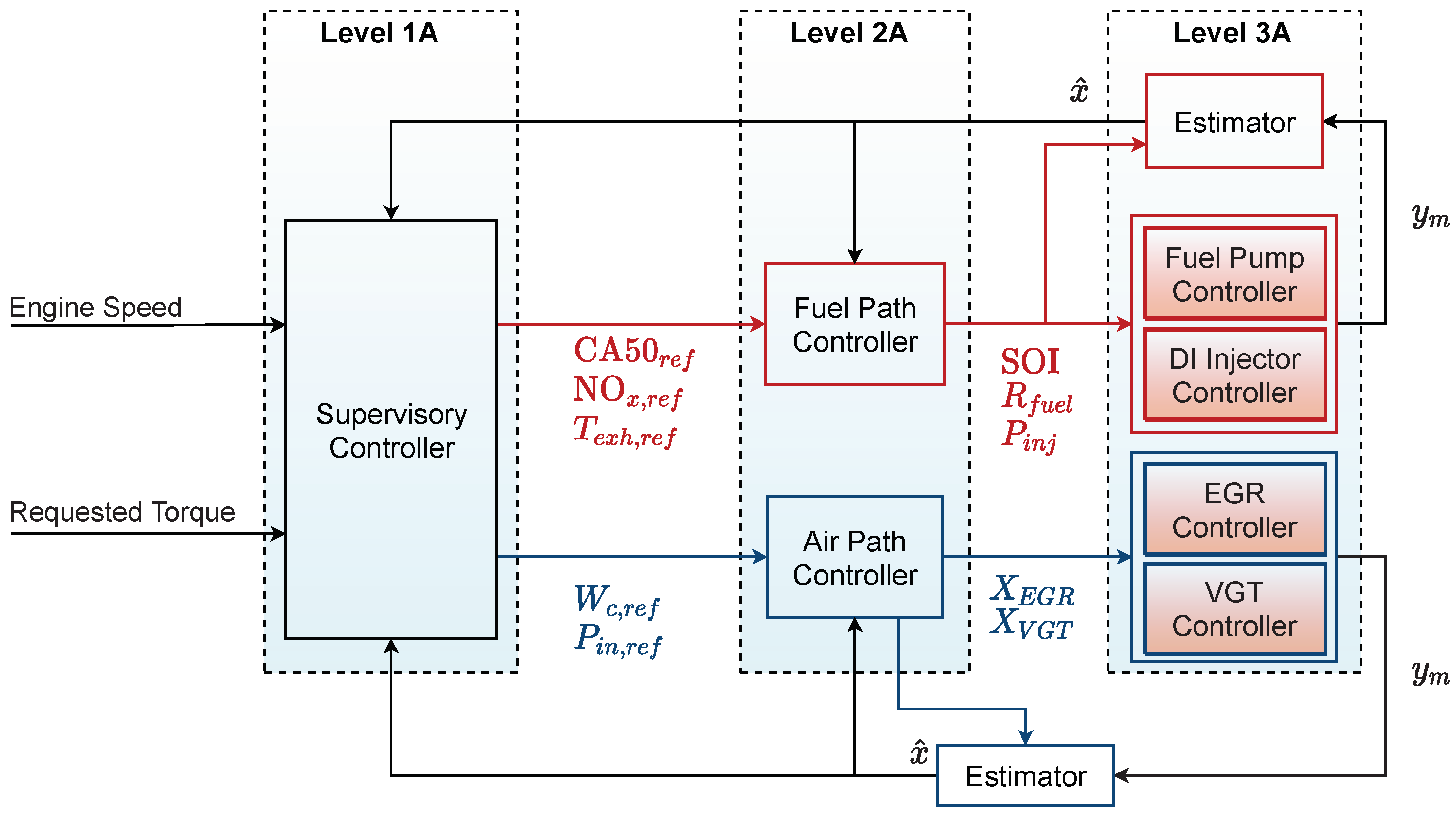
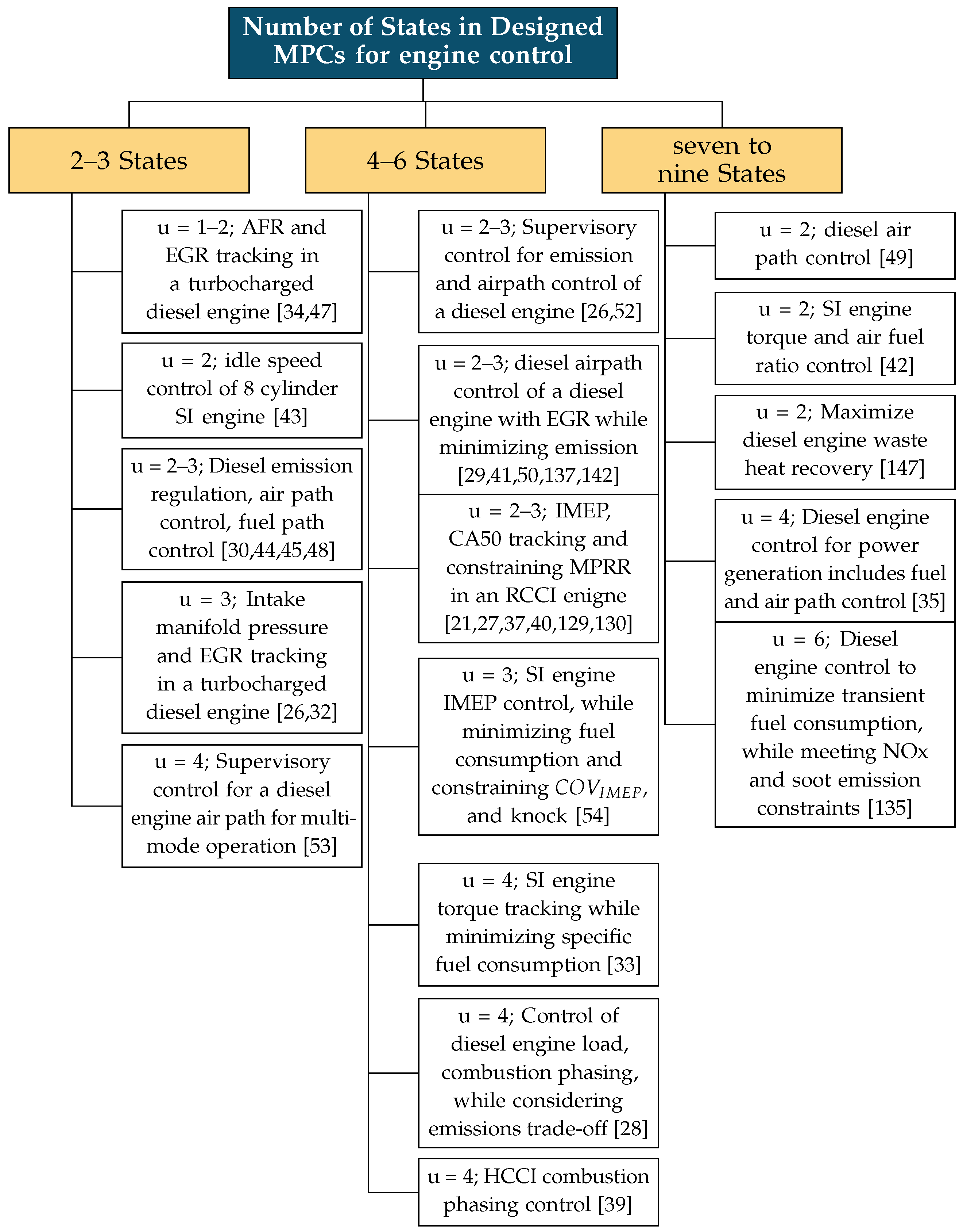
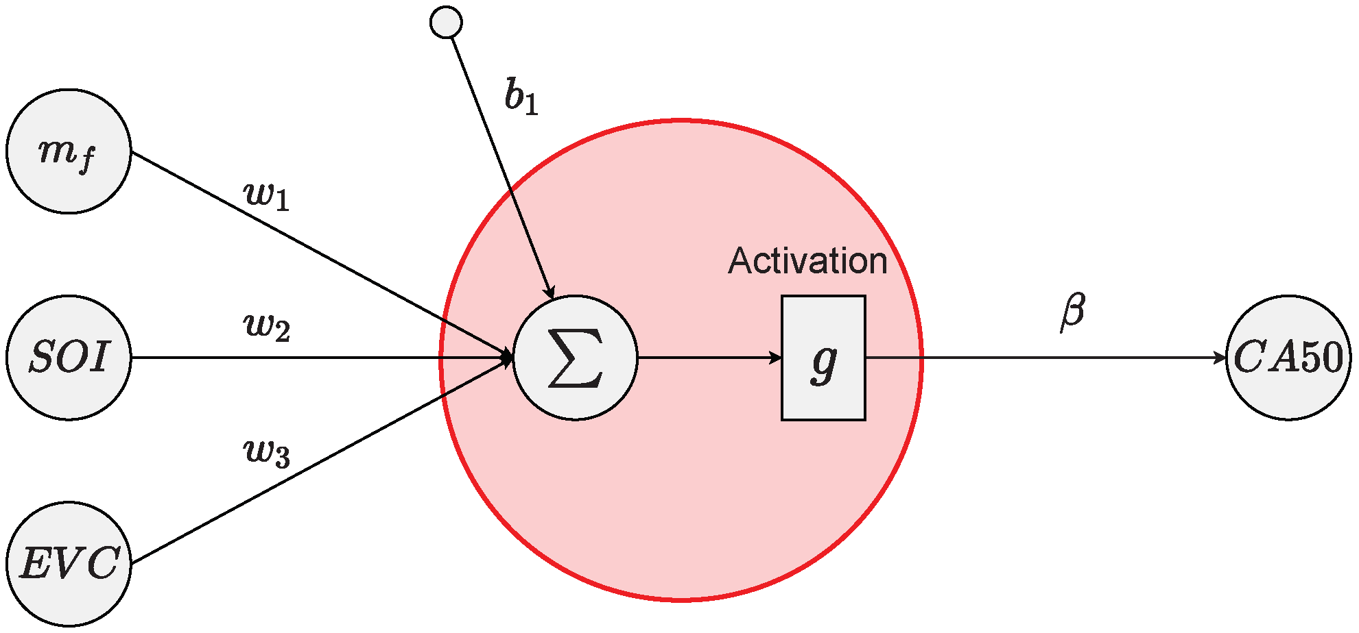
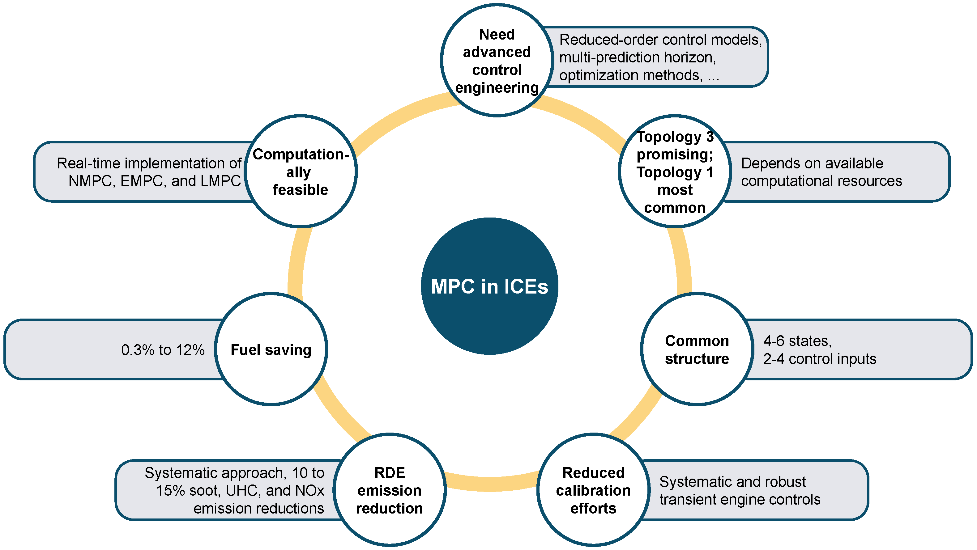
Table 1.
Types of MPC controllers used in the literature that are demonstrated for ICE controls.
| MPC Types | Experimental | Simulation | Processor-In-Loop (PIL) | |
|---|---|---|---|---|
| Linear | Explicit | [30,38,39,40,43,45,47,50] | – | – |
| Single | [24,28,36,37,40,49] | [108,142,145,151] | – | |
| Switching | [27,29,33,46,53] | [147,149] | – | |
| LPV | [21,29,42,48] | [22,129,143,150] | – | |
| Economic | Linear | [35] | – | – |
| Nonlinear | [52,54,136] | [137] | – | |
| Nonlinear | – | [26,32,34,41,51] | [130,138,139,140,141,144,148,150] | [135] |
Table 2.
Classification of ICE control problems based on the engine model and optimization problem.
| Problems | Control Applications |
|---|---|
| Multi linear | Waste heat recovery [147,149] |
| Burn rate/combustion phasing [21,22,27,28,37,38,39,108,129] | |
| Torque and IMEP [22,27,28,33,35,37,38,39,40,42,108] | |
| Idle speed [25,36,43,140] | |
| Convex or convexifiable | NOx emission [26,28,30,137] |
| Exhaust aftertreatment system [145] | |
| Combustion mode transition [53] | |
| Airpath of turbocharged engines [32,34,52,141,144] | |
| Non-Convex | Cyclic Variability [54,152] |
| Soot and uHC emissions [153,154] | |
| Knock and MPRR [155,156,157] |
Table 3.
Common solvers for MPC along with the application type, optimization method, and availability of open source).
Table 3.
Common solvers for MPC along with the application type, optimization method, and availability of open source).
| Optimization Solver | MPC Problem Type | Optimization | Commercial/Free |
|---|---|---|---|
| IPOPT * [171] | LMPC, Convex NMPC, Nonconvex NMPC | IP | F |
| BARON [172] | LMPC, Convex NMPC, Nonconvex NMPC | IP, SQP | C |
| Gurobi [173] | LMPC, Convex NMPC, Nonconvex NMPC | IP | C |
| ForcesPro [169,174] | LMPC, Convex NMPC, Nonconvex NMPC | IP, SQP, FOM | C |
| SNOPT * [175] | LMPC, Convex NMPC, Nonconvex NMPC | IP, SQP | C |
| OOQP [176] | LMPC | IP | F |
| duQuad [177] | LMPC, Convex NMPC | FOM | F |
| HPIPM [178] | LMPC, Convex NMPC | IP | F |
| qpOASES * [179] | LMPC, Convex NMPC, Nonconvex NMPC | SQP | F |
| OpEn [179] | LMPC, Convex NMPC, Nonconvex NMPC | AGD | F |
| WORHP * [180] | LMPC, NMPC | SQP, IP | C |
| CPLEX [181] | LMPC, Convex NMPC | C | |
| CVXOPT [182] | LMPC, Convex NMPC | IP | F |
| KNITRO * [183] | LMPC, Convex NMPC, Nonconvex NMPC | IP, SQP | C |
| Mathworks MPC Toolbox * [184] | LMPC, NMPC | C | |
| FiOrdOs [185] | LMPC | FOM | F |
| APOPT [186] | LMPC, Convex NMPC | SQP | F |
| LOQO [187] | LMPC, Convex NMPC, Nonconvex NMPC | IP, SQP | C |
| OnRAMP (Honeywell) * | LMPC, Convex NMPC, Nonconvex NMPC | C | |
| YALMIP * [188] | LMPC, Convex NMPC, Nonconvex NMPC | IP, SQP | F |
| ACADO * [189] | LMPC, Convex NMPC, Nonconvex NMPC | IP, SQP | F |
* Implemented in ICE application.
Table 4.
Problem size and execution time for MPC controllers reported in [26]—ECU execution times are estimated for a 256 MHz ECU clocking scaling.
Table 4.
Problem size and execution time for MPC controllers reported in [26]—ECU execution times are estimated for a 256 MHz ECU clocking scaling.
| Supervisory SMPC | NMPC Feedforward | NMPC Feedback | |
|---|---|---|---|
| Average execution time [s] | 530 | 31 | 127 |
| Maximum execution time [s] | 550 | 32 | 133 |
| Maximum estimated ECU execution time [ms] | 5.6 | 0.33 | 1.5 |
| Number of decision variables | 17 | 18 | 18 |
| Number of hard constraints | 41 | 0 | 0 |
Table 5.
Summary of the main accomplishments of articles reviewed about MPC in ICEs in comparison with conventional control methods.
Table 5.
Summary of the main accomplishments of articles reviewed about MPC in ICEs in comparison with conventional control methods.
| Achievements | References |
|---|---|
| Fuel Saving (0.3 to 12%) | [26,28,29,34,35,36,47,52,54,135,136,137] |
| NOx reduction (up to 15%) | [26,28,30,41,45,47,135,137,145] |
| PM reduction (up to 11%) | [29,47,137] |
| HC reduction (10 to 15%) | [26] |
| Calibration effort reduction | [36,46,52,53] |
| Tracking improvement (up to 40%) | [21,22,25,26,27,28,29,30,31,32,33,34,35,36,37,38,39,40,41,42,43,44,45,46,47,48,49,50,51,52,53,54,108,136,137,138,139,140,141,142,143,144,147,148,149,150,151] |
Publisher’s Note: MDPI stays neutral with regard to jurisdictional claims in published maps and institutional affiliations. |
© 2021 by the authors. Licensee MDPI, Basel, Switzerland. This article is an open access article distributed under the terms and conditions of the Creative Commons Attribution (CC BY) license (https://creativecommons.org/licenses/by/4.0/).
Share and Cite
MDPI and ACS Style
Norouzi, A.; Heidarifar, H.; Shahbakhti, M.; Koch, C.R.; Borhan, H. Model Predictive Control of Internal Combustion Engines: A Review and Future Directions. Energies 2021, 14, 6251. https://doi.org/10.3390/en14196251
AMA Style
Norouzi A, Heidarifar H, Shahbakhti M, Koch CR, Borhan H. Model Predictive Control of Internal Combustion Engines: A Review and Future Directions. Energies. 2021; 14(19):6251. https://doi.org/10.3390/en14196251
Chicago/Turabian StyleNorouzi, Armin, Hamed Heidarifar, Mahdi Shahbakhti, Charles Robert Koch, and Hoseinali Borhan. 2021. "Model Predictive Control of Internal Combustion Engines: A Review and Future Directions" Energies 14, no. 19: 6251. https://doi.org/10.3390/en14196251
Note that from the first issue of 2016, this journal uses article numbers instead of page numbers. See further details here.