
Power Plant Energy Predictions Based on Thermal Factors Using Ridge and Support Vector Regressor Algorithms
by
 , and
, and
Asif Afzal
1,2,* ,
,
Saad Alshahrani
3,
Abdulrahman Alrobaian
4,
Abdulrajak Buradi
5,* and
Sher Afghan Khan
6 1
Department of Mechanical Engineering, P. A. College of Engineering (Affiliated to Visvesvaraya Technological University, Belagavi), Mangaluru 574153, India
2
Department of Mechanical Engineering, School of Technology, Glocal University, Delhi-Yamunotri Marg, SH-57, Mirzapur Pole, Saharanpur District, Uttar Pradesh 247121, India
3
Department of Mechanical Engineering, College of Engineering, King Khalid University, P.O. Box 394, Abha 61421, Saudi Arabia
4
Department of Mechanical Engineering, College of Engineering, Qassim University, Buraydah 51452, Saudi Arabia
5
Department of Mechanical Engineering, Nitte Meenakshi Institute of Technology, Bangalore 560064, India
6
Department of Mechanical Engineering, Faculty of Engineering, International Islamic University, Kuala Lumpur 50728, Malaysia
*
Authors to whom correspondence should be addressed.
Energies 2021, 14(21), 7254; https://doi.org/10.3390/en14217254
Submission received: 11 October 2021
/
Revised: 27 October 2021
/
Accepted: 28 October 2021
/
Published: 3 November 2021
(This article belongs to the Special Issue Dynamic Control and Machine Learning for Thermal Management, Energy Utilization, and Environment)
Abstract
:This work aims to model the combined cycle power plant (CCPP) using different algorithms. The algorithms used are Ridge, Linear regressor (LR), and upport vector regressor (SVR). The CCPP energy output data collected as a factor of thermal input variables, mainly exhaust vacuum, ambient temperature, relative humidity, and ambient pressure. Initially, the Ridge algorithm-based modeling is performed in detail, and then SVR-based LR, named as SVR (LR), SVR-based radial basis function—SVR (RBF), and SVR-based polynomial regression—SVR (Poly.) algorithms, are applied. Mean absolute error (MAE), R-squared (R2), median absolute error (MeAE), mean absolute percentage error (MAPE), and mean Poisson deviance (MPD) are assessed after their training and testing of each algorithm. From the modeling of energy output data, it is seen that SVR (RBF) is the most suitable in providing very close predictions compared to other algorithms. SVR (RBF) training R2 obtained is 0.98 while all others were 0.9–0.92. The testing predictions made by SVR (RBF), Ridge, and RidgeCV are nearly the same, i.e., R2 is 0.92. It is concluded that these algorithms are suitable for predicting sensitive output energy data of a CCPP depending on thermal input variables.

1. Introduction
Electricity is the leading driving soul of current civilization and is the key essential resource to human accomplishments. We require a considerable amount of electrical power for the proper functioning of the economy and our society. Due to the continuous demand for electricity, the number of combined cycle power plants (CCPP) increases day by day. Power plants are established on a large scale to provide the needed amount of electricity. The critical concern is producing electrical power by maintaining a reliable power generation system. In thermal power plants generally, thermodynamical methods are used to analyze the systems accurately for their operation. This method uses many assumptions and parameters to solve thousands of nonlinear equations; its elucidation takes too much effort and computational time. Sometimes, it is not easy to solve these equations without these assumptions [1,2]. To eradicate this barrier, machine learning (ML) methods are common substitutes for thermodynamical methods and mathematical modeling to study random output and input patterns [1]. In the ML approach, envisaging an actual value called regression is the most common problem. The ML approach uses ML algorithms to control the system response and predict an actual numeric value. Many realistic and everyday problems can be elucidated as regression problems to improve predictive models [3].
Artificial Neural Networks (ANNs) are one of the methods of ML. Using ANNs, the environmental conditions and nonlinear relationships are considered inputs of the ANNs model, and the power generated is considered the model’s output. Using the ANNs model, we can calculate the power output of the power plant by imputing various environmental conditions. ANNs were proposed originally in the mid 20th century as a human brain computational model. At that time, their use was restricted due to the availability of limited computational power and a few theoretically unsolved problems. They have been applied and studied increasingly recently due to availability of computational power and datasets [4]. In modern thermal power plants, a massive quantity of parametric data is kept over long periods; hence, big data created on the active data is continuously readily available without extra cost [2]. Using the ANNs model in [1], various effects such as wind velocity and its direction, relative humidity, ambient pressure, and the ambient temperature of the power plant are examined based on the measured information from the power plant. For varying local atmospheric conditions, in [5], the ANNs model is used to calculate the performance and operational parameters of a Gas Turbine (GT). In [6], researchers compare different ML methods to calculate the total load output of electrical power of a baseload operated CCPP. The modeling of stationary GT is also done by using ANNs. In [7], the ANNs system is developed and effectively used for studying the behaviors of GT for different ranges of working points starting from full speed full load and no-load situations. The Radial Basis Function (RBF) and Multi-Layer Perception (MLP) networks are effectively used in [8] for finding the startup stage of stationary GT. In [9,10], the authors used different designs of the MLP method to estimate the electrical power output and performance of the CCPP by using variable solvers, hidden layer configurations, and activation functions.
The output power of GT mainly depends on atmospheric parameters such as relative humidity, atmospheric pressure, and atmospheric temperature. The output power of a steam turbine (ST) has a direct correlation with exhaust vacuum. The effects of atmospheric disorders are considered in the literature to calculate electrical power (PE) using ML intelligence systems, i.e., ANNs [1,5]. For identification of GT, in [11], the Feed Forward Neural Networks (FFNNs) and dynamic linear models are compared and found Neural Networks (NNs) as a prognosticator model to pinpoint special enactments than the vigorous linear models. The ANNs models are also effectively employed in isolation, fault detection, anomaly detection, and performance analysis of GT engines [2,12,13,14]. In [12,15,16], CCPP’s total electrical energy power output is predicted using FFNNs entirely based on a novel trained particle swarm optimization method. Atmospheric pressure, vacuum, relative humidity, and ambient temperature are used as input factors to calculate the hourly average power output of the CCPP. An ANNs-based ML processing tool and its predictive approach are successfully used in [17] CCPPs to study and analyze the environmental impact on CCPP generation. In [18], the Internet of Things (IoT) based micro-controller automatic information logger method is employed to accumulate environmental data in CCPPs. In [19], the researchers estimate the electrical power output by employing the Genetic Algorithm (GA) method for the design of multi-layer perception (MLP) for CCPPs.
Yu et al. [20] developed an enhanced combined power and heat economic dispatch (CPHED) model for natural gas CCPP. In addition, the authors examined the effect of heat load ramp rates on CPHED, which can deliver guidance and theoretical support for field operation. The study shows that the error among the field operational data and short term loads deviation model are less than 1 s on heat load and less than 2.6 s on power load, which proves the model’s accuracy. The authors also suggested that the enhanced CPHED model improves the operational reliability and improves the economic performance of plants. Wood [21] used the transparent, open box (TOB) ML technique or algorithm to calculate an accurate electrical output power (EOP) and to calculate the errors for a combined cycle gas turbine (CCGT) power plant. Using the TOB algorithm, the authors revealed that a ML tool could produce exact calculations. To optimize using the TOB algorithm, the authors revealed that an ML tool is more capable of producing exact calculations optimizing CCGT performance and its efficiency. Hundi and Shahsavari [22] performed different proportional studies between ML models assess performance and monitor the health of CCPP. The authors modeled the full load O/P power of the plant by using atmospheric pressure (AP), exhaust vacuum pressure (EVP), ambient temperature (AT), and relative humidity (RH) as I/P variables by applying support vector machines, ANNs, random forests, and linear regression. The authors suggested that the methods used in their study help in allowing better control over day-to-day processes and reliable forecasting and monitoring of hourly energy O/P. Aliyu et al. [23] performed a detailed thermodynamic (exergy and energy) analysis of a CCPP using the design data. The authors used a triple pressure CCPP furnished with reheat facilities and determined the exergy destruction and temperature gradient through each heat retrieval steam generator device. The authors also revealed that the steam quality, reheat pressure, and superheat pressure at the outlet of the low-pressure ST expressively disturbs the efficiencies and O/P of the turbine.
Karacor et al. [24] used and generated life performance models to enhance the effective use of energy for a CCPP of 243 MW using ANNs and the fuzzy logic (FL) technique. The study results revealed that the estimation of energy relative error produced among the years estimated in modeling by using ANNs varies between 0.001% and 0.84% and is found to vary variesbetween 0.59% and 3.54% in modeling using ANNs. The study also revealed that the ANNs model is more appropriate for estimating the lifetime performance of a nonlinear system. Rabby Shuvo et al. [25] successfully used the four different ML regression methods to predict and forecast the total energy O/P in CCPPs hourly. The study shows that the linear regression (LR) model executes more proficiently than random forest, Linear, and decision tree ML methods in performing the data sets. The authors also found that the value of R2 for LR is about 0.99910896 (99.91%). Zaaoumi et al. [26] used ANNs and analytical models to predict a parabolic trough solar thermal power plant (PTSTPP). The study results revealed that the ANNs model achieves better results than the analytical models. The results of the ANNs model reveal that the predicted yearly electrical energy is about 42.6 GWh/year, whereas the operational energy is around 44.7 GWh/year.
Additionally, in the literature, numerous studies [27,28,29,30,31,32] have been performed to envisage consumption of electrical energy by using ML intelligence tools; also tiny studies, i.e., [1] have been carried out related to the calculation of overall electrical power of a CCPP with a heating system, one ST, and three GTs. In [33], the authors used an Extreme Learning Machine (ELM) as the base regression model to analyze the power plant’s performance in a vibrant atmosphere that can update regression models autonomously to react with abrupt or gradual environmental changes. In [34], the authors used Cuckoo Search-based ANNs to predict the output electrical energy of GT and combined steam mechanisms to yield more reliable mechanisms.
Many investigators have conveyed the reliability and feasibility of ANNs models as analysis and simulation tools for different power plant components and processes [35,36,37,38,39,40,41,42]. Comparatively limited studies have considered the use of ST in a CCPP [2,6,43]. this review shows that researchers often modeled power plant data to predict the energy output. Most commonly used algorithms can be briefed as ANNs, MLP, and sometimes combined with GA algorithm. However, the use of SVR-based algorithms to predict the CCPP output energy is not reported. Multiple regression and Ridge algorithms are also limitedly used in literature pertinent to energy data modeling. The current work is aimed to fill this gap by proposing a regression model based on SVR and Ridge algorithm.
Moreover, the different types of SVR algorithms and the effect of the alpha parameter in the Ridge algorithm are rarely seen, which is also covered in this work. Hence, this work comparatively analyzes different algorithms pertinent to the classification and regression part of machine learning to predict CCPP energy output data based on thermal factors as its input. Ridge and SVR-based algorithms are used to model data, and their performance is accessed using different matrics in this work.
2. CCPP System
For the production of electrical energy, a CCPP system is mainly comprised of a gas turbine (GT), steam heat recovery generators (SHRGs), and a steam turbine (ST). In CCPP, the generated electricity in ST by gas in a single combined cycle is repositioned from one ST to another [6]. In CCPP, a GT produces both hot gasses and electrical power (EP). These hot gasses from GT are allowed to pass over the water-cooled heat exchanger (HE) to generate steam and can be used to produce the EP with the help of ST and coupled generator. Over the world, CCPPs are being installed in increasing amounts where a considerable amount of renewable natural gas is available [10]. Figure 1 illustrates the layout of CCPP. For the present study, all the critical data were taken from CCPP-1. The CCPP-1 is deliberated as a small ST generating a capacity of 480 MW and comprises two 160 MW ABB 13E2 GTs and one 160 MW ABB ST with dual pressure SHRGs. In GT, the applied load is very sensitive to atmospheric conditions, mainly atmospheric pressure (AP), relative humidity (RH), and ambient temperature (AT). Also, the load on ST is very sensitive to the vacuum or exhaust steam pressure (ESP). For the present study, both gasses and ST features are interrelated with ambient conditions, and ESP is used as data set and I/P variables. In the data set, the production of EP by gas and STs is considered a critical variable.
All the I/P and critical variables defined below are associated with average hourly data are taken from the measurement at different sensor points are represented in Figure 1. Atmospheric Pressure (AP): These I/P variable data are measured in millibar (mbar) units with a deviation of 992.89 mbar to 1033.30 mbar. Relative Humidity (RH): These I/P variable data being measured in percentage (%) with a deviation of 25.56% to 100.16%. Exhaust Steam Pressure (ESP) or Vacuum (V): ese I/P variable data are measured in cm Hg witha deviation of 25.36 cm Hg to 81.56 cm Hg. Full load EP output: This variable is employed as a primary variable in the dataset and is measured in MW with a deviation of 420.26 MW to 495.76 MW. Ambient Temperature (AT): ese I/P variable data are measured in degrees Celsius (°C) witha deviation of 1.81 °C to 37.11 °C.
The pre-processing of data is a critical process in ML algorithms to obtain quality data that contains reduction, transformation, cleaning, and data integration methods. The data set may vary from 2 to 1000 s of topographies in measurements, which could be irrelevant or redundant. The dataset selection for subset topographies is decreased by removing the irrelevant and redundant topographies from an initial data set. The main aim of the selection of the feature subset is to attain the smallest set of new features. Using the decreased set of new features allows ML algorithms to work faster and more effectively. Therefore, it supports predicting more correctly by rising learning correctness of ML algorithms and edifying result simplicity [20]. The selection of feature subsets by giving a new feature set that involves ‘n’ number of I/P features. A creation or generation of subsets is the main stage in the section of subsets. The search approach can be employed for creating possible subsets features. Theoretically, the current top subset of the new features set may be achieved by measuring all the prospective subset features competing for ‘2n’ likely subsets. This investigation is known as a comprehensive investigation, which is too costly and unrealizable if the new features set contains vast features [21]. Several search procedures are employed to calculate the best subset of the sole features set, which is more realistic, practical, and accessible. Although in the current study, the inclusive search is used as the best technique. Therefore, each mixture feature is tried and marked with a score using ML regression approaches those counterparts a value of the extrapolation accuracy, the best subset.
3. Power Plant Energy Output Data Modeling
3.1. Ridge Regression (RR)
The RR is a technique dedicated to examining multiple regression datathat is multi-collinearity in nature. The RR is also a critical method employed for investigating multiple regression data that suffer from multi-collinearity. When multi-collinearity arises, least-squares appraisals are unbiased, but their alterations are more so they may be distant from the actual value. By totaling a grade of bias to the regression evaluations, RR reduces the standard errors. It is expected that the net result will be to provide more consistent evaluations.
Following the usual representation, assume our regression equation is engraved in its matrix form as:
where, and represent the independent and dependent variables, respectively, represents the errors as residuals, represents the regression coefficients to be measured, and p represents the number of data points.
Once we include the lambda () function in Equation (1), the modified estimated model becomes Equation (2), the model takes account of variance, which is not considered by the general model. After the data is recognized and prepared to be part of L2 regularization, there are stages that one can accept, which are bias, variance trade-off, and standardization and expectations of RR, which are comparable to direct regression.
Additionally, RR model handles a regression problem in which the loss function is the linear least square’s function, and the L2-norm is used for regularization. The strength of regularization; must be a positive float. Regularization enhances the problem’s conditioning and lowers the variance of the estimates. In this model, the alpha parameter determines whether the model responds to regularization; for example, as alpha is increased or decreased, the model responds, and error is reduced. If the visualization exhibits a jagged or erratic plot, the model may not be sensitive to that form of regularization, and a different one is necessary. This alpha (α) value is varied from 0 to 1 in the modeling to understand its effects, in this work.
3.2. Multiple Linear Regression (MLR)
The MLR is also simply called multiple regressions, an arithmetic method that applies numerous descriptive variables to calculate the consequence of a reaction variable. The key aim of MLR is to model the true correlation among dependent and independent variables. In principle, MLR that allows standard minimum squares regression as it comprises more than one descriptive variable. The simplicity of linear regression’s representation makes it an appealing model. We use a linear equation to describe the input values (x) and one projected output value (y). As a result, the input (x) and the output (y) are both numeric. Each input value or column in the linear equation is given one scale factor, termed a coefficient, symbolized by the capital letter A. One more coefficient is also added, giving the line an additional degree of freedom (e.g., going up and down on a 2D plot) and is commonly known as the bias coefficient or as intercept.
The model in Linear regression of a simple problem having a single y and single x, the equation is:
A line in higher dimensions is a plane or a hyper-plane with more than one input (x). So, the representation is made up of the equation appropriate values of and in the above equation.
3.3. Support Vector Regression (SVR)
The support vector regression (SVR) proposes a regression algorithm that supports nonlinear and linear regressions. This technique works on the code of Support Vector Machine (SVM). The SVR varies SVM because SVM is a classifier applied for calculating discrete definite markers. At the same time, SVR is a regressor employed for calculating constant systematic variables. The SVR uses the same idea as SVM for regression issues. The challenge of regression is to create a function that approximates the mapping from an input domain to real numbers based on a training sample. Finding a hyperplane that optimally divides the characteristics into distinct domains is at the heart of SVR. The main premise here is that the further SV points are from the hyperplane, the more likely it is that the points in their respective regions or values will be appropriately fitted (see Figure 2). Because the location of the vectors affects the hyperplane’s position, SV points are vital for computing it.
In SVR, kernel functions are often adopted to transfer the original dataset (linear/nonlinear) onto a higher-dimensional space to make it a linear dataset. As a result, kernel functions are frequently referred to as “generalized dot products.” The linear, polynomial, and RBF (radial basis function) or Gaussian kernels must be differentiated. In general, linear and polynomial kernels take less time and give less accuracy than RBF or Gaussian kernels to draw the hyperplane decision border across classes. Gaussian RBF is another common Kernel technique used in SVR models. The value of an RBF kernel fluctuates with its distance from the origin or a given location.
The RBG Kernel format is mentioned below in the form as:
is the distance between and of Euclidean type. Adopting the original space, the calculation of similarity (dot product) of and .
is used for RBF kernel whose increasing value indicates the model being overfitted and decrease in its values indicates model being under fitted.
4. Performance Assessment
Different performance metrics are selected. Each metrices is individually calculated for training, and testing the model provided numerical values to access the quality of training calculations and algorithm predictions during testing [45,46,47,48,49].
4.1. Mean Absolute Error (MAE)
MAE is a measure of errors among corresponding observations articulating the equivalent phenomenon. The MAE is the absolute variance among the values that are calculated and the actual values. Absolute variance means that it is ignored if the outcome has an undesirable (-ve) sign. Also, the MAE is the average of all absolute errors and gives the O/P. The examples of X versus Y contain evaluations of witnessed versus expected, one method of measurement versus another, and initial time versus subsequent time. The MAE is calculated by:
where:
Number of errors
Add them all absolute errors
Absolute errors.
4.2. R-Square (R2)
The R-square (R2) is an arithmetical measure of fit that specifies how much deviation of a dependent variable is described by the independent variable in a regression model. The R2 is also called the coefficient of determination. This metric offers a sign of in what mANNser good a model fits a given dataset. It specifies how close the calculated values are plotted (i.e., the regression line) to the actual data values. The value of R2 lies between 0 and 1, where 0 shows that this modelis not suitable for the given data, and one shows that the model hysterics seamlessly to the provided dataset. The R2 is measured as:
In the above R2 equation, is the number of data points, and indicate the calculated predictions from the regressors and actual output from CCPP measured from the experiment, respectively. In the statistical study, the negative (–ve) value must be more significant enough to signify a superior precise model that can go up to a maximum equal to 1.
4.3. Median Absolute Error (MeAE)
As the name proposes, the MeAE is a weighted average of the total errors, with the comparative occurrences as the weightage features. The MeAE is mainly interesting since it is vigorous to outliers. The loss is considered by compelling the average of all absolute variances among the expectation and the target. If is the expected value of the ith sample and is the equivalent actual value, then the average absolute error predicted over samples are restricted as follows:
4.4. Mean Absolute Percentage Error (MAPE)
The MAPE is a measure of how accurate a prognosis system is. The MAPE is usually used as a loss function for regression complications and in the classic calculation due to its actual instinctive explanation in terms of relative error. The MAPE is the supreme collective measure employed to prognosis error and works best if there are no limits to the data and no zeros. It measures the correctness as a percentage and can be deliberated as the median absolute percent error for all periods minus actual values separated by absolute values. The MAPE is as follows:
where:
Number of fitted points,
= Actual value,
Forecast value, and
Summation notation.
4.5. Mean Poisson Deviance (MPD)
The MPD measures how well a statistical model fits the data. In MPD, the mean is equivalent to the variance, but in actual practice, the variance is regularly less than the mean (under-dispersed) or greater (overdispersed). It extends the notion of employing the sum of squares of residuals (RSS) in conventional least squares to situations where model-fitting may be done with the greatest certainty. Exponential dispersion and generalized linear models both use it extensively.
The Poisson deviance is given as:
In this equation if , then the term .
The term indicates the calculated mean for observation u represented by the value Which represents the estimated model parameters. The deviation is a measure of how well the model fits the data; if the model fits well, the observed values will be near to their projected means mu i, leading both components in to be small and, therefore, the deviance to be modest.
5. Results and Discussion
The modeling results were obtained using regression algorithms: Ridge (with different alpha α values), linear regression (LR), support vector regressor (SVR) based LR—SVR (LR), SVR based radial basis function—SVR (RBF), and SVR based polynomial regression—SVR (Poly.). The performance assessing parameters like MAE, R2, MeAE, MAPE, and MPD are analyzed comparatively. It should be noted that the regression Ridge is analyzed in detail, and RidgeCV (Ridge cross-validated) model is used only in the last part of this section. The predictor parameter here is the output of electrical energy power (PEO) from the CCPP affected by VE (exhaust vacuum), ABT (ambient temperature), REH (relative humidity), and ABP (ambient pressure). These readings of CCPP were recorded experimentally, and the entire data set is openly available in the UCI machine learning repository made available by the work reported in [50].
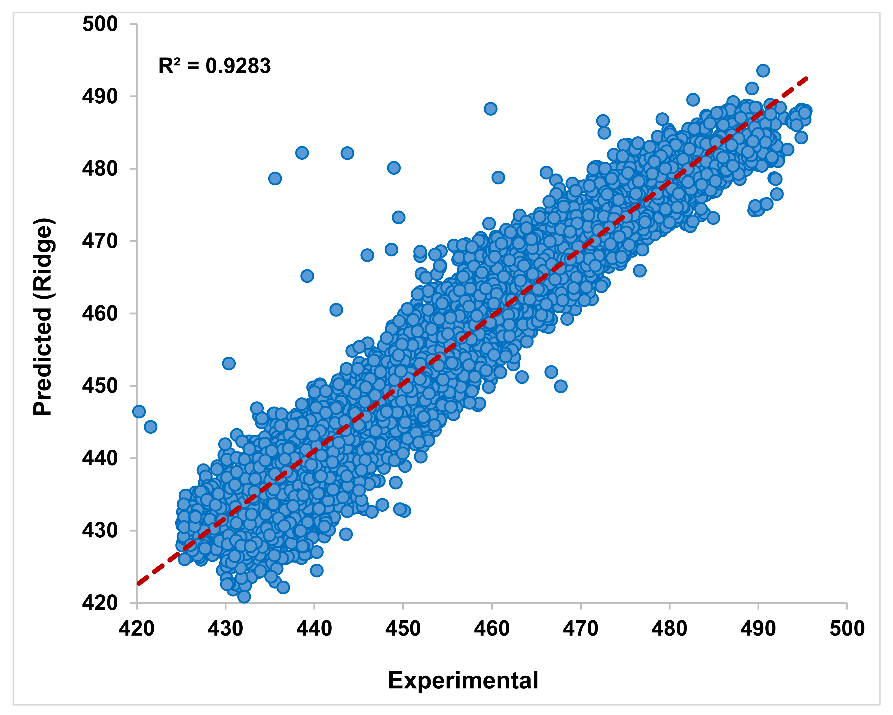
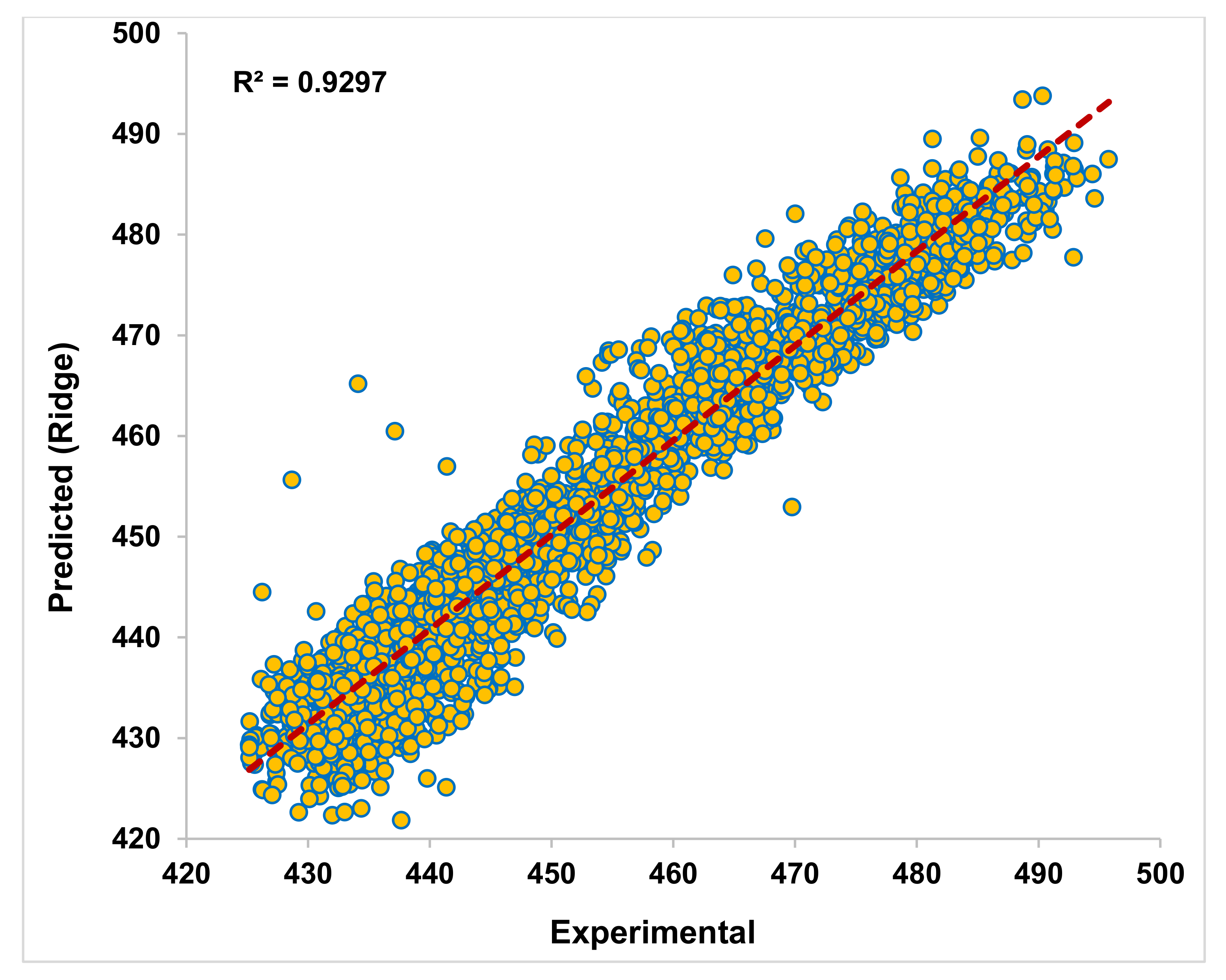
In Figure 3, the Ridge regressor used for modeling PEO data with alpha α = 0, considering only the training output. The training data set of PEO is chosen randomly with a state of 42 for all the models. The training of the Ridge regressor indicates that the obtained output from the algorithm conveniently matches the experimental readings. The trendline shown in the figure indicates that the maximum data obtained from the regressor output is in line with the recorded data. The prime indicator R2 = 0.9283 shows that the training is successful as the value is close to unity. Upon this comfortable training of the Ridge regressor, an attempt is made to test the ability of this model to predict the testing data. From Figure 4, the predictions made by the regressor indicate the output is in an excellent match with the experimental readings. The predictions are even better than the trained output from the regressor. The compactness and closeness with the trendlines indicate this algorithm’s ability to predict power plant energy output based on thermal parameters. Though the data is highly nonlinear, the Ridge model is successful in its predictions. The R2 = 0.9297 during testing is obtained from this regressor, indicating closeness to its perfect unity. For α = 0.2 to 1.0, the training and testing results are avoided for brevity purposes.
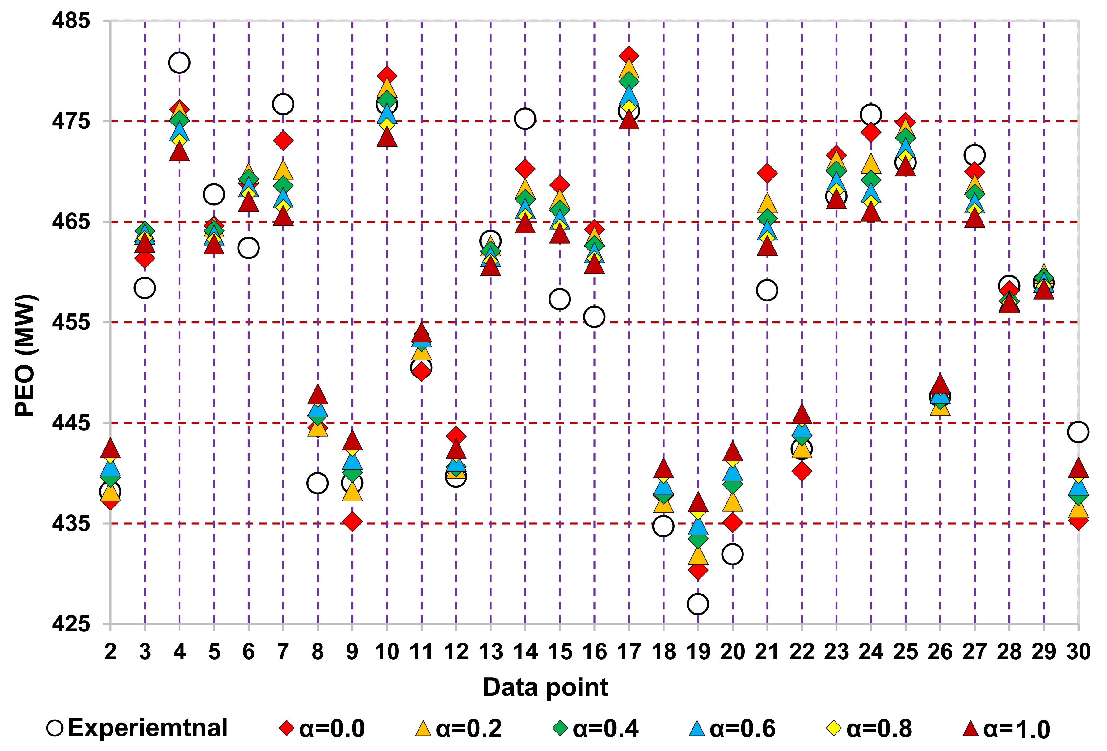
In Figure 5, a better elucidation of predictions made by the Ridge regressor for selected data points is provided. A comparative analysis is shown between the experimental readings and Ridge regressor training outputs with α values ranging from 0 to 1.0. Only the first 30 data points are considered for the demonstration purpose. The figure shows that the trend line of experimental readings with data points and the Ridge regressor trends with α values ranging from 0 to 1.0 are closely placed. The trendlines are sometimes overlapped, making it challenging to make a note of the difference. However, from a close view of the figure, it can be seen that during the high and low peaks, the most closeness between experimental data and predictions from Ridge regressor is at α = 0. As the α value is increased from 0 to 1.0, the tendency to predict the PEO slightly diminishes, i.e., moves slightly away from the actual values. The main reason for this is that the data shrinkage increases with an increase in α value, impacting the coefficients to zero. Figure 6 shows the trends of experimental data opted for testing the trained Ridge regressor, which provides predictions at different α values. Each vertical line represents a data point along which the experimental data and Ridge regressor predictions in the form of scattered data points are shown at different α values. It is seen that the empty circles representing experimental points and diamond in red (α = 0) are very close to other models.
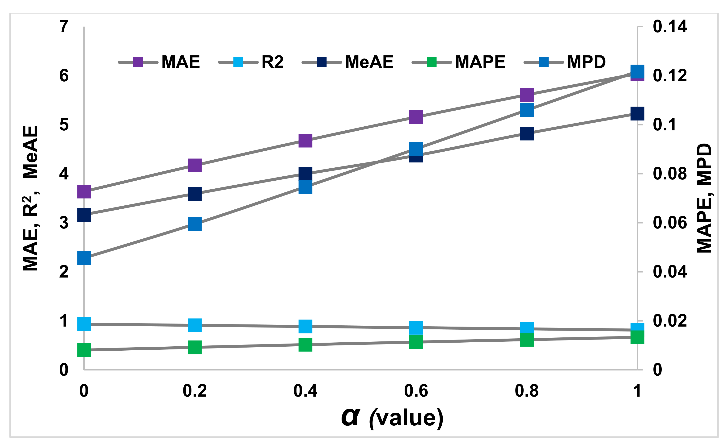
In Figure 7, the performance metrics (MAE, R2, MeAE, MAPE, and MPD) of the Ridge regressor at different α values are shown. This performance of the Ridge regressor is obtained from the training data set computed following experimental data. From the figure, the MAE value is seen rising linearly with the α values. As discussed, the increase in α values impacts the data shrinkage growth; the MAE tends to increase accordingly. The R2 value also indicates that the increase in α values hampers the accuracy of the Ridge regressor. However, the best closet value of R2 obtained is at α = 0. The R2 looks to be a very uniform thought, but a closer look reveals that its value is decreasing, which is unacceptable. The MaAE, MAPE, and MPD metrics also increase with an increase in α values as the training ability of the regressor deteriorates. In Figure 8, the trend of all the metrics is shown with an increase in α values obtained from the testing session. As expected, the performance of the Ridge regressor has worsened with the α values, as also observed from the training data set. However, the metrics are seen to linearly increase with the α values, not in the previous metrics.
Figure 9 shows the Linear regressor obtained output during the training of PEO data of a CCPP. The comparison along the trendline between Linear regressor calculated output and experimental readings are along a line that clearly shows a match among them. The training can be appropriate and successful as the data points are compact, except that a few are outside the region. Such outliers are common in data modeling, which is acceptable as the value of R2 is above 0.9. This training is performed using 90% of the total data available for training purposes. The remaining 10% of data being used to test the model, which is trained using this 90% data. The testing of the Linear regressor model is carried out with the 10% of data, and a comparative plot obtained with experimental data is shown in Figure 10. Significantly few data points fall outside the clustered region, where most of the data points are close to the trendline. The testing of the Linear regressor model depicts that it is also as suitable as the Ridge model in the prediction of PEO of a CCPP. The R2 is above 0.9 in testing results, clearly showing that the Linear regressor model can give a very close result. This indicates that more computational cost and time can be saved by adopting this simple model than other models. In Figure 11, the performance evaluation of the trained and tested Linear regressor is shown in a 3D bar graph for better illustration. The metrics are very close to each other from training and testing. IN BOTH CASES, the MAE, R2, MeAE, MAPE, and MPD are approximately the same, which is usually rare in most modeling processes. A very close value to zero from MAPE and MPD indicates that the error is less and the difference in predicted and the actual value is also significantly less irrespective of whether the data point numerical value involved is large or less.
In Figure 12, the training and testing of PEO data using support vector regressor (SVR) based LR—SVR (LR) algorithm. The R2 for both cases is shown in the graphs at the top left corner. The densely packed data points indicate the training computations performed successfully, and the testing results also show a comfortable prediction from the SVR (LR) trained. The R2 value for both is above 0.91, indicating a good regression of the power plant energy data. In Figure 13, using the SVR-based RBF—SVR (RBF) algorithm, the training of the data set is most successful in this study. The R2 for SVR (RBF) based training is above 0.98, which is the closest unity obtained. The testing of this regressor is shown in Figure 13b, which also indicates a good prediction. However, these predictions during SVR (RBF) testing are not dominant to other algorithms as the R2 is close to 0.93 as in other cases.
The superior performance of SVR (RBF) is the excellent generalization nature of this algorithm. It is robust to outliers and has tolerance to noise in input data based on the confronted mapping. This algorithm s equivalent in performance to neural networks and neuro inference systems. In Figure 14, the Polynomial regression-based SVR (SVR Poly.) algorithm training and testing results. Figure 14a shows that the training of SVR Poly. The model also is trained well with the given actual data. However, this algorithm is not as competent as the R2 is 0.91, also obtained from previous models. The main drawback observed during the training is the excessive computational time taken by this model for 1 degree of polynomial functions. For 3 degrees polynomial functional, the time was not tolerable and did not continue with the training process. Surprisingly, during the testing of this data, the closeness with actual values predicted was slightly better than the training.
In Figure 15, a relative variation of CCPP output energy data from experimental recordings and computed readings using SVR (LR), SVR (RBF), and SVR (Poly.) algorithms is shown. For demonstration, only the first 20 data points are chosen arbitrarily. The circled marker data scattered in the plot shows the experimental values for reference. The reaming empty square boxes show the respective readings computed during the training session of the three SVR algorithms. The SVR (RBF) for most data points completely overlapped, while the other two algorithm readings are seen to deviate but still slightly match the trend of actual values. In Figure 16, the predictions provided by the SVR algorithms during the testing session are comparatively provided. Each vertical line in the figure represents a single data point on which the values from the experiment and SVR algorithms lie. The actual values in an empty brown circle lie in the mid of the SVR readings, majorly predicted data. The closer values seen are from empty yellow triangles, i.e., by SVR (RBF) algorithm. Figure 17a,b the training output computed, and the prediction made from the trained algorithm, respectively. SVR (LR), SVR (RBF), SVR (Poly.), and RidgeCV algorithms are used for comparative analysis. The bars in Figure 17a indicate that the least error is obtained from SVR (RBF). However, during testing Figure 17b, RidgeCV and SVR (RBF) have nearly the same error values.
6. Conclusions
A comparative analysis of modeling of power plant output energy data is examined in this work. Ridge, Linear regression, SVR (LR), SVR (RBF), and SVR (Poly.) algorithms are explored in their capabilities to predict the energy output that depends upon the thermal factors of the power plant. To access the performance of these algorithms, relevant metrics are selected, and the errors in the predictions of these algorithms are comparatively studied. Initially, using Ridge algorithm modeling indicated that it can easily be used for the prediction of energy data. However, for increasing values of α, the Ridge algorithm does not accurately predict the energy data. Linear regression is also equivalently capable of predictions of the data. SVR models have provided an exciting modeling output. SVR linear model has the inline ability with Ridge and Linear regression models. The SVR (RBF) model has given the best training computations, while RBF (Poly.) is a good predictor of this nonlinear sensitive data. The Ridge cross-validated (RidgeCV) algorithm just used for comparison has proved that SVR (RBF) and RidgeCV algorithms are the best among the chosen models in predicting power plant output energy. The performance metrics such as MAE, R2, MeAE, MAPE, and MPD analysis also revealed that the SVR (RBF) is the best algorithm that gives very close predictions to actual values. The following stands are RidgeCV, SVR (Poly.) Ridge, SVR (LR), and then last is the Linear regression model in predictions. This finally indicates that the selected algorithms are well suited for modeling CCPP output energy based on thermal input parameters.
Author Contributions
Conceptualization, A.A. (Asif Afzal); Data curation, A.A. (Abdulrahman Alrobaian) and S.A.K.; Formal analysis, A.A. (Asif Afzal) and A.B.; Funding acquisition, S.A.K.; Investigation, S.A., A.A. (Abdulrahman Alrobaian) and S.A.K.; Methodology, A.A. (Asif Afzal) and A.A. (Abdulrahman Alrobaian); Resources, S.A. and A.B.; Validation, A.B.; Writing—original draft, A.A. (Asif Afzal) and A.B.; Writing—review & editing, S.A. All authors have read and agreed to the published version of the manuscript.
Funding
Deanship of Scientific Research at King Khalid University grant no. R.G.P. 1/132/42.
Institutional Review Board Statement
Not applicable.
Informed Consent Statement
Not applicable.
Data Availability Statement
Not applicable.
Acknowledgments
The authors extend their appreciation to the Deanship of Scientific Research at King Khalid University, Saudi Arabia, for funding this work through the Research Group Program under grant no. R.G.P. 1/132/42.
Conflicts of Interest
The authors declare no conflict of interest.
Nomenclature
| Symbols | Description | Symbols | Description |
| CCPP | Combined cycle power plant | α | Alpha |
| LR | Linear regressor | SHRGs | Steam heat recovery generators |
| SVR | Support vector regressor/regression | EP | Electrical power |
| RBF | Radial basis function | HE | Heat exchanger |
| MAE | Mean absolute error | MW | Mega watt |
| R2 | R-squared | AP | Atmospheric pressure |
| MeAE | Median absolute error | RH | Relative humidity |
| MAPE | Mean absolute percentage error | AT | Ambient temperature |
| MPD | Mean poison deviance | ESP | Exhaust steam pressure |
| CV | Cross-validated | I/P | Input |
| ML | Machine learning | O/P | Output |
| ANNs | Artificial neural networks | RR | Ridge regression |
| GT | Gas turbine | MLR | Multiple linear regression |
| MLP | Multi-layer perception | VE | Exhaust vacuum |
| ST | Steam turbine | RidgeCV | Ridge cross-validated |
| PE | Electrical power | ABT | Ambient temperature |
| FFNNs | Feed forward neural networks | REH | Relative humidity |
| NNs | Neural networks | MLP | Multi-layer perception |
| IoT | Internet of things | ELM | Extreme learning machine |
| GA | Genetic algorithm | SVM | Support vector machines |
| EEP | Electrical energy power | ||
| Symbols | |||
| X | Independent variable | Absolute errors | |
| Y | Dependent variable | n | Number of data points |
| e | Errors | Calculated predictions from regressors | |
| B | Regression coefficient | Calculated actual O/P | |
| x | Input value | Expected value of ith sample | |
| y | Output value | Equivalent actual value | |
| A0, A1 | Scale factors | Actual value | |
| σ | Radial basis function kernel | Ft | Forecast value |
| A1, A2 | Linear datasets | Calculated mean | |
| p | Number of errors | Observed value | |
| Summation of all absolute errors | PD | Poisson deviance | |
References
- Kesgin, U.; Heperkan, H. Simulation of thermodynamic systems using soft computing techniques. Int. J. Energy Res. 2005, 29, 581–611. [Google Scholar] [CrossRef]
- Dehghani Samani, A. Combined cycle power plant with indirect dry cooling tower forecasting using artificial neural network. Decis. Sci. Lett. 2018, 7, 131–142. [Google Scholar] [CrossRef]
- Altay Guvenir, H.; Uysal, I. Regression on feature projections. Knowl. Based Syst. 2000, 13, 207–214. [Google Scholar] [CrossRef] [Green Version]
- Hagan, M.T.; Demuth, H.B.; De Jesús, O. An introduction to the use of neural networks in control systems. Int. J. Robust Nonlinear Control 2002, 12, 959–985. [Google Scholar] [CrossRef]
- Fast, M.; Assadi, M.; De, S. Development and multi-utility of an ANN model for an industrial gas turbine. Appl. Energy 2009, 86, 9–17. [Google Scholar] [CrossRef]
- Tüfekci, P. Prediction of full load electrical power output of a base load operated combined cycle power plant using machine learning methods. Int. J. Electr. Power Energy Syst. 2014, 60, 126–140. [Google Scholar] [CrossRef]
- Rahnama, M.; Ghorbani, H.; Montazeri, A. Nonlinear identification of a gas turbine system in transient operation mode using neural network. In Proceedings of the 4th Conference on Thermal Power Plants; IEEE, Teheran, Iran, 18–19 December 2012; pp. 1–6. [Google Scholar]
- Refan, M.H.; Taghavi, S.H.; Afshar, A. Identification of heavy duty gas turbine startup mode by neural networks. In Proceedings of the 4th Conference on Thermal Power Plants, Teheran, Iran, 18–19 December 2012; pp. 1–6. [Google Scholar]
- Lorencin, I.; Car, Z.; Kudláček, J.; Mrzljak, V.; Anđelić, N.; Blažević, S. Estimation of combined cycle power plant power output using multilayer perceptron variations. In Proceedings of the 10th International Technical Conference—Technological Forum 2019, Hlinsko, Czech Republic, 18–20 June 2019. [Google Scholar]
- Islikaye, A.A.; Cetin, A. Performance of ML methods in estimating net energy produced in a combined cycle power plant. In Proceedings of the 6th International Istanbul Smart Grids and Cities Congress and Fair (ICSG), Istanbul, Turkey, 25–26 April 2018; pp. 217–220. [Google Scholar] [CrossRef]
- Yari, M.; Aliyari Shoorehdeli, M.; Yousefi, I. V94.2 gas turbine identification using neural network. In Proceedings of the First RSI/ISM International Conference on Robotics and Mechatronics (ICRoM), Teheran, Iran, 13–15 February 2013; pp. 523–529. [Google Scholar] [CrossRef]
- Sina Tayarani-Bathaie, S.; Sadough Vanini, Z.N.; Khorasani, K. Dynamic neural network-based fault diagnosis of gas turbine engines. Neurocomputing 2014, 125, 153–165. [Google Scholar] [CrossRef]
- Kumar, A.; Srivastava, A.; Banerjee, A.; Goel, A. Performance based anomaly detection analysis of a gas turbine engine by artificial neural network approach. In Proceedings of the Annual Conference of the Prognostics and Health Management Society, Minneapolis, MN, USA, 23–27 September 2012; pp. 450–457. [Google Scholar]
- Rashid, M.; Kamal, K.; Zafar, T.; Sheikh, Z.; Shah, A.; Mathavan, S. Energy prediction of a combined cycle power plant using a particle swarm optimization trained feedforward neural network. In Proceedings of the International Conference on Mechanical Engineering, Automation and Control Systems (MEACS), Tomsk, Russia, 1–4 December 2015; pp. 27–31. [Google Scholar] [CrossRef]
- Akdemir, B. Prediction of hourly generated electric power using artificial neural network for combined cycle power plant. Int. J. Electr. Energy 2016, 4, 91–95. [Google Scholar] [CrossRef]
- Elfaki, E.A.; Ahmed, A.H. Prediction of electrical output power of combined cycle power plant using regression ANN model. J. Power Energy Eng. 2018, 6, 17–38. [Google Scholar] [CrossRef] [Green Version]
- Hassanul Karim Roni, M.; Khan, M.A.G. An artificial neural network based predictive approach for analyzing environmental impact on combined cycle power plant generation. In Proceedings of the 2nd International Conference on Electrical & Electronic Engineering (ICEEE), Rajshahi, Bangladesh, 27–29 December 2017; pp. 1–4. [Google Scholar] [CrossRef]
- Uma, K.; Swetha, M.; Manisha, M.; Revathi, S.V.; Kannan, A. IOT based environment condition monitoring system. Indian J. Sci. Technol. 2017, 10, 1–6. [Google Scholar] [CrossRef] [Green Version]
- Lorencin, I.; Andelić, N.; Mrzljak, V.; Car, Z. Genetic algorithm approach to design of multi-layer perceptron for combined cycle power plant electrical power output estimation. Energies 2019, 12, 4352. [Google Scholar] [CrossRef] [Green Version]
- Yu, H.; Nord, L.O.; Yu, C.; Zhou, J.; Si, F. An improved combined heat and power economic dispatch model for natural gas combined cycle power plants. Appl. Therm. Eng. 2020, 181, 115939. [Google Scholar] [CrossRef]
- Wood, D.A. Combined cycle gas turbine power output prediction and data mining with optimized data matching algorithm. SN Appl. Sci. 2020, 2, 1–21. [Google Scholar] [CrossRef] [Green Version]
- Hundi, P.; Shahsavari, R. Comparative studies among machine learning models for performance estimation and health monitoring of thermal power plants. Appl. Energy 2020, 265, 114775. [Google Scholar] [CrossRef]
- Aliyu, M.; AlQudaihi, A.B.; Said, S.A.M.; Habib, M.A. Energy, exergy and parametric analysis of a combined cycle power plant. Therm. Sci. Eng. Prog. 2020, 15, 100450. [Google Scholar] [CrossRef]
- Karaçor, M.; Uysal, A.; Mamur, H.; Şen, G.; Nil, M.; Bilgin, M.Z.; Doğan, H.; Şahin, C. Life performance prediction of natural gas combined cycle power plant with intelligent algorithms. Sustain. Energy Technol. Assess. 2021, 47. [Google Scholar] [CrossRef]
- Rabby Shuvo, M.G.; Sultana, N.; Motin, L.; Islam, M.R. Prediction of hourly total energy in combined cycle power plant using machine learning techniques. In Proceedings of the 1st International Conference on Artificial Intelligence and Data Analytics (CAIDA), Riyadh, Saudi Arabia, 6–7 April 2021; pp. 170–175. [Google Scholar] [CrossRef]
- Zaaoumi, A.; Bah, A.; Ciocan, M.; Sebastian, P.; Balan, M.C.; Mechaqrane, A.; Alaoui, M. Estimation of the energy production of a parabolic trough solar thermal power plant using analytical and artificial neural networks models. Renew. Energy 2021, 170, 620–638. [Google Scholar] [CrossRef]
- AlRashidi, M.R.; EL-Naggar, K.M. Long term electric load forecasting based on particle swarm optimization. Appl. Energy 2010, 87, 320–326. [Google Scholar] [CrossRef]
- Che, J.; Wang, J.; Wang, G. An adaptive fuzzy combination model based on self-organizing map and support vector regression for electric load forecasting. Energy 2012, 37, 657–664. [Google Scholar] [CrossRef]
- Leung, P.C.M.; Lee, E.W.M. Estimation of electrical power consumption in subway station design by intelligent approach. Appl. Energy 2013, 101, 634–643. [Google Scholar] [CrossRef]
- Kavaklioglu, K. Modeling and prediction of Turkey’s electricity consumption using Support Vector Regression. Appl. Energy 2011, 88, 368–375. [Google Scholar] [CrossRef]
- Azadeh, A.; Saberi, M.; Seraj, O. An integrated fuzzy regression algorithm for energy consumption estimation with non-stationary data: A case study of Iran. Energy 2010, 35, 2351–2366. [Google Scholar] [CrossRef]
- Tso, G.K.F.; Yau, K.K.W. Predicting electricity energy consumption: A comparison of regression analysis, decision tree and neural networks. Energy 2007, 32, 1761–1768. [Google Scholar] [CrossRef]
- Xu, R.; Yan, W. Continuous modeling of power plant performance with regularized extreme learning machine. In Proceedings of the International Joint Conference on Neural Networks (IJCNN), Budapest, Hungary, 14–19 July 2019; pp. 1–8. [Google Scholar] [CrossRef]
- Chatterjee, S.; Dey, N.; Ashour, A.S.; Drugarin, C.V.A. Electrical energy output prediction using cuckoo search based artificial neural network. Smart Trends Syst. Secur. Sustain. 2018, 18, 277–285. [Google Scholar] [CrossRef]
- Bettocchi, R.; Spina, P.R.; Torella, G. Gas Turbine Health Indices Determination by Using Neural Networks. In Proceedings of the ASME Turbo Expo 2002: Power for Land, Sea, and Air. Volume 2: Turbo Expo 2002, Parts A and B, Amsterdam, The Netherlands, 3–6 June 2002; pp. 1083–1089. [Google Scholar] [CrossRef]
- Khosravi, A.; Nahavandi, S.; Creighton, D. Prediction intervals for short-term wind farm power generation forecasts. IEEE Trans. Sustain. Energy 2013, 4, 602–610. [Google Scholar] [CrossRef]
- Mahmoud, T.; Dong, Z.Y.; Ma, J. An advanced approach for optimal wind power generation prediction intervals by using self-adaptive evolutionary extreme learning machine. Renew. Energy 2018, 126, 254–269. [Google Scholar] [CrossRef]
- Wan, C.; Xu, Z.; Pinson, P.; Dong, Z.Y.; Wong, K.P. Optimal prediction intervals of wind power generation. IEEE Trans. Power Syst. 2014, 29, 1166–1174. [Google Scholar] [CrossRef] [Green Version]
- Boccaletti, C.; Cerri, G.; Seyedan, B. A neural network simulator of a gas turbine with a waste heat recovery section. J. Eng. Gas Turbines Power 2001, 123, 371–376. [Google Scholar] [CrossRef]
- Bizzarri, F.; Bongiorno, M.; Brambilla, A.; Gruosso, G.; Gajani, G.S. Model of photovoltaic power plants for performance analysis and production forecast. IEEE Trans. Sustain. Energy 2013, 4, 278–285. [Google Scholar] [CrossRef] [Green Version]
- Huang, H.; Wang, H.; Peng, J. Optimal prediction intervals of wind power generation based on FA-ELM. In Proceedings of the IEEE Sustainable Power and Energy Conference (iSPEC), Chengdu, China, 23–25 November 2020; pp. 98–103. [Google Scholar]
- Erdem, H.H.; Sevilgen, S.H. Case study: Effect of ambient temperature on the electricity production and fuel consumption of a simple cycle gas turbine in Turkey. Appl. Therm. Eng. 2006, 26, 320–326. [Google Scholar] [CrossRef]
- Niu, L.X.; Liu, X.J. Multivariable generalized predictive scheme for gas turbine control in combined cycle power plant. In Proceedings of the 2008 IEEE Conference on Cybernetics and Intelligent Systems, Chengdu, China, 21–24 September 2008; pp. 791–796. [Google Scholar] [CrossRef]
- Kilani, N.; Khir, T.; Ben Brahim, A. Performance analysis of two combined cycle power plants with different steam injection system design. Int. J. Hydrog. Energy 2017, 42, 12856–12864. [Google Scholar] [CrossRef]
- Afzal, A.; Khan, S.A.; Islam, T.; Jilte, R.D.; Khan, A.; Soudagar, M.E.M. Investigation and back-propagation modeling of base pressure at sonic and supersonic Mach numbers. Phys. Fluids 2020, 32, 096109. [Google Scholar] [CrossRef]
- Afzal, A.; Aabid, A.; Khan, A.; Afghan, S.; Rajak, U.; Nath, T.; Kumar, R. Response surface analysis, clustering, and random forest regression of pressure in suddenly expanded high-speed aerodynamic flows. Aerosp. Sci. Technol. 2020, 107, 106318. [Google Scholar] [CrossRef]
- Afzal, A.; Navid, K.M.Y.; Saidur, R.; Razak, R.K.A.; Subbiah, R. Back propagation modeling of shear stress and viscosity of aqueous Ionic-MXene nanofluids. J. Therm. Anal. Calorim. 2021, 145, 2129–2149. [Google Scholar] [CrossRef]
- David, O.; Waheed, M.A.; Taheri-Garavand, A.; Nath, T.; Dairo, O.U.; Bolaji, B.O.; Afzal, A. Prandtl number of optimum biodiesel from food industrial waste oil and diesel fuel blend for diesel engine. Fuel 2021, 285, 119049. [Google Scholar] [CrossRef]
- Mokashi, I.; Afzal, A.; Khan, S.A.; Abdullah, N.A.; Bin Azami, M.H.; Jilte, R.D.; Samuel, O.D. Nusselt number analysis from a battery pack cooled by different fluids and multiple back-propagation modelling using feed-forward networks. Int. J. Therm. Sci. 2021, 161, 106738. [Google Scholar] [CrossRef]
- Kaya, H.; Tüfekci, P.; Gurgen, F. Local and global learning methods for predicting power of a combined gas & steam turbine. In Proceedings of the International Conference on Emerging Trends in Computer and Electronics Engineering ICETCEE, Dubai, United Arab Emirates, 24–25 March 2012; pp. 13–18. [Google Scholar]
Figure 1.
The simple layout of CCPP (reprinted with permission from Elsevier 2017 [44]).
Figure 1.
The simple layout of CCPP (reprinted with permission from Elsevier 2017 [44]).

Figure 2.
Concept of SVR modeling.

Figure 3.
Training results of Ridge regressor with α = 0 with R2 = 0.9283.

Figure 4.
Ridge regressor (α = 0) predicting the PEO with R2 = 0.9297 during testing.

Figure 5.
The trend of experimental readings and predictions made by Ridge regressor for the first 30 data points during training with different α values ranging from 0 to 1.0.
Figure 5.
The trend of experimental readings and predictions made by Ridge regressor for the first 30 data points during training with different α values ranging from 0 to 1.0.

Figure 6.
Scatter data plot of predictions by Ridge regressor at different α values during testing.

Figure 7.
Performance of Ridge regressor at different α values from the training computations (R2 is shown as R2 in the graph legends).
Figure 7.
Performance of Ridge regressor at different α values from the training computations (R2 is shown as R2 in the graph legends).

Figure 8.
Ridge regressor performance metrics change linearly with α values in the tested dataset (R2 is shown as R2 in the graph legends).
Figure 8.
Ridge regressor performance metrics change linearly with α values in the tested dataset (R2 is shown as R2 in the graph legends).

Figure 9.
Training output from Linear regressor and experimental output compared along a line where the R2 is 0.904 from the trendline.
Figure 9.
Training output from Linear regressor and experimental output compared along a line where the R2 is 0.904 from the trendline.

Figure 10.
Testing predictions from Linear regressor and experimental output plotted along a line where the R2 is 0.907 from the trendline.
Figure 10.
Testing predictions from Linear regressor and experimental output plotted along a line where the R2 is 0.907 from the trendline.

Figure 11.
The different forms of errors were analyzed in the Linear regressor obtained from the training and testing points (R2 is shown as R2 in the horizontal x-axis).
Figure 11.
The different forms of errors were analyzed in the Linear regressor obtained from the training and testing points (R2 is shown as R2 in the horizontal x-axis).

Figure 12.
(a) Training and (b) testing of PEO using support vector regressor (SVR) based LR—SVR (LR) algorithm.
Figure 12.
(a) Training and (b) testing of PEO using support vector regressor (SVR) based LR—SVR (LR) algorithm.

Figure 13.
SVR-based radial basis function—SVR (RBF) algorithm (a) Training and (b) testing results for the CCPP energy output.
Figure 13.
SVR-based radial basis function—SVR (RBF) algorithm (a) Training and (b) testing results for the CCPP energy output.

Figure 14.
Polynomial regression-based SVR (SVR Poly.) algorithm used for (a) Training and (b) testing of PEO data.
Figure 14.
Polynomial regression-based SVR (SVR Poly.) algorithm used for (a) Training and (b) testing of PEO data.

Figure 15.
Comparison between the actual readings of CCPP energy output (PEO) and trained values produced from computations of SVR (LR), SVR (RBF), and SVR (Poly.) algorithms during the training indicating first 20 data points only.
Figure 15.
Comparison between the actual readings of CCPP energy output (PEO) and trained values produced from computations of SVR (LR), SVR (RBF), and SVR (Poly.) algorithms during the training indicating first 20 data points only.

Figure 16.
The predicted data of CCPP using SVR (LR), SVR (RBF), and SVR (Poly.) algorithms were obtained after testing in comparison with experimental readings.
Figure 16.
The predicted data of CCPP using SVR (LR), SVR (RBF), and SVR (Poly.) algorithms were obtained after testing in comparison with experimental readings.

Figure 17.
Assessment of SVR (LR), SVR (RBF), and SVR (Poly.) algorithms compared with RidgeCV used for (a) training and (b) testing of energy output data. (R2 is shown as R2 in the graph legend).
Figure 17.
Assessment of SVR (LR), SVR (RBF), and SVR (Poly.) algorithms compared with RidgeCV used for (a) training and (b) testing of energy output data. (R2 is shown as R2 in the graph legend).

Publisher’s Note: MDPI stays neutral with regard to jurisdictional claims in published maps and institutional affiliations. |
© 2021 by the authors. Licensee MDPI, Basel, Switzerland. This article is an open access article distributed under the terms and conditions of the Creative Commons Attribution (CC BY) license (https://creativecommons.org/licenses/by/4.0/).
Share and Cite
MDPI and ACS Style
Afzal, A.; Alshahrani, S.; Alrobaian, A.; Buradi, A.; Khan, S.A. Power Plant Energy Predictions Based on Thermal Factors Using Ridge and Support Vector Regressor Algorithms. Energies 2021, 14, 7254. https://doi.org/10.3390/en14217254
AMA Style
Afzal A, Alshahrani S, Alrobaian A, Buradi A, Khan SA. Power Plant Energy Predictions Based on Thermal Factors Using Ridge and Support Vector Regressor Algorithms. Energies. 2021; 14(21):7254. https://doi.org/10.3390/en14217254
Chicago/Turabian StyleAfzal, Asif, Saad Alshahrani, Abdulrahman Alrobaian, Abdulrajak Buradi, and Sher Afghan Khan. 2021. "Power Plant Energy Predictions Based on Thermal Factors Using Ridge and Support Vector Regressor Algorithms" Energies 14, no. 21: 7254. https://doi.org/10.3390/en14217254
Note that from the first issue of 2016, this journal uses article numbers instead of page numbers. See further details here.