Analysis of Energy Efficient Scheduling of the Manufacturing Line with Finite Buffer Capacity and Machine Setup and Shutdown Times

Abstract

The aim of this paper is to present a model of energy efficient scheduling for series production systems during operation, including setup and shutdown activities. The flow shop system together with setup, shutdown times and energy consumption are considered. Production tasks enter the system with exponentially distributed interarrival times and are carried out according to the times assumed as predefined. Tasks arriving from one waiting queue are handled in the order set by the Multi Objective Immune Algorithm. Tasks are stored in a finite-capacity buffer if machines are busy, or setup activities are being performed. Whenever a production system is idle, machines are stopped according to shutdown times in order to save energy. A machine requires setup time before executing the first batch of jobs after the idle time. Scientists agree that turning off an idle machine is a common measure that is appropriate for all types of workshops, but usually requires more steps, such as setup and shutdown. Literature analysis shows that there is a research gap regarding multi-objective algorithms, as minimizing energy consumption is not the only factor affecting the total manufacturing cost—there are other factors, such as late delivery cost or early delivery cost with additional storage cost, which make the optimization of the total cost of the production process more complicated. Another goal is to develop previous scheduling algorithms and research framework for energy efficient scheduling. The impact of the input data on the production system performance and energy consumption for series production is investigated in serial, parallel or serial–parallel flows. Parallel flow of upcoming tasks achieves minimum values of makespan criterion. Serial and serial–parallel flows of arriving tasks ensure minimum cost of energy consumption. Parallel flow of arriving tasks ensures minimum values of the costs of tardiness or premature execution. Parallel flow or serial–parallel flow of incoming tasks allows one to implement schedules with tasks that are not delayed.

1. Introduction

Industry uses enormous amounts of energy to transform resources into products or services, which increases competition for energy resources and puts tremendous pressure on the environment [1,2].

The growing cost of energy is one of the most important factors related to the cost of production, therefore the literature considers various ways to solve this problem, e.g., production of renewable energy [3], prosumer parallel production and consumption of energy [4], local electricity trading [5], flexible distribution of energy in the smart grid [6], modern energy saving technologies [7], and intelligent energy management in the whole supply chain [8,9,10,11].

One of the main factors regarding the application of energy minimization techniques is the accurate measurement of energy consumption during operation [12,13]. An important area is the reduction of the energy consumption costs of manufacturing machines [14]. In the manufacturing industry, a wide variety of technological processes can be observed [15]. Typical processes range from additive processes, such as casting or forging [16], to subtractive processes such as machining (e.g., milling) [17], laser cutting [18] or electrochemical machining (ECM) [19]. Some processes require the use of thermal energy (e.g., heating to a high temperature) or chemical energy, but the main problem is electricity consumption [20].

Consequently, the industry sector is under increasing pressure to save energy and reduce emissions, thereby increasing the energy efficiency of the manufacturing system. Energy efficiency can be improved by applying less energy-intensive modern technologies and advanced machine tools or operating methods at the system level, such as energy efficient scheduling (EES) [16]. Currently, there is an increasing number of publications about EES [16,17,18,19,20,21,22]. Different models of machine energy consumptions processes [14] and all shop floor types have been investigated in the literature, such as single machine scheduling [23,24,25,26,27], flow shop [28,29,30,31,32,33,34,35,36,37,38,39,40,41], job shop [42,43,44,45,46,47], and hybrid systems for specific issues [48,49,50]. For many machine tools, the idling power consumption is only slightly less than the operating power consumption [51]. Research shows that turning off the idle machine is a typical measure suitable for all types of workshops [51], but requires more setup and shutdown activities than usual [52,53], which makes management more difficult.

This is also related to the Lean Manufacturing paradigm, according to which overproduction is a waste, and new products should only be manufactured when they are really needed [54].

Therefore, the simplest energy-saving mechanism is turning the machine off if it has been waiting for a new task for a relatively long time and turning it back on if a new task is available. An analysis of whether it is worth waiting for a certain number of orders to be collected in a finite buffer capacity and release the batch for production in order for its energy-saving and timely realization is required.

The scheduling problem has many variations, and many different types of models or algorithms can be used to solve EES problems. Therefore, we conducted a comparative analysis of the methods and algorithms used for energy efficient scheduling, in order to improve the scheduling algorithms from our previous research [55,56] using parameters that take into account the energy consumption of the machines. It is also necessary to analyze the production flow type for a given batch size, serial flow, parallel flow, and serial–parallel flow [57].

We considered 33 papers about EES from the bibliography [18,19,20,21,22,23,24,25,26,27,28,29,30,31,32,33,34,35,36,37,38,39,40,41,42,43,44,45,46,47,48,49,50] and the comparative analysis is presented in

Table 1. Comparative analysis of the selected papers about EES.

System Type		Approach		Criteria/Objectives		Energy Factors
Single machine	5	Math/integer programming	10	Single objective	13	Energy consumption	33
Flow shop	15	Evolutionary/genetic/swarm algorithm	20	Bi-objectives	11	Setup	5
Job shop	6	Heuristics/hybrid	8	Multi-objectives	9	Shutdown	1
Specific	7					Tariff/Price	8

(Some articles consider more than one approach/model/algorithm.)

.

This state of the papers shows a large number of works that develop evolutionary/genetic/swarm algorithms. Analysis shows that there is a research gap regarding multi-objective algorithms, as minimizing energy consumption is not the only factor influencing the total manufacturing cost. There are other factors, such as late delivery cost or early delivery cost with additional storage cost, which makes the optimization of the total cost of the manufacturing process more complicated.

Another gap is related to the setup and shutdown activities related to turning the machine on and off more frequently, which are often omitted. There were five papers considering setup activities and only one paper considering the shutdown activities.

The analyzed studies show that the improvement of energy efficiency when using EES is significant, and our goal is to develop a research framework for energy-efficient scheduling, with the use of Multi Objective Immune Algorithms.

Efficient enterprises try to minimize the number of orders which are being lost due to buffer overflow, in order to increase the machinery utilization level. Enterprises strive for maximum utilization of machines and equipment for on time production. Sustainable manufacturing also requires energy-efficient production. Predicting the actual sojourn time (waiting time + processing time) of a task waiting in the queue helps to make a decision about whether or not to accept a new order. Estimation of the actual sojourn time should include the analysis of contradictive objectives: energy-efficient and timely production.

A review of results for models used in simulations of manufacturing line is presented in [58]. Analytical results for the departure process in a single-machine production system (PS) with breakdowns can be found, e.g., in [59]. For numerical or computer studies on performance evaluation of a manufacturing line with failures see, e.g., [60,61,62].

The objective of this paper is to analyze the impact of changes in input data on the flow shop production system performance taking into account criteria: energy-efficiency and timely production. The effect of the input data on the production system performance and energy consumption is investigated for series production in serial, parallel or serial-parallel flows.

In the following sections, the nature of the problem with methods and materials, assumptions and limitations, and the results obtained with discussion and conclusions are described.

2. Methods and Materials

A production flow shop with limited input buffer capacity and machine setup and shutdown times is considered. In the flow shop system, the workflow of each task is unidirectional. The following assumptions are also taken into account:

• Non-preemptive constrain—at most one operation of each task can be executed at any time;
• Non-reentrant constrain—at most one operation can be executed on each machine at any time;
• Number of operations of each task equal to the number of machines;
• Each operation of the task is preassigned to the machine;
• Each operation must be executed on a different machine.

The general assumptions and limitations of this approach are related to the energy consumption parameters. Machine operation is the main factor of energy consumption in a typical manufacturing system, as the intra-logistic transport activities require significantly less time and energy than the processing operations. On the other hand, in the flow shop system, the machines are close together, therefore the inter-operational transport time can be included in the processing time.

The paper is limited to the production flow of a typical manufacturing line, without considering the external supply chain, therefore:

• Fixed energy tariff/price is assumed;
• Inter-operational transport time and energy consumption is omitted.

Moreover, the following assumptions are made:

• Costs of delay or premature execution differ depending on the task.
• The energy cost consumed for setup depends on a task and type of machine.
• The energy cost consumed for operation executing depends on a task and type of machine.
• The energy cost consumed for maintenance, waiting time and shutdown vary depending on machine type.

Tasks arrive randomly with an exponential distribution of times. Monitoring both the input and output flows of tasks is essential in the performance evaluation and optimal utilization of a manufacturing line. One of the important stochastic characteristics that can be used in such monitoring is departure process, that at any fixed time moment t takes on a random value h(t) equal to the number of tasks completely processed until this moment. Observation and sensitivity analysis of the production system, counting successive successfully completed tasks, to changing “input” parameters, such as interarrival time λ, processing time μ of a single task (batch), setup time α, shutdown time β, failure-free operation time γ and repair time η, may provide useful information for optimization of the production system operation. The energy efficiency, timely production and throughput of the flow shop system is evaluated for various input data and batch size and for three flow types: serial, parallel and serial–parallel. The in-depth numerical study, taking into consideration the behavior of conditional probabilities:

$${\mathrm{q}}_{\mathrm{n}}\left(\mathrm{t},\mathrm{m}\right)=\mathrm{P}\left\{\mathrm{X}\left(\mathrm{t}\right)=\mathrm{m}|\mathrm{X}\left(0+\right)=\mathrm{n}\right\}$$

(1)

for different n′s under “virtual” assumption, the unconditional probability P{X(t) = m} is approximately constant in time. For the initial buffer state 1 ≤ n ≤ N where N is the maximal number of tasks present in the system, the following system of equations is found [62]:

$$\begin{gathered} {\mathrm{q}}_{\mathrm{n}}\left(\mathrm{t},\mathrm{m}\right)={\displaystyle \sum }_{\mathrm{k}=0}^{\mathrm{N}-\mathrm{n}-1}{{\displaystyle \int }}_0^{\mathrm{t}}{\mathrm{q}}_{\mathrm{n}+\mathrm{k}-1}\left(\mathrm{t}-\mathrm{y},\mathrm{m}\right)\frac{{\mathrm{e}}^{-\mathsf{\lambda }\mathrm{y}}{\left(\mathsf{\lambda }\mathrm{y}\right)}^{\mathrm{k}}}{\mathrm{k}!}\mathrm{dF}\left(\mathrm{y}\right)+{\displaystyle \sum }_{\mathrm{k}=\mathrm{N}-\mathrm{n}}^{\infty }{{\displaystyle \int }}_0^{\mathrm{t}}{\mathrm{q}}_{\mathrm{N}-1}\left(\mathrm{t}-\mathrm{y},\mathrm{m}\right)\frac{{\mathrm{e}}^{-\mathsf{\lambda }\mathrm{y}}{\left(\mathsf{\lambda }\mathrm{y}\right)}^{\mathrm{k}}}{\mathrm{k}!}\mathrm{dF}\left(\mathrm{y}\right) \\ +\left(1-\mathrm{F}\left(\mathrm{t}\right)\right)\left[\frac{{\mathrm{e}}^{-\mathsf{\lambda }\mathrm{t}}{\left(\mathsf{\lambda }\mathrm{t}\right)}^{\mathrm{m}-\mathrm{n}}}{\left(\mathrm{m}-\mathrm{n}\right)!}\mathrm{I}\left\{\mathrm{n}\le \mathrm{m}\le \mathrm{N}-1\right\}+{\mathsf{\delta }}_{\mathrm{m},\mathrm{n}}{\displaystyle \sum }_{\mathrm{k}=\mathrm{N}-\mathrm{n}}^{\infty }\frac{{\mathrm{e}}^{-\mathsf{\lambda }\mathrm{t}}{\left(\mathsf{\lambda }\mathrm{t}\right)}^{\mathrm{k}}}{\mathrm{k}!}\right], \end{gathered}$$

(2)

where λ denotes the intensity of Poisson arrivals of tasks for the flow shop system, F(t) is a distribution function of processing time which depends on type of series flow. I{A} stands for the indicator of random event A, and ${\mathsf{\delta }}_{\mathrm{m},\mathrm{N}}$ is the Kronecker delta function. It is easy to note that putting,

$${\varphi }_{\mathrm{n}}\left(\mathrm{s}\right)={{\displaystyle \int }}_0^{\infty }{\mathrm{e}}^{-\mathrm{st}}\left(1-\mathrm{F}\left(\mathrm{t}\right)\right)\left[\frac{{\mathrm{e}}^{-\mathsf{\lambda }\mathrm{t}}{\left(\mathsf{\lambda }\mathrm{t}\right)}^{\mathrm{m}-\mathrm{n}}}{\left(\mathrm{m}-\mathrm{n}\right)!}\mathrm{I}\left\{\mathrm{n}\le \mathrm{m}\le \mathrm{N}-1\right\}+{\mathsf{\delta }}_{\mathrm{m},\mathrm{n}}{\displaystyle \sum }_{\mathrm{k}=\mathrm{N}-\mathrm{n}}^{\infty }\frac{{\mathrm{e}}^{-\mathsf{\lambda }\mathrm{t}}{\left(\mathsf{\lambda }\mathrm{t}\right)}^{\mathrm{k}}}{\mathrm{k}!}\right]\mathrm{dt}$$

(3)

and, moreover, defining (4) we can rewrite the system (2) in the form (5).

$${\mathrm{a}}_{\mathrm{k}}\left(\mathrm{s}\right)={{\displaystyle \int }}_0^{\infty }{\mathrm{e}}^{-\left(\mathrm{s}+\mathsf{\lambda }\right)\mathrm{t}}\frac{{\left(\mathsf{\lambda }\mathrm{t}\right)}^{\mathrm{k}}}{\mathrm{k}!}\mathrm{dF}\left(\mathrm{t}\right)$$

(4)

$${\hat{\mathrm{q}}}_{\mathrm{n}}\left(\mathrm{s},\mathrm{m}\right)={\displaystyle \sum }_{\mathrm{k}=0}^{\mathrm{N}-\mathrm{n}-1}{\mathrm{a}}_{\mathrm{k}}\left(\mathrm{s}\right){\hat{\mathrm{q}}}_{\mathrm{n}+\mathrm{k}-1}\left(\mathrm{s},\mathrm{m}\right)+{\hat{\mathrm{q}}}_{\mathrm{N}-1}\left(\mathrm{s},\mathrm{m}\right){\displaystyle \sum }_{\mathrm{k}=\mathrm{N}-\mathrm{n}}^{\infty }{\mathrm{a}}_{\mathrm{k}}\left(\mathrm{s}\right)+{\varphi }_{\mathrm{n}}\left(\mathrm{s}\right){,}_{}{}_{}1\le \mathrm{n}\le \mathrm{N}$$

(5)

Obviously, the assumption about unconditional probability P{X(t) = m} being constant in time leads to the Equation (6):

$${\displaystyle \sum }_{\mathrm{k}=0}^{\mathrm{N}}{\hat{\mathrm{q}}}_{\mathrm{n}}\left(\mathrm{s},\mathrm{m}\right)=\frac{{\mathrm{p}}_{\mathrm{m}}}{\mathrm{s}}$$

(6)

where p_m is a constant depending on m. Solving the Equations (5) and (6) and next applying the inverse Laplace transform operator, we can study the behavior of conditional probabilities $\mathrm{P}\left\{\mathrm{X}\left(\mathrm{t}\right)=\mathrm{m}|\mathrm{X}\left(0+\right)=\mathrm{n}\right\}$ for different parameters of the system′s operations.

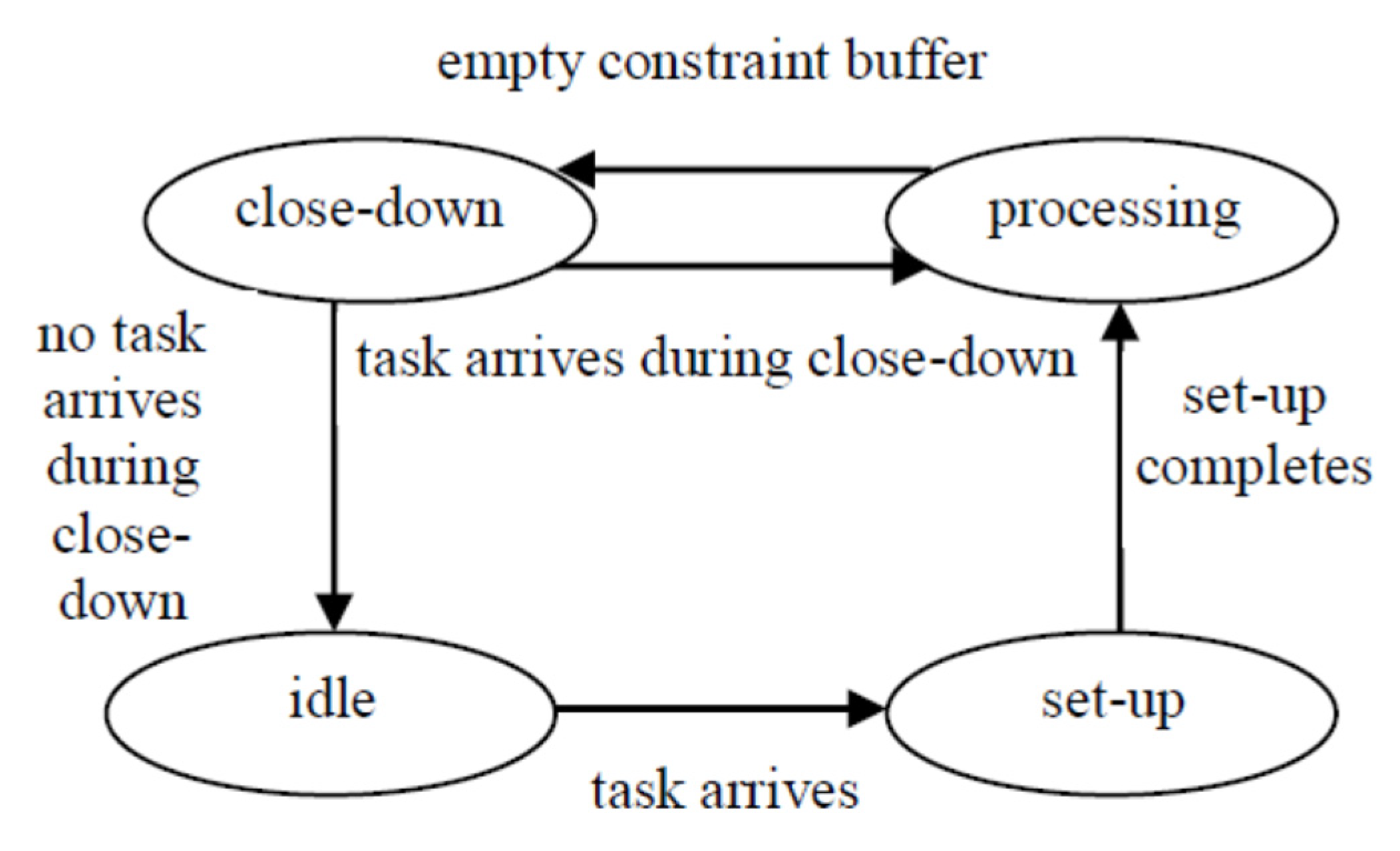
The sojourn time μ_n of task n = 1 … N depends on flow type, serial, parallel and serial–parallel. The transitions among the shutdown, setup and processing times are presented in Figure 1.

Schedule u is evaluated using four criteria in the optimization process:

• makespan function C(u):

$$\mathrm{C}\left(\mathrm{u}\right)=\max {\left[{\mathrm{t}}_{\mathrm{z},{\mathrm{V}}_{\mathrm{n}}}\right]}^{}$$

(7)

• Total delay of tasks T(u):

$$\mathrm{T}\left(\mathrm{u}\right)={\displaystyle \sum }_{\mathrm{n}=1}^{\mathrm{N}}\left[0,{\mathrm{D}}_{\mathrm{n}}\right],\mathrm{where}\{\begin{array}{c}0, \mathrm{if} {\mathrm{d}}_{\mathrm{n}}-{\mathrm{tz}}_{{\mathrm{V}}_{\mathrm{n}}}\le 0,\\ {\mathrm{D}}_{\mathrm{n}}, \mathrm{if} {\mathrm{d}}_{\mathrm{n}}-{\mathrm{tz}}_{{\mathrm{V}}_{\mathrm{n}}}>0.\end{array}$$

(8)

• Cost of tardiness or premature execution of tasks G (u):

$$\mathrm{G}\left(\mathrm{u}\right)={\displaystyle \sum }_{\mathrm{n}=1}^{\mathrm{N}}\left[{\mathrm{P}}_{\mathrm{n}}·{\mathrm{a}}_{\mathrm{n}},{\mathrm{D}}_{\mathrm{n}}·{\mathrm{b}}_{\mathrm{n}}\right],\mathrm{where}\{\begin{array}{c}{\mathrm{P}}_{\mathrm{n}}, \mathrm{if} {\mathrm{d}}_{\mathrm{n}}-{\mathrm{tz}}_{{\mathrm{V}}_{\mathrm{n}}}\le 0,\\ {\mathrm{D}}_{\mathrm{n}}, \mathrm{if} {\mathrm{d}}_{\mathrm{n}}-{\mathrm{tz}}_{{\mathrm{V}}_{\mathrm{n}}}>0.\end{array}$$

(9)

• Cost of energy consumption of machines E(u):

$$\mathrm{E}\left(\mathrm{u}\right)={\displaystyle \sum }_{\mathrm{l}=1}^{\mathrm{L}}\left[{\mathrm{Se}}_{\mathrm{l}}\cdot {\mathsf{\mu }}_{\mathrm{n},\mathrm{l}}+{\mathrm{Op}}_{\mathrm{l}}\cdot {\mathsf{\nu }}_{\mathrm{n},\mathrm{l}}+{\mathrm{Fa}}_{\mathrm{l}}\cdot {\pi }_{\mathrm{l}}+{\mathrm{St}}_{\mathrm{l}}\cdot {\varpi }_{\mathrm{l}}+{\mathrm{Cl}}_{\mathrm{l}}\cdot {\vartheta }_{\mathrm{l}}\right]{,}_{}$$

(10)

where tz_,vn is the completion time of operation v_n of task n, v_n = 1, …, V_n, n = 1, …, N, d_n is the deadline of task n, D_n is delay in completing task n, P_n is premature execution of task n, t_l,n is 1 or 0 depending on the state of the machine.

The matrix of delayed execution cost ${\mathrm{MA}}_{\mathrm{n}}={\left({\mathrm{a}}_{\mathrm{n}}\right)}_{\left(\mathrm{n}\right)\times \left(1\right)}$ represents the cost (penalty) for each day of delay for task n execution, ${\mathrm{a}}_{\mathrm{n}}\in \Re$ which may vary depending on the contract with the client task. The matrix of premature execution cost ${\mathrm{MB}}_{\mathrm{n}}={\left({\mathrm{b}}_{\mathrm{n}}\right)}_{\left(\mathrm{n}\right)\times \left(1\right)}$ represents the cost (penalty) for each day of premature execution for task n, ${\mathrm{b}}_{\mathrm{n}}\in \Re$ which may differ depending on the task.

The matrix of setup cost ${\mathrm{M}\mathsf{{\rm M}}}_{\mathrm{n},\mathrm{l}}={\left({\mathsf{\mu }}_{\mathrm{n},\mathrm{l}}\right)}_{\left(\mathrm{n}\right)\times \left(\mathrm{l}\right)}$ represents the energy cost used for setup, ${\mathsf{\mu }}_{\mathrm{n},\mathrm{l}}\in \Re$ which may differ depending on operation of task n executed on machine l. The matrix of operation cost ${\mathrm{M}\mathsf{{\rm N}}}_{\mathrm{n},\mathrm{l}}={\left({\mathsf{\nu }}_{\mathrm{n},\mathrm{l}}\right)}_{\left(\mathrm{n}\right)\times \left(\mathrm{l}\right)}$ represents the energy cost consumed for operation execution, ${\mathsf{\nu }}_{\mathrm{n},\mathrm{l}}\in \Re$ which may vary depending on the operation of task n executed on machine l.

The matrix of maintenance cost ${\mathrm{M}\Pi }_{\mathrm{l}}={\left({\pi }_{\mathrm{l}}\right)}_{\left(\mathrm{l}\right)\times \left(1\right)}$ represents the energy cost used to repair machine l. The matrix of standby cost ${\mathrm{M}\mathsf{{\rm Z}}}_{\mathrm{l}}={\left({\mathsf{\zeta }}_{\mathrm{l}}\right)}_{\left(\mathrm{l}\right)\times \left(1\right)}$ represents the energy cost used for the waiting time of machine l. The matrix of shutdown cost ${\mathrm{M}\mathsf{\Theta }}_{\mathrm{l}}={\left({\vartheta }_{\mathrm{l}}\right)}_{\left(\mathrm{l}\right)\times \left(1\right)}$ represents the energy cost used to shutdown machine l. In addition, ${\pi }_{\mathrm{j}},{\varpi }_{\mathrm{l}},{\vartheta }_{\mathrm{l}}\in \Re$, which may vary depending on machine l.

A set of promising solutions called Pareto-optimal set is a result of the multiple criteria optimization process using the Multi Objective Immune Algorithm (MOIA). The multi-criteria optimization problem is solved using the Weighted Aggregation Method (11). The best basic schedule is selected for the minimum value of the function:

$$\mathrm{FF}\left(\mathrm{u}\right)={\varpi }_1\cdot \mathrm{C}\left(\mathrm{u}\right)+{\varpi }_2\cdot \mathrm{T}\left(\mathrm{u}\right)+{\varpi }_3\cdot \mathrm{G}\left(\mathrm{u}\right)+{\varpi }_4\cdot \mathrm{E}\left(\mathrm{u}\right)$$

(11)

where: ϖ1,…, ϖ4 are the criterion weights defined by the decision maker, ϖ1, ϖ2, ϖ3, ϖ4 ∈[0,1] and the sum of the weights is equal to 1.

2.1. Multi Objective Immune Algorithm

The input data are divided into two groups; the first group is information about the production system, the second group contains the MOIA parameters:

• Number of evaluation criteria, type of evaluation criteria selected by a decision maker, number of tasks, number of machines, process routes, batch sizes, task completion times, operation times, setup times, shutdown times, failure times, the costs of energy consumption during machine operation, setup, shutdown and standby and the costs of delaying or premature completion of tasks;
• Subpopulation size for optimizing a single criterion, popsize, number of iterations (terminal condition) for endogenous population, endcond, number of iterations for exogenous population, exogcond, temperature parameter, temp, maximum number of genes mutated by hypermutation, numgenes, affinity threshold, affthres, suppression threshold, supthres.

2.1.1. Feasible Solution Encoding

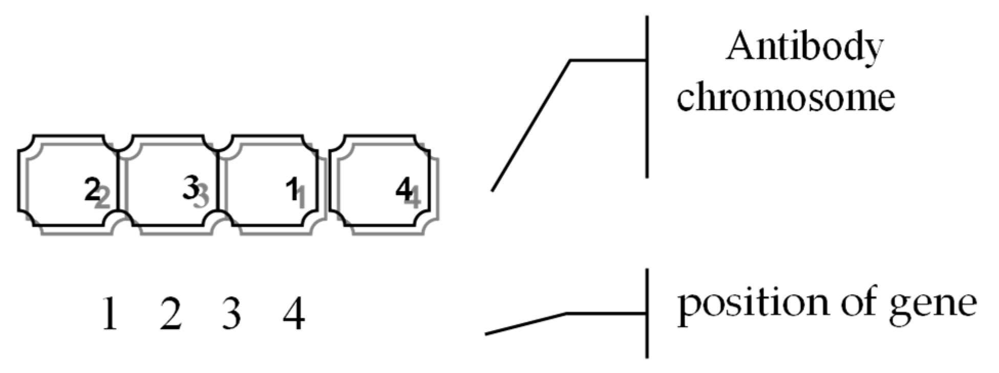
An antibody chromosome is represented by a sequence of decimal or binary task numbers (gene numbers). The length of the antibody chromosome is equal to a number of tasks performed in the flow shop system. The position of the gene corresponds to the priority indicator assigned to the task.

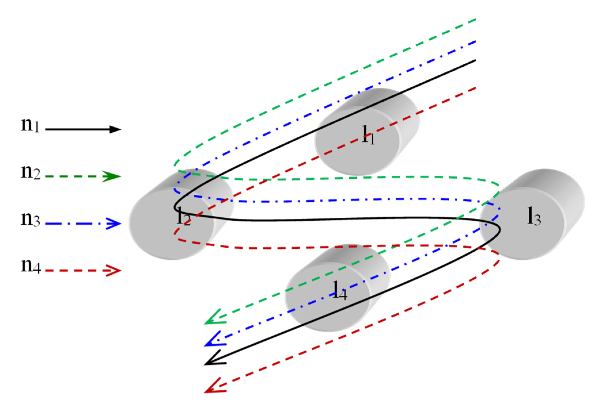
Consider the flow shop system defined by four production tasks, N = 4, and four machines, L = 4 (Figure 2). Job numbers are encoded in the DNA library (

Table 2. Genetic material in the DNA library for four tasks.

DNA Library				Generated Chromosomes	1	2	3	4
(n)					1	2	4	3
1	2	3	4		1	3	2	4
					4	3	2	1

). Antibodies are generated by random gene recombination from the DNA library. As a result, only active antibodies are generated, in other words, each chromosome contains all genes from the DNA library. The generation of unfeasible solutions is prevented by the permutational representation of genes in the chromosome.

Antibody decoding is started by reading a priority from left to right of the chromosome (Figure 3). First, task n = 2 is scheduled because it has the highest priority, then task n = 3 and n = 1 are scheduled, and finally task n = 4.

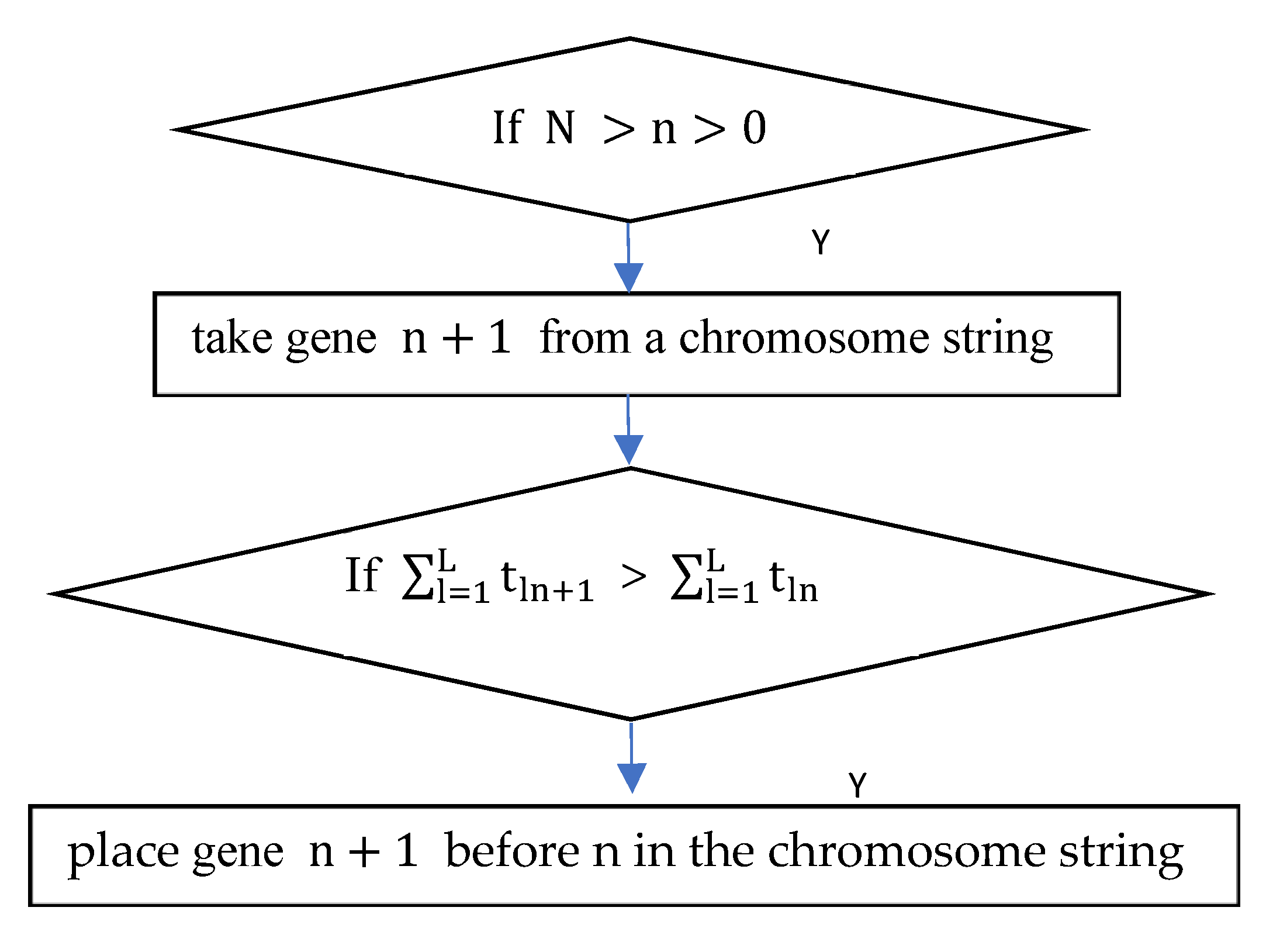
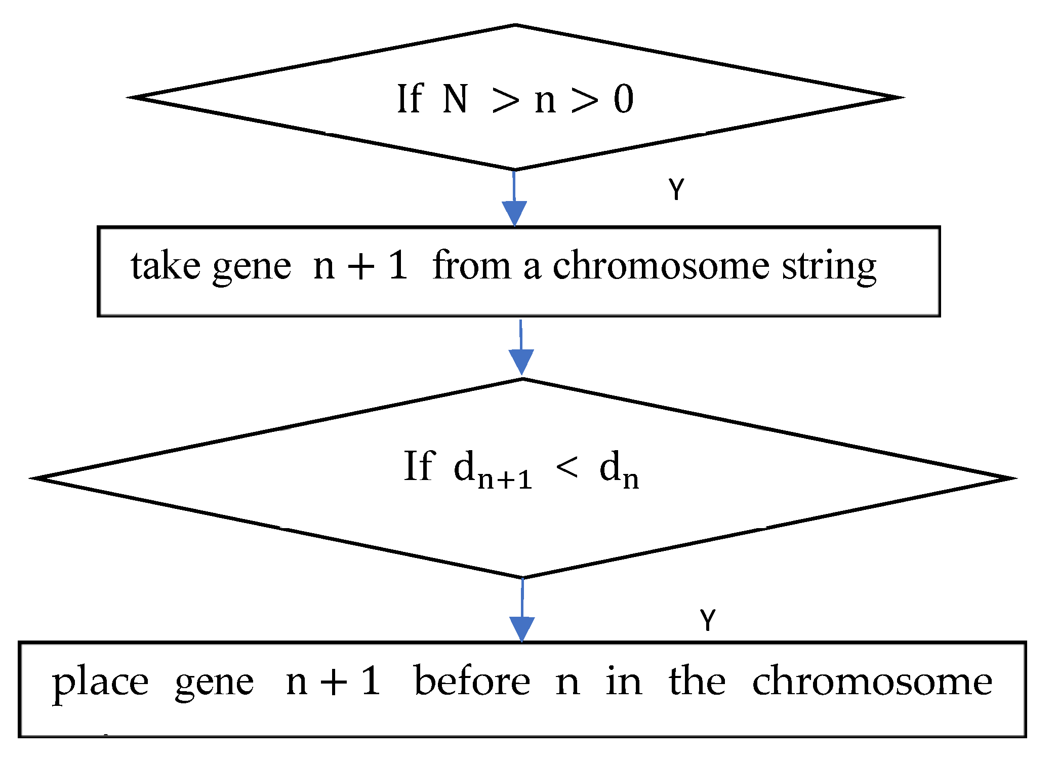
Better solutions can be obtained by starting the process of immunological optimization from points of interest in the solutions space. The solution space search process is continued for promising points (schedules) obtained with heuristics based on priority rules. When using the makespan criterion, the Least Processing Time (LPT) rule is proposed (Figure 4). The tasks that require the longest execution time are performed first.

In the EDD procedure, priority is given to the most urgent tasks with the earliest completion date (Figure 5). This procedure can be used if schedules are evaluated using the timeliness criteria.

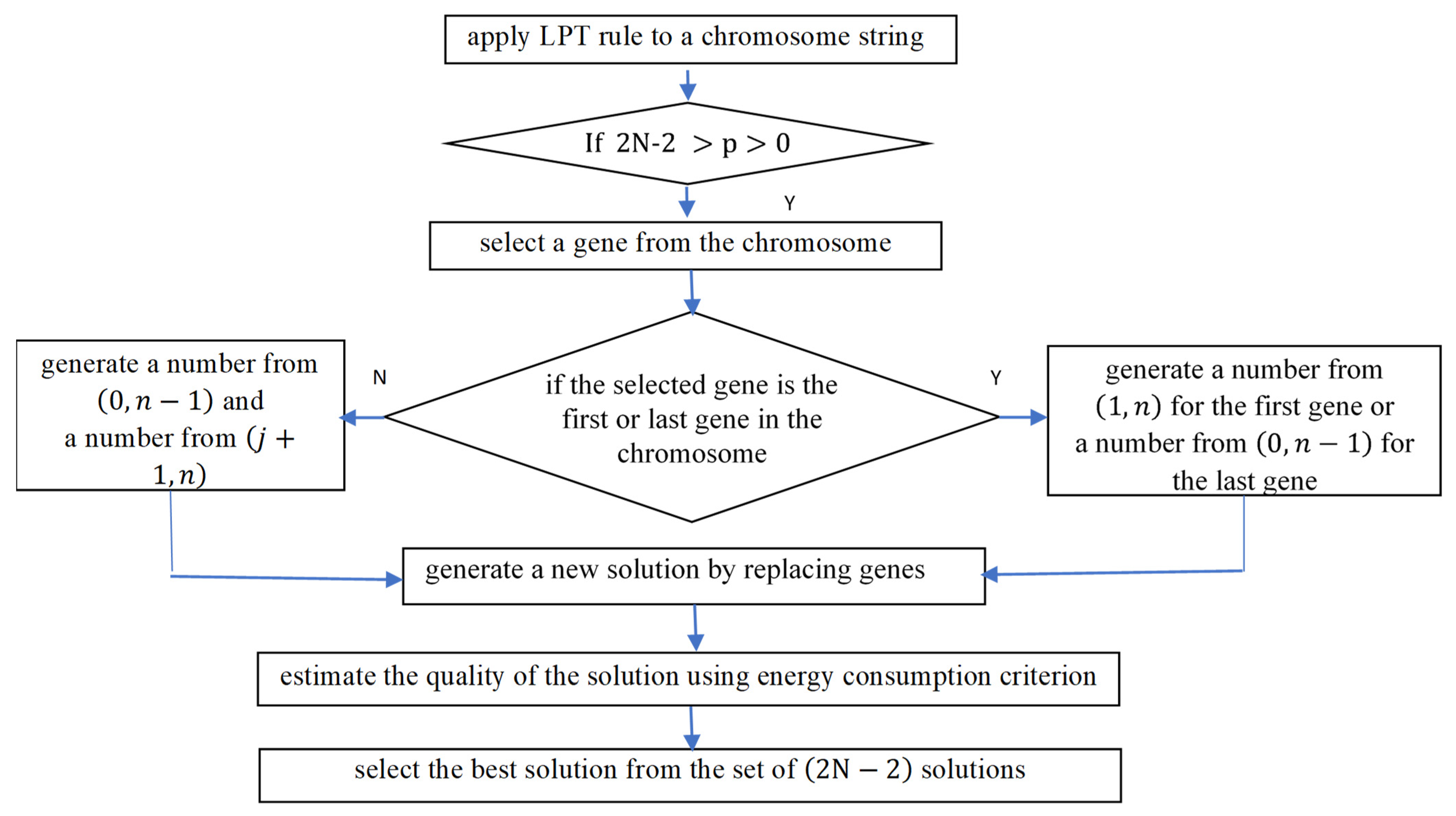
The random insertion perturbation scheme (RIPS) has been adapted to the task scheduling problem (Figure 6). This procedure is based on a local search for solution spaces around the solution generated using the LPT rule. The best neighborhood antibody is introduced into the initial population. The generated schedules are assessed according to the energy consumption criterion. In RIPS, a single number is randomly generated for the first and last jobs of the chromosome as they can only be shifted in one direction. The rest of the genes can be shifted in both directions.

2.1.2. The Maturation Process of Antibodies

In the immune system, antibodies undergo an affinity maturation process to better adopt to the pathogen, that is, to recognize and then destroy the pathogen. In the maturation process, crossover, mutation operators and hypermutation are used. The operators are used to increase the ability of the MOIA to search the solution space and achieve the optimal or near optimal schedule.

During the maturation process, the antibodies are copied and paired randomly to keep the population size constant. One offspring may be reproduced by each pair. A high reproductive probability is assumed to increase the emphasis on exploring the solution space. The following operators are used for the permutational representation of genes: Order Crossover (OX), Position-Based Crossover (PBX) and Linear Order Crossover (LOX).

In the OX procedure, a gene sequence is selected from the chromosome of the first parent [64,65]. The selected gene sequence is copied at the given positions to create the offspring chromosome. The selected genes are removed from the chromosome of the other parent. The genes required to complete the progeny chain remain. Going from left to right, the genes are copied in the order of the chromosome of the other parent (Figure 7).

The modified PBX [65] is proposed in order to generate a single progeny (Figure 8). Genes of the first chromosome are randomly selected. Offspring is made by copying the selected genes. The selected genes are removed from the chromosome of the other parent. As a result, genes are obtained that are the missing links in the offspring chromosome. Free spaces in the offspring chromosome are supplemented with missing genes following the order of the second chromosome from left to right.

In the modified LOX procedure [65], the set of genes from the first chromosome is selected randomly (Figure 9). Selected genes are removed from the first parent chromosome, leaving gaps. Free spaces are shifted from the extreme positions to the central part. In the offspring chromosome, empty space is filled by the remaining sequences of the genes of the second parent chromosome.

The following mutation operators can be used for the permutational representation of antibody chromosomes: Shift Mutation (SM), Insertion Mutation (IM), Displacement Mutation (DM) and Reciprocal Exchange Mutation (REM) [65]. The premature convergence of the MOIA to the local optimum is prevented by using the mutation operators to differentiate solutions.

In the SM procedure (Figure 10) an operation (gene) is randomly selected and then replaced with the previous gene. Assuming that the antibody chromosome consists of the number of N genes, a gene is randomly selected from the range $〈2,\mathrm{N}〉$.

In the IM procedure, the selected gene is placed at a new position in the offspring chromosome (Figure 11). Both the gene and its new position are selected from the range $〈1,\mathrm{N}〉$.

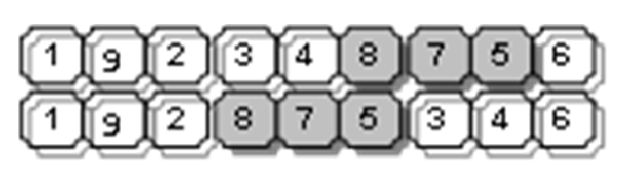
In the DM procedure, the gene substrings are randomly selected and placed in a random position in the range $〈1,\mathrm{N}〉$ (Figure 12). The probability of losing genetic material is higher using the DM procedure.

Two positions on the antibody chromosome are randomly selected by the REM procedure (Figure 13). The positions of genes are changed.

In the immune system, antibodies strongly stimulated by the pathogen undergo an intensified mutation process. The process of hypermutation involves modifying the antibody genes with varying frequency. In the hypermutation procedure, the better solutions remain unchanged, while the weak solutions are modified. In the hypermutation procedure, schedules are assessed using Equation (11) and the hypermutation index h is assigned to antibodies [66]. The antibodies are mutated at a different frequency depending on the hypermutation index h:

$$\mathrm{h}=\{\begin{array}{c}0, \mathrm{if} \mathrm{FF}{\left(\mathrm{u}\right)}^{\mathrm{r}}\in \langle \mathrm{FF}{\left(\mathrm{u}\right)}^{\mathrm{r},\min },\mathrm{FF}{\left(\mathrm{u}\right)}^{\mathrm{r},\min }+\Delta )\\ 1, \mathrm{if} \mathrm{FF}{\left(\mathrm{u}\right)}^{\mathrm{r}}\in \langle \mathrm{FF}{\left(\mathrm{u}\right)}^{\mathrm{r},\min }+\Delta ,\mathrm{FF}{\left(\mathrm{u}\right)}^{\mathrm{r},\max }-\Delta )\\ 2, \mathrm{if} \mathrm{FF}{\left(\mathrm{u}\right)}^{\mathrm{r}}\in \langle \mathrm{FF}{\left(\mathrm{u}\right)}^{\mathrm{r},\max }-\Delta ,\mathrm{FF}{\left(\mathrm{u}\right)}^{\mathrm{r},\max }\rangle \end{array}$$

(12)

$${\Delta }_{}=\left(\mathrm{FF}{\left(\mathrm{u}\right)}^{\mathrm{r},\max }-\mathrm{FF}{\left(\mathrm{u}\right)}^{\mathrm{r},\min }\right)/3$$

(13)

where: u—antibody, FF(u)^r,min—antibody with the minimum value of the fitness function (11) in generation r; FF(u)^r,max—antibody with the maximum value of the fitness function (11) in generation r; $\Delta$—threshold of the hypermutation index.

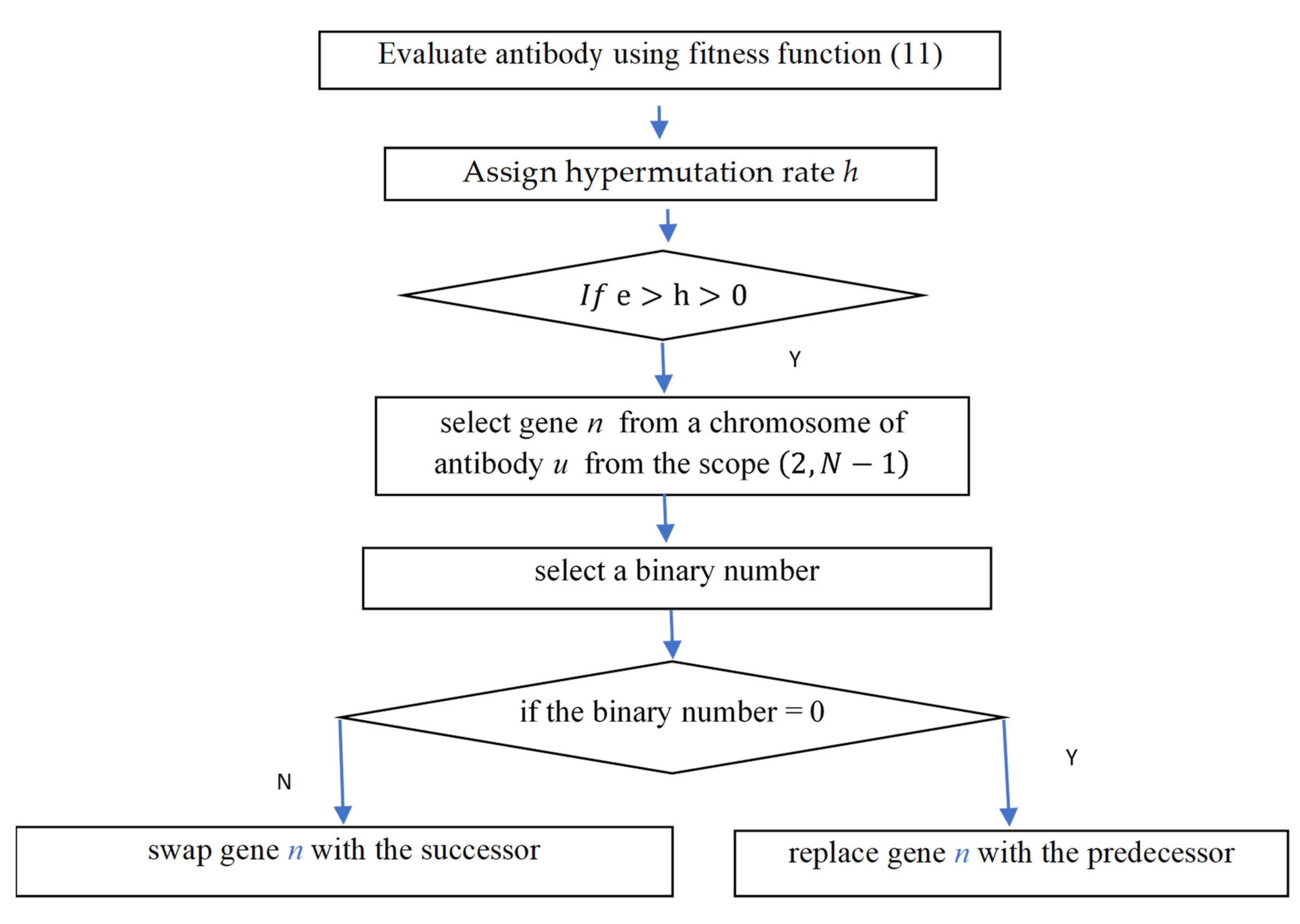
The hypermutation index h = 0 is assigned to the best antibodies that remain unchanged. H = 2 is assigned to the worst antibodies. For h = 2, the mutation procedure is performed twice. In the mutation procedure, gene n is selected from the range $〈2,\mathrm{N}〉-1$ and replaced with adjacent genes. The direction of the shift of gene n is also selected (Figure 14).

2.1.3. Control Parameters of the MOIA

The likelihood of failure when challenged with a new pathogen is increased in the case of a small number of different antibodies. A small number of different solutions make it difficult to escape from the path to the local optima. The diversity and quality of the antibodies can be controlled by mechanisms based on the temperature threshold, stimulation threshold and suppression threshold. In the multi-criteria search space, the search direction is selected using the mechanism based on the temperature threshold in order to increase the chances of obtaining antibodies recognizing the pathogen. The diversity of antibodies is controlled by mechanisms based on stimulation and suppression thresholds to prevent premature convergence of solutions to the local optimum.

In the immune system, the pathogen is only destroyed by the collective power of many antibodies. If the diversity of antibodies is insufficient, the effectiveness of the immune system′s response to the pathogen is reduced. Antibodies that recognize the pathogen are solutions in the neighborhood. A wide variety of solutions is maintained in the neighborhood reduction strategy. Similar or identical solutions are possible, but in a limited number.

Similar antibodies are identified in the stimulation mechanism. Let antibody u_k belong to neighborhood NG(u_k). The necessary condition of membership of antibody u_k+1 to neighborhood NG(u_k) is (14). The similarity of two solutions is determined by an affinity threshold value (affthres). The higher the affthres is, the longer Hamming distance between two antibodies can be, and two antibodies u_k and u_k+1 are classified to be similar (Equation (14)).

$${\mathrm{u}}_{\mathrm{k}+1}\in \mathrm{NG}\left({\mathrm{u}}_{\mathrm{k}}\right)\Rightarrow \left|{\mathrm{u}}_{\mathrm{k}+1},{\mathrm{u}}_{\mathrm{k}}\right|<\mathrm{affthres}$$

(14)

The affinity threshold depends on the size of the scheduling problem—the number of production jobs. The greater the number of production tasks, the greater the distance between the best and worst solutions. The affinity between two antibodies u_k and u_k+1 is measured using Hamming distance HD (15). The HD is computed as a number of positions whose bits b are different for two antibodies:

$$\mathrm{HD}\left|{\mathrm{u}}_{\mathrm{k}+1},{\mathrm{u}}_{\mathrm{k}}\right|={\displaystyle \sum }_{\mathrm{b}=0}^{\mathrm{B}}\left({\mathrm{u}}_{\mathrm{k}+1}^{\mathrm{b}}-{\mathrm{u}}_{\mathrm{k}}^{\mathrm{b}}\right)$$

(15)

A modified Hamming distance is applied in Equation (16). The modification is due to the chromosome coding method where each gene encodes a task number as a bit substring. Let q be the length of the substring s for which the compared bits are complementary, q ≥ 2. The sum of the complementary bits is increased by the length of each substring 2^q giving the degree of affinity (Equation (15)):

$$\mathrm{mHD}\left|{\mathrm{u}}_{\mathrm{k}+1},{\mathrm{u}}_{\mathrm{k}}\right|=\mathrm{HD}+{\wedge }_{\mathrm{s}}{{\displaystyle \sum }}_{\mathrm{b}=0}^{\mathrm{q}}{2}^{\mathrm{q}}$$

(16)

For chromosomes described by u_k+1 = [1110 0110 1011 0010] and u_k = [1100 1010 0111 0010] (Figure 15), the number of changes is equal to the number of tasks minus 1. Assuming the chromosomes are cyclic, the degree of affinity (Equation (16)) is computed for each gene change. Finally, the degree of affinity obtains the maximum value of mHD achieved for the first gene change. The affinity degree between antibodies u_k+1 and u_k is equal to 27 (

Table 3. The example of computing the degree of affinity between u_k+1 and u_k.

	uk+1	[1110 0110 1011 0010]
	uk	[1100 1010 0111 0010]
	HD	[0010 1100 1100 0000]
	mHD	=5 + 22 + 22 = 13
	uk+1	[1110 0110 1011 0010]
the first gene change	uk	[1010 0111 0010 1100]
	HD	[0100 0001 1001 1110]
	mHD	=7 + 22 + 24 = 27
	uk+1	[1110 0110 1011 0010]
the second gene change	uk	[0111 0010 1100 1010]
	HD	[1001 0100 0111 1000]
	mHD	=7 + 24 = 23
	uk+1	[1110 0110 1011 0010]
the third gene change	uk	[0010 1100 1010 0111]
	HD	[1100 1010 0001 0101]
	mHD	=7 + 22 = 11

).

The coefficient of antibody stimulation stimthres by other solutions is computed using (17):

$${\mathrm{stimthres}}_{\mathrm{k}}={\mathrm{stimthres}}_{\mathrm{k}}+1 \mathrm{if} \left|{\mathrm{u}}_{\mathrm{k}},{\mathrm{u}}_{\mathrm{k}+1}\right|<\mathrm{affthres}$$

(17)

In the suppression process, solution u_k is removed if stimthres is greater than a predefined value of the suppression threshold supthres. The balance between the diversity and quality of solutions is maintained using stimulation and suppression mechanisms.

2.1.4. The Multi Objective Immune Algorithm

In the MOIA, the pathogen is represented by the affinity function (Equation (11)) and the antibodies are represented by the schedules obtained for the flow shop problem. The artificial immune system has two stages: exogenous and endogenous activation. Exogenous activation is stimulated by the temperature parameter in the presence of the pathogen, which drives the defense response of the immune system. This phenomenon is used to obtain a promising search direction (vector of criteria weights) in the space of multi-criteria solutions.

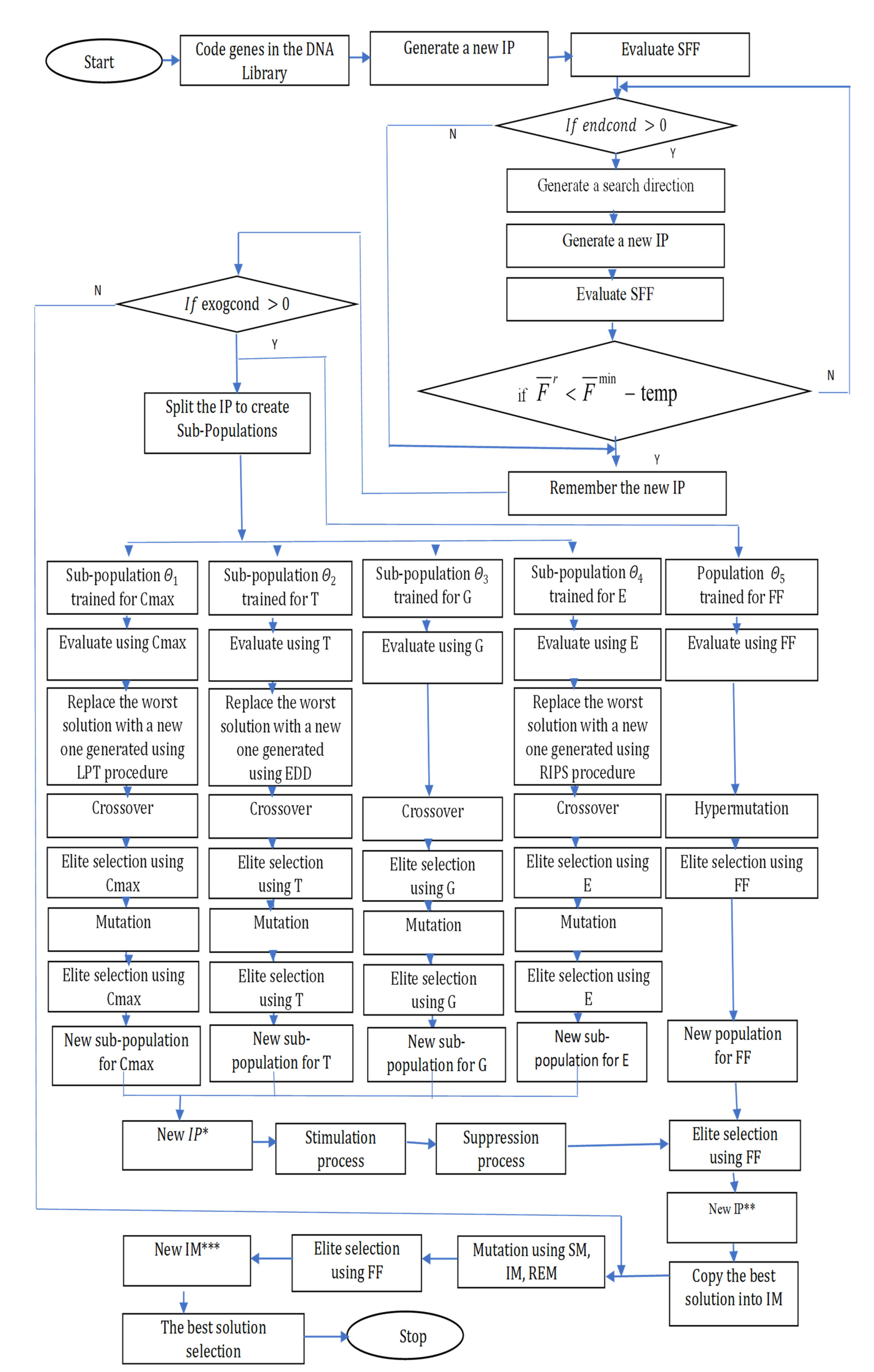
Endogenous activation includes the processes of antibody maturation, stimulation, and suppression. These phenomena are used to obtain promising solutions (schedules) in the immune memory (in the first immune response). Solutions are improved in the process of the second immune response due to the presence of the same or a similar pathogen. Steps of the MOIA are presented in Figure 15.

In step 1, the DNA library is encoded. In step 2, the process of generating antibodies is started by a random selection of genes from the DNA Library.

In step 3, the best vector of criteria weights is found. A promising direction of the search is the vector of weights for which the best initial population is obtained. The criteria weight vectors are selected randomly. The population mean quality (Equation (18)) is calculated using the scalar fitness function SFF (Equation (19)) and the selected weight vector. Equation (20) is verified in each generation of the endogenous activation for the promising weight vector selection. The advantage of searching for the best weight vector is the reduction of the computation time. Step 3 is omitted if the decision maker prioritizes the criteria (a constant vector of weights).

$${\overline{\mathrm{F}}}^{\mathrm{r}}=\frac{{{\displaystyle \sum }}_{\mathrm{k}=1}^{\mathrm{K}} \mathrm{SFF}{\left({\mathrm{u}}_{\mathrm{k}}\right)}^{\mathrm{r}}}{\mathrm{K}}$$

(18)

$$\mathrm{SFF}{\left(\mathrm{u}\right)}^{\mathrm{r}}={\varpi }_1\cdot \frac{\mathrm{C}{\left(\mathrm{u}\right)}^{\mathrm{r}}}{\mathrm{C}{\left({\mathrm{u}}^{*}\right)}^{\mathrm{r}}}+{\varpi }_2\cdot \frac{\mathrm{T}{\left(\mathrm{u}\right)}^{\mathrm{r}}}{\mathrm{T}{\left({\mathrm{u}}^{*}\right)}^{\mathrm{r}}}+{\varpi }_3\cdot \frac{\mathrm{G}{\left(\mathrm{u}\right)}^{\mathrm{r}}}{\mathrm{G}{\left({\mathrm{u}}^{*}\right)}^{\mathrm{r}}}+{\varpi }_4\cdot \frac{\mathrm{E}{\left(\mathrm{u}\right)}^{\mathrm{r}}}{\mathrm{E}{\left({\mathrm{u}}^{*}\right)}^{\mathrm{r}}},$$

(19)

$${\overline{\mathrm{F}}}^{\mathrm{r}}<{\overline{\mathrm{F}}}^{\mathrm{mintemp}}$$

(20)

where: u_k—antibody k, k = (1,2, …, K), ${\overline{\mathrm{F}}}^{\mathrm{r}}$—average quality of population r, ${\overline{\mathrm{F}}}^{\min }$—minimum value achieved for $\overline{\mathrm{F}}$.

In step 4, the initial population IP is divided into four sub-populations, Θ_1…Θ₄. Heuristic procedures are used to supply three sub-populations: the LPT, EDD and RIPS. The initial population (IP) is also copied to create sub-population Θ₅. In each sub-population, antibodies are decoded into schedules and evaluated using the single criterion (Equations (7)–(10)) for Θ_1…Θ₄, respectively and Equation (11) for Θ₅. Antibodies are selected randomly to create a matching pool in each sub-population. In sub-populations Θ_1…Θ₄, Position-Based Crossover is applied. Next, the elite selection procedure is carried out. Better individuals undergo Insertion Mutation and also the elite selection procedure is performed. All chromosomes undergo the maturation process. The hypermutation operator is used for generating a new offspring in sub-population Θ₅. Next, the elite selection procedure is carried out in the process of antibodies’ maturation in sub-population Θ₅.

In step 6, after combining sub-populations Θ_1…Θ₄ into a new initial population, similar antibodies are identified. Antibody u_k+1 belongs to the N(u_k) if the affthres between u_k and u_k+1 is less than or equal to stimthres.

The neighborhood reduction is performed in step 7. A number of similar antibodies belonging to the N(u_k) are controlled. In the suppression process, solution u_k+1 is removed from neighborhood N(u_k) if stimthres is greater than a predefined value of supthres.

The elite selection is carried out between two sub-populations: IP* and a new population for FF to create a new IP**.

The best solution is copied into the immune memory (IM) in each generation. In the secondary immune response, the neighborhoods of the memorized solutions are searched for better local solutions. The following mutation operators are used for a local search: SM, IM, REM. The fitness function (Equation (11)) is used for the selection pressure. The best solution from the memory, is the optimal or near to Pareto optimal solution, for the search direction achieved in step 3 or predefined by the decision maker.

3. Results and Detailed Discussions

Computer simulations were run for input buffer sizes equal to 10, 11, 12, 13, 14 and 15. Six simulation experiments were performed for each of the input data of the flow shop system. The production system consisted of 10 machines with given costs for energy consumption for operation, setup, shutdown and standby. Routes of production tasks were predefined. Production task completion dates and a penalty for delays or premature completion were also randomly assumed. Priority of objective function for makespan function C(u) equaled 0.3, total delay of tasks T(u) equaled 0.2, cost of tardiness or premature execution of tasks G(u) equaled 0.2 and cost of energy consumption of machines E(u) equaled 0.3. Data on process routes were based on previous research [56,57]. Deadlines of the processes were randomly selected.

Computer simulations were performed with the following MOIA input parameters: population size for the multi-criteria optimization problem (popsize) equaled 40, number of iterations for the endogenous population (endcond) equaled 10, number of iterations for the exogenous population (exogcond) equaled 4, maximum number of genes mutated by the hypermutation process (numgenes) equaled 2, affinity threshold (affthres) equaled 50, suppression threshold (supthres) equaled 3.

The observation and the analysis of sensitivity of the process, counting successive successfully processed tasks, to changing “input” parameters of the system, such as in-put buffer size n, setup times α, and shutdown times β, may provide useful information for optimization of the flow shop operation. The observation and the analysis of sensitivity of the process was performed for the types of flow: serial, parallel and serial–parallel.

3.1. The Influence of Interarrival Time on Criteria for the Serial-Parall Flow

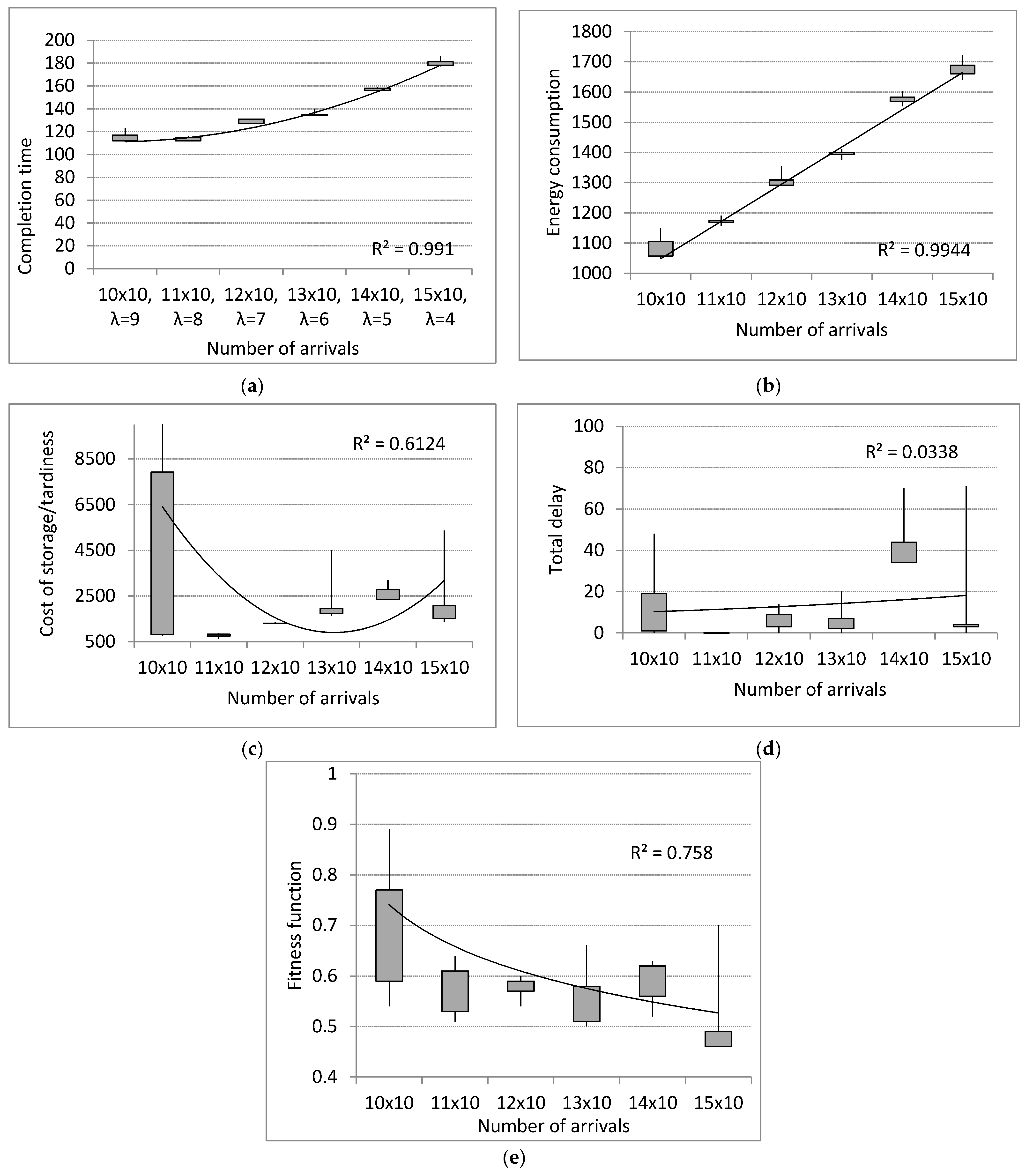
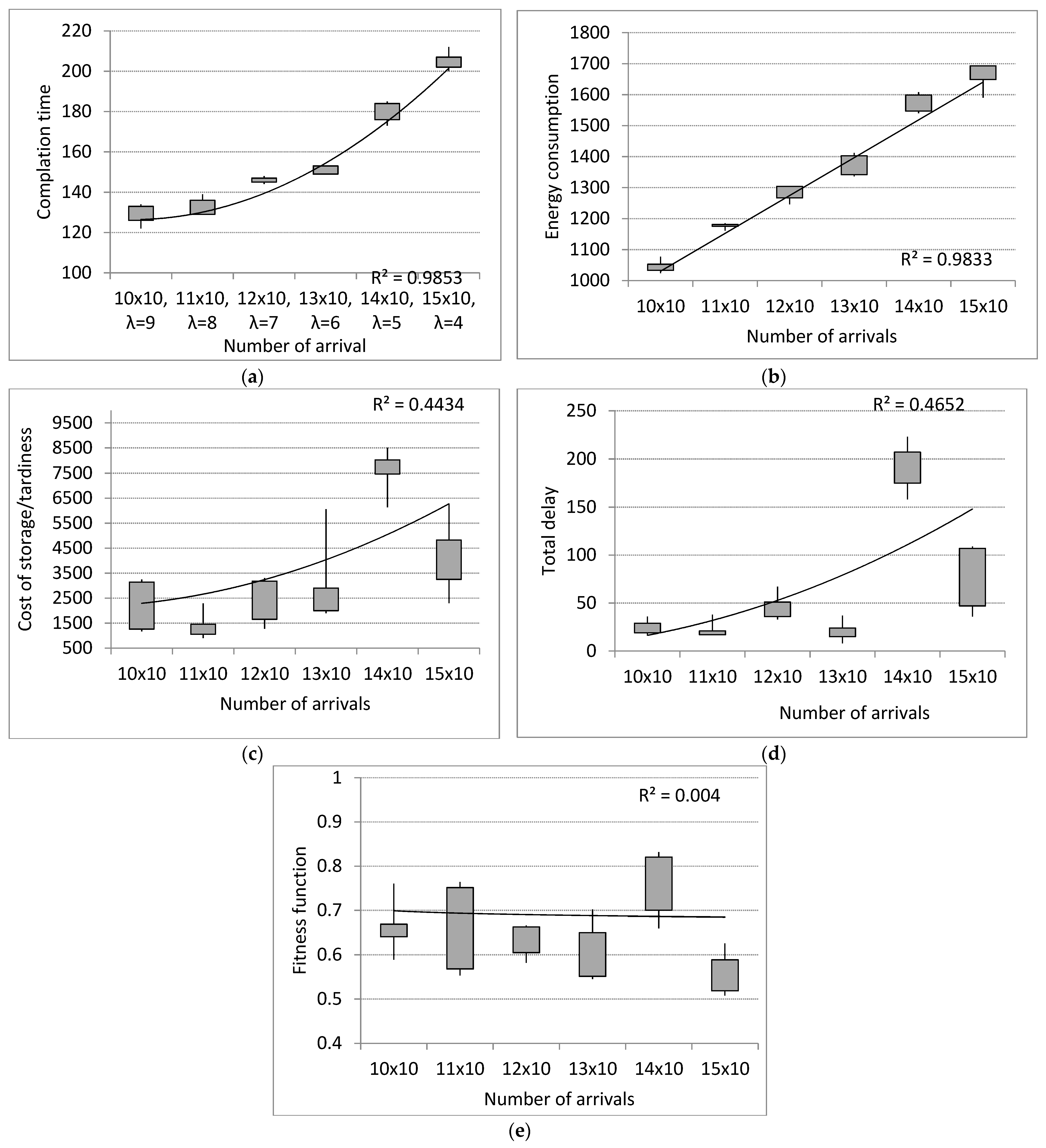
First, we investigated the effect of $\mathsf{\lambda }$ on the makespan before the fixed time epoch, T. Let us observe this characteristic after T = 250 (min), taking predefined values of processing times $\mathsf{\mu }$, setup times $\mathsf{\alpha }$, and shutdown times $\mathsf{\beta }$. Computer simulations were run for six different values of $\mathsf{\lambda }$ of two successive tasks, namely {9, 8, 7, 6, 5, 4} (min) and maximum system capacity N = 15. The results of the experiment are visualized in Figure 16. As one can observe, as $\mathsf{\lambda }$ increases the arrival intensity decreases. In addition, a slight change in the number of incoming tasks increases the makespan criterion more and more for the serial–parallel flow (Figure 16a). The cost of energy consumption increases with the number of orders accepted for execution (Figure 16b). The tardiness or premature execution criterion increases with the number of tasks from 10 to 14. The cost of tardiness or premature execution is reduced for tasks from 10 to 13 (Figure 16c). These phenomena can be explained by the stochastic nature of the immune algorithm. Each simulation increases the chance of getting a better solution. For each scheduling problem, timely schedules are achieved except 14 × 10 (Figure 16d). Timeline criteria should be prioritized to increase the likelihood of achieving non-delayed schedules. Scalar fitness function (Equation (19)) decreases with the increasing number of incoming tasks (Figure 16e). The SFF depends on the worst solutions achieved by the MOIA. The decreasing SFF value means that the worst quality solution improves with the increase in the number of incoming orders.

3.2. The Influence of Setup Times on Criteria for the Problem 15 × 10 and the Serial–Parallel Flow

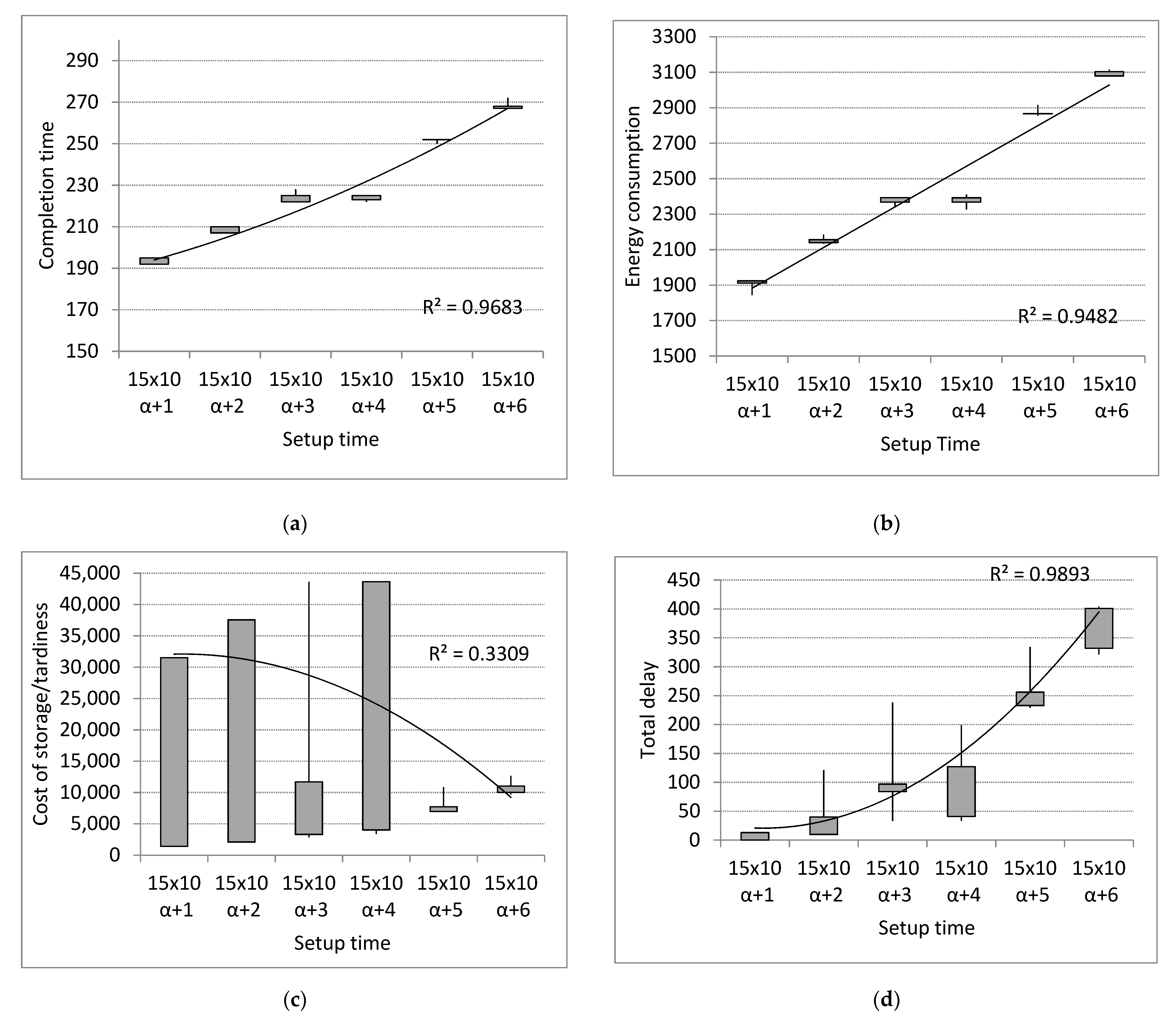
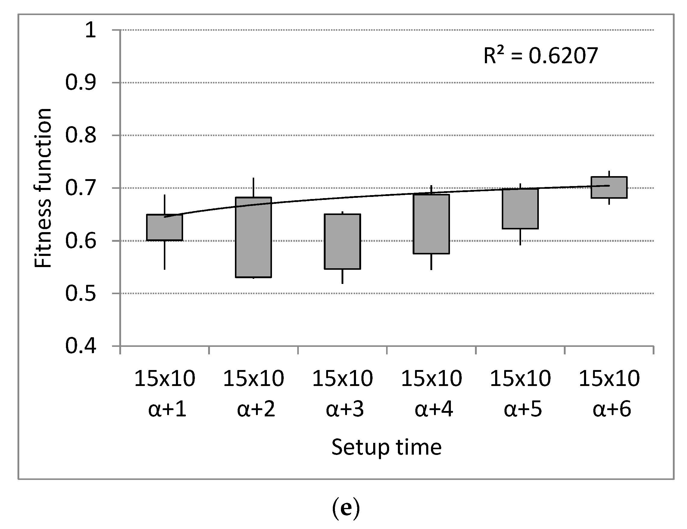
Let us investigate the impact of an increase of setup times α on criteria: makespan, total delay of tasks, cost of tardiness or premature execution of tasks, cost of energy consumption of machines for the flow shop system 15 × 10. Take T = 250 (min), N = 15, and observe the system for six different increases of α, namely α + 1, α + 2, α + 3, α + 4, α + 5 and α + 6 (min). The makespan criterion increases with increasing α (Figure 17a). The cost of energy consumption increases with setup times (Figure 17b). The interesting phenomena concern α + 3 and α + 4, where the increased setup times do not increase the energy consumption cost. This proves that the MOIA is efficient in achieving cost-effective schedules. The tardiness or premature execution criterion increases with α (Figure 17c). The cost of tardiness or premature execution is strongly related to the total delay of tasks (Figure 17d). Non-delayed schedules are only achieved when increasing setup times with 1 (Figure 17d). Scalar fitness function (Equation (19)) increases with setup times (Figure 17e).

3.3. The Influence of Shutdown Times on Criteria for the Problem 15 × 10 and the Serial–Parallel Flow

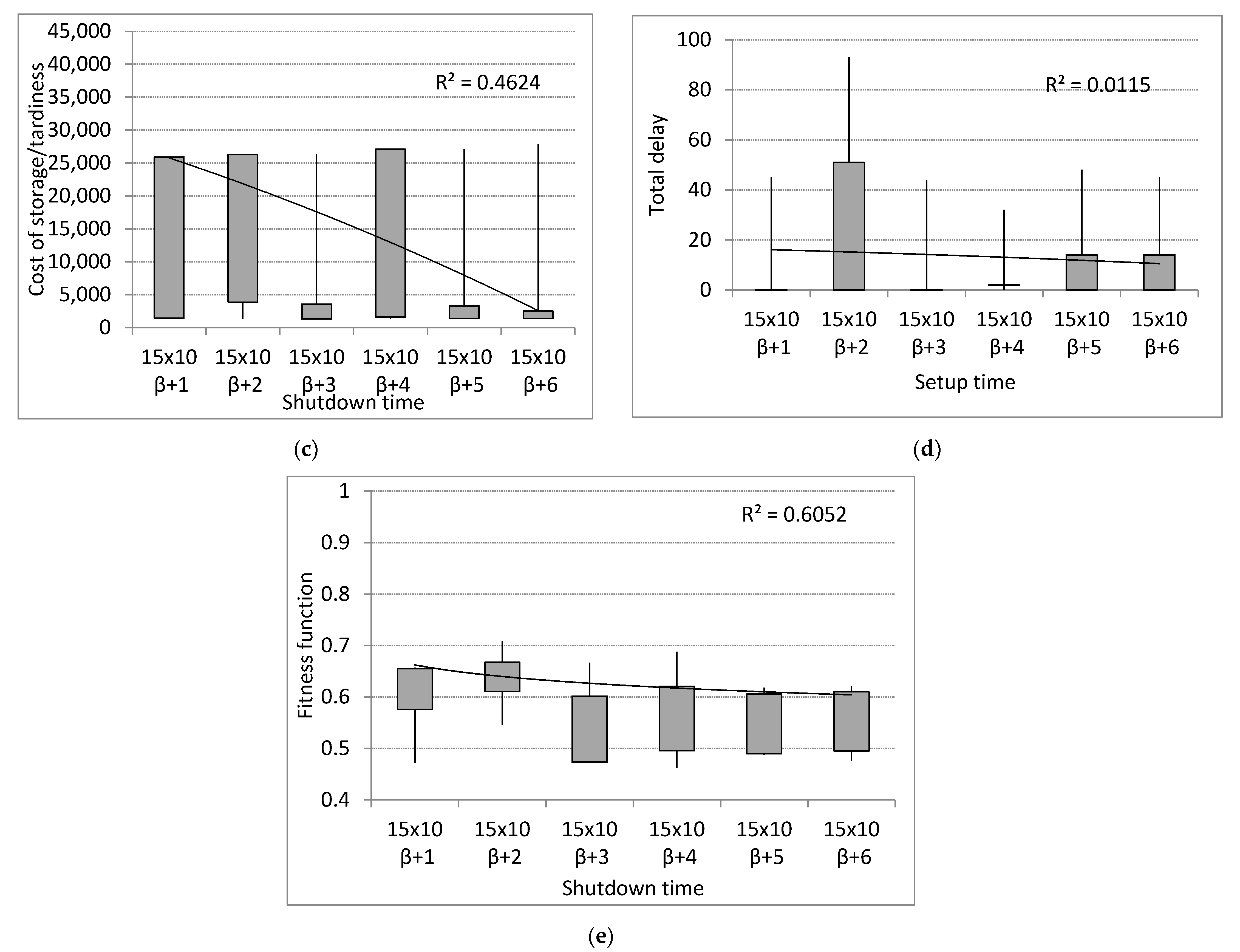
Let us examine the impact of increasing shutdown times β on the criteria: makespan, total delay of tasks, cost of tardiness or premature execution of tasks, cost of energy consumption of machines for the flow shop system 15 × 10. Take T = 250 (min), maximum size of the buffer N = 15 and observe the system for six different increments of β, namely β + 1, β + 2, β + 3, β + 4, β + 5 and β + 6 (min). As can be seen, any increase in β has very little effect on the makespan criterion (Figure 18a). The cost of energy consumption increases with shutdown times (Figure 18b). Interesting phenomena is for {β + 2, β + 3} and {β + 4, β + 5}, where the extension of shutdown times does not increase the cost of energy consumption. The MOIA achieves the same cost-effective schedules, even with increased shutdown times. The measurement of delay or premature execution does not increase with β (Figure 18c), taking into account the best achieved schedules. Non-delayed schedules are achieved for all extensions of downtime (Figure 18d). The scalar efficiency function (Equation (19)) decreases with increasing downtime (Figure 18e). These phenomena demonstrate MOIA’s ability to achieve profitable schedules.

3.4. The influence of Interarrival Time on Criteria for the Serial Flow

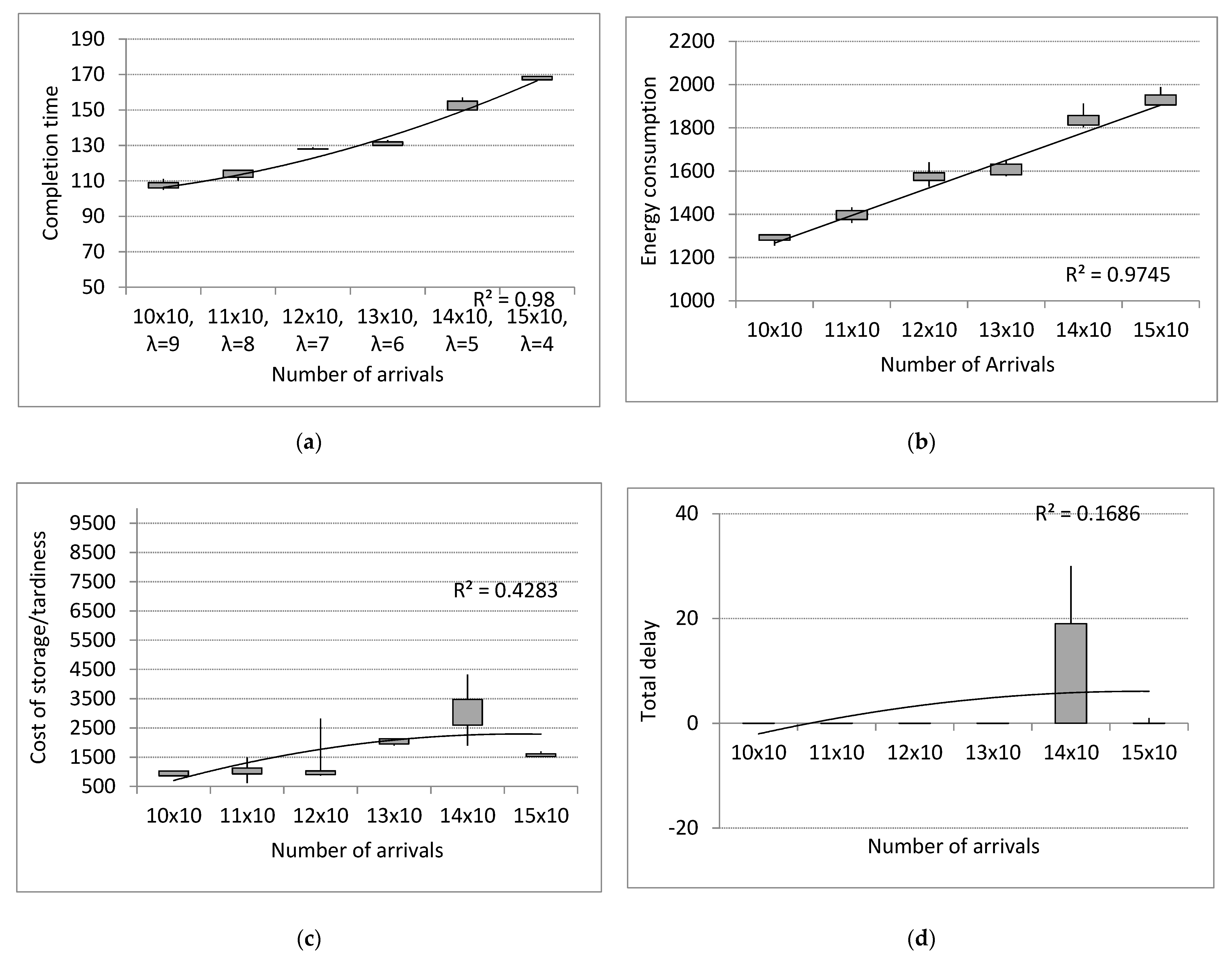
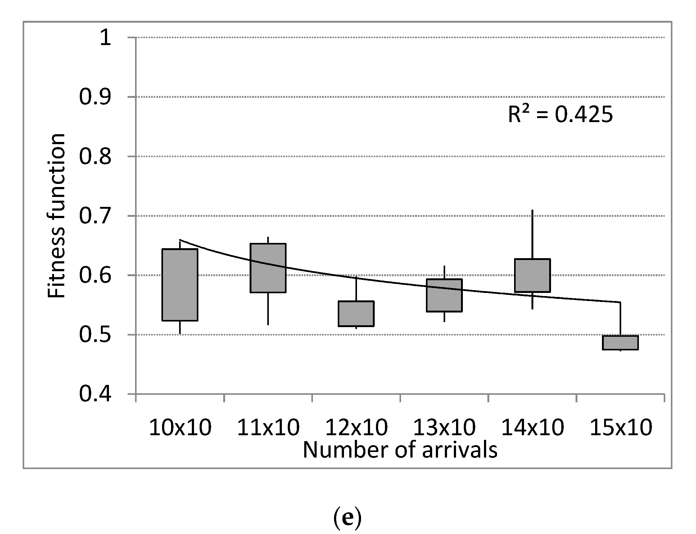
Here, the effect of different values of $\mathsf{\lambda }$ of two successive tasks on performance and cost-effective criteria for the serial flow of a batch accepted for execution is examined. Let us observe this characteristic after T = 250 (min), assuming predefined values for processing times $\mathsf{\mu }$, setup times $\mathsf{\alpha }$, and shutdown times $\mathsf{\beta }$. Computer simulations were performed for six different values of $\mathsf{\lambda }$, namely {9, 8, 7, 6, 5, 4} (min) and the maximum system capacity N = 15. The results of the experiment are presented in Figure 19. It can also be noted that a slight change in the number of incoming tasks increases the makespan criterion more and more for the serial flow (Figure 19a). The cost of energy consumption increases with the number of orders accepted for execution (Figure 19b). The tardiness or premature execution measurement increases with the number of tasks from 11 to 14. The cost of tardiness or premature execution decreases for 15 tasks (Figure 19c). The cost of tardiness or premature execution is strongly related to the total delay criterion. Schedules are unfeasible because tasks are delayed for each scheduling problem (Figure 19d). A decreasing SFF value means that the worst quality solution improves with an increase in the number of incoming orders (Figure 19e).

3.5. The Influence of Interarrival Time on Criteria for the Parallel Flow

Here, the effect of different values of $\mathsf{\lambda }$ of two successive tasks on performance and cost-effective criteria for the parallel flow in batch production is examined. Let us observe this characteristic after T = 250 (min), assuming predefined values of processing times $\mathsf{\mu }$, setup times $\mathsf{\alpha }$, shutdown times $\mathsf{\beta }$. Computer simulations were performed for six different values of $\mathsf{\lambda }$, namely {9, 8, 7, 6, 5, 4} (min) and the maximum system capacity N = 15. The results of the experiment are presented in Figure 20. In addition, one can note that a slight change in the number of incoming tasks increases the makespan criterion more and more for the parallel flow (Figure 20a). The cost of energy consumption increases with the number of orders accepted for execution (Figure 20b). The same cost-effective schedules are achieved for $\mathsf{\lambda }=\left\{6,7\right\}$. Theoretically, the tardiness or premature execution measurement increases with the number of tasks executed in the production system (Figure 20c). However, the same quality schedules achieved for number of tasks n = {10,11,12} can be noticed. These phenomena also prove the ability of the MOIA to achieve cost-effective schedules. For each scheduling problem and parallel flow, timely schedules are achieved (Figure 20d). The decreasing value of the SFF together with the increase in the number of incoming tasks also demonstrates the ability of the MOIA to achieve good quality schedules (Figure 20e).

4. Summary Discussion of the Results

In Section 3, each experiment was discussed in detail for the sake of clarity of the paper. In this section is a summary of the discussion. Comparing the effect of different values of λ of two successive tasks on performance and cost-effective criteria for the parallel, serial and serial–parallel flow the following conclusions can be drawn:

• The parallel flow of arriving tasks achieves the minimum values of makespan criterion (range from 109 to 170 (min)) (compare Figure 16a, Figure 19a and Figure 20a). The serial flow of arriving tasks achieves the worst quality schedules (range from 122 to 210 (min)) (Figure 19a).
• The serial flow (Figure 19b) and serial-parallel flow (Figure 16b) of arriving tasks achieves minimum cost of energy consumption (in range from 1050 to 1700). The parallel flow of arriving tasks achieves the worst quality schedules (energy consumption cost in the range from 1280 to 1980 (min)) (Figure 20b).
• The parallel flow of arriving tasks achieves minimum values of the costs of tardiness or premature execution (Figure 20c).
• Parallel flow and serial–parallel flow of incoming tasks achieves schedules with tasks that are non-delayed (Figure 20d and Figure 16d). Giving a high priority to the total delay criterion in the vector of weights achieves schedules with tasks that are non-delayed also for the problem 14 × 10.
• The decreasing value of the SFF with the increase in the number of incoming tasks proves the ability of the MOIA to achieve good quality schedules (Figure 16e, Figure 19e and Figure 20e).
• Observation and sensitivity analysis of the process, counting successive successfully processed tasks, to changing “input” parameters of the system, such as input buffer size n, setup times α, and shutdown times β may provide useful information for optimization of the flow shop operation. For example, extending the shutdown times (by 1 to 6 min) has very little effect on makespan criterion for the serial-parallel flow (18a).

5. Conclusions

Growing awareness of energy efficiency and sustainable development leads to a constant focus on energy efficiency in production planning. In this paper, the flow shop system with energy consumption parameters, setup and shutdown activities was considered. In such flow shop systems, minimizing the schedule time (makespan) is tantamount to minimizing energy consumption, as energy consumption is proportional to machine power and processing time. However, the energy consumption is only one of many factors affecting the total manufacturing cost, and the costs of delay and storage are also important.

The computed results indicate that the proposed energy-efficient scheduling approach, and corresponding Multi Objective Immune Algorithms, can indeed optimize the decision target, effectively solving the problem. As the experiments show, the organization of the production flow has a large impact on energy consumption. The lowest level of energy consumption can be achieved with the serial–parallel flow, but with the need for additional storage buffers and a greater likelihood of delays.

In addition, the main contributions of this paper compared to related papers [32,33,34,35,36,37,38,39,40,41,42,43,44,45], are as follows:

• The multi-objective scheduling model has been developed that takes into account four objectives;
• The parameters for setup and shutdown with energy consumption were incorporated into the algorithm.

It should be noticed that, from the production manager’s point of view, the volatility of supply and demand and stock levels throughout the supply chain, as well as energy price changes, are important [9,10], and they will be the subject of future research. A preventive maintenance policy is also an important issue as machine failures and unplanned downtime severely disrupt production schedules [57].

For future work, the proposed algorithm will be tested in various planning environments such as the job shop and the open shop scheduling environment to verify its more general applicability.

References

- Menghi, R.; Papetti, A.; Germani, M.; Marconi, M. Energy efficiency of manufacturing systems: A review of energy assessment methods and tools. J. Clean. Prod. 2019, 240, 118276. [Google Scholar] [CrossRef]
- Renna, P.; Materi, S. A literature review of energy efficiency and sustainability in manufacturing systems. Appl. Sci. 2021, 11, 7366. [Google Scholar] [CrossRef]
- Bozek, A. Energy cost-efficient task positioning in manufacturing systems. Energies 2020, 13, 5034. [Google Scholar] [CrossRef]
- Chung, K.H.; Hur, D. Towards the design of P2P energy trading scheme based on optimal energy scheduling for prosumers. Energies 2020, 13, 5177. [Google Scholar] [CrossRef]
- Herenčić, L.; Ilak, P.; Rajšl, I. Effects of local electricity trading on power flows and voltage levels for different elasticities and prices. Energies 2019, 12, 4708. [Google Scholar] [CrossRef] [Green Version]
- Mihet-Popa, L.; Saponara, S. Power converters, electric drives and energy storage systems for electrified transportation and smart grid applications. Energies 2021, 14, 4142. [Google Scholar] [CrossRef]
- Sihag, N.; Sangwan, K.S. A systematic literature review on machine tool energy consumption. J. Clean. Prod. 2020, 275, 123125. [Google Scholar] [CrossRef]
- Garai, A.; Chowdhury, S.; Sarkar, B.; Roy, T.K. Cost-effective subsidy policy for growers and biofuels-plants in closed-loop supply chain of herbs and herbal medicines: An interactive bi-objective optimization in T-environment. Appl. Soft Comput. 2020, 100, 106949. [Google Scholar] [CrossRef]
- Bhuniya, S.; Pareek, S.; Sarkar, B.; Sett, B.K. A smart production process for the optimum energy consumption with maintenance policy under a supply chain management. Processes 2021, 9, 19. [Google Scholar] [CrossRef]
- Marinakis, V.; Koutsellis, T.; Nikas, A.; Doukas, H. Ai and data democratisation for intelligent energy management. Energies 2021, 14, 4341. [Google Scholar] [CrossRef]
- Vandana; Singh, S.R.; Yadav, D.; Sarkar, B.; Sarkar, M. Impact of energy and carbon emission of a supply chain management with two-level trade-credit policy. Energies 2021, 14, 1569. [Google Scholar] [CrossRef]
- Rocha, A.D.; Freitas, N.; Alemão, D.; Guedes, M.; Martins, R.; Barata, J. Event-Driven Interoperable Manufacturing Ecosystem for Energy Consumption Monitoring. Energies 2021, 14, 3620. [Google Scholar] [CrossRef]
- Fahad, M.; Shahid, A.; Manumachu, R.R.; Lastovetsky, A. A comparative study of methods for measurement of energy of computing. Energies 2019, 12, 2204. [Google Scholar] [CrossRef] [Green Version]
- Zhou, L.; Li, J.; Li, F.; Meng, Q.; Li, J.; Xu, X. Energy consumption model and energy efficiency of machine tools: A comprehensive literature review. J. Clean. Prod. 2016, 112, 3721–3734. [Google Scholar] [CrossRef]
- Grigor’ev, S.N.; Kuznetsov, A.P.; Volosova, M.A.; Koriath, H.J. Classification of metal-cutting machines by energy efficiency. Russ. Eng. Res. 2014, 34, 136–141. [Google Scholar] [CrossRef]
- Gahm, C.; Denz, F.; Dirr, M.; Tuma, A. Energy-efficient scheduling in manufacturing companies: A review and research framework. Eur. J. Oper. Res. 2016, 248, 744–757. [Google Scholar] [CrossRef]
- Gao, K.; Huang, Y.; Sadollah, A.; Wang, L. A review of energy-efficient scheduling in intelligent production systems. Complex Intell. Syst. 2019, 6, 237–249. [Google Scholar] [CrossRef] [Green Version]
- Nouiri, M.; Bekrar, A.; Trentesaux, D. An energy-efficient scheduling and rescheduling method for production and logistics systems. Int. J. Prod. Res. 2019, 58, 3263–3283. [Google Scholar] [CrossRef]
- De Courchelle, I.; Guérout, T.; Da Costa, G.; Monteil, T.; Labit, Y. Green energy efficient scheduling management. Simul. Model. Pract. Theory 2018, 93, 208–232. [Google Scholar] [CrossRef]
- Nouiri, M.; Trentesaux, D.; Bekrar, A. Towards energy efficient scheduling of manufacturing systems through collaboration between cyber physical production and energy systems. Energies 2019, 12, 4448. [Google Scholar] [CrossRef] [Green Version]
- Cui, W.; Li, L.; Lu, Z. Energy-efficient scheduling for sustainable manufacturing systems with renewable energy resources. Nav. Res. Logist. 2019, 66, 154–173. [Google Scholar] [CrossRef]
- Saddikuti, V.; Pesaru, V. NSGA Based Algorithm for Energy Efficient Scheduling in Cellular Manufacturing. Procedia Manuf. 2019, 39, 1002–1009. [Google Scholar] [CrossRef]
- Wang, S.; Liu, M.; Chu, F.; Chu, C. Bi-objective optimization of a single machine batch scheduling problem with energy cost consideration. J. Clean. Prod. 2016, 137, 1205–1215. [Google Scholar] [CrossRef] [Green Version]
- Jiang, Q.; Liao, X.; Zhang, R.; Lin, Q. Energy-Saving Production Scheduling in a Single-Machine Manufacturing System by Improved Particle Swarm Optimization. Math. Probl. Eng. 2020, 2020, 8870917. [Google Scholar] [CrossRef]
- Shrouf, F.; Ordieres-Meré, J.; García-Sánchez, A.; Ortega-Mier, M. Optimizing the production scheduling of a single machine to minimize total energy consumption costs. J. Clean. Prod. 2014, 67, 197–207. [Google Scholar] [CrossRef]
- Chen, L.; Wang, J.; Xu, X. An energy-efficient single machine scheduling problem with machine reliability constraints. Comput. Ind. Eng. 2019, 137, 106072. [Google Scholar] [CrossRef]
- Zhou, S.; Jin, M.; Du, N. Energy-efficient scheduling of a single batch processing machine with dynamic job arrival times. Energy 2020, 209, 118420. [Google Scholar] [CrossRef]
- Wang, G.; Li, X.; Gao, L.; Li, P. An effective multi-objective whale swarm algorithm for energy-efficient scheduling of distributed welding flow shop. Ann. Oper. Res. 2021, 297, 1–33. [Google Scholar] [CrossRef]
- Ho, M.H.; Hnaien, F.; Dugardin, F. Electricity cost minimisation for optimal makespan solution in flow shop scheduling under time-of-use tariffs. Int. J. Prod. Res. 2020, 59, 1041–1067. [Google Scholar] [CrossRef]
- Tang, D.; Dai, M.; Salido, M.A.; Giret, A. Energy-efficient dynamic scheduling for a flexible flow shop using an improved particle swarm optimization. Comput. Ind. 2016, 81, 82–95. [Google Scholar] [CrossRef]
- Wu, X.; Shen, X.; Cui, Q. Multi-objective flexible flow shop scheduling problem considering variable processing time due to renewable energy. Sustainbility 2018, 10, 841. [Google Scholar] [CrossRef] [Green Version]
- Yan, J.; Li, L.; Zhao, F.; Zhang, F.; Zhao, Q. A multi-level optimization approach for energy-efficient flexible flow shop scheduling. J. Clean. Prod. 2016, 137, 1543–1552. [Google Scholar] [CrossRef]
- Kong, L.; Wang, L.; Li, F.; Wang, G.; Fu, Y.; Liu, J. A New Sustainable Scheduling Method for Hybrid Flow-Shop Subject to the Characteristics of Parallel Machines. IEEE Access 2020, 8, 79998–80009. [Google Scholar] [CrossRef]
- Meng, L.; Zhang, C.; Shao, X.; Ren, Y.; Ren, C. Mathematical modelling and optimisation of energy-conscious hybrid flow shop scheduling problem with unrelated parallel machines. Int. J. Prod. Res. 2018, 57, 1119–1145. [Google Scholar] [CrossRef] [Green Version]
- Chen, J.; Wang, L.; Peng, Z. A collaborative optimization algorithm for energy-efficient multi-objective distributed no-idle flow-shop scheduling. Swarm Evol. Comput. 2019, 50. [Google Scholar] [CrossRef]
- Wang, G.; Li, X.; Gao, L.; Li, P. Energy-efficient distributed heterogeneous welding flow shop scheduling problem using a modified MOEA/D. Swarm Evol. Comput. 2021, 62, 100858. [Google Scholar] [CrossRef]
- Wu, X.; Che, A. Energy-efficient no-wait permutation flow shop scheduling by adaptive multi-objective variable neighborhood search. Omega 2019, 94, 102117. [Google Scholar] [CrossRef]
- Zhang, B.; Pan, Q.K.; Gao, L.; Meng, L.L.; Li, X.Y.; Peng, K.K. A Three-Stage Multiobjective Approach Based on Decomposition for an Energy-Efficient Hybrid Flow Shop Scheduling Problem. IEEE Trans. Syst. Man Cybern. Syst. 2019, 50, 4984–4999. [Google Scholar] [CrossRef]
- Wang, J.J.; Wang, L. A Knowledge-Based Cooperative Algorithm for Energy-Efficient Scheduling of Distributed Flow-Shop. IEEE Trans. Syst. Man Cybern. Syst. 2018, 50, 1805–1819. [Google Scholar] [CrossRef]
- Lu, C.; Gao, L.; Yi, J.; Li, X. Energy-Efficient Scheduling of Distributed Flow Shop with Heterogeneous Factories: A Real-World Case from Automobile Industry in China. IEEE Trans. Ind. Inform. 2020, 17, 6687–6696. [Google Scholar] [CrossRef]
- Zhou, R.; Lei, D.; Zhou, X. Multi-Objective Energy-Efficient Interval Scheduling in Hybrid Flow Shop Using Imperialist Competitive Algorithm. IEEE Access 2019, 7, 85029–85041. [Google Scholar] [CrossRef]
- Ebrahimi, A.; Jeon, H.W.; Lee, S.; Wang, C. Minimizing total energy cost and tardiness penalty for a scheduling-layout problem in a flexible job shop system: A comparison of four metaheuristic algorithms. Comput. Ind. Eng. 2020, 141, 106295. [Google Scholar] [CrossRef]
- Jiang, T.; Zhang, C.; Sun, Q.M. Green Job Shop Scheduling Problem with Discrete Whale Optimization Algorithm. IEEE Access 2019, 7, 43153–43166. [Google Scholar] [CrossRef]
- Yin, L.; Li, X.; Gao, L.; Lu, C.; Zhang, Z. Energy-efficient job shop scheduling problem with variable spindle speed using a novel multi-objective algorithm. Adv. Mech. Eng. 2017, 9. [Google Scholar] [CrossRef] [Green Version]
- Wang, H.; Jiang, Z.; Wang, Y.; Zhang, H.; Wang, Y. A two-stage optimization method for energy-saving flexible job-shop scheduling based on energy dynamic characterization. J. Clean. Prod. 2018, 188, 575–588. [Google Scholar] [CrossRef]
- Gong, X.; De Pessemier, T.; Martens, L.; Joseph, W. Energy- and labor-aware flexible job shop scheduling under dynamic electricity pricing: A many-objective optimization investigation. J. Clean. Prod. 2019, 209. [Google Scholar] [CrossRef] [Green Version]
- Mokhtari, H.; Hasani, A. An energy-efficient multi-objective optimization for flexible job-shop scheduling problem. Comput. Chem. Eng. 2018, 209, 1078–1094. [Google Scholar] [CrossRef]
- Mousavi, M.; Yap, H.J.; Musa, S.N.; Tahriri, F.; Md Dawal, S.Z. Multi-objective AGV scheduling in an FMS using a hybrid of genetic algorithm and particle swarm optimization. PLoS ONE 2017, 104, 339–352. [Google Scholar] [CrossRef] [PubMed] [Green Version]
- Yin, L.; Li, X.; Lu, C.; Gao, L. Energy-efficient scheduling problem using an effective hybrid multi-objective evolutionary algorithm. Sustainbility 2016, 8, 1268. [Google Scholar] [CrossRef] [Green Version]
- Utama, D.M.; Widodo, D.S. An energy-efficient flow shop scheduling using hybrid harris hawks optimization. Bull. Electr. Eng. Inform. 2021, 10, 1154–1163. [Google Scholar] [CrossRef]
- Gutowski, T.; Dahmus, J.; Thiriez, A. Electrical energy requirements for manufacturing processes. In Proceedings of the Proceedings of the 13th CIRP International Conference on Life Cycle Engineering, LCE 2006, Leuven, Belgium, 31 May–2 June 2006. [Google Scholar]
- Paprocka, I.; Kampa, A.; Gołda, G. The effects of a machine failure on the robustness of job shop systems-the predictive-reactive approach. Int. J. Mod. Manuf. Technol. 2019, 11, 72–79. Available online: https://ijmmt.ro/vol11no22019/11_Iwona_Paprocka.pdf (accessed on 8 August 2021).
- Paprocka, I. Evaluation of the effects of a machine failure on the robustness of a job shop system-proactive approaches. Sustain. 2018, 11, 65. [Google Scholar] [CrossRef] [Green Version]
- Shoeb, M. Implementation of Lean Manufacturing System for Successful Production System in Manufacturing Industries. Int. J. Eng. Res. Appl. 2017, 7, 41–46. [Google Scholar] [CrossRef]
- Fowler, J.W.; Mönch, L. A survey of scheduling with parallel batch (p-batch) processing. Eur. J. Oper. Res. 2021. [Google Scholar] [CrossRef]
- Paprocka, I.; Kempa, W.M.; Kalinowski, K.; Grabowik, C. A production scheduling model with maintenance. Adv. Mater. Res. 2014, 1036, 885–890. [Google Scholar] [CrossRef]
- Paprocka, I.; Urbanek, D. A numerical example of total production maintenance and robust scheduling application for a production system efficiency increasing. J. Mach. Eng. 2012, 12, 62–79. [Google Scholar]
- Paprocka, I. Total production maintenance and robust scheduling for a production system efficiency increasing. J. Mach. Eng. 2012, 12, 52–61. [Google Scholar]
- Barosz, P.; Gołda, G.; Kampa, A. Efficiency Analysis of Manufacturing Line with Industrial Robots and Human Operators. Appl. Sci. 2020, 10, 2862. [Google Scholar] [CrossRef] [Green Version]
- Kampa, A.; Gołda, G. Modelling and simulation method for production process automation in steel casting foundry. Arch. Foundry Eng. 2018. [Google Scholar] [CrossRef]
- Foit, K.; Gołda, G.; Kampa, A. Integration and evaluation of intra-logistics processes in flexible production systems based on oee metrics, with the use of computer modelling and simulation of agvs. Processes 2020, 8, 1648. [Google Scholar] [CrossRef]
- Kempa, W.M.; Paprocka, I. Analytical Solution for Time-Dependent Queue-Size Behavior in the Manufacturing Line with Finite Buffer Capacity and Machine Setup and Closedown Times. Appl. Mech. Mater. 2015, 809–810, 1360–1365. [Google Scholar] [CrossRef]
- Paprocka, I.; Kempa, W.M.; Krenczyk, D. Analysis of queue-size behaviour and throughput of a system with buffer controlled by a rope and production speed controlled by a drum. Int. J. Mod. Manuf. Technol. 2019, XI, 128–136. [Google Scholar]
- Liaw, C.F. Hybrid genetic algorithm for the open shop scheduling problem. Eur. J. Oper. Res. 2000, 124, 28–42. [Google Scholar] [CrossRef]
- Arroyo, J.E.C.; Armentano, V.A. Genetic local search for multi-objective flowshop scheduling problems. Eur. J. Oper. Res. 2005, 167, 717–738. [Google Scholar] [CrossRef]
- Wang, X.; Gao, L.; Zhang, C.; Shao, X. A multi-objective genetic algorithm based on immune and entropy principle for flexible job-shop scheduling problem. Int. J. Adv. Manuf. Technol. 2010, 51, 757–767. [Google Scholar] [CrossRef]
Figure 1.
Phase transition diagram of the model with shut-down and setup times [63].
Figure 2.
Process routes in the flow shop system with four tasks.
Figure 3.
Chromosome coding.
Figure 4.
Block diagram of the LPT procedure, where is the operation time of task n executed on machine l.
Figure 5.
Block diagram of the EDD procedure.
Figure 6.
Block diagram of the RIPS procedure.
Figure 7.
The OX procedure.
Figure 8.
The PBX procedure.
Figure 9.
The LOX procedure.
Figure 10.
The SM procedure.
Figure 11.
The IM procedure for selected gene 7 and position 3.
Figure 12.
The DM procedure for selected position 4.
Figure 13.
The REM procedure for selected positions 1 and 6.
Figure 14.
Block diagram of the hypermutation procedure.
Figure 15.
Block diagram of the Multi Objective Immune Algorithm.
Figure 16.
The influence of arrival intensity on (a) makespan, (b) cost of energy consumption, (c) cost of tardiness or premature execution, (d) total delay of tasks, (e) scalar fitness function for the serial–parallel flow.
Figure 17.
The influence of setup time α on (a) makespan, (b) cost of energy consumption, (c) cost of tardiness or premature execution, (d) total delay of tasks, (e) scalar fitness function for the serial–parallel flow for scheduling problem 15 × 10.
Figure 18.
The influence of shutdown times β on (a) makespan, (b) cost of energy consumption, (c) cost of tardiness or premature execution, (d) total delay of tasks, (e) scalar fitness function for scheduling problem 15 × 10.
Figure 19.
The influence of arrival intensity on (a) makespan, (b) cost of energy consumption, (c) cost of tardiness or premature execution, (d) total delay of tasks, (e) scalar fitness function for the serial flow.
Figure 20.
The influence of arrival intensity on (a) makespan, (b) cost of energy consumption, (c) cost of tardiness or premature execution, (d) total delay of tasks, (e) scalar fitness function for parallel flow.