
Hydraulic Flow Unit Classification and Prediction Using Machine Learning Techniques: A Case Study from the Nam Con Son Basin, Offshore Vietnam

 , , ,
, , ,
Abstract
:1. Introduction
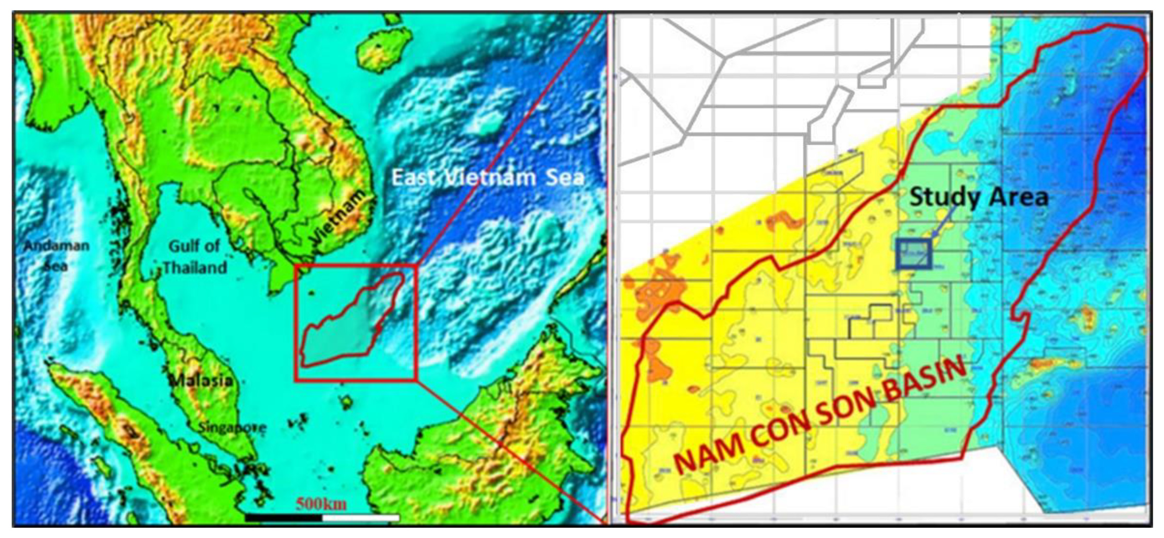
2. Geological Setting
3. Methodology and Dataset
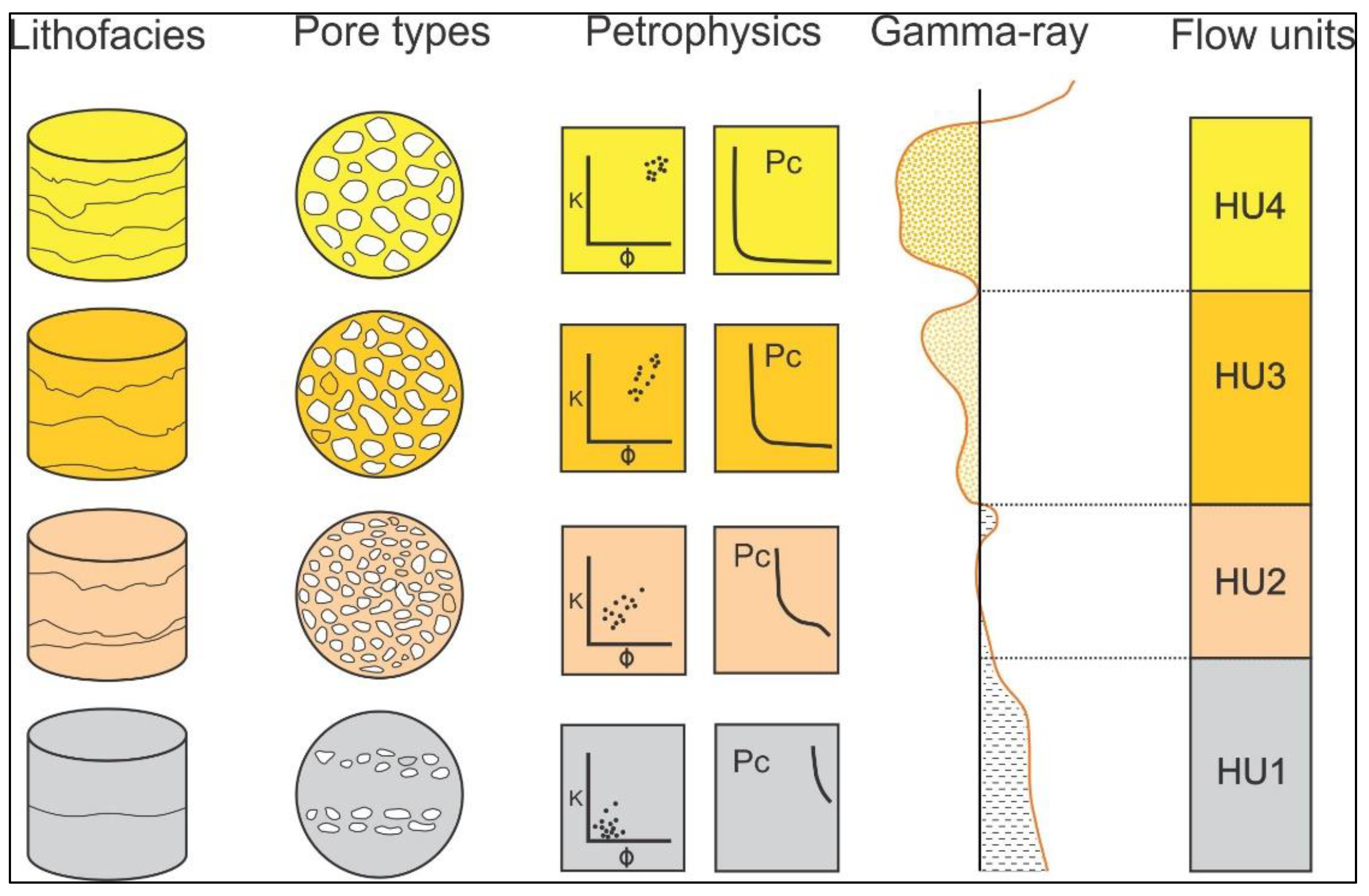
3.1. Hydraulic Flow Unit (HU) Method Overview
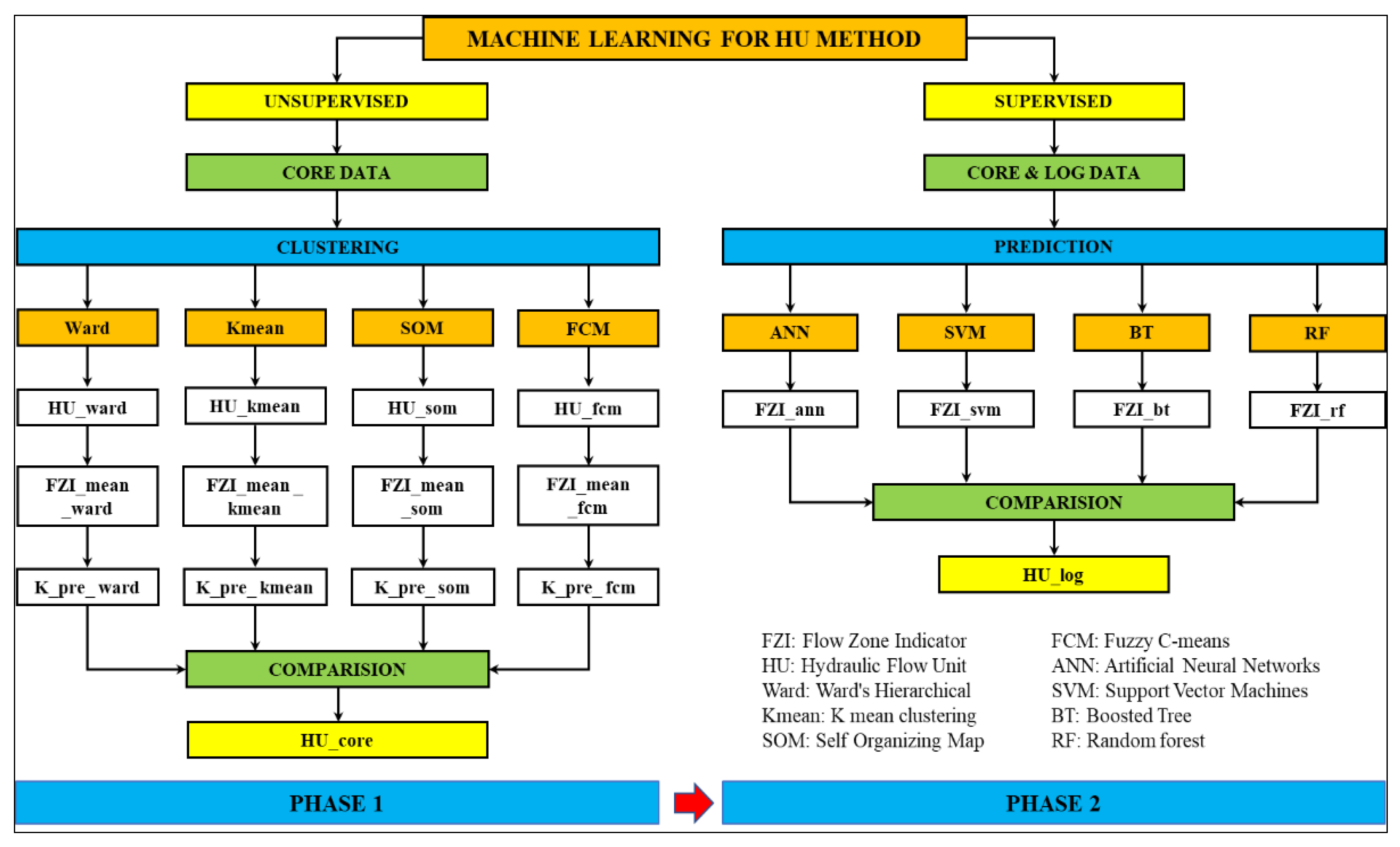
3.2. Applying Machine Learning for Hydraulic Flow Unit Classification and Prediction
3.2.1. Unsupervised Learning Methods
Ward’s Hierarchical Algorithm
- Step 1:
- Calculate the proximity of individual points and consider all the data points as individual clusters,
- Step 2:
- Similar clusters are merged together and form as a single cluster,
- Step 3:
- Recalculate the proximity of new clusters,
- Step 4:
- Repeat steps 2 and 3 until termination conditions are reached.
K-Means Clustering
- Step 1:
- Choose the number of clusters K,
- Step 2:
- Select k random points from the data as center values,
- Step 3:
- Assign all the points to the closest cluster centers,
- Step 4:
- Recompute the new center values,
- Step 5:
- Repeat steps 3 and 4 until termination conditions are reached.
Self-Organizing Map (SOM)
- Step 1:
- Initialize random weight vector,
- Step 2:
- Choose random input vector from the training data,
- Step 3:
- Check all neurons to define the wining one that is the Best Matching Unit (BMU),
- Step 4:
- Update the neuron winner by calculating the neighborhood of the BMU, noting that the amount of neighbors decreases over time,
- Step 5:
- Repeat steps 2–4 until termination conditions are reached.
Fuzzy C-Means Clustering
- Step 1:
- Set number of clusters k,
- Step 2:
- Randomly initialize k center values,
- Step 3:
- Calculate membership degree of each data point,
- Step 4:
- Calculate new center values,
- Step 5:
- Repeat steps 3 and 4 until termination conditions are reached.
3.2.2. Supervised Learning Methods
Support Vector Machines (SVM)
Boosted Trees (BT)
Artificial Neural Network (ANN)
Random Forests (RF)
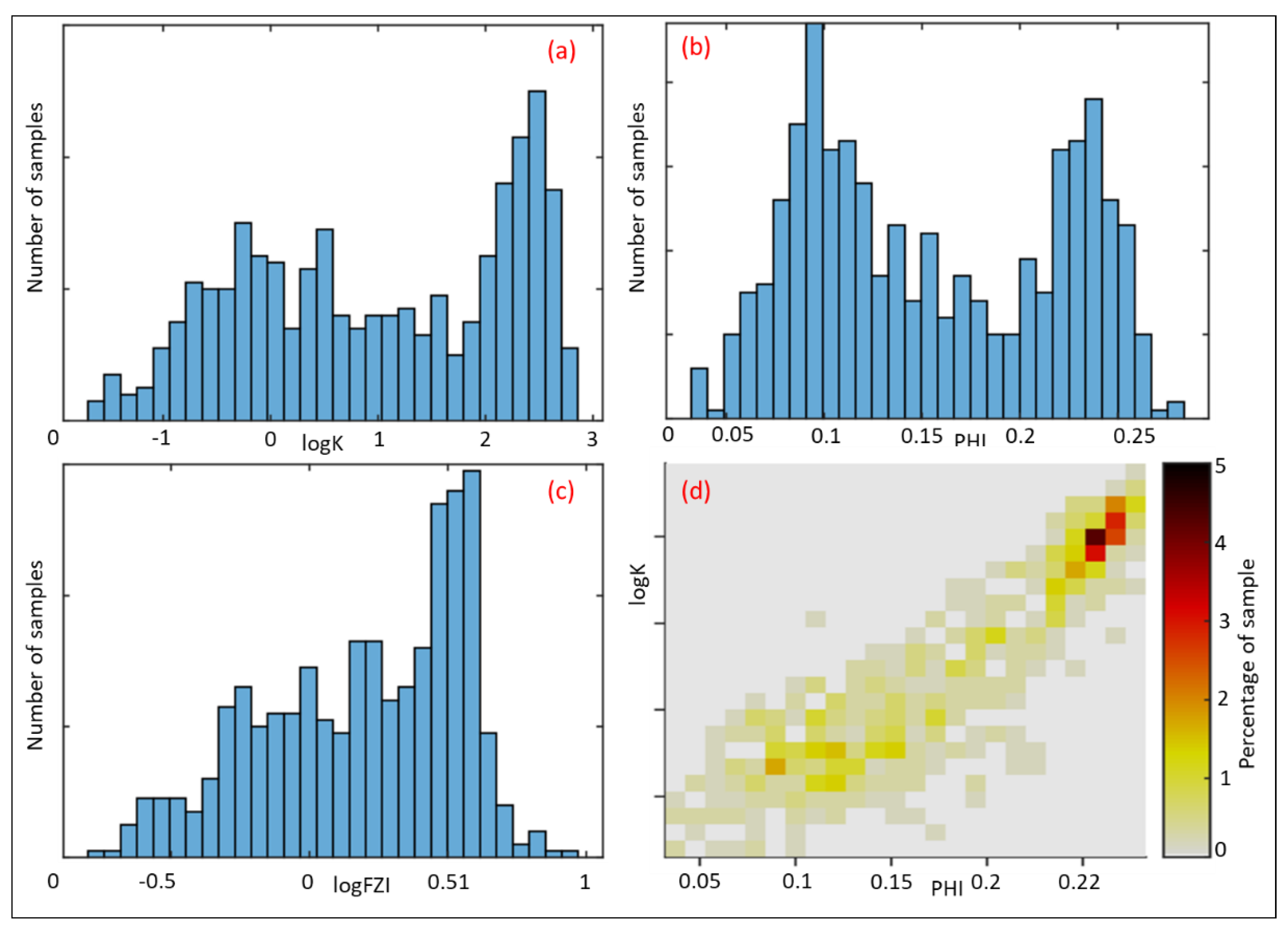
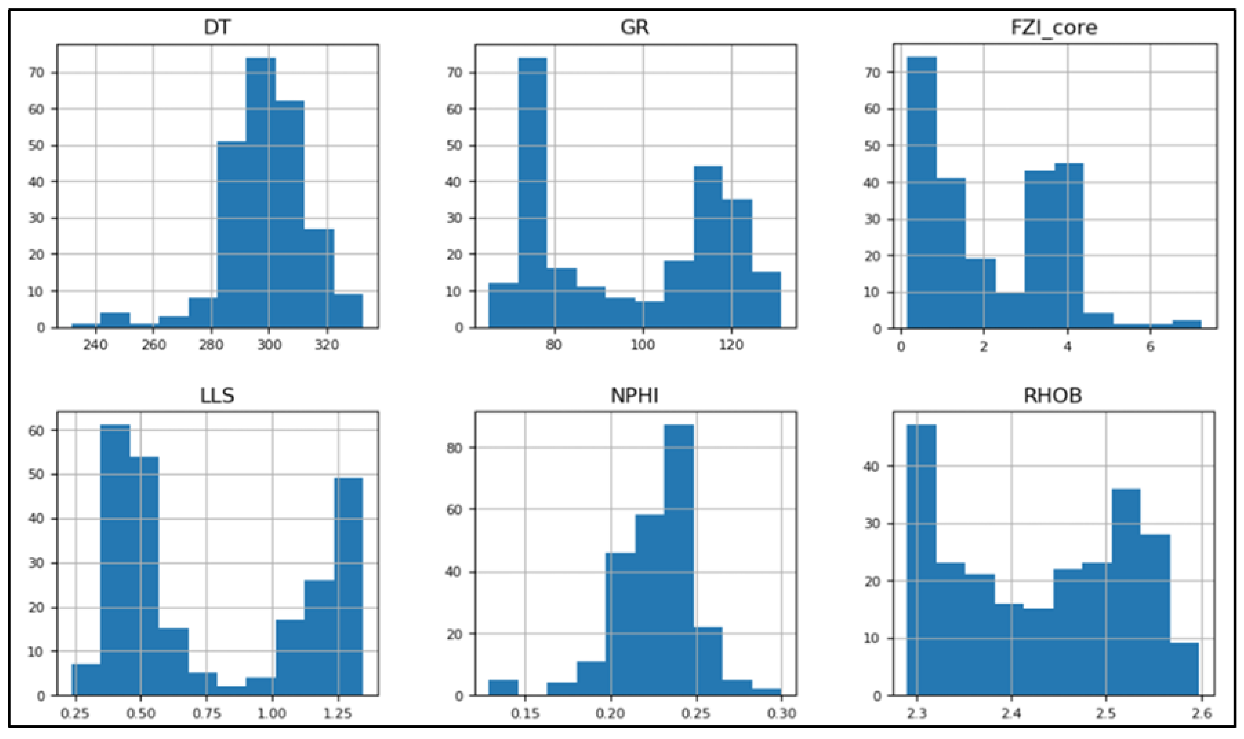
3.3. Dataset
4. Results and Discussion
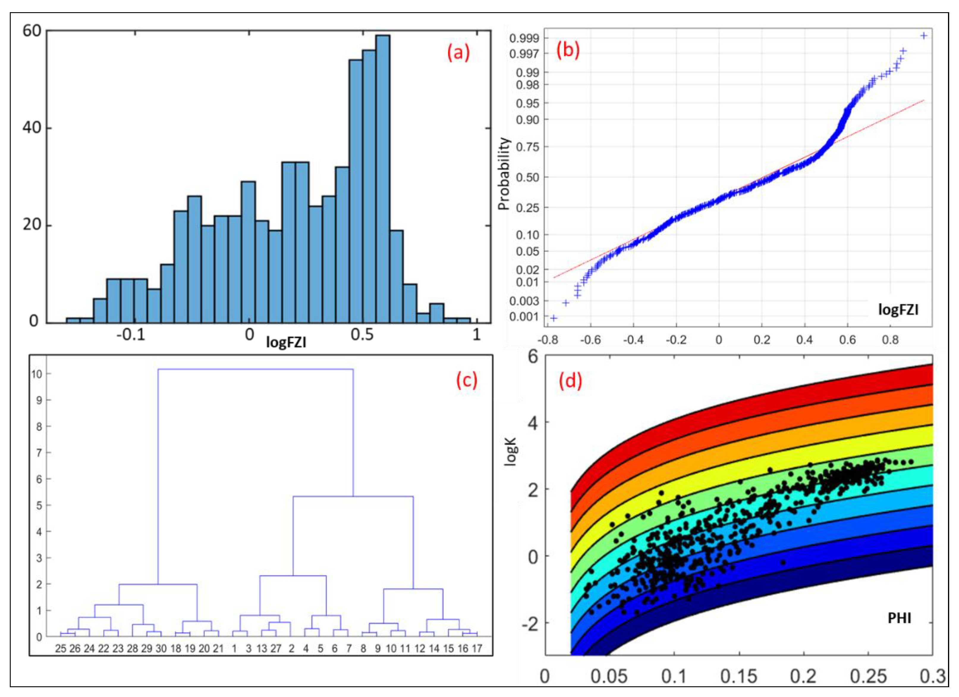
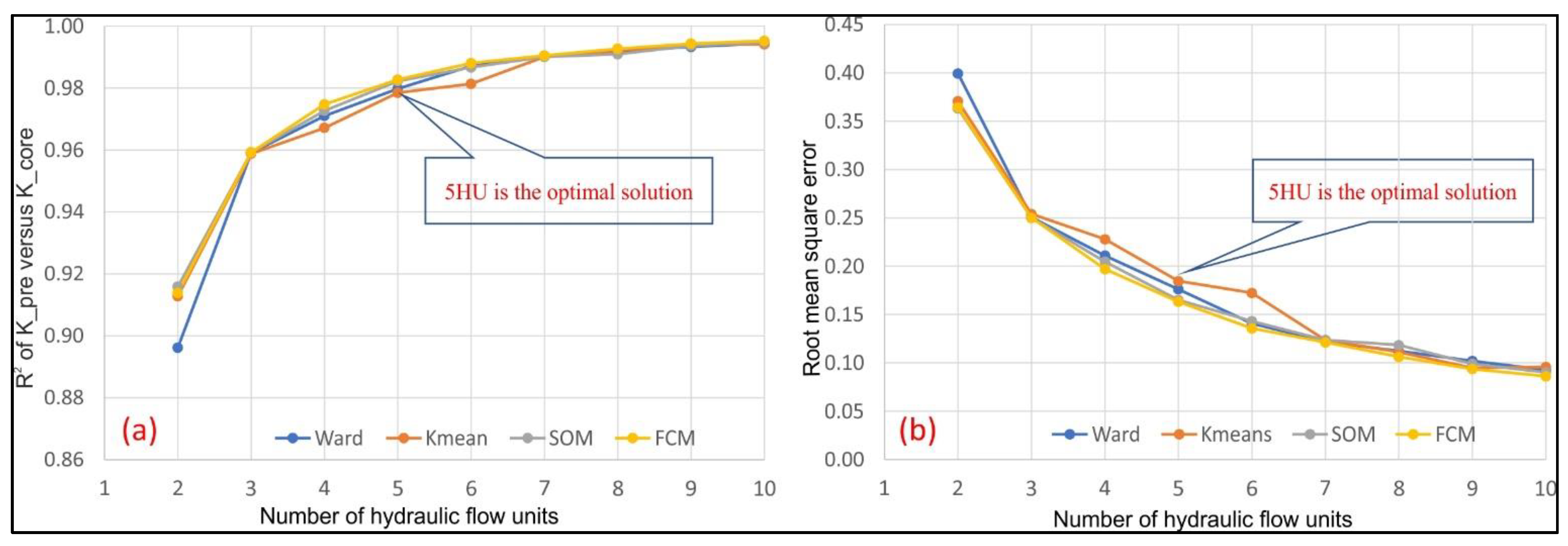
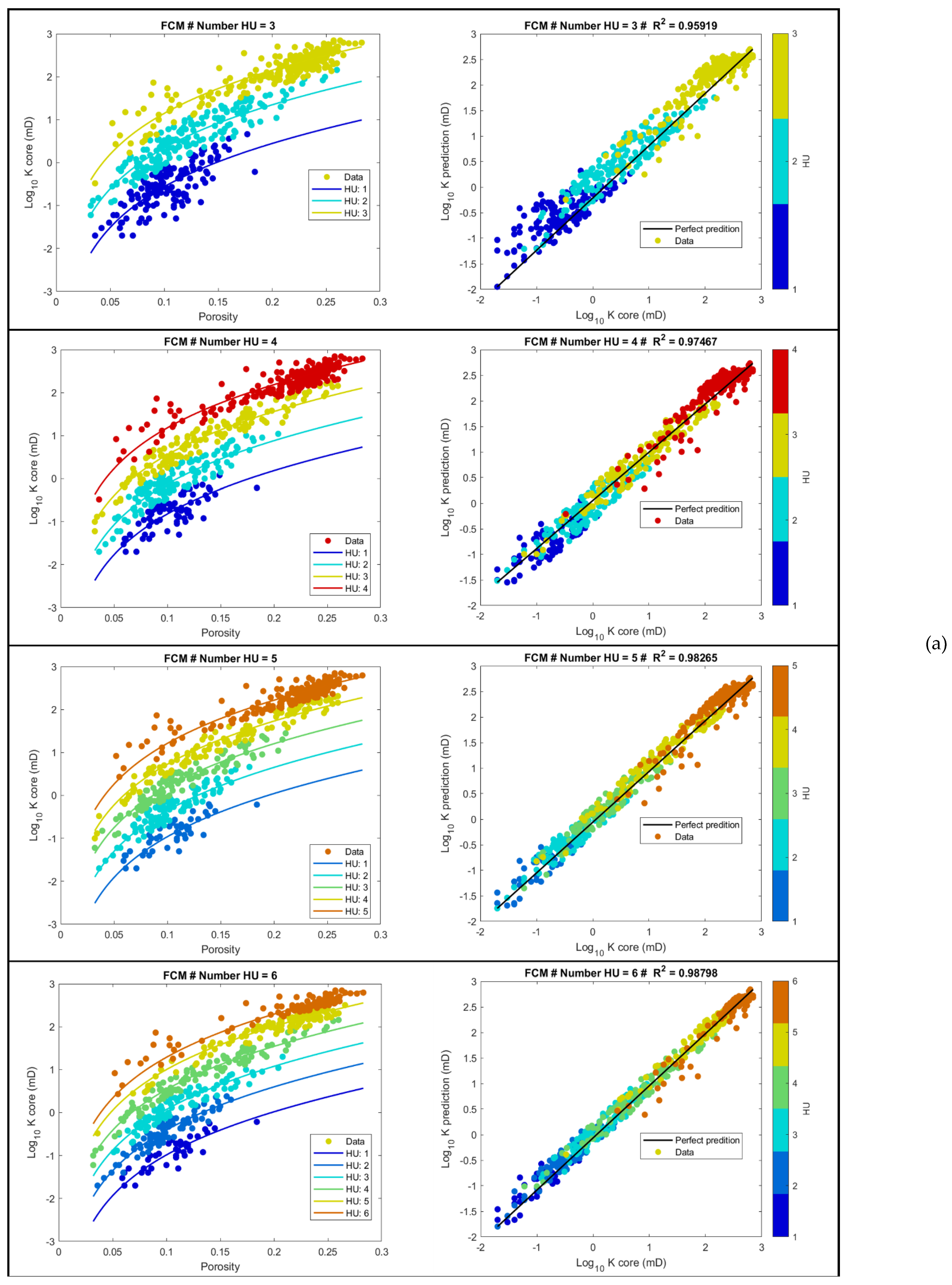
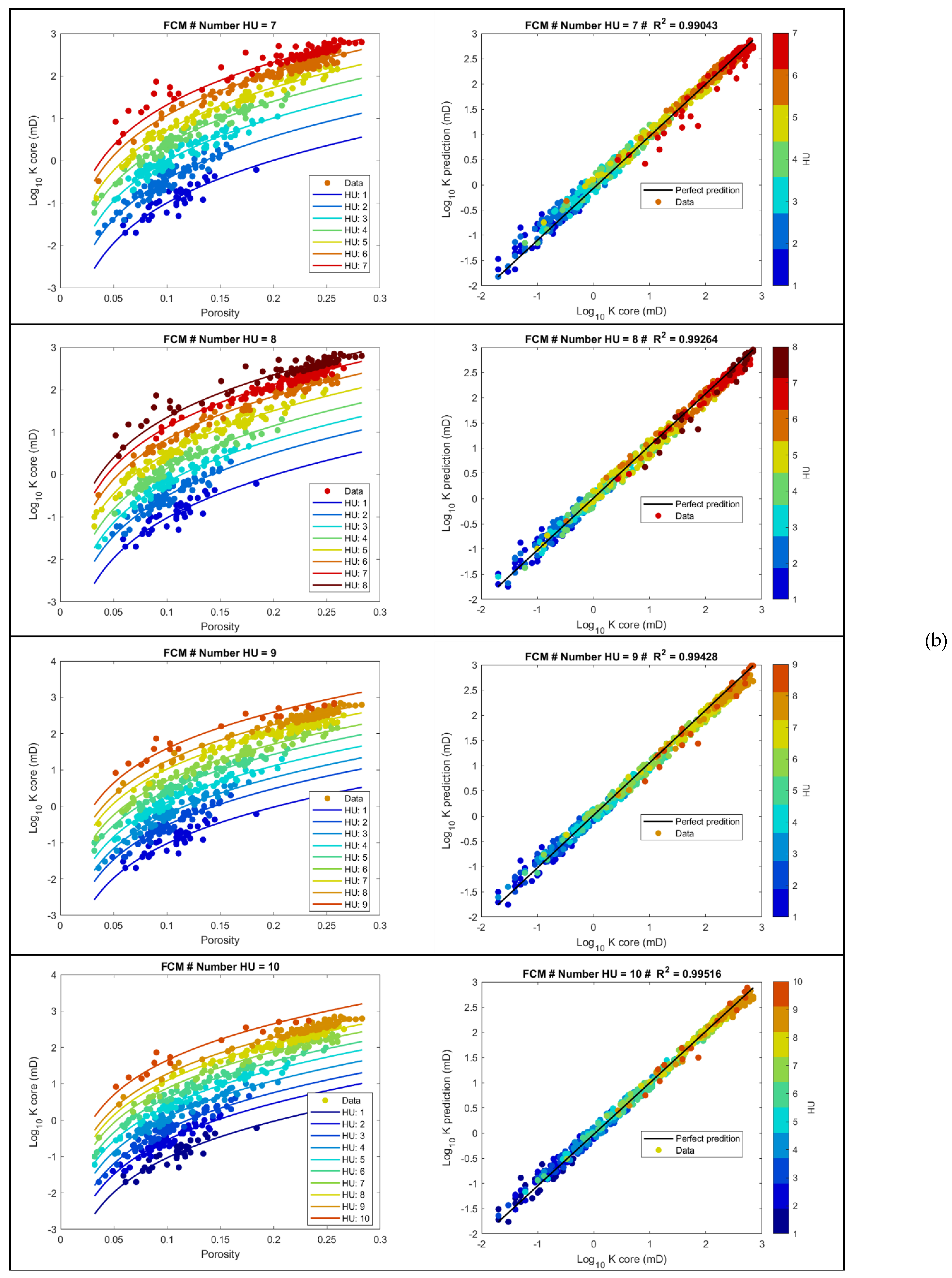
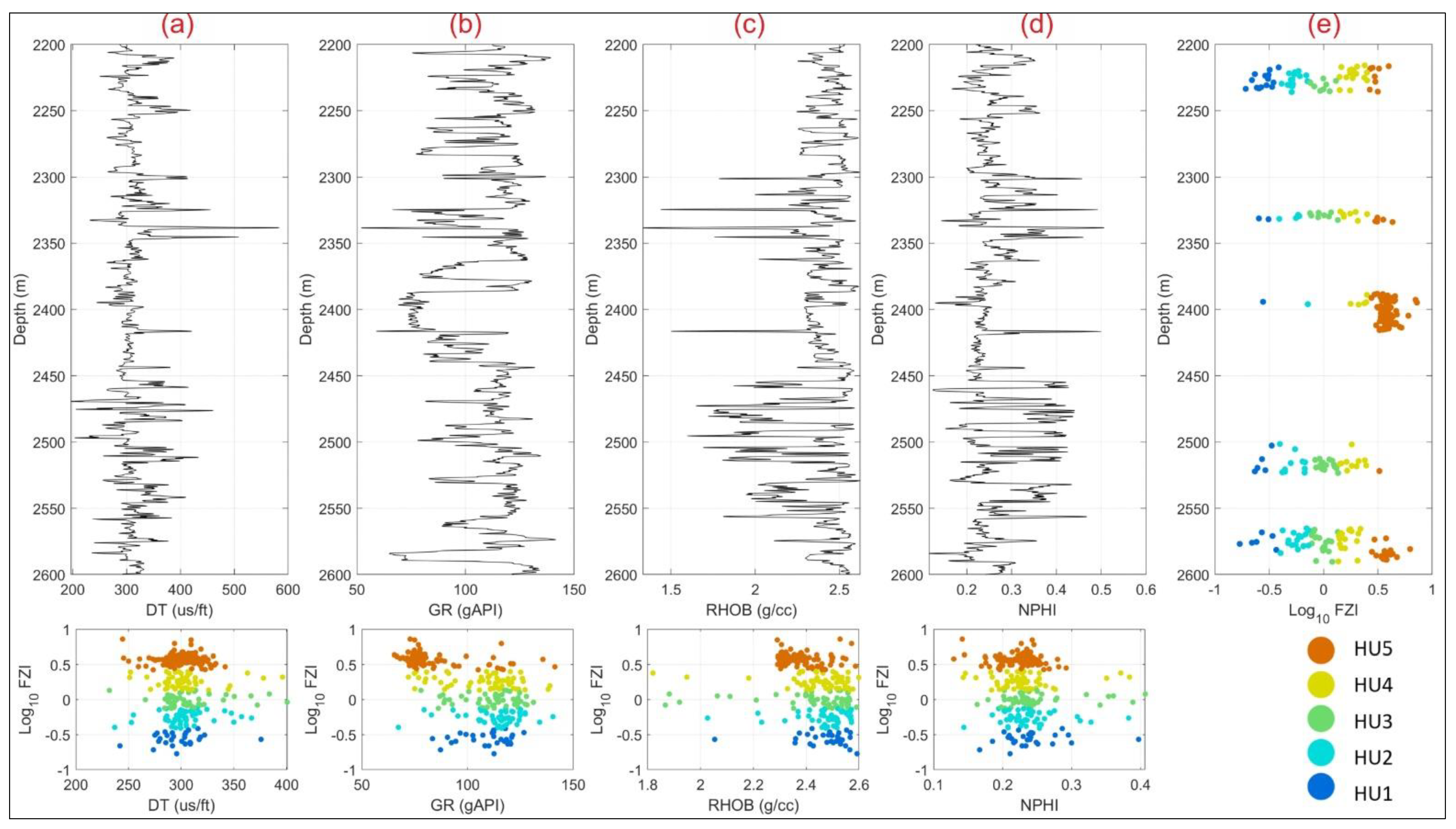
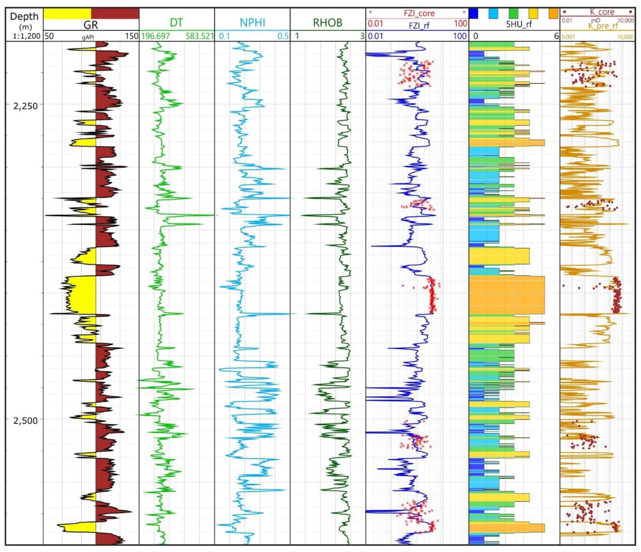
4.1. Unsupervised Machine Learning for HU Core Clustering
4.2. Supervised Machine Learning for HU Logs Prediction
4.2.1. Data Preparation
- -
- Data description,
- -
- Remove outliers,
- -
- Data standardization.
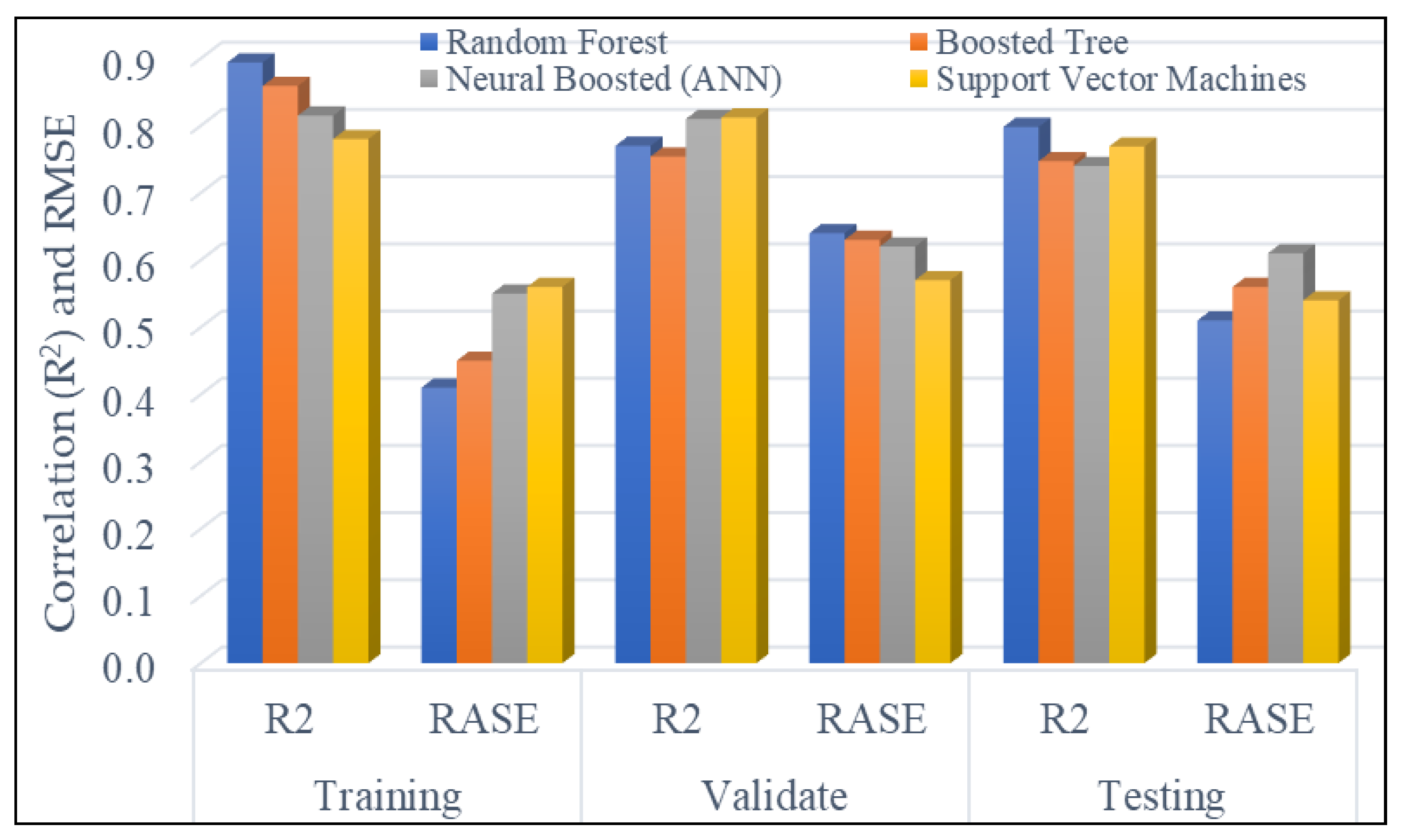
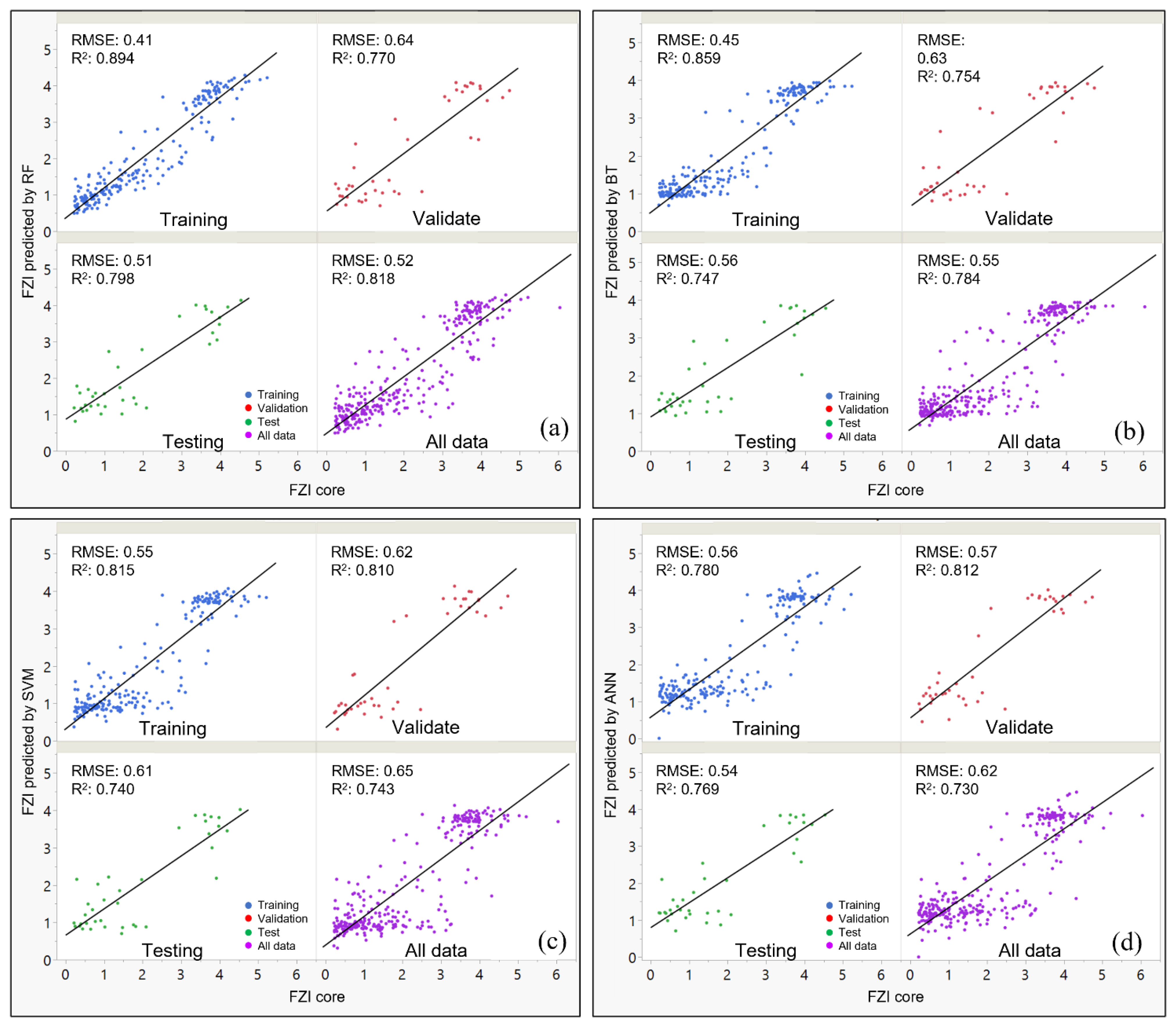
4.2.2. Regression Machine Learning for FZI_log Prediction
- -
- For the R2: For training section, the Random Forest method shows the best result with R2 = 0.894 which is higher than BT (0.859), ANN (0.851) and SVM (0.78). For testing we also see that RF (0.798) is higher than BT (0.747), ANN (0.74) and SVM (0.769) showing better performance (Table 4).
- -
- For the RASE: For training, the Random Forest method shows RASE = 0.41 which is lower than BT (0.45), ANN (0.55) and SVM (0.56), and on testing we also see that RF (0.51) is lower than BT (0.56), ANN (0.61) and SVM (0.54) showing better performance (Table 4).
5. Conclusions
- Unsupervised machine learning is an effective way to quickly organize FZI data into clusters. We used the clustered data to rapidly determine the optimal number of HU groups for reservoir classification.
- We found the best clustering method for HU classification to be the Fuzzy Mean C technique. This showed the optimal division of the Miocene reservoir to be 5 HU.
- We examined four ML techniques. These were RF, ANN, SVM and BT. The RF results were clearly superior.
Author Contributions
Funding
Institutional Review Board Statement
Informed Consent Statement
Data Availability Statement
Acknowledgments
Conflicts of Interest
Abbreviations
| ACE | Alternating Conditional Expectation |
| ANN | Artificial Neural Network |
| BT | Boosted Tree |
| DT | Sonic log |
| FCM | Fuzzy C mean |
| FZI | Flow zone indicator |
| GHE | Global Hydraulic Element |
| GR | Gamma-ray log |
| HU | Hydraulic flow unit |
| K | Permeability |
| LLD | Deep resistivity latero-log |
| LMR | Linear Multiple Regression |
| LSS | Shallow resistivity latero-log |
| NCSB | Nam Con Son Basin |
| NE | North-East |
| NPHI | Neutron porosity |
| PHI | Porosity |
| RF | Random Forest |
| RHOB | Density |
| RQI | Reservoir quality index |
| SOM | Self-Organize Map |
| SVM | Support Vector Machines |
| SW | South-West |
References
- Man, H.Q.; Jarzyna, J. Integration of Core, Well Logging and 2D Seismic Data to Improve a Reservoir Rock Model: A Case Study of Gas Accumulation in the NE Polish Carpathian Foredeep. Geol. Q. 2013, 57, 289–306. [Google Scholar] [CrossRef] [Green Version]
- Abbaszadeh, M.; Fujii, H.; Fujimoto, F. Permeability Prediction by Hydraulic Flow Units—Theory and Applications. SPE Form. Eval. 1996, 11, 263–271. [Google Scholar] [CrossRef]
- Amaefule, J.O.; Altunbay, M.; Tiab, D.; Kersey, D.G.; Keelan, D.K. Enhanced Reservoir Description: Using Core and Log Data to Identify Hydraulic (Flow) Units and Predict Permeability in Uncored Intervals/Wells. In Proceedings of the SPE Annual Technical Conference and Exhibition, Houston, TX, USA, 3–6 October 1993; p. SPE-26436-MS. [Google Scholar]
- Corbett, P.; Ellabad, Y.; Mohammed, K.; Pososyaev, A. Global Hydraulic Elements—Elementary Petrophysics for Reduced Reservoir Modelling. In Proceedings of the 65th EAGE Conference & Exhibition, Stavanger, Norway, 2–5 June 2003; p. cp-6-00256. [Google Scholar]
- Svirsky, D.; Ryazanov, A.; Pankov, M.; Corbett, P.W.M.; Posysoev, A. Hydraulic Flow Units Resolve Reservoir Description Challenges in a Siberian Oil Field. In Proceedings of the SPE Asia Pacific Conference on Integrated Modelling for Asset Management, Kuala Lumpur, Malaysia, 29–30 March 2004; p. SPE-87056-MS. [Google Scholar]
- Guo, G.; Diaz, M.A.; Paz, F.J.; Smalley, J.; Waninger, E.A. Rock Typing as an Effective Tool for Permeability and Water-Saturation Modeling: A Case Study in a Clastic Reservoir in the Oriente Basin. SPE Reserv. Eval. Eng. 2007, 10, 730–739. [Google Scholar] [CrossRef]
- Shenawi, S.; Al-Mohammadi, H.; Faqehy, M. Development of Generalized Porosity-Permeability Transforms by Hydraulic Units for Carbonate Oil Reservoirs in Saudi Arabia. In Proceedings of the SPE/EAGE Reservoir Characterization & Simulation Conference, Abu Dhabi, UAE, 19–21 October 2009. [Google Scholar]
- Shujath Ali, S.; Hossain, M.E.; Hassan, M.R.; Abdulraheem, A. Hydraulic Unit Estimation From Predicted Permeability and Porosity Using Artificial Intelligence Techniques. In Proceedings of the North Africa Technical Conference and Exhibition, Cairo, Egypt, 15–17 April 2013. [Google Scholar]
- Abdallah, S.; Sid Ali, O.; Benmalek, S. Rock type and permeability prediction using flow-zone indicator with an application to Berkine Basin (Algerian Sahara). In SEG Technical Program Expanded Abstracts; Society of Exploration Geophysicists: Dallas, TX, USA, 2016; pp. 3068–3072. [Google Scholar]
- Quang, M.H.; Le An, N.; Jarzyna, J. Hydraulic flow unit classification from core data: Case study of the Z gas reservoir, Poland. JMES 2021, 62, 29–36. [Google Scholar] [CrossRef]
- Ha Quang, M.; Jarzyna, J. Integrating of Core and Logs and 2D Seismic Data to Improve 3D Hydraulic Flow Unit Modeling; European Association of Geoscientists & Engineers: Vienna, Austria, 2011; p. cp-238-00521. [Google Scholar]
- Matyasik, J.; Myśliwiec, M.; Leśniak, G.; Such, P. Relationship between Hydrocarbon Generation and Reservoir Development in the Carpathian Foreland (Poland). In Thrust Belts and Foreland Basins; Springer: Berlin/Heidelberg, Germany, 2007; pp. 413–427. ISBN 978-3-540-69425-0. [Google Scholar]
- Bressan, T.S.; Kehl de Souza, M.; Girelli, T.J.; Junior, F.C. Evaluation of Machine Learning Methods for Lithology Classification Using Geophysical Data. Comput. Geosci. 2020, 139, 104475. [Google Scholar] [CrossRef]
- Al-Mudhafar, W.J. Integrating Well Log Interpretations for Lithofacies Classification and Permeability Modeling through Advanced Machine Learning Algorithms. J. Pet. Explor. Prod. Technol. 2017, 7, 1023–1033. [Google Scholar] [CrossRef] [Green Version]
- Male, F.; Duncan, I.J. Lessons for Machine Learning from the Analysis of Porosity-Permeability Transforms for Carbonate Reservoirs. J. Pet. Sci. Eng. 2020, 187, 106825. [Google Scholar] [CrossRef]
- Al-Mudhafar, W.J. Integrating Component Analysis & Classification Techniques for Comparative Prediction of Continuous & Discrete Lithofacies Distributions. In Proceedings of the Offshore Technology Conference, Houston, TX, USA, 4–7 May 2015; Volume OnePetro; p. OTC-25806-MS. [Google Scholar]
- Al-Mudhafar, W.J. Integrating Kernel Support Vector Machines for Efficient Rock Facies Classification in the Main Pay of Zubair Formation in South Rumaila Oil Field, Iraq. Model. Earth Syst. Environ. 2017, 3, 12. [Google Scholar] [CrossRef]
- Ameur-Zaimeche, O.; Zeddouri, A.; Heddam, S.; Kechiched, R. Lithofacies Prediction in Non-Cored Wells from the Sif Fatima Oil Field (Berkine Basin, Southern Algeria): A Comparative Study of Multilayer Perceptron Neural Network and Cluster Analysis-Based Approaches. J. Afr. Earth Sci. 2020, 166, 103826. [Google Scholar] [CrossRef]
- Tang, H.; White, C.; Zeng, X.; Gani, M.; Bhattacharya, J. Comparison of Multivariate Statistical Algorithms for Wireline Log Facies Classification. In Proceedings of the AAPG Annual Meeting, Dallas, TX, USA, 30 June–1 July 2004. [Google Scholar]
- Baldwin, J.L.; Bateman, R.M.; Wheatley, C.L. Application Of A Neural Network To The Problem Of Mineral Identification From Well Logs. Log Anal. 1990, 31, SPWLA-1990-v31n5a1. [Google Scholar]
- Rogers, S.J.; Fang, J.H.; Karr, C.L.; Stanley, D.A. Determination of Lithology from Well Logs Using a Neural Network1. AAPG Bull. 1992, 76, 731–739. [Google Scholar] [CrossRef]
- Wong, P.M.; Jian, F.X.; Taggart, I.J. A Critical Comparison of Neural Networks and Discriminant Analysis in Lithofacies, Porosity and Permeability Predictions. J. Pet. Geol. 1995, 18, 191–206. [Google Scholar] [CrossRef]
- Avseth, P.; Mukerji, T. Seismic Lithofacies Classification From Well Logs Using Statistical Rock Physics. Petrophys.-SPWLA J. Form. Eval. Reserv. Descr. 2002, 43, SPWLA-2002-v43n2a1. [Google Scholar]
- Dubois, M.K.; Bohling, G.C.; Chakrabarti, S. Comparison of Four Approaches to a Rock Facies Classification Problem. Comput. Geosci. 2007, 33, 599–617. [Google Scholar] [CrossRef]
- Wood, D.A. Lithofacies and Stratigraphy Prediction Methodology Exploiting an Optimized Nearest-Neighbour Algorithm to Mine Well-Log Data. Mar. Pet. Geol. 2019, 110, 347–367. [Google Scholar] [CrossRef]
- Dung, B.V.; Tuan, H.A.; Van Kieu, N.; Man, H.Q.; Thanh Thuy, N.T.; Dieu Huyen, P.T. Depositional Environment and Reservoir Quality of Miocene Sediments in the Central Part of the Nam Con Son Basin, Southern Vietnam Shelf. Mar. Pet. Geol. 2018, 97, 672–689. [Google Scholar] [CrossRef]
- Tuan, N.Q.; Tri, T.V. Seismic Interpretation of the Nam Con Son Basin and Its Implication for the Tectonic Evolution. Indones. J. Geosci. 2016, 3, 127–137. [Google Scholar] [CrossRef] [Green Version]
- An, N.H. Assessement of Improved Oil Recovery Potential of Dai Hung Oil Field. Petrovietnam J. 2008, 8, 53–61. [Google Scholar] [CrossRef]
- Ebanks, W.J., Jr. Flow Unit Concept—Integrated Approach to Reservoir Description for Engineering Projects: Abstract. AAPG Bull. 1987, 71, 551–552. [Google Scholar]
- Ebanks, W.J., Jr.; Scheiling, M.H.; Atkinson, C.D. Flow Units for Reservoir Characterization; Morton-Thompson, D., Ed.; Development Geology Reference Manual; AAPG: Tulsa, OK, USA, 1992; ISBN 978-0-89181-660-7. [Google Scholar]
- Kozeny, J. Uber Kapillare Letung Des Wassers Im Boden, Sitzungsberichte. R. Acad. Sci. 1927, 136, 271–306. [Google Scholar]
- Carman, P.C. Fluid Flow through Granular Beds. Trans. Inst. Chem. Eng. 1937, 15, 150–167. [Google Scholar] [CrossRef]
- Jarzyna, J.; Man, H.Q. Hydraulic Units Differentiated in Reservoir Rock to Facilitate Permeability Determinations for Flow Modeling in Gas Deposit. Prz. Geol. 2009, 57, 996–1003. [Google Scholar]
- Saxena, A.; Prasad, M.; Gupta, A.; Bharill, N.; Patel, O.P.; Tiwari, A.; Er, M.J.; Ding, W.; Lin, C.-T. A Review of Clustering Techniques and Developments. Neurocomputing 2017, 267, 664–681. [Google Scholar] [CrossRef] [Green Version]
- Abbas, M.A.; Al Lawe, E.M. Clustering Analysis and Flow Zone Indicator for Electrofacies Characterization in the Upper Shale Member in Luhais Oil Field, Southern Iraq. In Proceedings of the Abu Dhabi International Petroleum Exhibition & Conference, Abu Dhabi, UAE, 12 November 2019. [Google Scholar]
- Kohonen, T. The Self-Organizing Map. Proc. IEEE 1990, 78, 1464–1480. [Google Scholar] [CrossRef]
- Dixit, N.; McColgan, P.; Kusler, K. Machine Learning-Based Probabilistic Lithofacies Prediction from Conventional Well Logs: A Case from the Umiat Oil Field of Alaska. Energies 2020, 13, 4862. [Google Scholar] [CrossRef]
- Suganya, R.; Shanthi, R. Fuzzy C-Means Algorithm—A Review. Int. J. Sci. Res. Publ. 2012, 2, 3. [Google Scholar]
- Vapnik, V. Pattern Recognition Using Generalized Portrait Method. Autom. Remote Control 1963, 24, 774–780. [Google Scholar]
- Vapnik, V. A Note on One Class of Perceptrons. Autom. Remote Control 1964, 24, 821–837. [Google Scholar]
- Rodriguez-Galiano, V.; Sanchez-Castillo, M.; Chica-Olmo, M.; Chica-Rivas, M. Machine Learning Predictive Models for Mineral Prospectivity: An Evaluation of Neural Networks, Random Forest, Regression Trees and Support Vector Machines. Ore Geol. Rev. 2015, 71, 804–818. [Google Scholar] [CrossRef]
- Kaftannikov, I.L.; Parasich, A.V. Decision Tree’s Features of Application in Classification Problems. Bull. S. Ural State Univ. Ser. Comput. Technol. Autom. Control Radioelectron. 2015, 15, 26–32. [Google Scholar] [CrossRef] [Green Version]
- Salakhutdinova, K.I.; Lebedev, I.S.; Krivtsova, I.E. Gradient Boosting Trees Method in the Task of Software Identification. Sci. Tech. J. Inf. Technol. Mech. Opt. 2018, 18, 1016–1022. [Google Scholar] [CrossRef]
- Freund, Y.; Schapire, R.E. Experiments with a New Boosting Algorithm; Morgan Kaufmann Publishers Inc.: Bari, Italy, 1996; pp. 148–156. [Google Scholar]
- Jothilakshmi, S.; Gudivada, V.N. Chapter 10—Large Scale Data Enabled Evolution of Spoken Language Research and Applications. In Handbook of Statistics; Gudivada, V.N., Raghavan, V.V., Govindaraju, V., Rao, C.R., Eds.; Elsevier: Amsterdam, The Netherlands, 2016; Volume 35, pp. 301–340. ISBN 0169-7161. [Google Scholar]
- Pavlov, J.L. Limit Theorems for the Number of Trees of a given Size in a Random Forest. Math. USSR-Sb. 1977, 32, 335–345. [Google Scholar] [CrossRef]
- Pavlov, Y.L. The Asymptotic Distribution of Maximum Tree Size in a Random Forest. Theory Probab. Its Appl. 1978, 22, 509–520. [Google Scholar] [CrossRef]
- Pavlov, Y.L. Random Forests; VSP: Utrecht, The Netherlands, 2000; ISBN 90-6764-314-9. [Google Scholar]
- Breiman, L. Random Forests. Mach. Learn. 2001, 45, 5–32. [Google Scholar] [CrossRef] [Green Version]
- Chistiakov, S.P. Random Forests: An Overview. Proc. Karelian Sci. Cent. Russ. Acad. Sci. 2013, 4, 117–136. [Google Scholar]
- Corbett, P.; Potter, D. Petrotyping: A Basemap and Atlas for Navigating through Permeability and Porosity Data for Reservoir Comparison and Permeability Prediction. In Proceedings of the International Symposium of the Society of Core Analysts (SCA2004-30), Abu Dhabi, UAE, 5–9 October 2004. [Google Scholar]
- Breunig, M.M.; Kriegel, H.P.; Ng, R.T.; Sander, J. LOF: Identifying DensityBased Local Outliers. SIGMOD Rec. 2000, 29, 93–104. [Google Scholar] [CrossRef]


| HU | Correlation Coefficient (R2) | Root Mean Square Error (RMSE) | ||||||
|---|---|---|---|---|---|---|---|---|
| Ward | Kmean | SOM | FCM | Ward | Kmean | SOM | FCM | |
| 2 | 0.896 | 0.913 | 0.916 | 0.914 | 0.399 | 0.371 | 0.363 | 0.364 |
| 3 | 0.959 | 0.959 | 0.959 | 0.959 | 0.251 | 0.254 | 0.250 | 0.250 |
| 4 | 0.971 | 0.967 | 0.973 | 0.975 | 0.211 | 0.228 | 0.205 | 0.197 |
| 5 | 0.980 | 0.978 | 0.982 | 0.983 | 0.176 | 0.184 | 0.165 | 0.163 |
| 6 | 0.987 | 0.981 | 0.987 | 0.988 | 0.141 | 0.172 | 0.143 | 0.136 |
| 7 | 0.990 | 0.990 | 0.990 | 0.990 | 0.122 | 0.124 | 0.124 | 0.121 |
| 8 | 0.992 | 0.992 | 0.991 | 0.993 | 0.112 | 0.111 | 0.118 | 0.106 |
| 9 | 0.993 | 0.994 | 0.994 | 0.994 | 0.102 | 0.095 | 0.099 | 0.094 |
| 10 | 0.994 | 0.994 | 0.995 | 0.995 | 0.093 | 0.096 | 0.090 | 0.086 |
| 5 HU | Cores Number | PHI (%) | K(mD) | FZI | ||||||
|---|---|---|---|---|---|---|---|---|---|---|
| Min | Mean | Max | Min | Mean | Max | Min | Mean | Max | ||
| HU1 | 46 | 0.059 | 0.106 | 0.184 | 0.020 | 0.178 | 0.620 | 0.169 | 0.311 | 0.417 |
| HU2 | 101 | 0.036 | 0.103 | 0.177 | 0.020 | 0.737 | 4.600 | 0.420 | 0.614 | 0.817 |
| HU3 | 111 | 0.032 | 0.114 | 0.211 | 0.060 | 4.109 | 28.000 | 0.821 | 1.149 | 1.518 |
| HU4 | 124 | 0.032 | 0.158 | 0.260 | 0.100 | 47.248 | 206.000 | 1.522 | 2.068 | 2.699 |
| HU5 | 205 | 0.052 | 0.213 | 0.283 | 2.700 | 250.558 | 699.000 | 2.748 | 3.675 | 9.042 |
| Statistic | DT | GR | LLD | LLS | NPHI | RHOB | FZI_Core |
|---|---|---|---|---|---|---|---|
| mean | 300.333 | 97.972 | 13.429 | 7.953 | 0.228 | 2430.912 | 2.172 |
| std. | 14.479 | 19.528 | 13.521 | 6.804 | 0.023 | 90.2910 | 1.503 |
| min | 245.294 | 66.490 | 2.123 | 1.719 | 0.146 | 2290.071 | 0.169 |
| 25% | 292.010 | 77.450 | 3.441 | 2.799 | 0.214 | 2338.267 | 0.750 |
| 50% | 300.792 | 99.962 | 5.264 | 3.525 | 0.231 | 2434.221 | 1.811 |
| 75% | 308.826 | 115.844 | 23.858 | 14.546 | 0.241 | 2512.406 | 3.615 |
| max | 341.662 | 141.292 | 42.937 | 22.291 | 0.300 | 2591.491 | 7.030 |
| Supervised Methods | Training | Validate | Testing | |||
|---|---|---|---|---|---|---|
| R2 | Rase | R2 | Rase | R2 | Rase | |
| Random Forest | 0.894 | 0.410 | 0.770 | 0.640 | 0.798 | 0.510 |
| Boosted Tree | 0.859 | 0.450 | 0.754 | 0.630 | 0.747 | 0.560 |
| Neural Boosted (ANN) | 0.815 | 0.550 | 0.810 | 0.620 | 0.740 | 0.610 |
| Support Vector Machines | 0.780 | 0.560 | 0.812 | 0.570 | 0.769 | 0.540 |
Publisher’s Note: MDPI stays neutral with regard to jurisdictional claims in published maps and institutional affiliations. |
© 2021 by the authors. Licensee MDPI, Basel, Switzerland. This article is an open access article distributed under the terms and conditions of the Creative Commons Attribution (CC BY) license (https://creativecommons.org/licenses/by/4.0/).
Share and Cite
Man, H.Q.; Hien, D.H.; Thong, K.D.; Dung, B.V.; Hoa, N.M.; Hoa, T.K.; Kieu, N.V.; Ngoc, P.Q. Hydraulic Flow Unit Classification and Prediction Using Machine Learning Techniques: A Case Study from the Nam Con Son Basin, Offshore Vietnam. Energies 2021, 14, 7714. https://doi.org/10.3390/en14227714
Man HQ, Hien DH, Thong KD, Dung BV, Hoa NM, Hoa TK, Kieu NV, Ngoc PQ. Hydraulic Flow Unit Classification and Prediction Using Machine Learning Techniques: A Case Study from the Nam Con Son Basin, Offshore Vietnam. Energies. 2021; 14(22):7714. https://doi.org/10.3390/en14227714
Chicago/Turabian StyleMan, Ha Quang, Doan Huy Hien, Kieu Duy Thong, Bui Viet Dung, Nguyen Minh Hoa, Truong Khac Hoa, Nguyen Van Kieu, and Pham Quy Ngoc. 2021. "Hydraulic Flow Unit Classification and Prediction Using Machine Learning Techniques: A Case Study from the Nam Con Son Basin, Offshore Vietnam" Energies 14, no. 22: 7714. https://doi.org/10.3390/en14227714