Article

A Novel Short-Term Residential Electric Load Forecasting Method Based on Adaptive Load Aggregation and Deep Learning Algorithms

1
Economics and Technology Research Institute, State Grid Hubei Electric Power Company, Wuhan 430077, China
2
School of Automation, Wuhan University of Technology, Wuhan 430070, China
*
Author to whom correspondence should be addressed.
Energies 2021, 14(22), 7820; https://doi.org/10.3390/en14227820
Submission received: 28 September 2021 / Revised: 28 October 2021 / Accepted: 9 November 2021 / Published: 22 November 2021
(This article belongs to the Special Issue Artificial Intelligence for Buildings)

Abstract

:
Short-term residential load forecasting is the precondition of the day-ahead and intra-day scheduling strategy of the household microgrid. Existing short-term electric load forecasting methods are mainly used to obtain regional power load for system-level power dispatch. Due to the high volatility, strong randomness, and weak regularity of the residential load of a single household, the mean absolute percentage error (MAPE) of the traditional methods forecasting results would be too big to be used for home energy management. With the increase in the total number of households, the aggregated load becomes more and more stable, and the cyclical pattern of the aggregated load becomes more and more distinct. In the meantime, the maximum daily load does not increase linearly with the increase in households in a small area. Therefore, in our proposed short-term residential load forecasting method, an optimal number of households would be selected adaptively, and the total aggregated residential load of the selected households is used for load prediction. In addition, ordering points to identify the clustering structure (OPTICS) algorithm are also selected to cluster households with similar power consumption patterns adaptively. It can be used to enhance the periodic regularity of the aggregated load in alternative. The aggregated residential load and encoded external factors are then used to predict the load in the next half an hour. The long short-term memory (LSTM) deep learning algorithm is used in the prediction because of its inherited ability to maintain historical data regularity in the forecasting process. The experimental data have verified the effectiveness and accuracy of our proposed method.

1. Introduction

The different kinds of appliances have increased significantly in households, and the residential electrical load has maintained a medium–high growth rate over the years. In the meantime, with the development of renewable energy technologies, rooftop photovoltaic and distributed electric vehicles are also widely involved in home energy management [1,2,3]. Therefore, the household microgrid will be established by household appliances, rooftop photovoltaic, distributed electric vehicles, and battery energy storage devices [4,5,6]. The constructed household microgrid can dispatch the residential electricity flexibly, provide demand-side response capability, and, finally, improve the economic performance of the microgrid operational management.
Short-term residential load forecasting is the precondition of the day-ahead and intra-day scheduling strategy of the household microgrid. Accurate short-term load forecasting results can be used to form a more reasonable home energy scheduling plan [7,8,9]. Since dispatching management is only applied in the large-scale regions in the traditional power grid, existing electric load forecasting methods are mainly used to obtain regional power load for generation scheduling, transaction scheduling, and network dispatching [10,11]. These load forecasting methods can be mainly grouped into three categories, including similar day or similar time interval-based forecasting methods, frequency component-based forecasting methods, and meteorological factor-based load forecasting methods.
Similar day or similar time interval-based load forecasting methods use the historical load data at the same time in the related and nearby days to obtain the load value at some time on the prediction day [12]. In these methods, similar day identification and data smoothing algorithms are the most important procedures. Algorithms such as Euclid distance or density clustering have been proposed and used to find the most suitable similar day or similar time interval [12,13]. In the meantime, several data smoothing algorithms are also applied in the forecasting process to efficiently find the laws of the relevant historical data and the forecasting load value on the prediction day, including the least square regression algorithm [14], support vector machine [15], artificial neural network [16], etc. The principle of these methods is essentially based on the electrical consumption patterns on the day of the week, which are directly determined by human activity. Nowadays, these methods are easy to realize and widely applied in the field.
Frequency component-based forecasting methods would decompose the electric load series into components with daily periodicity, weekly periodicity, climate-vulnerable low frequency, and randomness-determined high frequency. In addition, corresponding algorithms are optimally designed to forecast these several components separately. In references [17,18,19,20], variational mode decomposition and wavelet transform algorithms are used to decompose time series load data separately into several components with different frequencies. These methods use the power consumption patterns of all components instead of the entire load regularity. The influence of the random and abnormal load disturbance on the forecasting result can be reduced because of the effective decomposition and special signal processing for different components.
In contrast to the first and second kinds of methods, meteorological parameters are directly used as input factors in meteorological factor-based load forecasting methods. In these methods, in addition to historical time series of electric load, intraday meteorological parameters and accumulative effect factors of historical meteorological parameters are specially converted to several input variables by numerical value mapping [21,22,23,24]. These variables are combined with the power consumption data to form multi-dimensional input parameters for the following forecasting algorithms, including artificial neural network [21,22,23], support vector machine [24], and the mutation of these two algorithms. This kind of method intensifies the influence of the meteorological parameters on the electric load forecasting, and then the prediction accuracy can be further improved and the forecasting error can be reduced.
The abovementioned three kinds of short-term electric load forecasting methods have been widely applied in the field for system-level load forecasting over the years. The forecasting error of the power consumption in the whole country, province, or city can be controlled under 0.5%, as stated in some reports [25]. The precondition of all these methods is that the predicted load should have a remarkably regular pattern. Due to the randomness of human activities, the residential electric load of a single-family dwelling or limited multi-family houses has high fluctuation and ruleless trajectory. Therefore, when traditional electric load forecasting methods are applied in home energy management, the mean absolute percentage error (MAPE) would be greater than 40% [26].
Different from the summing electric load in a city or a region, volatility and uncertainty exist in residential power consumption. The external factors, including the routine of life, human occupancy, and household appliances, will directly affect the short-term individual power consumption. Reference [27] analyzes the characteristics of residential electric load based on the nature of different appliances and the routine of life. Due to the burdensome and insatiable data collection, a physical model is automatically inferior to the data-driven electric load forecasting model. With the development of the smart meter and Internet of Things technologies [28], data-driven residential load forecasting algorithms have gained the attention of scholars. References [29,30] summarize the data-driven forecasting methods that are applied in building energy management. In these methods, feature generation from the daily timetable, clustering algorithms, and deep learning networks are used to forecast the building energy consumption. In [31], convolutional neural networks (CNN) and long short-term memory neural networks (LSTM) are combined to forecast the electric load of a four-story building robustly and reliably. To improve the LSTM capability to deal with the varying length of input features, the attention mechanism is integrated into the LSTM algorithm to improve the prediction performance [32]. The attention mechanism is also used to improve the prediction accuracy for a sudden increase in power usage [33]. Compared with the load prediction of a whole building or a whole floor, the electric load prediction at a single-unit level is more difficult because of the greater randomness. In [34], an LSTM algorithm is used to achieve power consumption patterns and human behaviors in real time. It can improve the load prediction adaptivity in home appliances configuration. Furthermore, appliance consumption sequences are integrated into the LSTM algorithm to especially improve prediction accuracy for the volatile problem in [35]. In the meantime, modified LSTM algorithms are also proposed in [36,37] to adaptively assign weights to temporal features and extract spatial characteristics effectively. These methods provide several effective algorithms to forecast the individual electric load, and the prediction process can be adopted for reference by future research. However, the prediction results show that the prediction error for a single unit is still too big to be applied in the field. The mean absolute percentage error (MAPE) nearly reaches 30–40% for different experimental data. Therefore, the prediction load results cannot be directly used for home energy management.
In this paper, a novel short-term residential load forecasting framework will be proposed to fill the gap between the electric load forecasting of a single-family unit and that of a whole city. Firstly, characteristic analysis of residential electric loads will be conducted to verify the necessity of load aggregating. Secondly, an optimal aggregated electric load algorithm is proposed and discussed by using typical load clustering algorithms. Thirdly, a LSTM-based residential load forecasting model is proposed and discussed with the input parameters of the adaptive load aggregation and the encoded external factors. The experimental data has verified the effectiveness and accuracy of our proposed method.

2. Power Consumption Analysis of Household Appliances

The residential electric load consists of different home appliances. These residential electric loads can be grouped into three categories. The first kind of load works at a relatively consistent time every day, including appliances such as rice cookers, kitchen ventilators, and refrigerators. The second kind of load is directly determined by external factors, including heating, air-conditioning, and electric fans. The third kind of load would work every day, but the corresponding operation time would vary and be influenced by the routine life of the host family, including the electric water heater and laundry machine.
Nowadays, the residential electric load is mainly collected by intelligent electric meters and used by the marketing departments of electric utilities. Globally, the sampling intervals of residential load are in the range of 15 min to one hour in the field [38]. In this section, the historical data of residential electric load would be analyzed to obtain the statistical characteristics based on typical quantitative indicators.

2.1. Quantitative Indicators of Residential Electric Loads

Based on the collected historical data and the requirement of load prediction, the following five indicators would be used to describe the characteristics of residential electric load.
(1) maximum daily load
The maximum daily load is the maximum value of selected residential electric load in a whole day and is represented by Pmax in this paper.
(2) mean daily load
The mean daily load is the mean value of selected residential electric load in a whole day and is represented by Pv in this paper. It will be calculated by
P υ = 1 N × Δ t i = 1 N P i × Δ t
where Pi represents the ith sampling data of selected residential electric load, Δ t represents the sampling interval of the smart meter, N represents the total sampling number in a whole day, and N × Δ t equals 24 h.
(3) mean daily loading rate
The mean daily loading rate, γ, is the ratio of mean daily load to the maximum daily load, which is expressed by
γ = P υ P m a x
(4) minimum daily loading rate
The minimum daily loading rate, β, is the ratio of minimum daily load, Pmin, to the maximum daily load, Pmax, and is calculated by
β = P m i n P m a x
(5) daily volatility index
The dispersion degree of sample data is usually analyzed and obtained by statistical analysis technique. The coefficient of dispersion can be used to analyze the volatility of the daily electric load. The daily volatility index of residential electric load, FL, is calculated by
F L = 1 N 1 i = 1 N P i P v 2 / P v

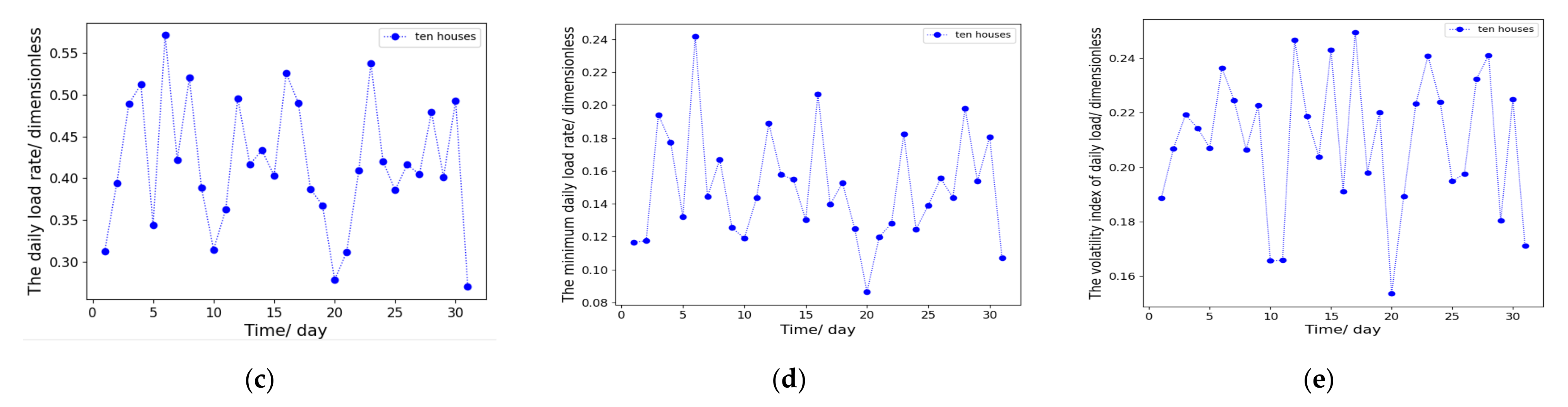
2.2. Characteristic Analysis of Residential Electric Loads

Among the public datasets about residential electric load, three datasets are used widely in the papers. They include the data from Smart Grid Smart City (SGSC) project in Australia [39], the data from the Smart Metering project in Ireland [40], and the data from the Smart-star project in the USA [41]. The SGSC project comprises historical electric load data of 10,000 households recorded from 2012 to the 2014 under a sampling interval of 30 min, while the load data of about 4000 households from 2009 to 2010 was recorded under the same sampling interval in the Smart Metering project. Unlike the abovementioned datasets, the electric load data and external factors are detailed and recorded for about 400 households from 2013 to 2016 in the Smart-star project, and the sampling interval reaches 1 min for several individuals.
Due to the good readability and complete continuity of the recorded data, the set from the SGSC project will be used in our research after the comparison. Firstly, the characteristic of a single-unit residential electric load is analyzed over a long period of time. Secondly, the load characteristics of different units are analyzed and compared with each other. Thirdly, the difference between a single-unit load and the aggregated load of multiple units is detailed analyzed, and the results will be used for the following load prediction method in this paper.

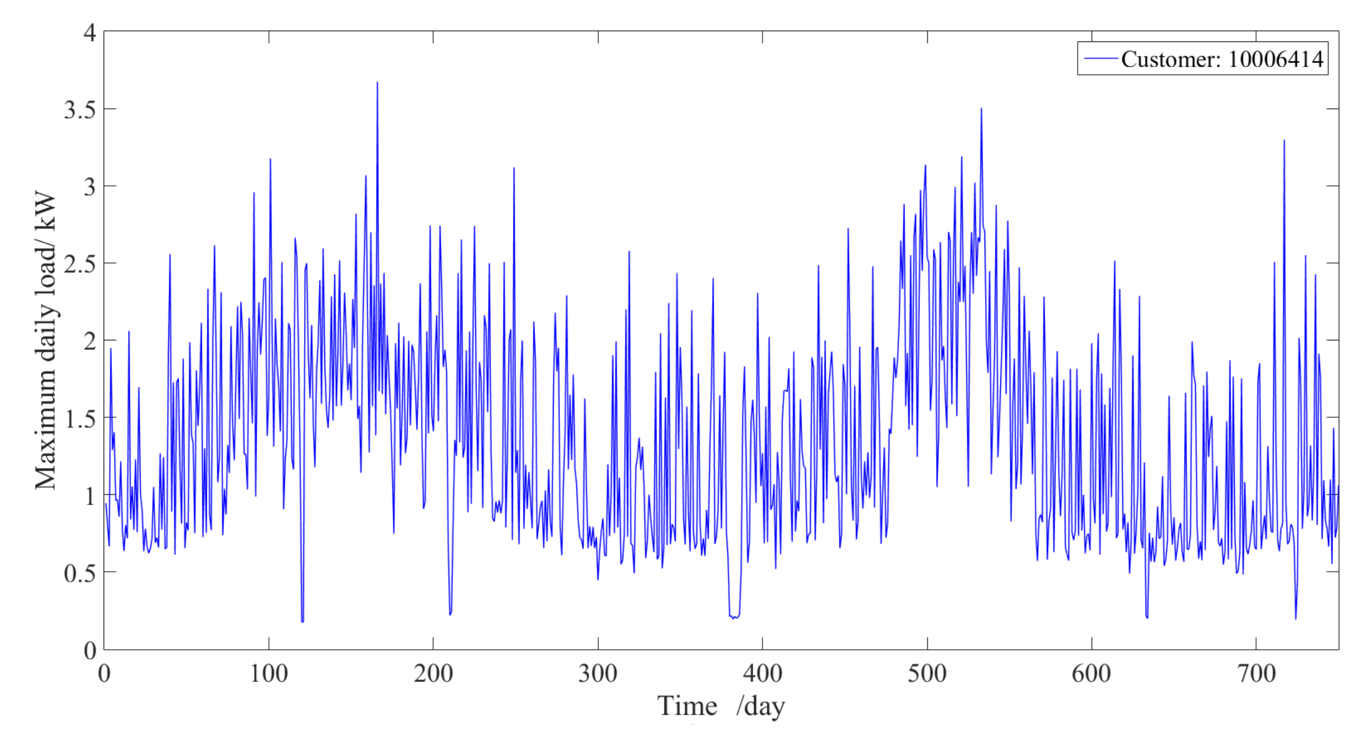
2.2.1. Electric Load Characteristics of a Single Unit

As an example, take the residential electric load of the customer numbered as 10006414. The corresponding recorded power consumption data from February 2012 to March 2014 is selected as sample data. The indicators of the selected data are calculated to illustrate the load characteristics.
The obtained maximum daily loads of the customer with number 10006414 for 750 consecutive days are shown in Figure 1. Statistical analysis has been performed to obtain the distribution of the maximum daily loads. The most probable maximum daily load is in the range of (0.5 kW, 1.0 kW), which accounts for 37.5% of the total 750 days. The proportion of maximum daily load with the range of (1.0 kW, 1.5 kW), 20.0%, is similar to that with the range of (1.5 kW, 2.0 kW), which equals 21.6%. The proportions of maximum daily loads with the range of (2.0 kW, 2.5 kW) and the range of (2.5 kW, 3.0 kW) equal 11.2% and 5.9%, respectively. In addition, the maximum daily load changes with the seasons. For example, as shown in Figure 1, the values of maximum daily loads from April to October are bigger than those from November to March.
Other characteristics of residential load for the customer with number 10006414 have also been analyzed. The other corresponding quantitative indicators of residential electric loads for these 750 days are also analyzed and given as follows.
The mean daily load of customer 10006414 is mainly located in the range of (0.2 kW, 0.4 kW), and the corresponding proportion equals 63.2%. In the meantime, the mean daily load increased significantly in the period from the middle of May to the beginning of August. The proportions of mean daily loads with the range of (0.4 kW, 0.6 kW) and the range of (0.6 kW, 0.8 kW) equal 21.9% and 7.9%, respectively.
The mean loading rate mainly varies in the range of 0.2 to 0.4. It is much less than the loading rate of a provincial region, which usually equals 0.8. These results show that the residential load is more volatile than the regional load. Furthermore, the minimum loading rate is in the range of 0.05 to 0.15. In other words, the peak–valley difference of the residential load is very big, and it is far below that of industrial loads. The corresponding daily volatility index is in the range of 0.15 to 0.3. The high volatility and big peak–valley difference of residential load bring an enormous challenge for the short-term residential load prediction.

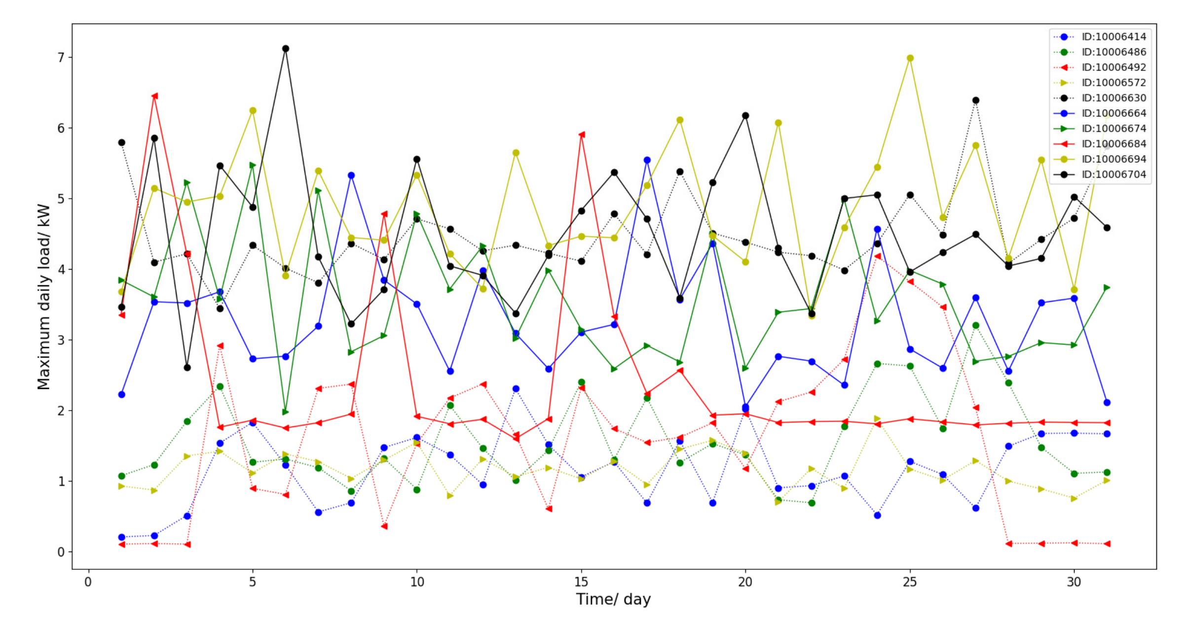
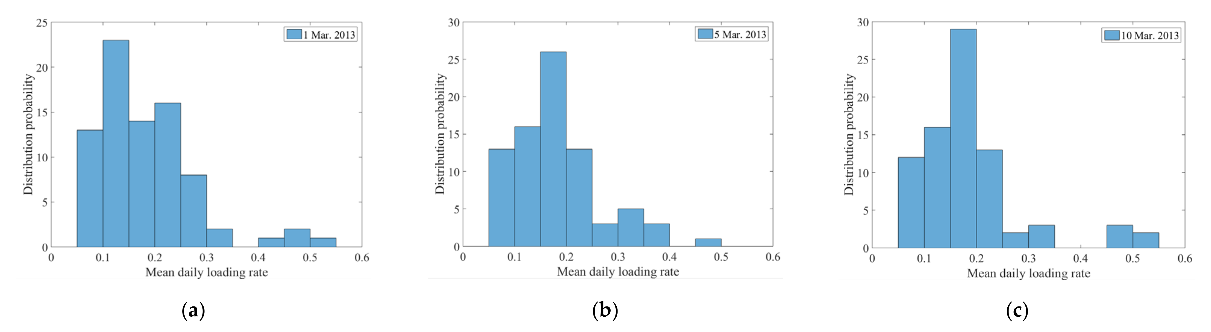
2.2.2. Electric Load Characteristics of Different Units

Ten households are randomly selected from the SGSC set data, and the corresponding load characteristics are analyzed and compared with each other based on the historical data in March 2013.
The maximum daily loads of the selected ten units are shown in Figure 2. The results show that no noteworthy associations exist between two maximum daily loads curves. For example, the maximum value of the maximum daily loads of customer 10006414 appears on 13 March and equals 2.306 kW, while the minimum value appears on 1 March and equals only 0.206 kW. The maximum value of the maximum daily loads of customer 10006704 appears on 6 March and equals 7.126 kW, while the minimum value appears on 3 March and equals 2.608 kW. There are obvious differences between the maximum daily loads of customer 10006414 and that of customer 10006704.
The mean daily loads and the daily volatility indicators of these ten selected units are also analyzed, and some quantitative indicators are given in Table 1 for intuitive and clear comparison.
The mean daily load analysis results show that some customers consume similar daily electric quantities among these days, and some customers are different. For example, the mean daily loads of customer 10006414 fluctuate within a small range of (0.2 kW, 0.4 kW), and the mean daily loads of customer 10006572 also fluctuate within a small range of (0.4 kW, 0.6 kW). Unlike these two customers, the mean daily load of customer 10006684 varies on a large scale. The values fluctuate sharply from 2 kW to 6.5 kW on 3 March, 9 March and 15 March, while the values remain in the range of (1.8 kW, 1.9 kW).
Compared to the irregular patterns of residential loads, the daily volatility indicators of the selected ten customers are within the same range, located from 0.15 to 0.25. However, further analysis indicates that the daily volatility index variation curves of any two households are different. These results are caused by the similar household appliances and different working processes in these selected units.
The electric loads of eighty selected households are used to form the distribution probability of mean daily loading rates, and the distributions on three selected days are shown in Figure 3. For the same eighty households, the distribution probability of mean daily loading rates is different on 1 March, 5 March and 10 March in 2013. On 1 March, the maximum probability of the mean daily loading rates appears in the range of (0.1 kW, 0.15 kW), while the maximum probability of the rates appears in the range of (0.15 kW, 0.2 kW). In the meantime, the mean daily loading rates of these selected eighty households are distributed in a wide range, especially in the range of (0.05 kW, 0.4 kW).

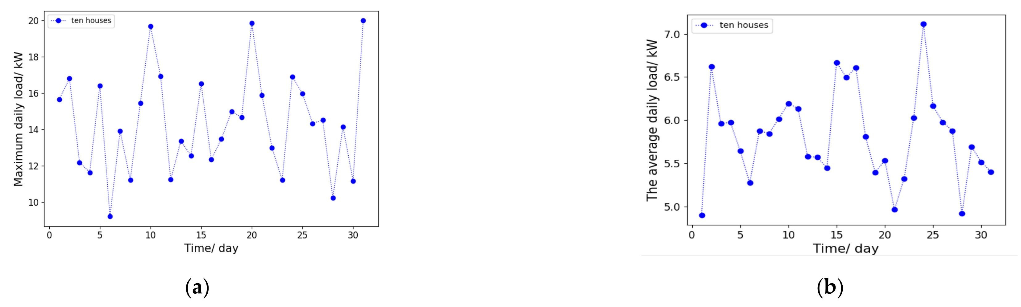
2.2.3. Electric Load Characteristics of a Single Unit and Total Loads of Multiple Units

The abovementioned analysis results show that the electric load of a single unit has weak regularity. If the traditional load prediction methods are applied for the load forecasting of a single unit, a big forecasting error would inevitably appear. Based on the field data and historical experience, the daily volatility index of the total electric load of a whole region is very small because the load fluctuations of all units balance themselves out. With the increase in households in the region, the pattern of the total electric load becomes more and more stable, but too many residents in one region would exceed the scale limit of the microgrid, and then reduce the operational flexibility of the microgrid.
Quantitative indicators of the total electric load of the abovementioned selected ten households are analyzed and shown in Figure 4. Furthermore, another ten households are added to the cluster, and the indicators of the total electric load of twenty households are analyzed. The quantitative indicators of these total residential electric loads are also listed in Table 2.
There is some regular pattern in the total power consumption of the selected ten households. As shown in Figure 4a, the maximum daily loads of the total load of the ten households appears as local minimums on 6 March, 12 March, 16 March, 23 March and 20 March, and the corresponding values equal 9.232 kW, 11.252 kW, 12.3256 kW, 11.222 kW, and 11.178 kW, respectively. The maximum daily loads of the total load of the ten households appear as local maximums on 10 March and 20 March, and the corresponding values equal 19.674 kW and 19.866 kW. The maximum daily loads of the total load contain specific periodic components expect for some fluctuations between 6 March and 16 March. The maximum daily loads of the total load of the twenty households have more stable regularity. More precisely, the first local minimum of maximum daily loads of the total load appears on 6 March, which equals 12.226 kW. Then, the maximum daily load of the total load increases to the first local maximum value, occurring on 10 March, which equals 23.728 kW. Subsequently, the maximum daily load of the total load decreases to the second local minimum value, occurring on 14 March, which equals 14.462 kW. The maximum daily loads of the total load vary with the same periodic pattern in the following days.
Moreover, the maximum value of maximum daily loads for the total load of the ten households in March 2013 equals 20 kW, while the maximum value of maximum daily loads for the total load of the twenty households only equals 25 KW. In the meantime, the maximum value of maximum daily loads for a single household with number 10006704 among these selected twenty households unexpectedly reaches 7 kW on 6 March. Therefore, the maximum daily load does not increase linearly with the increase in households in a small area during a period of time. The optimal aggregation of residential loads would smooth the electric load under a small enough region to ensure the flexibility of the energy management.
As shown in Figure 4b, the mean daily loads of the total load of the ten households fluctuate within the range of (5 kW, 6.5 kW), and some outlier data exist in the curve. For example, the mean daily load of the total load of the ten households on 24 March equals 7.1 kW. For the twenty households, the mean daily loads of the total load vary within the range of (8 kW, 11 kW), and only one point does not locate in this range, which appears on 2 March and equals 12.1 kW. The mean daily load becomes more regular with the total number of houses increasing.
The mean daily loading rates of the total load of the selected ten households are analyzed in March 2013, and the results show that these rates are in the range of (0.3, 0.55). The results also show that the mean daily loading rates of the total load of the selected twenty households are in the range of (0.4, 0.65). In contrast with these aggregated loads, the mean daily loading rates of a single household are located in the range of (0.1, 0.3), which is discussed in Section 2.2.2. This comparison result demonstrates that the total load is tending towards stability with the total number of houses increasing. The analysis results of daily volatility indexes are also used to verify this result again. Compared with the daily volatility indexes of a single household within the range of (0.15, 0.25), the daily volatility indexes of the total load of the ten selected households are in the range of (0.16, 0.24), and the indexes of the twenty selected households are in the range of (0.15, 0.23). This result shows that the daily volatility indexes reduce slightly when the total number of households increases.
Compared with the quantitative indicators of a single household given in Table 1 and those of the aggregated load given in Table 2, the residential load of a single household has high volatility, strong randomness, and weak regularity. With the increase in the total number of households, the total aggregated load becomes more and more stable, and the cyclical pattern of the aggregated load becomes more and more distinct. Therefore, in our proposed short-term residential load forecasting method, the optimal number of households would be selected, and the total aggregated residential load of the selected households is used separately for prediction.

3. A Novel Short-Term Residential Electric Load Forecasting Method

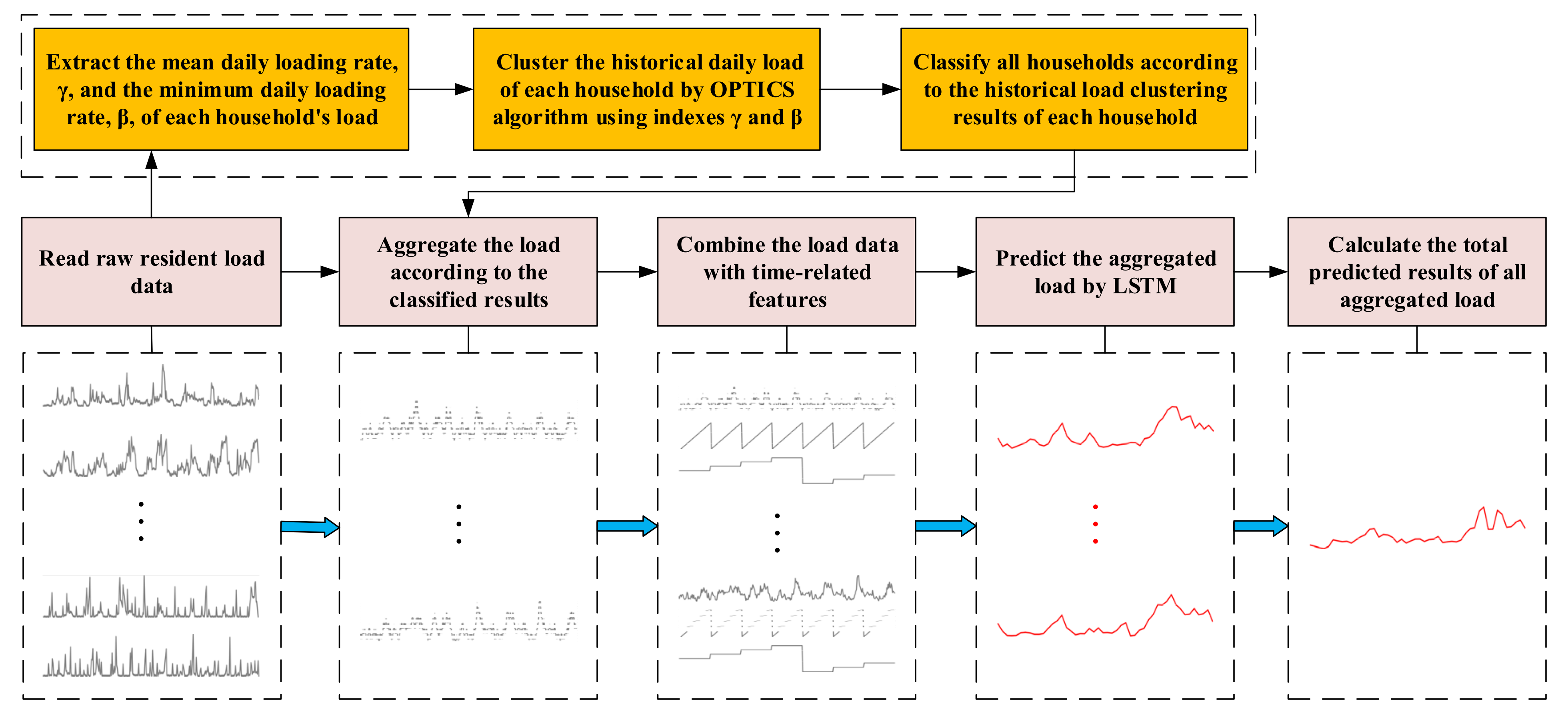
3.1. Basic Principle of Our Proposed Method

Short-term residential electric load forecasting is used to predict the power consumption in the next hours. In our proposed method, the aggregated load of multiple households is used, instead of that of a single household. The total number of households is determined by the minimum households when the short-term prediction result of the corresponding aggregated load meets the precision requirements. The detailed residential load prediction process of our proposed method is shown in Figure 5.
We would extract the mean daily load rate, γ, and the minimum daily load rate, β, from the raw residential load data first. Then, the historical daily load of each household is clustered by the ordering points to identify the clustering structure (OPTICS) algorithm, using indexes γ and β. Thirdly, the residential load would be aggregated adaptively according to the classified results of all households. The basic principle of household classification is that the households with the same number of clusters for historical data would be classified into one category. Additionally, the households with a number of clusters greater than two are all classified into one category. The aggregated load data and the corresponding time-related features are used as the input parameters of the long short-term memory (LSTM)-based forecasting model. Finally, the total load predicted results are obtained using all selected and aggregated load forecasting results.

3.2. Optimal Number of Total Aggregated Households

As discussed in Section 2.2, the pattern of the total electric load becomes more and more stable with the increase in the total number of aggregated households. The total aggregated residential loads would smooth the electric load under a small enough region to ensure the flexibility of the energy management. The randomness and fluctuation of the residential load are determined by the human life routine and home appliances; thus, it is related to the city in which these households are located.
In this paper, we use a typical LSTM-based load forecasting method to identify the optimal number of total aggregated households. The relationship between the prediction MAPE and the number of total aggregated households can be obtained through a great deal of load prediction processes under different numbers of randomly selected households. The optimal number is identified as the minimum number of households when the MAPE meets the requirement of the microgrid dispatch.

3.3. Adaptive Density-Based Spatial Clustering Algorithm for the Residential Load

The analysis results in Section 2.2 show that obvious differences exist in the power consumption patterns of different households. To enhance the regularity of the aggregated residential load further, the households with similar patterns in the optimally selected households will be clustered as one group. Then, the corresponding load of each group is used separately for prediction. In our proposed method, the OPTICS algorithm will be used to identify households with similar patterns.
Typical clustering algorithms include K-means, density-based spatial clustering of applications with noise (DBSCAN), and OPTICS. The comparison results among these algorithms are given in Table 3.
Due to the high volatility and strong randomness of residential load, it is not possible to identify the clustering number of the selected households in advance. In the meantime, some daily loads are irregular and should be regarded as outliers. Although there are some other extensions of K-means algorithms to select a proper cluster number or remove the outliers automatically [42,43], the improved K-means algorithms would be too complicated to find a proper cluster number and remove the outliers simultaneously. Therefore, the K-means algorithm is not suitable for our proposed method. Two parameters of the DBSCAN algorithm directly affect the reasonability of the clustering results, including the distance from a neighborhood point to a defined core point and the minimum number of samples in a cluster, but the selection of these two parameters has no paradigm. Improperly selected parameters would significantly reduce the effectiveness of the DBSCAN algorithm. In contrast, a variable neighborhood radius is used in OPTICS algorithm to avoid the influence of improper parameters on the clustering result. The samples can be clustered adaptively based on the distribution density. In this paper, the OPTICS algorithm is used to realize load clustering.
The detailed residential load clustering process is given as follows.
Step 1: The quantitative indicators of all residential electric loads in the objective area are analyzed and used for the distance calculation in the clustering algorithm. In our proposed method, the mean daily loading rate, γ, and the minimum daily loading rate, β, are selected as the key parameters for load clustering. These two parameters of ith historical daily load of the kth household are represented by γk,i and βk,i, respectively. The distance between the quantitative indexes of ith day and jth day of the kth household is represented by dk,i,j, and can be expressed by d k , i , j = γ k , i γ k , j 2 + β k , i β k , j 2 .
Step 2: The historical loads of the kth household in the past D days are clustered by the OPTICS algorithm. The detailed process is illustrated as follows, which includes Algorithms 1 and 2. These historical loads of the kth household would be clustered as NCk classes. The pth class includes Np days, which are denoted as Dk,p,1, Dk,p,2,…, Dk,p,Np.
Algorithm 1 The Clustering Subprocedure 1
input: D: total number of historical days, dk,i,j: distance between the ith day and jth day of the kth household, MinPts: minimum samples in the neighborhood area, Ω: set of core samples, N: size of the set Ω, cd(o): the core distance of element o, rd(j, o): reachable distance from element j to element o.
output: results queue M.
1 foreach item  o Ω  do
2 Mark item o and put it into results queue M
3 Calculate the reachable distance of any element j ( d k , o , j d s e t ):
  r d j , o = max c d o , d k , o , j
4 The unmarked elements belonging to the neighborhood area of o are sorted in ascending order. And put the elements into seeds queue P.
5 If p = , then jump to the line 1 and move to the next element.
6 If p , foreach item q p , mark item q and put it into results queue M.
7  If q Ω , the unmarked elements belonging to the neighborhood area of q are put into seeds queue P. And calculate the reachable distance of any elements belonging to queue P.
8  If q Ω , do nothing
9 end
10 end
Algorithm 2 The Clustering Subprocedure 2
input: M: results queue, dset: distance set value, ρset: set value for noise point treatment.
output: NCk subsets after the clustering process
1 foreach item  s M  do
2 If r d s , o d s e t , item s is assigned to the current cluster
3  If r d s , o > d s e t   &   c d s ρ s e t , item s is identified as an outlier
4  If r d s , o > d s e t   &   c d s < ρ s e t , item s is assigned to another cluster
5 end
Step 3: All households in the region are aggregated into several groups based on the clustering results in step 2. The detailed process is given as follows.
Step 3.1: If the number of clusters for kth household equals that for jth household, the kth household and jth household would be aggregated as one group. All households would be divided into NH classes, and the number of households in the mth class is represented by Nm.
Step 3.2: If the number of households in the mth class exceeds the threshold Nset, the mth class should be divided into small groups again. The number of clusters for any household in the mth class is represented by U. For any household b, the corresponding cluster id is sorted in descending order according to the days contained in the cluster. The historical days in the qth cluster id of household b is represented by set N(b,q), and the elements of N(b,q) are represented by Db,q,1, Db,q,2,…, Db,q,Nq. The household x and household y in the mth class would be aggregated into one group if the following criteria were met.
(1) k1 × [|N(y,1)| + |N(y,2)|] ≤ |N(x,1)| + |N(x,2)| ≤ k2 × [|N(y,1)| + |N(y,2)|]. Generally, k1 is set as 0.7 and k2 is set as 1.3.
(2) |N(x,1) ∩ N(y,1)| ≥ k3 × |N(x,1) N(y,1)|. Generally, k3 is set as 0.25.
(3) |N(x,2) ∩ N(y,2)| ≥ k4 × |N(x,2) N(y,2)|. Generally, k4 is set as 0.15.
According to the abovementioned three steps, residential loads in the predicted area can be clustered and aggregated adaptively. The results would be used as the input of LSTM to realize short-term residential load forecasting.

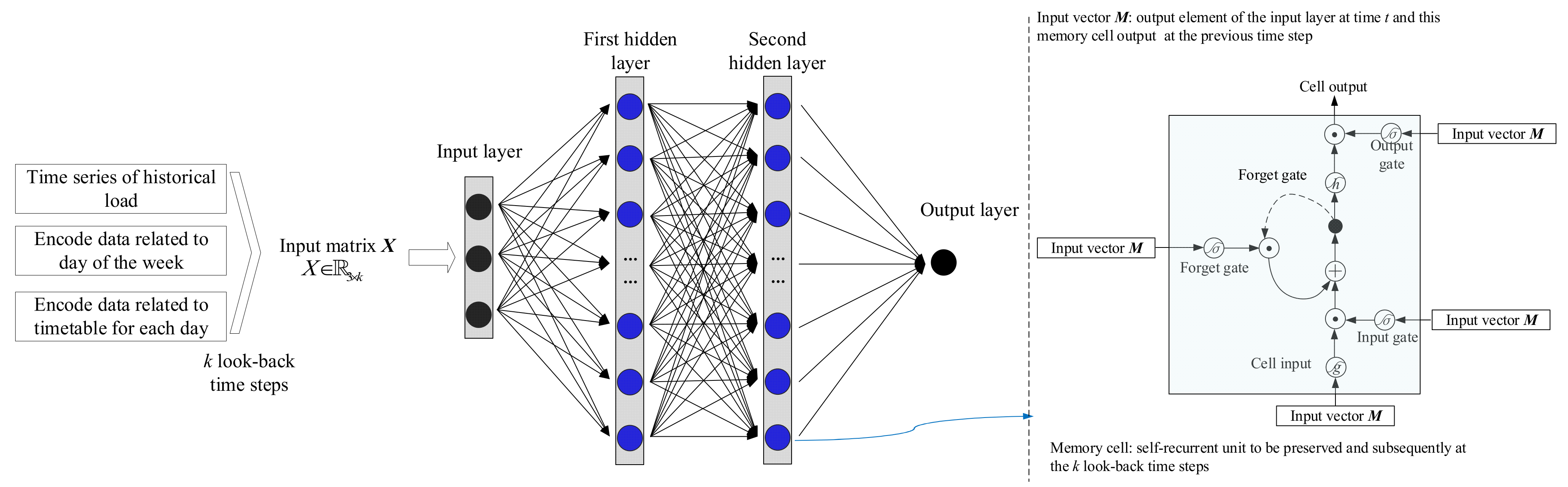
3.4. LSTM-Based Short-Term Data Prediction for Residential Load

LSTM is one kind of recurrent neural network (RNN). In LSTM, the cell state is added to the hidden layer, and the forget gate parameter is used to update the cell state. Therefore, cell state can be further used to identify the signals which need to be abandoned and the signals which are required to be reserved in the next step. This characteristic can be applied to maintain the dependency relationship in the long time series without vanishing and exploding gradients problems. The inherited ability to maintain historical data regularity can improve prediction accuracy in the future. Therefore, LSTM is selected as the deep learning algorithm to predict the short-term load in the next hours in our proposed method.
The LSTM-based short-term data prediction process for residential load is shown in Figure 6. In our method, a proper K look-back time step is defined to select the length of time series of historical load as the input data. In the meantime, time-related feature data are also extracted and used to form the input matrix.
(a)
The time series of historical load under selected K look-back time step, which is represented by E = {et−K, et−K+1, …, et−2, et−1};
(b)
The daily load data are related to the timetable each day. Hence, the time t in each day is encoded into t/dx according to the load sampling interval dx;
(c)
The pattern of historical data is related to human life routine, which is usually inextricably linked to the day of the week. Hence, the sorted number of days of the week related to the historical data is encoded into 0 to 6.
The input matrix would be preprocessed to avoid the influence of different dimensions of data and improve the convergence rate by the min–max normalization. The constructed input matrix X 3 × k is then used as the input data of our proposed LSTM-based forecasting model. The constructed load forecasting LSTM network consists of one input layer, two hidden layers, and one output layer. The input layer contains three cells, and each hidden layer contains twenty memory cells. Each memory cell is a self-recurrent unit, and it is preserved subsequently at the k look-back time steps. The input vector M for the memory cell consists of the output element of the input layer at time t and this memory cell output at the previous time step.
The residential load data of similar days at the same time are relevant to the load value of the prediction day at the prediction time, as well as the load data at the previous time window. Therefore, the look-back time steps should be set as the integral multiple of the total sampling number, 24 h/dx, of a whole day.

4. Simulation and Results Discussion

4.1. Experimental Datasets and Criteria in the Proposed Load Prediction Process

In this paper, the residential load set from the SGSC project is used in our short-term residential load prediction. The recorded residential load of 50, 100, 150, and 200 randomly selected households is used to verify our proposed method. The corresponding period of time is from 1 March 2013 to 31 March 2013. These load data are divided into two subsets, including the training set and test set. In the training set, the data from 1 March to 24 March of 1152 samples are selected to train the constructed LSTM network. Furthermore, 336 load samples from 25 March to 31 March are used to test our proposed short-term load forecasting method.
In the forecasting method, several parameters, especially the hyperparameters of the LSTM network, are predefined according to our rich experience in load forecasting.
a)
Thirty-one history days are used in our experimental datasets, hence, the minimum number of points in the neighbors, MinPts, is set as five in the OPTICS clustering algorithm.
b)
The short-term load forecasting result is used for microgrid power dispatch. Hence, the high computational efficiency is needed in our scenario. The learning rate is set as 0.01 initially, with an Adam optimizer to reduce the LSTM network learning time. In the meantime, the number of iterations is set as 150 to avoid continuous oscillation. To effectively evaluate the load forecasting result, MAPE of the prediction load is used in the cost function.
c)
The sampling time interval of the historical load data is 30 min. Hence, there are 48 samples in a whole day. The look-back time step of the LSTM network is set as 48; therefore, the load at the same time of the previous day and the load before the prediction time can be both used to reveal the forecasting load value.
d)
The rolling load prediction strategy is adopted for the short-term residential load forecasting in this paper. In our following experiments, the constructed LSTM network outputs one prediction result after each prediction process without loss of generality.

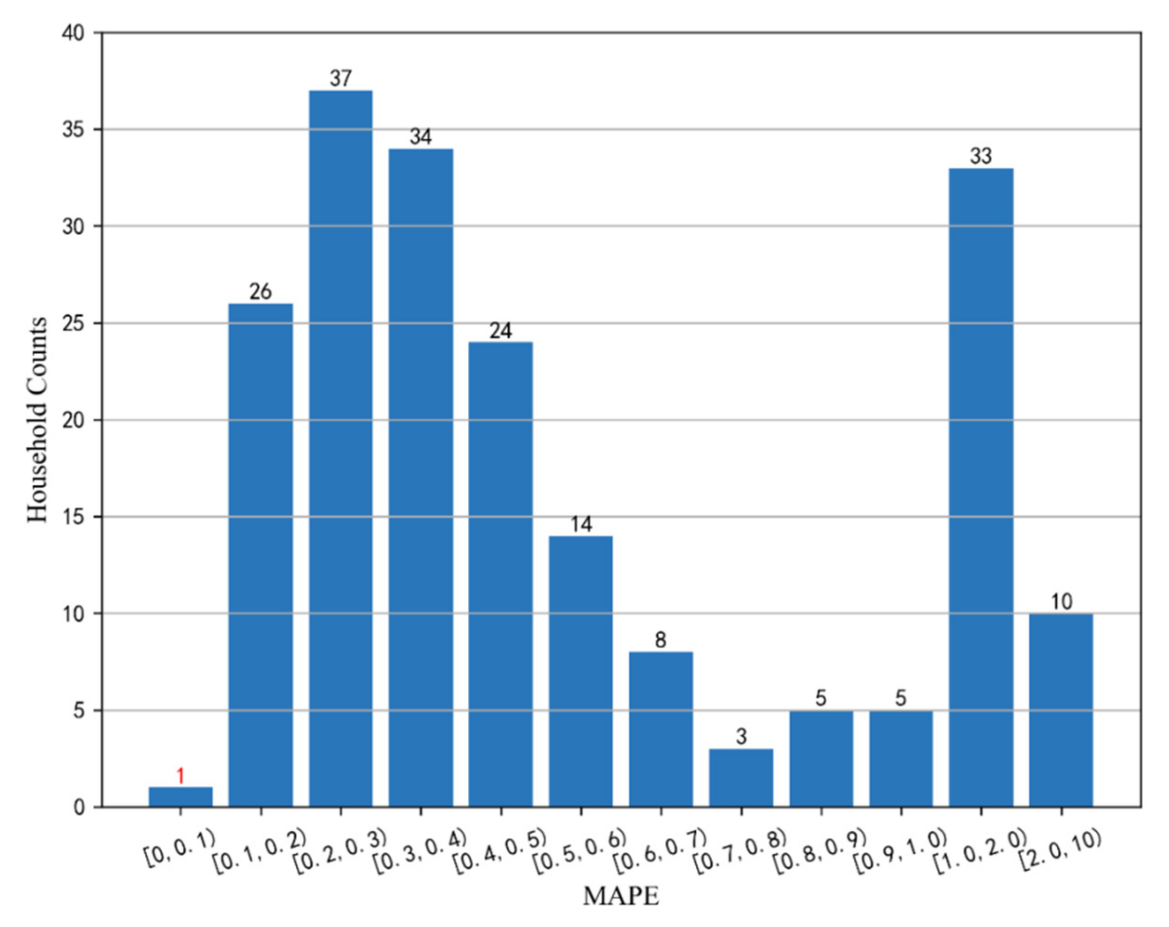
4.2. Short-Term Residential Load Forecasting Results of a Single Household

The short-term load forecasting tests are carried out for each household by our proposed LSTM-based forecasting method. The MAPE values of 48 forecasting results on 31 March are calculated for each of the 200 selected households. The distribution of the corresponding 200 MAPE values is shown in Figure 7.
As shown in Figure 7, the distribution of MAPE values on 31 March for the selected 200 households is analyzed according to the twelve divided ranges. The vertical axis represents the total number of residential households within the corresponding range. Only one MAPE value is below 10% among these 200 households, while the MAPE values of other households are greater than 10%. Notably, ten MAPE values are even greater than 200%. The vast majority of individual forecasting errors are greater than the average MAPE values of 200 households, which equals 74.6%. This result shows that the forecasting error of any individual forecast has high variability, and the short-term load prediction accuracy of a single household cannot meet the requirements of home energy management.

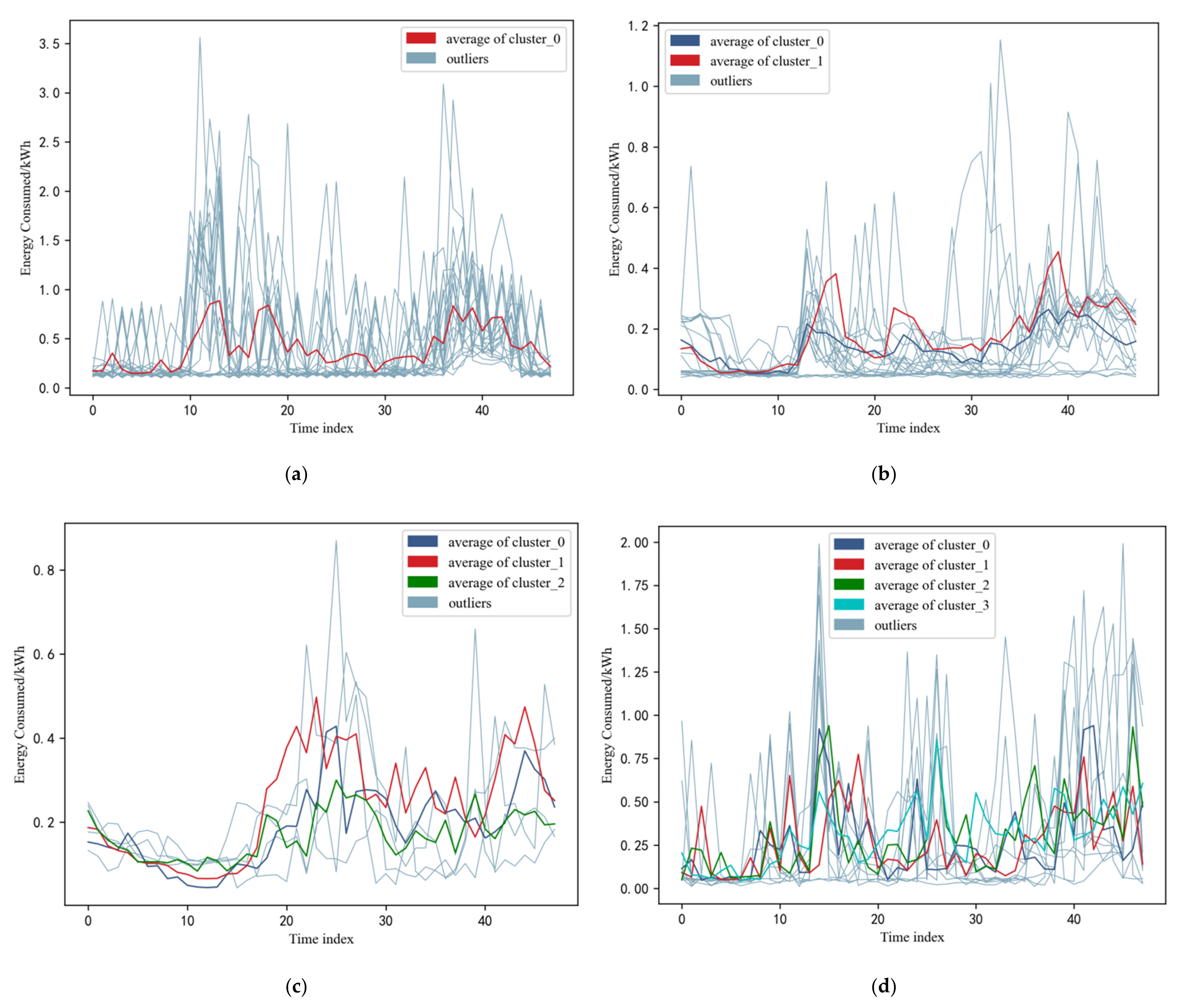
4.3. Results of Residential Load Clustering

The minimum daily loading rate and the mean daily loading rate mentioned in Section 2.2 are used as the key parameters of daily load clustering for individual customers. The clustering results of daily load curves of the selected 200 households can be obtained by the OPTICS algorithm. The total number of clusters for each household will be used for the adaptive load aggregation. The clustering results for some selected households in March 2013 are shown in Figure 8, and the clustering results are detailed given in Table 4.
As shown in Figure 8, the average series of each cluster is plotted with bold lines. Figure 8a shows the historical load curves clustering results of the customer number 10006704. The total number of clusters equals 1. This means that the customer has only one pattern of power consumption, and the peak electricity consumption is concentrated in the morning and evening hours. Figure 8b shows that the total number of clusters equals 2 for the customer number 10006414. This indicates that there are two main forms of electricity consumption for this household. In the one power consumption pattern, the peaks concentrated in the morning and evening hours. In the other pattern, electricity is consumed throughout the whole day. Figure 8c,d represent the scenarios where the total number of clusters is 3 and 4, respectively. Figure 8c can reflect the electricity consumption characteristics of residents with less electricity consumption before 10:00 a.m. and with three main electricity consumption behaviors, while Figure 8d indicates that the household has four electricity consumption behaviors. It indicates that the residents have stronger regularity of living electricity consumption in these two scenarios.
As given in Table 4, when the total number of clusters equals 1, the number of outliers is 21, and when the number of clusters is 2, the number of outliers is 18. The number of outliers accounts for 2/3 of the total days, which shows the poor regularity of electricity consumption for these households. When the number of clusters equals 3 or 4, the number of outliers is less than 1/3 of the total days, and the number of clusters is evenly distributed. This indicates that the electricity load has a strong regularity, and also reflects the reasonableness of aggregating households with more than three clusters into one category, because they represent households with regular electricity consumption. The clustering results of fifty randomly selected households show that the users with two clusters reach 50%, while the users with four clusters only account for a small percentage, 2%. This result also verifies that it is reasonable for households with more than three clusters to be aggregated into one category.
Therefore, in this paper, households with the same number of clusters were aggregated into one category when the clusters are below three and all the households with more than three clusters were aggregated into one category. Groups of 50, 100, 150, and 200 customers are randomly selected and clustering analysis is processed based on the historical load data, and the final categories of the households are shown in the following Table 5.
It can be seen from Table 5 that the number of households of category 1 always accounts for about 1/5 of the total number of households. The number of households in category 2 always accounts for about 1/2 of the total number of households. It indicates that the vast majority of households have certain electricity consumption patterns. Hence, it is necessary to forecast the load of the households with poor and strong electricity consumption patterns separately in our proposed method.

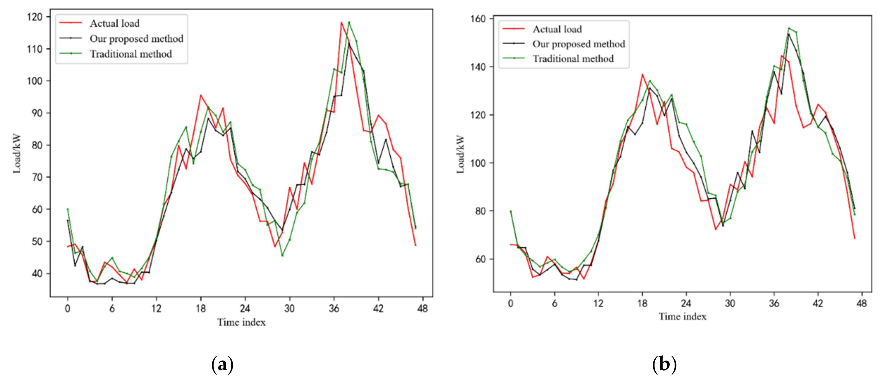
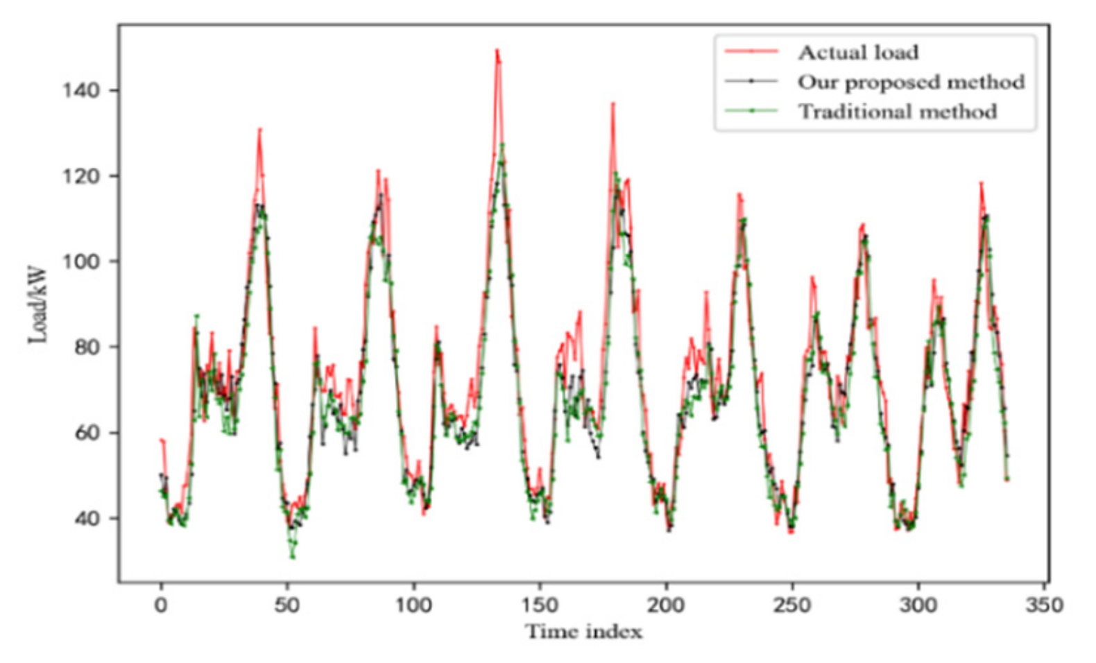
4.4. Results of Short-Term Residential Load Forecasting

Based on the aggregation results of 50, 100, 150, and 200 households, the load forecasting for each aggregation category was performed separately, and the MAPEs of the summing forecasting load are given in Table 6.
As given in Table 6, the forecasting error of the total load prediction, as well as the adaptive aggregated load prediction, decreases sharply with the increase in the total number of households. In the meantime, the MAPE of the adaptive aggregated load prediction is always lower than that of total load prediction from 50 to 200 households. This result confirms the effectiveness of the proposed method. For our proposed method, 50 households are predicted with a MAPE of 14.3% and 100 households are predicted with a MAPE of 10.2%. When the number of households reaches 150, the MAPE of both the traditional method and our proposed method are both below 0.1, which meets the requirement of load forecasting accuracy when dispatching a microgrid. In general, for 150 households, the load forecasting results can achieve the accuracy requirement, and the number of households is not too large. Therefore, 150 would be an ideal number of households to construct a microgrid.
The detailed forecasting results at 48 points on 31 March for 150 and 200 households are shown in Figure 9. We can find that the fitting effect of our proposed method is significantly better than traditional methods. This verifies the advantage of our proposed method. The prediction accuracy of 200 households is significantly better than that of 150 households, which meets the analysis results expressed in the previous section. In general, the prediction accuracy of 150 households meets the requirement of prediction accuracy for microgrid construction.
To further verify the effectiveness of our proposed method, the data from 1 March to 24 March, totaling 1152 samples, are selected to train the constructed LSTM network. Additionally, 336 load data samples from March 25 to 31 March are used to test our proposed short-term load forecasting method. The forecast results for 150 households are shown in Figure 10.
As shown in Figure 10, the short-term load forecasting of our proposed method is always better than that of traditional methods during the whole week. The average MAPE of our proposed method during the week is 8.2%, while the average MAPE of the traditional method is 8.9%. A large number of forecasting results in this paper confirm the effectiveness of the proposed method. However, when the peak–valley value of the load is predicted, the overall effect of load forecasting is unsatisfactory. The reason is that various hyperparameters are not optimized in our method. This problem would be solved in our future work.

4.5. Sensitivity of Look-Back Time Steps of the LSTM Network

In our proposed method, the look-back time step, k, is selected as 48 to reveal the relationship between the historical load data and the prediction load. In this section, different look-back time steps are selected to analyze the load forecasting accuracy. The MAPE of the prediction results for 6 and 48 time steps in the LSTM network on 31 March are given in Table 7.
As given in Table 7, for the households with the number of 50, 100, and 150, the MAPE of prediction results on 31 March is different when different look-back time steps are selected in the load forecasting process. For the households with the number of 50, the MAPE reaches 14.3% when the time step equals 48, while the MAPE reaches 18.3% when the time step equals 6. The MAPE for the 48 look-back time steps is lower than that for the 6 look-back time steps. Similar results can be conducted for the households with the number of 100, 150, and 200. The reason is that the residential load at the prediction time is usually related to the load at the same time on the previous day.

4.6. Comparison with Traditional Methods

Two other traditional prediction methods, SVR-based and BPNN-based load forecasting, are used to compare with our proposed method. The setting parameters for these two traditional load forecasting methods are given in Table 8. The comparison results with traditional methods for the 150 selected households are given in Table 9. The MAPEs of the short-term load forecasting results on 31 March for three methods are calculated and given in this table. To verify the advantages of our proposed method clearly, the load forecasting results are obtained based on two load processing methods. In the first prediction process, the total load data is directly used as the input parameters of the artificial intelligence algorithms. In the second prediction process, the aggregated load data in Section 4.3 will be used separately as the input parameters of the forecasting model. The MAPE values in Table 9 represent the final predicted result errors of the summing aggregated load forecasting results. The content has been revised to avoid misunderstandings of our comparison results.
The comparison results show that our proposed method has the best load forecasting results whether the residential load is aggregated or not. When the total load is forecasted directly, the MAPE of our proposed only equals 9.1%, which is lower than traditional methods. When the aggregated load is forecasted separately, the MAPE of our proposed method equals 8.3%, while the MAPE of the SVR-based method equals 11.2% and the MAPE of the BPNN-based method equals 10.2%. In all cases, our proposed method gets the best MAPE value.
The load forecasting results vary under multiple runs for our LSTM-based method or the BPNN-based method. The reason should be the random initialization of weights of trainable layers or parameters in the artificial intelligence models. We select the average of several runs in the comparison. We run the constructed LSTM and BPNN models by fifty runs. In each run, the aggregated load data in Section 4.3 will be used separately as the input parameters of the forecasting model. The MAPE values represent the final predicted 48 results errors of the summing aggregated load forecasting results. The average and variance of the MAPE values for the LSTM-based method are 8.19% and 6.13 × 10⁻⁶, respectively, while the average and variance of the MAPE values for the BPNN-based method are 10.12% and 2.56 × 10⁻⁵, respectively. A Student t-test showed that the difference was statistically significant, where t = −24.22 and p = 0.000. Therefore, the results of our method are better than those from the traditional algorithms.
We have recorded the computational time of our proposed method and the traditional methods to make the comparison more comprehensive. Each run of the residential load forecasting includes the training process and 48 prediction processes. The program runs on GPU (Graphics Processing Units), whose type is NVIDIA GeForce GTX 1650. The results show that the computational time of our proposed method is around ten minutes, while the computational time of BPNN-based and SVR-based algorithms is around one second. The training time of the LSTM-based model is much longer than that of traditional methods due to the complicated structure of the LSTM-based model. It is worth noting that the computational time of our proposed method is much shorter than half an hour. Therefore, our proposed method can be sufficiently used for hourly load forecasting in microgrid dispatching.

5. Conclusions

A novel short-term residential electric load forecasting method based on adaptive load aggregation and deep learning algorithms is proposed and discussed in this paper. An adaptive load aggregation method is proposed based on the number of clusters of historical load data of each household. Households with the same number of clusters are aggregated into one category when the cluster number is below three. All the households with more than three clusters were aggregated into one category. The LSTM-based network with proper look-back time steps is used to forecast the total aggregated load of each category. The look-back time steps are set as the ratio of 24 h to the load sampling interval. This can take into account the load at the same time on the previous day and the load before the prediction time because of the good performance of the LSTM network at storing and accessing long-term information. A large number of experiments using the monitoring load data from the SGSC project show that 150 households are the proper scale to construct a microgrid, because the corresponding MAPE of load prediction for 150 households is less than 10% and meets the requirement of the microgrid dispatch. Our proposed method can significantly improve the load forecasting accuracy for the residential load with high volatility, strong randomness, and weak regularity, and it is very important in microgrid planning and operation.

Author Contributions

Conceptualization, J.T. and T.H.; methodology, J.T. and R.F.; validation, J.L., G.G. and J.T.; formal analysis, J.T.; investigation, T.H. and R.F.; writing—original draft preparation, J.T., G.G. and J.L.; writing—review and editing, J.T.; project administration, T.H. and R.F.; funding acquisition, D.Y. and W.Z. All authors have read and agreed to the published version of the manuscript.

Funding

This research was funded by State Grid Hubei Electric Power Company, grant number 52153820000J.

Institutional Review Board Statement

Not applicable.

Informed Consent Statement

Not applicable.

Data Availability Statement

Not applicable.

Conflicts of Interest

The authors declare no conflict of interest.

References

  1. Koo, C.; Hong, T.; Lee, M.; Kim, J. An integrated multi-objective optimization model for determining the optimal solution in implementing the rooftop photovoltaic system. Renew. Sustain. Energy Rev. 2016, 57, 822–837. [Google Scholar] [CrossRef]
  2. Ondeck, A.D.; Edgar, T.F.; Baldea, M. Impact of rooftop photovoltaics and centralized energy storage on the design and operation of a residential CHP system. Appl. Energy 2018, 222, 280–299. [Google Scholar] [CrossRef] [Green Version]
  3. Xu, X.; Xu, Y.; Wang, M.-H.; Li, J.; Xu, Z.; Chai, S.; He, Y. Data-Driven Game-Based Pricing for Sharing Rooftop Photovoltaic Generation and Energy Storage in the Residential Building Cluster Under Uncertainties. IEEE Trans. Ind. Inform. 2020, 17, 4480–4491. [Google Scholar] [CrossRef]
  4. Pazouki, S.; Haghifam, M.R. Optimal planning and scheduling of smart homes’ energy hubs. Int. Trans. Electr. Energy Syst. 2021, 31, e12986. [Google Scholar] [CrossRef]
  5. Singh, P.; Dhundhara, S.; Verma, Y.P.; Tayal, N. Optimal battery utilization for energy man-agement and load scheduling in smart residence under demand response scheme. Sustain. Energy Grids Netw. 2021, 26, 100432. [Google Scholar] [CrossRef]
  6. Kwon, Y.; Kim, T.; Baek, K.; Kim, J. Multi-Objective Optimization of Home Appliances and Electric Vehicle Considering Customer’s Benefits and Offsite Shared Photovoltaic Curtailment. Energies 2020, 13, 2852. [Google Scholar] [CrossRef]
  7. Khan, A.-N.; Iqbal, N.; Rizwan, A.; Ahmad, R.; Kim, D.-H. An Ensemble Energy Consumption Forecasting Model Based on Spatial-Temporal Clustering Analysis in Residential Buildings. Energies 2021, 14, 3020. [Google Scholar] [CrossRef]
  8. Aslam, S.; Herodotou, H.; Mohsin, S.M.; Javaid, N.; Ashraf, N.; Aslam, S. A survey on deep learning methods for power load and renewable energy forecasting in smart microgrids. Renew. Sustain. Energy Rev. 2021, 144, 110992. [Google Scholar] [CrossRef]
  9. Munkhammar, J.; Van Der Meer, D.; Widén, J. Very short term load forecasting of residential electricity consumption using the Markov-chain mixture distribution (MCM) model. Appl. Energy 2020, 282, 116180. [Google Scholar] [CrossRef]
  10. Liu, F.; Dong, T.; Hou, T.; Liu, Y. A Hybrid Short-Term Load Forecasting Model Based on Improved Fuzzy C-Means Clustering, Random Forest and Deep Neural Networks. IEEE Access 2021, 9, 59754–59765. [Google Scholar] [CrossRef]
  11. Tavassoli-Hojati, Z.; Ghaderi, S.; Iranmanesh, H.; Hilber, P.; Shayesteh, E. A self-partitioning local neuro fuzzy model for short-term load forecasting in smart grids. Energy 2020, 199, 117514. [Google Scholar] [CrossRef]
  12. Kyung-Bin, S.; Jeong-Do, P.; Rae-Jun, P. Short Term Load Forecasting Algorithm for Lunar New Year’s Day. J. Electr. Eng. Technol. 2018, 13, 591–598. [Google Scholar]
  13. Zhu, Y.; Zhang, B.; Dou, Z.; Zou, H.; Li, S.; Sun, K.; Liao, Q. Short-Term Load Forecasting Based on Gaussian Process Regression with Density Peak Clustering and Information Sharing Antlion Optimizer. IEEJ Trans. Electr. Electron. Eng. 2020, 15, 1312–1320. [Google Scholar] [CrossRef]
  14. Lee, C.-Y.; Wu, C.-E. Short-Term Electricity Price Forecasting Based on Similar Day-Based Neural Network. Energies 2020, 13, 4408. [Google Scholar] [CrossRef]
  15. Barman, M.; Choudhury, N.B.D.; Sutradhar, S. A regional hybrid GOA-SVM model based on similar day approach for short-term load forecasting in Assam, India. Energy 2018, 145, 710–720. [Google Scholar] [CrossRef]
  16. Bento, P.; Pombo, J.; Calado, M.D.R.; Mariano, S.J.P.S. A bat optimized neural network and wavelet transform approach for short-term price forecasting. Appl. Energy 2018, 210, 88–97. [Google Scholar] [CrossRef]
  17. Dou, C.; Zheng, Y.; Yue, D.; Zhang, Z.; Ma, K. Hybrid model for renewable energy and loads pre-diction based on data mining and variational mode decomposition. IET Gener. Transm. Distrib. 2018, 12, 2642–2649. [Google Scholar] [CrossRef]
  18. Lin, Y.; Luo, H.; Wang, D.; Guo, H.; Zhu, K. An Ensemble Model Based on Machine Learning Methods and Data Preprocessing for Short-Term Electric Load Forecasting. Energies 2017, 10, 1186. [Google Scholar] [CrossRef] [Green Version]
  19. Hu, Y.; Ye, C.; Ding, Y.; Xu, C. Short-term load forecasting utilizing wavelet transform and time series considering accuracy feedback. Int. Trans. Electr. Energy Syst. 2020, 30, e12455. [Google Scholar] [CrossRef]
  20. El-Hendawi, M.; Wang, Z. An ensemble method of full wavelet packet transform and neural network for short term electrical load forecasting. Electr. Power Syst. Res. 2020, 182, 106265. [Google Scholar] [CrossRef]
  21. Jawad, M.; Nadeem, M.S.A.; Shim, S.o.; Khan, I.R.; Shaheen, A.; Habib, N.; Hussain, L.; Aziz, W. Machine Learning Based Cost Effective Electricity Load Forecasting Model Using Correlated Meteorological Parameters. IEEE Access 2020, 8, 146847. [Google Scholar] [CrossRef]
  22. Zhao, W.; Zhang, H.; Zheng, J.; Dai, Y.; Huang, L.; Shang, W.; Liang, Y. A point prediction method based automatic machine learning for day-ahead power output of multi-region photovoltaic plants. Energy 2021, 223, 120026. [Google Scholar] [CrossRef]
  23. Si, Z.; Yu, Y.; Yang, M.; Li, P. Hybrid Solar Forecasting Method Using Satellite Visible Images and Modified Convolutional Neural Networks. IEEE Trans. Ind. Appl. 2021, 57, 5–16. [Google Scholar] [CrossRef]
  24. Zhang, G.; Guo, J. A Novel Method for Hourly Electricity Demand Forecasting. IEEE Trans. Power Syst. 2019, 35, 1351–1363. [Google Scholar] [CrossRef]
  25. Ghofrani, M.; Ghayekhloo, M.; Arabali, A. A hybrid short-term load forecasting with a new input selection framework. Energy 2015, 81, 777–786. [Google Scholar] [CrossRef]
  26. Kong, W.; Dong, Z.Y.; Jia, Y.; Hill, D.J.; Xu, Y.; Zhang, Y. Short-Term Residential Load Forecasting Based on LSTM Recurrent Neural Network. IEEE Trans. Smart Grid 2017, 10, 841–851. [Google Scholar] [CrossRef]
  27. Richardson, I.; Thomson, M. Integrated simulation of photovoltaic micro-generation and domestic electricity demand: A one-minute resolution open-source model. Proc. Inst. Mech. Eng. Part A J. Power Energy 2012, 227, 73–81. [Google Scholar] [CrossRef]
  28. Han, T.; Muhammad, K.; Hussain, T.; Lloret, J.; Baik, S.W. An Efficient Deep Learning Framework for Intelligent Energy Management in IoT Networks. IEEE Internet Things J. 2020, 8, 3170–3179. [Google Scholar] [CrossRef]
  29. Sun, Y.; Haghighat, F.; Fung, B.C. A review of the-state-of-the-art in data-driven approaches for building energy prediction. Energy Build. 2020, 221, 110022. [Google Scholar] [CrossRef]
  30. Runge, J.; Zmeureanu, R. A Review of Deep Learning Techniques for Forecasting Energy Use in Buildings. Energies 2021, 14, 608. [Google Scholar] [CrossRef]
  31. Somu, N.; Gauthama Raman, M.R.; Ramamritham, K. A deep learning framework for building energy consumption forecast. Renew. Sustain. Energy Rev. 2021, 137, 110591. [Google Scholar] [CrossRef]
  32. Ding, Z.; Chen, W.; Hu, T.; Xu, X. Evolutionary double attention-based long short-term memory model for building energy prediction: Case study of a green building. Appl. Energy 2021, 288, 116660. [Google Scholar] [CrossRef]
  33. Bu, S.-J.; Cho, S.-B. Time Series Forecasting with Multi-Headed Attention-Based Deep Learning for Residential Energy Consumption. Energies 2020, 13, 4722. [Google Scholar] [CrossRef]
  34. Shakir, M.; Biletskiy, Y. Forecasting and optimization for microgrid in home energy management systems. IET Gener. Transm. Distrib. 2020, 14, 3458–3468. [Google Scholar] [CrossRef]
  35. Kong, W.; Dong, Z.; Hill, D.J.; Luo, F.; Xu, Y. Short-term residential load forecasting based on res-ident behavior learning. IEEE Trans. Power Syst. 2018, 33, 1087–1088. [Google Scholar] [CrossRef]
  36. Zang, H.; Xu, R.; Cheng, L.; Ding, T.; Liu, L.; Wei, Z.; Sun, G. Residential load forecasting based on LSTM fusing self-attention mechanism with pooling. Energy 2021, 229, 120682. [Google Scholar] [CrossRef]
  37. Haq, I.; Ullah, A.; Khan, S.; Khan, N.; Lee, M.; Rho, S.; Baik, S. Sequential Learning-Based Energy Consumption Prediction Model for Residential and Commercial Sectors. Mathematics 2021, 9, 605. [Google Scholar] [CrossRef]
  38. Shareef, H.; Ahmed, M.S.; Mohamed, A.; Al Hassan, E. Review on Home Energy Management System Considering Demand Responses, Smart Technologies, and Intelligent Controllers. IEEE Access 2018, 6, 24498–24509. [Google Scholar] [CrossRef]
  39. Alhussein, M.; Aurangzeb, K.; Haider, S.I. Hybrid CNN-LSTM Model for Short-Term Individual Household Load Forecasting. IEEE Access 2020, 8, 180544–180557. [Google Scholar] [CrossRef]
  40. Abdulla, K.; Steer, K.; Wirth, A.; Halgamuge, S. Improving the on-line control of energy storage via forecast error metric customization. J. Energy Storage 2016, 8, 51–59. [Google Scholar] [CrossRef] [Green Version]
  41. Barker, S.; Irwin, D.; Shenoy, P. Pervasive Energy Monitoring and Control through Low-Bandwidth Power Line Communication. IEEE Internet Things J. 2017, 4, 1349–1359. [Google Scholar] [CrossRef]
  42. Sinaga, K.P.; Yang, M.-S. Unsupervised K-Means Clustering Algorithm. IEEE Access 2020, 8, 80716–80727. [Google Scholar] [CrossRef]
  43. Yu, S.-H.; Chu, S.-W.; Wang, C.-M.; Chan, Y.-K.; Chang, T.-C. Two improved k-means algorithms. Appl. Soft Comput. 2018, 68, 747–755. [Google Scholar] [CrossRef]
Figure 1. The maximum daily loads of the customer numbered as 10006414 from February 2012 to March 2014.
Energies 14 07820 g001
Figure 2. The maximum daily loads of the selected ten customers in March 2013.
Energies 14 07820 g002
Figure 3. The distribution probability of mean daily loading rates of eighty selected customers: (a) 1 March; (b) 5 March; (c) 10 March.
Energies 14 07820 g003
Figure 4. The quantitative indexes of total electric loads of the ten selected residents: (a) maximum daily load; (b) mean daily load; (c) daily load rate; (d) minimum daily load rate; (e) volatility index.
Energies 14 07820 g004aEnergies 14 07820 g004b
Figure 5. The detailed residential load prediction process of our proposed method.
Energies 14 07820 g005
Figure 6. The LSTM-based short-term residential load prediction process.
Energies 14 07820 g006
Figure 7. Histogram of MAPE values of forecasting results on 31 March for the selected 200 households.
Energies 14 07820 g007
Figure 8. Clustering results of daily load curves of selected residents (a) Customer id:10006704; (b) Customer id: 10006414; (c) Customer id: 10006486; (d) Customer id: 10006674.
Energies 14 07820 g008
Figure 9. The detailed forecasting results at 48 points on 31 March (a) 150 households; (b) 200 households.
Energies 14 07820 g009
Figure 10. The detailed forecasting results at 336 points from 25 March to 31 March.
Energies 14 07820 g010
Table 1. Quantitative indexes of electric loads of selected customers.
Quantitative IndexesCustomer Id: 10006414Customer Id: 10006486
Pmax/kWPv/kWγβFLPmaxPvγβFL
10 March1.6140.3800.2350.0620.2120.8800.4020.4570.2160.214
20 March2.0200.3130.1550.0450.1581.3680.3100.2260.0450.248
30 March1.6760.3850.2300.0500.2081.1060.3650.3300.0810.258
Quantitative IndexesCustomer Id: 10006572Customer Id: 10006630
Pmax/kWPv/kWγβFLPmax/kWPv/kWγβFL
10 March1.5460.5070.3280.1320.1524.7101.0090.2140.0420.252
20 March1.3900.5630.4050.1380.1974.3800.7860.1790.0430.188
30 March0.7560.4280.5660.2780.2004.7200.8350.1770.0400.224
Table 2. Quantitative indicators of the total electric load of the selected multiple households.
Quantitative IndexesTen HouseholdsTwenty Households
Pmax/kWPv/kWγβFLPmax/kWPv/kWγβFL
10 March19.6746.1940.3150.1190.16623.2788.9500.3840.1560.163
20 March19.8665.5330.2790.0860.15425.3789.7990.3860.1290.150
30 March11.1785.5120.4930.1810.22517.4489.4100.5390.2030.180
Table 3. Comparison results among different clustering algorithms.
Clustering AlgorithmBasic PrincipleAdvantagesDisadvantages
K-meansThe sample set is divided into K clusters according to the distance between the samples and core points of clusters. It has low computational complexity, fast convergence, and strong interpretability.a. The number of clusters, K, needs to be preset;
b. It is difficult to converge when the algorithm is applied in non-convex datasets;
c. It is sensitive to noise samples.
DBSCANIt relies on a density-based notion of clusters. a. It is suitable in discovering clusters of arbitrary shape;
b. It is not sensitive to the noise samples.
a. The clustering quality is poor when the density of sample distribution is not uniform;
b. Two parameters, including reachable distance threshold and sample number of clusters threshold, needs to be preset.
OPTICSIt is an extended DBSCAN algorithm for an infinite number of distance parameters.It does not limit us to one global parameter setting in traditional density-based clustering algorithms.The time complexity of this algorithm increased a little.
Table 4. Clustering results of some selected households shown in Figure 8.
Clustering ResultsCustomer Id: 10006704Customer Id: 10006414
Cluster id0outliers01outliers
Number of clusters10217618
Clustering ResultsCustomer Id: 10006486Customer Id: 10006674
Cluster id012outliers0123outliers
Number of clusters1197466559
Table 5. Load aggregation results for the number of households of different sizes.
Households50100150200
Final Category id123123123123
Number of households1026141449372576493310661
Table 6. MAPE of the short-term load forecasting results for different total numbers of households.
Households50100150200
MAPE of the total load prediction15.6%11.5%9.1%8.5%
MAPE of the adaptive aggregated load prediction14.3%10.2%8.3%7.7%
Table 7. MAPE of load forecasting results for different look-back time steps in the LSTM network.
Look-Back Time Steps50100150200
K = 4814.3%10.2%8.3%7.7%
K = 618.3%11.9%9.4%7.8%
Table 8. Hyperparameters setting for LSTM, BPNN, and SVR.
BPNNhidden layershidden nodesepochs
220150
SVRkernel functionCgamma
rbf10001
Table 9. The MAPE values of load forecasting results by our proposed method and traditional methods.
Forecasting MethodForecasting the Total Load DirectlyForecasting the Aggregated Load
Separately and Summing
Our proposed method9.1%8.3%
SVR-based method9.4%11.2%
BPNN-based method10.9%10.2%
Publisher’s Note: MDPI stays neutral with regard to jurisdictional claims in published maps and institutional affiliations.

